Abstract
The coupled Delft3D-object model has been developed to predict the mobility and burial of objects on sandy seafloors. The Delft3D model is used to predict seabed environmental factors such as currents, waves (peak wave period, significant wave height, wave direction), water level, sediment transport, and seabed change, which are taken as the forcing term to the object model consisting of three components: (a) physical parameters such as diameter, length, mass, and rolling moment; (b) dynamics of the rolling cylinder around its major axis; (c) an empirical sediment scour model with re-exposure parameterization. The model is compared with the observational data collected from a field experiment from 21 April to 13 May 2013 off the coast of Panama City, Florida. The experimental data contain both object mobility using sector scanning sonars and maintenance divers as well as simultaneous environmental time series data of the boundary layer hydrodynamics and sediment transport conditions. Comparison between modeled and observed data clearly shows the model’s capabilities and limitations.
1. Introduction
The U.S. Army Corps of Engineers and the Navy have identified more than 400 underwater sites potentially contaminated with munitions [1]. Thus, an efficient model to forecast mobility and burial of munitions on the seabed can improve risk assessment and reduce costs related to management and remediation actions. During the ONR accelerated research initiative (ARI) 2001–2005 “Mine Burial Prediction” [2], a physical model, called IMPACT35, was developed to predict the trajectory of a mine through air, water, and sediment to forecast the amount of burial that occurs upon impact with the seafloor [3,4,5,6,7,8]. IMPACT35 has six degrees of freedom (DoF). Three degrees of freedom refer to the position of the center of mass of the object, and the other three degrees of freedom represent the orientation of the object (i.e., roll, yaw, and pitch).
Munitions on the seabed are less movable than a sea mine in the water column. Therefore, the existing 6-DoF model (e.g., IMPACT35) for sea mine burial prediction needs modification. Moreover, the object model requires localized environmental parameters such as waves, currents, and sediment transport in order to accurately predict the location, mobility, and burial of underwater munitions. When wind transmits momentum to the water surface, it may form waves that produce near-seabed orbital motion responsible for stirred-up sediment and increased sediment transport. In contrast, wave orbital motion in the company of currents intensifies the bed shear stress and decreases the intensity of the current. Furthermore, the dissipation of wave energy in the surf zone induces currents along and across the shore. All the littoral flows carry a significant quantity of sediments. Recently, an object model was developed to predict a munition’s mobility and burial on sandy seafloor using observational environmental data (currents, waves, sediment, morphology) as the forcing term [9].
An open-source software, Delft3D, has been developed to predict currents, waves, sediment transport, and morphology in estuarine, fluvial, and littoral environments [10,11,12]. Delft3D output provides the environmental parameters around a munition, which are required by the 6-DoF model for predicting the munition’s burial and mobility. Under the sponsorship of SERDP, experimental [13,14] and analytical [15,16] studies focus on the determination of the conditions that determine the onset of a specific and important motion, i.e., the roll of a munition around its main axis, both on a hard surface and on a sand bed in the presence of concurrent scour burial. In this study, a coupled Delft3D-object model has been developed to predict hydrodynamic and morphological processes, as well as munitions’ burial and mobility on sandy seafloor. The Delft3D model output was taken as the forcing term for the object model (Figure 1).
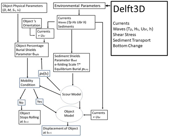
Figure 1.
Flow chart of the coupled Delft3D-object model to predict an objects’ mobility and burial.
The coupled system consists of two major components: Delft3D and object model. The object model has five parts: (a) a cylindrical object model with the burial percentage Shields parameter (θopb); (b) a sediment scour model with the sediment Shields parameter (θsed); (c) an object’s physical parameters such as diameter (D), relative density versus water density (So), mass (M), and rolling moment about its symmetric axis (Io); (d) environmental variables such as near seabed ocean currents, bottom wave orbital velocity (Ubr), water depth (h), wave peak period (TP), significant wave height (HS), and sediment characteristics; (e) the model output such as the burial percentage pB, and the object’s displacement.
The Target Reverberation Experiment 2013 (TREX13) in Panama City, Florida from 21 April to 13 May 2013 produced a unique data set containing environmental measurements such as waves, currents, and sediment samples, as well as mobility and burial of munitions [13]. The TREX13 data were used to verify the coupled model. The remainder of the paper is outlined as follows. Section 2 depicts the study area. Section 3 describes the observational data from TREX13. Section 4, Section 5 and Section 6 present the Delft3D, the object mobility model, and the object scour model. Section 7 presents the prediction of an object’s mobility and burial by the coupled Delft3D-object model. Section 8 presents the conclusions. Detailed object modeling information is included in Appendix A, Appendix B, Appendix C, Appendix D.
2. Study Area
The study area is off the coast of Panama City near the San Andrew Bay and is indicated by the region enclosed by the red lines in Figure 2. The tides are diurnal with an amplitude of highest astronomical tide (HAT) of 8.914 m and a maximum tidal range of 0.4 m [17]. The wind has strong seasonal variation: primarily from the north in winter and fall, and mostly from the south in summer and spring. The hurricane season in the Gulf of Mexico is typically from June to November with the peak occurring in August and September. During the off-hurricane season, the surface winds were not strong during 20 April–13 May 2013, with the east-west component (Figure 3a) and the north-south component (Figure 3b) from the NOAA buoy PACF1 (nearest to the study area) [18] and the ERA5 reanalysis data with 0.25° resolution from the European Centre for Medium-Range Weather Forecasts (ECMWF) [19]. It is noted that on 5 May 2013, a cold front was over northern Texas and passed over Panama City between 5–6 May 2013, causing a storm event and stronger waves. However, in general, the study area during the off-hurricane season represented a low-energy regime [13].
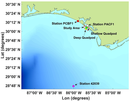
Figure 2.
Northern Gulf of Mexico of the coast of Panama City with locations of the shallow quadpod (30°04.81′ N, 85°40.41′ W), deep quadpod (30°03.02′ N, 85°41.34′ W), and the NOAA buoy stations PACF1, PCBF1, and 42039. The study area is enclosed by the red lines. The NOAA buoy station PACF1 is nearest to the study area.
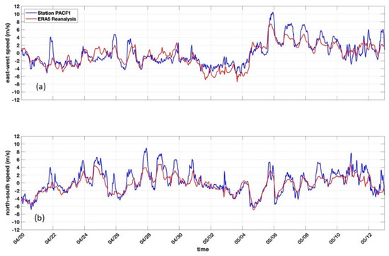
Figure 3.
Surface (a) east-west wind component and (b) north-south wind component for the study area from the NOAA PACF1 buoy (blue curves) [18] and the ERA5 reanalysis data with 0.25° resolution from the European Centre for Medium-Range Weather Forecasts (ECMWF) (red curves) [19].
3. TREX13
3.1. Surrogate Munitions
During TREX13, four types of surrogate and replica munitions were used to roughly represent the 155 mm HE M107, 81 mm mortar, 25 mm cartridge, and 20 mm cartridge and were designed and fabricated using crude drawings and specifications provided by existing Army Technical Manuals (e.g., TM 43-0001-27 and TM 43-0001-28) [13] (Figure 4). Table 1 shows the complete list of deployed and recovered munitions along with brief descriptions and their physical properties, such as bulk density and rolling moment, which are closely matched to their real counterparts.
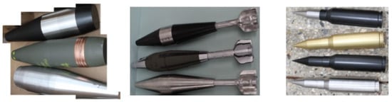
Figure 4.
Fabricated surrogates, purchased replicas, and fabricated replicas of (left) 155 mm HE M107, (middle) 81 mm mortars, and (right) 25 mm and 20 mm cartridges (from [13]).

Table 1.
List of surrogate and replica munitions used during TREX13. A total of 26 objects were deployed and 18 objects were recovered (from [13]). The surrogate munitions were fabricated to have rolling moments within 10% of the estimated rolling moment of the real counterpart.
3.2. Field Experiment
A field experiment was conducted to simultaneously collect both environmental (currents, waves, and sediment samples) data and the locations of surrogate/replica munitions on the seafloor from, 21 April 2013 to 13 May 2013, at two sites [13]. Instruments were mounted on a pair of large, rugged frames (herein referred to as “quadpods”) that were deployed at two different water depths (herein referred to as “deep” and “shallow”). The quadpods were deployed in the northern Gulf of Mexico offshore of Panama City Beach, FL, USA (Figure 5a). The deep quadpod was deployed at 30°03.02330 N, 85°41.33630 W, in about 20 m water depth, while the shallow quadpod was deployed at 30° 04.80994 N, 85° 40.41064 W, in about 7.5 m water depth. A sector scanning sonar was mounted on one of the legs of each of the quadpods, scanning a 110° swath every 12 min.
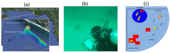
Figure 5.
(a) Locations of deep and shallow quadpods; (b) photo of divers laying the object field during the shallow quadpod deployment; (c) layout of objects laid by divers under the shallow quadpod (from [13]).
The data captured by TREX13 were during the time when hurricanes are “least” expected to occur. Therefore, the environmental conditions during hurricanes were ignored. This implies the hypothesis that the munitions’ mobility is not influenced by hurricane-generated waves and currents. This is because in shallow-water depths of 10–20 m, extreme significant wave heights resulting from hurricanes cause large near-bed-orbital velocities, leading to rapid scouring and burial and in turn stopping the munitions’ mobility.
The divers’ performance confirmed this hypothesis. Divers laid four surrogate munitions and nine replica munitions on the seafloor near each of the shallow and deep quadpods, within the view field of the sector scanning sonar, on 21 April 2013 (Figure 5b). The location and orientation of surrogate and replica munitions were detected by the sector scanning sonar and a maintenance diver with a video camera. Only objects laid by divers under the shallow quadpod were photographed (Figure 5c). The field of view of the sector scanning sonar is roughly represented by the light blue. The locations of the surrogates are denoted by a dark blue circle in the upper left. The other replicas were grouped according to relative bulk density. In this case, the red boxes denote the objects that were not recovered from the shallow quadpod site. Thus, the initial surrogate munitions’ location and orientation provided from TREX13 are only for the shallow quadpod. Immediately after the storm event on 5–6 May 2013, a maintenance dive was performed in the morning of 8 May 2013 and found that the surrogates and replicas may have been buried in place as opposed to being transported away by the waves and currents. Excavating by hand, divers were able to recover a total of eight munitions buried just below the surface, very near to the known initial locations at the shallow quadpod. The observational period for the munitions’ location and burial was 21 April–7 May 2013.
3.3. Data
As described in [13], the combined observations of munitions mobility and the driving environmental conditions were observed. Waves and currents were obtained using both acoustic surface tracking (Nortek AWAC) and a pressure time series. Two sediment cores were collected at the shallow quadpod location during deployment (core # D1) and retrieval (core # R1). It was found that both cores contained nearly 100% sand (Table 2). Therefore, the Shields parameter could be used for identifying the mobility of sediments. Grain size distributions were obtained with standard sieve techniques and results for porosity, bulk density, and void ratio were obtained by measuring the weight loss or water weight. The median grain diameter (d50) is around 0.23 mm, and the sediment density (ρs) is about 2.69 × 10³ kg m−3. These two parameters are most significant to influencing sediment mobility and are needed for the object scour burial model (see Section 6).
Table 2.
Sediment properties from diver push cores taken during the deployment (D1) and the retrieval (R1) of the instrumentation at the shallow quadpod location (from [13]).
4. Delft3D
4.1. Model Description
The open-source Delft3D version 4.04.01 was implemented in the TREX13 area to predict currents and waves. Under the wind and tidal forcing, the flow module [10] predicts the water level, currents, feeds the current data into the wave and morphology modules as input, computes the sediment transport, and updates the bathymetry. The wave module [11] is used to predict the wave generation, propagation, dissipation, and non-linear wave–wave interactions in the nearshore environment with inputs such as water level, bathymetry, wind, and currents from the flow module. The wave module uses Simulating Waves Nearshore (SWAN), which is a third-generation model derived from the Eulerian wave action balance equation [12]. Since we are only interested in the wave parameters such as the peak period (TP), significant wave height (HS), and bottom wave orbital velocity (Ubr), with a temporal resolution of 1 h for the object model, the coupling time between the flow and wave modules was also set to 1 h. The morphology module works in an integrated way with the wave and flow modules in a cycle. This system is a process-based model that considers the impact of waves, currents, and sediment transport on morphological changes. In this study, the sediment module was not activated.
4.2. Model Grids and Time Steps
Two grids with different grid cell sizes were nested (Figure 6) to create a region with finer resolution. These rectangular grids compose the flow domain. The flow outer grid (coarser resolution) is composed of 137 × 75 grid points with spacing of 50 m in both longshore and cross-shore directions. The flow inner grid (finer resolution) has 20 m resolution and was divided into 139 × 124 grid points, equally spaced. The sediment transport and morphological evolution were computed only in the flow inner grid. The wave domain (Figure 6) was defined in order to avoid the boundary effect and allow the use of deep quadpod data to set up the wave boundary conditions. The wave grid is composed of 273 × 111 grid points with 50 m resolution. The bathymetric data (Figure 6) were from the Northern Gulf Coast Digital Elevation Model from the National Oceanic and Atmospheric Administration/National Geophysical Data Center (NOAA/NGDC) [20]. The resolution of this data set varies between 1/3 arc-second and 1 arc-second (around 10 and 30 m). The time step is set as 0.2 s for the coarse domain (grid size 50 m) and 0.1 s for the finer domain (grid size 20 m). The small time-steps (0.2 s, 0.1 s) are needed in order to satisfy the Courant–Friedrichs–Lewy (CFL) condition of computational stability for the Delft3D flow module.
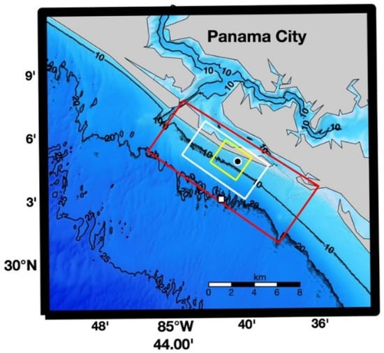
Figure 6.
Study area with bathymetry, depth contours (10 m, 20 m, and 25 m), and computational grids for wave module (red), flow module with coarse resolution (white), and flow module with fine resolution (yellow). The black dot represents the shallow quadpod location, and the white square denotes the deep quadpod location (from [17]).
4.3. Wind and Tidal Forcing
The wind input files were set up using ERA5 reanalysis data from the European Centre for Medium-Range Weather Forecasts (ECMWF), with 0.25° resolution [19] for the flow and wave modules. The Global Inverse Tide Model TPXO 8.0 with 1/45-degree resolution was used to create the boundary conditions for the flow module. For the alongshore boundary, the water level with astronomic forcing was imposed. The water level gradient (a so-called Neumann boundary condition) was chosen with a constant zero water level slope in the longshore direction for both across-shore open boundaries. It allows for flow to leave and enter the lateral boundaries with no spurious circulation.
4.4. Initial and Boundary Conditions
As an initial condition, the water level and current velocity were set to zero. Additionally, the sediment transport boundary conditions were set by specifying the inflow concentration as zero kg/m3. The initial condition for the sand sediment was set as a uniform zero concentration, and the initial bed of sediment was set to 5 m. Wave boundary conditions were set based on the measurements from the deep quadpod location using the significant wave height, wave period, wave directions, and directional spreading. These parameters were applied uniformly on the three open boundaries. A spin-up interval of 720 min was established to prevent any influence from a possible initial hydrodynamic instability on the bottom change calculation, which starts only after the spin-up interval. The sediment type was set as sand with a sediment-specific density of 2650 kg/m3.
The calibration was conducted to adjust the parameters to the best agreement between the modeled and observed water level, waves, and currents. For water level, calibration was done through minimizing the difference in amplitude and phase between predicted and measured tides. For waves, the calibration was to determine the optimal JONSWAP bottom friction coefficient and wave height to water depth ratio. For currents, the calibration was to identify the best Chézy bottom roughness as well as horizontal eddy viscosity and diffusivity. The calibration period was set up as 21–27 April 2013, which corresponds to 27% of the entire period of observations (21 April–13 May). During this process, parameters were adjusted separately. While one was fine-tuned, the others remained constant. The calibrated JONSWAP bottom friction coefficient was 0.067 m2/s3 and the wave height to water depth ratio was 0.7, for the wave module. The Chézy bottom roughness was 65 m1/2/s, horizontal eddy viscosity was 0.5 m2/s, and horizontal diffusivity was 10 m2/s, for the flow module.
4.5. Model Output
The Delft3D output data with 1-h resolution are used as input for the object model. The output from the flow module includes the water depth (h) and the current velocity, Uc = ive + jvn, with (i, j) the unit vectors in longitudinal and latitudinal directions, and Uc = (ve2 + vn2)1/2 as the current speed. The output from the wave module includes the wave peak-period (TP), significant wave height (HS), wave direction, and bottom wave orbital velocity (Ubr). The bottom water velocity vector of combined current and waves is represented by Vw with |Vw| = Uc + Ubr and the orientation ψ = tan−1(vn/ve). Figure 7 shows the time series of the environmental parameters [ve, vn, h, TP, HS, Ubr] predicted by the Delft3D (red curve) and observed by the AWAC (black curve). The AWAC only provides the observed data for [ve, vn, h, TP, HS], but not the bottom orbital velocity Ubr, which was calculated using a well-established linear wave model with a Matlab function [21] using the observed water depth (h), significant wave height (HS), and peak period (Tp) (see Appendix D in [21]).
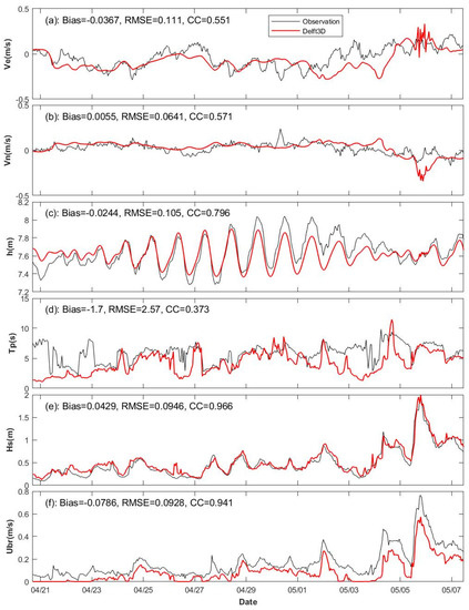
Figure 7.
Comparison of Delft3D predictions (red) and observations during TREX13 (black) at the shallow quadpod from 21 April to 7 May 2013: (a) near bed (~0.15 m) longitudinal current ve (m/s); (b) near bed (~0.15 m) latitudinal current vn (m/s); (c) water depth h (m); (d) peak period TP (s); (e) significant wave height HS (m); (f) computed bottom wave orbital velocity Ubr (m/s).
Since the munitions were found totally buried, without mobility, on the morning of 8 May 2013 by the divers in TREX13, and TREX13 provides the munitions’ mobility information from 21 April to 7 May 2013, the integration period for the coupled Delft3D-object model was set as 21 April–7 May 2013. The root-mean-square error (RMSE) between the Delft3D output and the TREX13 observations is 0.105 m for the water level, 0.111 m/s for the east-west current speed, 0.0641 m/s for the north-south current speed, 0.0946 m for the significant wave height, and 0.0928 m/s for the bottom wave orbital velocity. The bias between the Delft3D output and the TREX13 observations is −0.0244 m for the water level, −0.0367 m/s for the east-west current speed, 0.0055 m/s for the north-south current speed, 0.0429 m for the significant wave height, and −0.0786 m/s for the bottom wave orbital velocity. The correlation coefficient between the Delft3D output and the TREX13 observations is as high as 0.966 for the significant wave height, 0.941 for the bottom wave orbital velocity, reasonably high as 0.796 for the water depth, 0.571 for the north-south current speed, 0.551 for the east-west current speed, and the lowest at 0.373 for the peak wave period. The Delft3D modeling performed reasonably well according to the criteria presented in [22].
5. Object Mobility Model
Consider a cylindrical object with length L and diameter D buried in the seabed with the burial depth B (B < D/2). Let the water velocity (consisting of current and waves) near the seabed (Vw) be in the direction towards the cylinder with an angle, ϕ, perpendicular to the main axis of the cylinder and be decomposed into Vw = (U, V), with U being the perpendicular component and V the parallel component (Figure 8) to the main axis of the cylinder. As the object rolls with angular velocity on the seabed with the object’s burial, let the axis of rotation inside the sediment be at depth b (b < B) (see Appendix A).
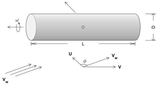
Figure 8.
Roll of a cylindrical object on the seafloor with large aspect ratio forced by the combination of ocean currents and bottom wave orbital velocity. Here, (π/2 − ϕ) is the angle between Vw and the main axis of the cylinder.
As an object rolls around point b (see Figure A1 in Appendix A) with an angular velocity , the translation velocity of the object is given by:
The corresponding moment of momentum equation of the rolling object is given by [see Equation (A17) in Appendix B]:
where ; Io is the rolling moment of the munition about the symmetric axis of the munition (see Figure A2); TF is the forward torque caused by the drag force (Fd) and lift force (Fl) (see Appendix C); pB = B/D, is the percentage burial, and θopb is the object mobility parameter for percentage burial (see Appendix B); (ρo, ρw) are the densities of the object and water; Π is the volume of the munition.
Let the relative horizontal velocity of the rolling object be defined by:
Substitution of (1) into (2) and use of (3) leads to a special Riccati equation,
where
The special Riccati Equation (4) has an analytical solution from integration from tk to tk + 1 (k = 0, 1, 2,…, K−1) [23]
with αk and βk as known constants during the integration. Substitution of (6) into (3) leads to the dimensional horizontal velocity of the rolling object, uo(t) = U(t), which should be used for each time interval Δt. The solution (6) depends on (αk, βk) which involve three types of parameters: (a) time-independent physical parameters of the object for So, Π, L, and D; (b) time-dependent water velocity, U(tk), from the Delft3D model output; (c) time-dependent relative depth of sediment rolling axis [pb(tk)] and burial percentage [pB(tk)] determined using a scour burial model. Let l be the displacement of the object,
Integration of l with respect to time t leads to the munition’s displacement.
6. Object Scour Model
Existing studies on scour burial were all concentrated on motionless objects. The ratio between the fluid force (bottom shear stress) and the weight of the sediment particles, i.e., the sediment Shields parameter (θsed),
is crucial for scour burial of motionless objects and in turn for prediction of the percentage burial parameter pB(t) = B/D [15,16]. Here, f is the wave friction factor [24], ρs the sediment grain density, and d50 the medium sand grain size. Using the wave data (TP, Ubr) from Figure 6 e.g., and sediment parameters (ρs = 2.69 × 10³ kg/m3, d50 = 0.23 × 10⁻³ m) from TREX13 [9,13], the sediment Shields parameters (θsed) were calculated from 21 April to 7 May 2013. The results were less than 0.1 every time, except when atmospheric cold fronts passed by on 5–6 May 2013. The maximum value of θsed reached 0.33 (Figure 9).
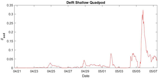
Figure 9.
Time series of sediment Shields parameter (θsed) at the shallow quadpod computed from the Delft3D model output.
As pointed out in [24], the equilibrium percentage burial pB,eq for motionless cylinders induced by scouring tends to increase as θsed increases. An empirical formula has been established,
with different choices of the coefficients (a1, a2, a3) determined experimentally for cylinders subject to steady currents: a1 = 11, a2 = 0.5, a3 = 1.73 [25], a1 = 0.7, a2 = a3 = 0 [26], a1 = 2, a2 = 0.8, and a3 = 0 [27]. For cylinders under waves (depending on wave period): a1 = 1.6, a2 = 0.85, and a3 = 0 for Tp longer than 4 s [28]. For motionless cylinders, before scour burial reaches equilibrium, the percentage burial follows an exponential relationship [25],
where the e-folding time scale T* is given by
With the bottom wave orbital velocity (Ubr), sediment density(ρs), medium grain size (d50), and in turn the sediment Shields parameter (θsed), the equilibrium object percentage burial (pB,eq) is calculated using (9) with coefficients a1 = 1.6, a2 = 0.85, and a3 = 0. The sediment supporting depth b (or pb) is calculated from burial depth B (or pB) using (10), i.e.,
It is noted that the predicted burial percentage (pB) computed from (10) represents the depth that an object on the surface would bury to at that moment, but an object deployed at the beginning of the time sequence would always remain buried at the deepest burial it has reached so far. The burial depth of the base of the object below the ambient seabed is equivalent to the greatest depth that the scour pit has reached up to that point in time [29]. In other words, scouring only acts to bury an object deeper. It can never be unburied (re-exposure), as the time series is suggested by (10). Similar to [29], a simple parameterization was proposed [9] to represent the re-exposure process starting from k (= 1, 2, …): (a) doing nothing if , (b) computing the weighted average
with w being the weight coefficient. In this study, we take w = 0.80. The object mobility and burial model consists of Equations (6)–(13).
7. Prediction of Object’s Mobility and Burial
The munitions’ mobility and burial were predicted using object mobility and burial models, with the environmental variables predicted by the Delft3D (Figure 1) as the forcing term. The model was integrated for each surrogate (or replica) munition deployed in the shallow quadpod with its initial location and orientation (Figure 5c) at 12:40 (14:00) local time on 20 April 2013. The angle between Vw (data represented by the red curves in panels a, b in Figure 7) and the direction perpendicular to cylinder’s main axis is determined. The velocity vector of combined current and waves (Vw) is then transformed into Vw = (U, V) with U being the perpendicular component, and V the paralleling component. The component U is used in the model. The object’s physical parameters, such as the diameter (D), volume, mass (M), and density (ρo), are obtained from Table 1.
The environmental data, such as the water depth (h), wave peak period (TP), significant wave height (HS), bottom wave orbital velocity (Ubr) (represented by the red curves in Figure 7), and sediment data (100% sand, d50 = 0.23 mm, ρs = 2.69 × 10³ kg m−3) are used by the sediment scour model (i.e., Equations (8)–(13)) to get the burial percentage pB(tk), and in turn the relative rolling center depth pb(tk). With the object’s physical parameters (D, ρo, M), the calculated pb(tk), model-predicted bottom current velocity component perpendicular to the object’s main axis U(tk), and the coefficients [α(tk), β(tk)] for the object mobility model (i.e., Equation (5)), the object’s displacement at the next time step l(tk + 1) can be predicted using (7).
Based on the known initial locations of the objects at the shallow quadpod (Figure 5c), the model predicts the objects’ burial percentage (pB(tk)) shown in Figure 10, the objects’ mobility parameter for percentage burial (θopb(tk)) shown in Figure 11, and the objects’ displacement (l(tk)) shown in Figure 12. The burial percentages pB for all the objects were less than 0.5, except during the storm event at 12:00 on 5 May to 00:00 on 6 May 2013 local time (Figure 10). The red color in Figure 11 shows that the objects’ rolling condition [θopb > 1] is satisfied.
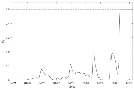
Figure 10.
Model predicted burial percentage pB(t) with re-exposure parameterization (13) for each object at the shallow quadpod from 20 April to 7 May 2013. The predicted burial percentage pB(t) is less than 0.5 for all the munitions during the whole time period, except during the storm event from 12:00 5 May to 00:00 6 May 2013. The burial percentage pB(t) is the same for each object, since it only depends on the sediment characteristics [see Equations (9)–(11)].
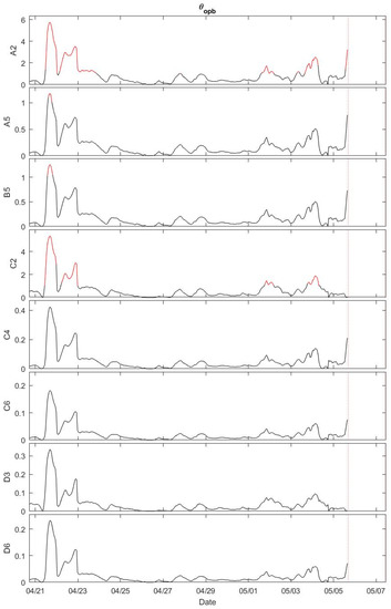
Figure 11.
Model predicted objects’ mobility parameters for percentage burial (θopb) at the shallow quadpod from 20 April to 7 May 2013. The red color shows that the condition for rolling an object [θopb > 1] is satisfied. The parameters θopb is not computed between 12:00 5 May to 00:00 6 May 2013, since the predicted burial percentage pB(t) is larger than 0.5. Among the eight objects, only A2 and C2 have evident time periods when the condition for rolling an object [θopb > 1] is satisfied.
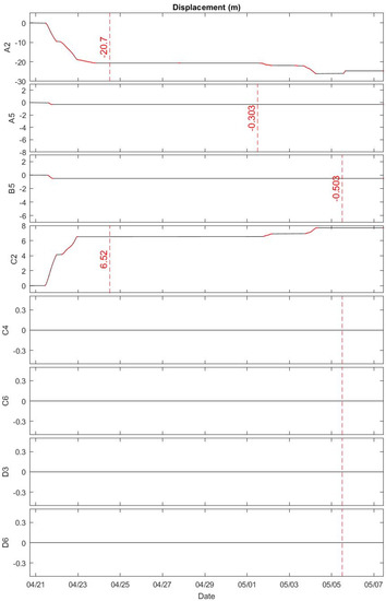
Figure 12.
Model predicted displacement l(t) for each object at the shallow quadpod from 20 April to 7 May 2013. Among the eight objects, only A2 and C2 were immediately mobile and displaced 20.7 m (A2) and 6.52 m (C2) on 12:00 24 April 2013 (dashed line). Other munitions A5, B5, C4, C6, D3, D6 were completely motionless. According to the TREX13 report [13], the objects A2 and C2 were immediately mobile and transported out of the field of view because they were last seen on 23 April 2013. After 23 April 2013, their locations have never been observed.
The surrogate and replica munitions’ mobility and burial were observed by divers and sector scanning sonar images during the field experiment depicted in Section 2 and in [13]. A total of eight munitions at the shallow quadpod location were recovered by divers during the maintenance dive performed on 8 May 2013 (Figure 5b). Note that the munitions excavated by the divers at the shallow quadpod location on 8 May 2013 were immediately redeployed for the duration of the experiment. An overview of the observed munitions’ mobility throughout the whole TREX13 experiment (20 April to 7 May 2013) is shown in Figure 13a and during the storm event from 13:00–20:00 on 5 May 2013 in Figure 13b. The objects A2 and C2 were immediately mobile and transported out of the field of view; they were last seen on 23 April 2013 (very crude observational information). However, the other objects were nearly immobile (Figure 13a). The predicted large displacements of 20.7 m for A2 from 12:00 21 April to 12:00 24 April 2013 and 6.52 m for C2 from 12:00 21 April to 00:00 23 April 2013 (Figure 12) qualitatively agree with the crude observational information about A2 and C2.
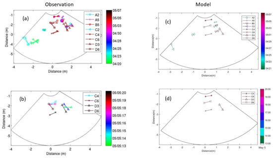
Figure 13.
Positions for all visible objects at the shallow quadpod location up to the maintenance dive performed on 8 May: (a) observation for 20 April–7 May 2013; (b) observation for 13:00–20:00 on 5 May 2013; (c) model prediction for 20 April–7 May 2013; (d) model prediction for 13:00–20:00 on 5 May 2013. Note that Figure 13a,b were copied from [13]. The color bars denote the last time when each object was visible with dates for (a,c) and hour on 5 May for (b,d).
Furthermore, overview of the modeled objects’ mobility throughout the whole TREX13 experiment (20 April to 7 May 2013) is shown in Figure 13c and during the storm event from 13:00–20:00 on 5 May 2013 in Figure 13d. Similarity between observation (Figure 13a,b) and the model prediction (Figure 13c,d) shows model capability. However, model–data discrepancy exists. For example, the yaw of munitions D3 and D6 was observed (Figure 13a,b), but not predicted (Figure 13c,d). The munition D3 (rightmost triangles in Figure 13a,b) moved, but the model predicted a value of l = 0 m by predicting that D3 would never move (Figure 10 and Figure 13c,d). The model limitation is due to these four assumptions: (a) cylinder with a large aspect ratio (L D); (b) no yaw and pitch; (c) a percentage burial depth of less than 0.5; (d) a flat seabed. Even if the bottom profile is flat when the object is deployed, the sand tends to accumulate in front of the object and erodes on the opposite side, thus creating a wavy bed that affects the dynamics of the object. The model will lose capability in the real world if the shape of munitions is evidently different from the cylinder with and the effect of a wavy seabed is large on the dynamics of the object.
8. Conclusions
- (1)
- A coupled Delft3D-object model was recently developed to predict underwater cylindrical objects’ mobility and burial in a sandy bed. The roll of the object is the major dynamic of this model, with a new concept of its rolling center in the sediment. The object’s displacement caused by rolling satisfies the Riccati equation with an analytical solution. Along with the dynamical model, the empirical scour model with re-exposure parameterization is used as part of the prediction system.
- (2)
- Data collected at the shallow quadpod during TREX13 (21 April to 23 May 2013) off the coast of Panama City, Florida were used as model verification. The environmental data, such as bottom currents, water depth (h), peak period (Tp), and significant wave height (HS), are used to verify the Delft3D model. The objects’ positions tracked by sector scanning sonar images and maintenance divers are used to verify the object’s mobility and burial model.
- (3)
- The model predicted object positions agree qualitatively well with the observed surrogates (or replicas) data. Observation shows that objects A2 and C2 were immediately mobile and transported out of the field of view, because they were last seen on 23 April 2013. The other objects were nearly immobile. The objects with large mobility are A2 (displaced 20.7 m from 12:00 21 April to 12:00 24 April 2013) and C2 (displaced 6.52 m for C2 from 12:00 21 April to 00:00 23 April 2013). A2 is a 20 mm cartridge with a mass of 0.11 kg and a density of 1429 kg m−3. C2 is an 81 mm mortar with a mass of 1.45 kg and a density of 1.199 kg m−3 (see Table 1). The other objects, with almost no mobility, are A5 (density of 2597 kg m−3), B5 (density of 2356 kg m−3), C4 (density of 3109 kg m−3), C6 (density of 7194 kg m−3), D3 (density of 2721 kg m−3), and D6 (density of 4444 kg m−3). The larger the object’s density, the smaller the object’s mobility parameter for percentage burial (see Equation (A14)). However, it is noted that the observational object data are quite crude and not sufficient to accurately verify the model prediction on an object’s mobility and burial.
- (4)
- Although the coupled Delft3D-object model has the capability to predict an object’s mobility, the model has its own weakness specifically regarding cylindrical objects. It only considers the roll of the cylinder around its major axis. The object model ignores pitch and yaw. Besides, the seabed is assumed to be flat. It is necessary to extend the object modeling to more realistic seabed environments, object shapes, and more complete motions for operational use.
Author Contributions
Methodology, P.C.C.; software, V.S.P. and C.F.; validation, P.C.C., V.S.P. and C.F.; formal analysis, P.C.C.; investigation, P.C.C.; resources, P.C.C.; experimental data collection, J.C.; writing—original draft preparation, P.C.C.; writing—review and editing, P.C.C.; visualization, V.S.P. and C.F.; supervision, P.C.C.; project administration, P.C.C.; funding acquisition, P.C.C. All authors have read and agreed to the published version of the manuscript.
Funding
This research was funded by the Department of Defense Strategic Environmental Research and Development Program (SERDP), grant numbers N6227C20WA00DCE and N6227C21WA00AWC.
Acknowledgments
The authors would like to thank the Munitions Response Program of the Strategic Environmental Research and Development Program for financial support under projects MR19-1073, MR19-1317, and MR-2320.
Conflicts of Interest
The authors declare no conflict of interest.
Appendix A
Location of Object’s Rotation Axis in Sediment.
Roll of an object on the sandy floor needs a supporting point in sediment. The compressive normal stress of sediment on the object is represented by
where n is the unit vector normal to the cylinder surface, and is the compressive coefficient. Let n be decomposed into
where (eh, ev) are horizontal and vertical unit vectors (see Figure A1). The sediment compressive normal stress FS is decomposed as,
With b as the axis of rotation, the sediment above (below) the depth b generates torque to resist (enhance) the rolling with the total torque from the sediment,
where r is the position vector at any point on the circle and rb is the position vector at point b with point E as the origin,

Figure A1.
The location of the axis of rotation of the cylinder in the sediment, b, is determined by the assumption of zero-sum torque to the roll.
Figure A1.
The location of the axis of rotation of the cylinder in the sediment, b, is determined by the assumption of zero-sum torque to the roll.

The depths B and b are represented by
If we assume that at the depth b the total torque from the sediment is zero (i.e., zero-sum sediment torque for rolling),
Substitution of (A3)–(A5) into (A7) gives
The ratio λ = b/B can be obtained from (A6) and (A8),
The ratio, λ, varies with the burial percentage pB = B/D mildly from near 0.4445 for pB = 0 and 0.4630. Here, we take λ = 0.453 in this study.
Appendix B
Dynamics of Rolling Object.
The drag force (Fd) and lift force (Fl) (see Appendix C) roll the object forward with the torque TF (Figure A2),
The buoyancy force and added mass roll the object backward with the torque, TB = Tw + Ta,

Figure A2.
Forces and torques due to drag, lift, buoyancy, and added mass on a partially buried cylinder by combination of ocean currents and bottom wave orbital velocity (U) perpendicular to the major axis of the cylinder.
Figure A2.
Forces and torques due to drag, lift, buoyancy, and added mass on a partially buried cylinder by combination of ocean currents and bottom wave orbital velocity (U) perpendicular to the major axis of the cylinder.

When TF > TB the object accelerates if it is in motion or starts to move if it is at rest (uo = 0, duo/dt = 0). When TF < TB the object decelerates if it is in motion or keeps motionless if it is at rest. When TF = TB the object keeps velocity constant if it is in motion or keeps motionless if it is at rest. Thus, the threshold for the munition’s mobility becomes
The acceleration-deceleration ratio is defined by
where
Here, θopb is the object’s mobility parameter for percentage burial pb [14] and So is the relative density of the object. For motionless munition (uo = 0), the condition for the object to move is obtained through substituting (A13) into (A12)
The corresponding moment of momentum equation of the rolling object is given by
Substitution of (TF, TB) in (A10) (A11) into (16) leads to
with
where Io is the rolling moment about the symmetric axis of the munition; IA is the rolling moment of munition about the point b (see Figure A2) using the parallel axis theorem; Π is the volume of the munition.
Appendix C
Drag, Lift, Buoyancy Forces, and Added Mass.
The drag force (Fd), lift force (Fl), buoyancy force (Fw), and added mass (Fa) exerted on the object for rolling by the perpendicular component, U, are given by
where g = 9.81 m/s2 is the gravitational acceleration; ρw = 1025 kg/m3 is the density of seawater; ρo is the density of the cylindrical object; (Cd, Cl) are the drag and lift coefficients across-cylinder’s main axis, with vortex shedding caused by the oscillating flow (U) due to waves. If time averaged U within a certain time period being used, the mean coefficients for drag and lift (Cd, Cl), depending solely on the Reynolds number and aspect ratio (see Appendix D), can be used. Since the wave component (i.e., the bottom wave orbital velocity) in Vw for the object model is computed from a linear wave model with the temporal resolution of 30 min, the mean coefficients for drag and lift are used. The vortex shedding from objects is neglected. Besides, when the lift coefficient is less certain, we assume
where γ is the ratio of lift coefficient versus drag coefficient with γ being taken as value of 0.2.
Appendix D
Drag Coefficient.
For cylindrical objects, the drag force is decomposed into along and cross axis components. The drag coefficient across-cylinder’s main axis Cd depends on the Reynolds number,
where = 0.8 × 10⁻⁶ m2/s, is the sea water kinematic viscosity; U is the horizontal water velocity perpendicular to the cylinder’s main axis; and D is the cylinder’s diameter (see Figure 6). For an empirical formula used to calculate Cd [30].
where η = L/D, is the cylinder’s aspect ratio.
References
- SERDP. Munitions in the Underwater Environment: State of the Science and Knowledge Gaps—White Paper. 2010. Available online: https://www.serdp-estcp.org/Featured-Initiatives/Munitions-Response-Initiatives/Munitions-in-the-Underwater-Environment (accessed on 13 February 2021).
- Bennett, R.H. Mine Burial Prediction Workshop Report and Recommendations; Prepared for ONR; Technical Report Number SI-0000-02; Office of Naval Research: Arlinton, VA, USA, 2000; pp. 1–21.
- Chu, P.C. Mine impact burial prediction from one to three dimensions. Appl. Mech. Rev. 2009, 62, 25. [Google Scholar] [CrossRef]
- Chu, P.C.; Fan, C.W.; Evans, A.D.; Gilles, A.F. Triple coordinate transforms for prediction of falling cylinder through the water column. J. Appl. Mech. 2004, 71, 292–298. [Google Scholar] [CrossRef][Green Version]
- Chu, P.C.; Gilles, A.F.; Fan, C.W. Experiment of falling cylinder through the water column. Exp. Therm. Fluid Sci. 2005, 29, 555–568. [Google Scholar] [CrossRef]
- Chu, P.C.; Fan, C.W. Mine impact burial model (IMPACT35) verification and improvement using sediment bearing factor method. IEEE J. Ocean. Eng. 2007, 32, 34–48. [Google Scholar] [CrossRef]
- Chu, P.C.; Fan, C.W. Pseudo-cylinder parameterization for mine impact burial prediction. J. Fluids Eng. 2005, 127, 1515–1520. [Google Scholar] [CrossRef][Green Version]
- Chu, P.C.; Fan, C.W. Prediction of falling cylinder through air-water-sediment columns. J. Appl. Mech. 2006, 73, 300–314. [Google Scholar] [CrossRef][Green Version]
- Chu, P.C.; Fan, C.W.; Calantoni, J.; Sheremet, A. Prediction of mobility and burial of object on sandy seafloor. IEEE J. Ocean. Eng. in press.
- Deltares. Delft3D-Flow—Simulation of Multi-Dimensional Hydrodynamic Flows and Transport Phenomena, Including Sediments; User Manual. 2019. Available online: https://content.oss.deltares.nl/delft3d/manuals/Delft3D-FLOW_User_Manual.pdf (accessed on 21 September 2020).
- Deltares. Delft3D-Wave—Simulation of Short-Crested Waves with SWAN; User Manual. 2019. Available online: https://content.oss.deltares.nl/delft3d/manuals/Delft3D-WAVE_User_Manual (accessed on 21 September 2020).
- Booij, N.; Ris, R.C.; Holthuijsen, L.H. A third-generation wave model for coastal regions: 1. Model description and validation. J. Geophys. Res. 1999, 104, 7649–7666. [Google Scholar] [CrossRef]
- Calantoni, J.; Staples, T.; Sheremet, A. Long Time Series Measurements of Munitions Mobility in the Wave-Current Boundary Layer; Interim Report; Project MR-2320; US Strategic Environmental Research and Development Program SERDP: Alexandria, VA, USA, 2014; p. 48. [Google Scholar]
- Traykovski, P.; Austin, T. Continuous Monitoring of Mobility, Burial, and Re-Exposure of Underwater Munitions in Energetic Near-Shore Environments; Final Report; Project MR-2319; US Strategic Environmental Research and Development Program SERDP: Alexandria, VA, USA, 2017; p. 44. [Google Scholar]
- Friedrichs, C.T.; Rennie, S.E.; Brandt, A. Self-burial of objects on sandy beds by scour: A synthesis of observations. In Scour and Erosion; Harris, J.M., Whitehouse, R.J.S., Eds.; CRC Press: Boca Raton, FL, USA, 2016; pp. 179–189. ISBN 978-1-138-02979-8. [Google Scholar]
- Rennie, S.E.; Brandt, A.; Friedrichs, C.T. Initiation of motion and scour burial of objects underwater. Ocean Eng. 2017, 131, 282–294. [Google Scholar] [CrossRef]
- Bunya, S.; Dietrich, J.C.; Westerink, J.; Ebersole, B.A.; Smith, J.M.; Atkinson, J.H.; Jensen, R.; Resio, D.T.; Luettich, R.A.; Dawson, C.; et al. A high-resolution coupled riverine flow, tide, wind, wind wave, and storm surge model for Southern Louisiana and Mississippi, part 1; model development and validation. Mon. Weather Rev. 2010, 138, 345–377. [Google Scholar] [CrossRef]
- NOAA National Data Buoy Center. Surface Wind Vector Data at the Station PACF1 8729108—Panama City, FL. Available online: https://www.ndbc.noaa.gov/station_page.php?station=pacf1 (accessed on 25 January 2021).
- ECMWF. ERA5 Reanalysis (0.25 Degree Latitude-Longitude Grid). Research Data Archive at the National Center for Atmospheric Research, Computational and Information Systems Laboratory, Boulder, CO. Available online: https://rda.ucar.edu/datasets/ds633.0 (accessed on 25 January 2021).
- NOAA/NGDC. Northern Gulf 1 Arc-Second MHW Coast Digital Elevation Model. Available online: https://catalog.data.gov/dataset/northern-gulf-coast-digital-elevation-model156ed (accessed on 17 December 2018).
- Wiberg, P.L.; Sherwood, C.R. Calculating wave-generated bottom orbital velocities from surface wave parameters. Compt. Geosci. 2008, 34, 1243–1262. [Google Scholar] [CrossRef]
- Van Rijn, L.C.; Walstra, D.; Grasmeijer, B.; Sutherland, J.; Pan, S.; Sierra, J. The predictability of cross-shore bed evolution of sandy beaches at the time scale of storms and seasons using process-based Profile models. Coast. Eng. 2003, 47, 295–327. [Google Scholar] [CrossRef]
- Kamke, E. Differentialgleichungen: Losungsmethoden und Losungen, I, Gewohnliche Differentialgleichungen; B. G. Teubner: Leipzig, Germany, 1977. [Google Scholar]
- Nielsen, P. Coastal Bottom Boundary Layers and Sediment Transport; Advanced Series on Ocean Engineering 4; World Scientific: Singapore, 1992; p. 324. [Google Scholar]
- Whitehouse, R. Scour at Marine Structures: A Manual for Practical Applications; Thomas Telford Publications: London, UK, 1998; p. 198. [Google Scholar]
- Sumer, B.M.; Truelsen, C.; Sichmann, T.; Fredsøe, J. Onset of scour below pipelines and self-burial. Coast. Eng. 2001, 42, 313–335. [Google Scholar] [CrossRef]
- Demir, S.T.; García, M.H. Experimental studies on burial of finite length cylinders under oscillatory flow. J. Waterw. Port Coast. Ocean Eng. 2007, 133, 117–124. [Google Scholar] [CrossRef]
- Cataño-Lopera, Y.A.; Demir, S.T.; García, M.H. Self-burial of short cylinders under oscillatory flows and combined waves plus current. IEEE J. Ocean. Eng. 2007, 32, 191–203. [Google Scholar] [CrossRef]
- Trembanis, A.C.; Friedrichs, C.T.; Richardson, M.D.; Traykovski, P.; Howd, P.A.; Elmore, P.A.; Wever, T.F. Predicting seabed burial of cylinders by wave-induced scour: Application to the sandy inner shelf off Florida and Massachusetts. IEEE J. Ocean. Eng. 2007, 32, 167–183. [Google Scholar] [CrossRef]
- Rouse, H. Fluid Mechanics for Hydraulic Engineers, 1st ed.; Mcgraw-Hill Book Company Inc.: New York, NY, USA, 1938; p. 422. [Google Scholar]


Publisher’s Note: MDPI stays neutral with regard to jurisdictional claims in published maps and institutional affiliations. |
© 2021 by the authors. Licensee MDPI, Basel, Switzerland. This article is an open access article distributed under the terms and conditions of the Creative Commons Attribution (CC BY) license (https://creativecommons.org/licenses/by/4.0/).