Nonlinear Wave Transformation in Coastal Zone: Free and Bound Waves

Abstract

The nonlinear transformation of waves in the coastal zone over the sloping bottom is considered on the base of field, laboratory, and numerical experiments by methods of spectral and wavelet analyses. The nonlinearity leads to substantial changes of wave shape during its propagation to the shore. Since these changes occur rapidly, the wave movement is non-periodical in space, and the application of linear theory concepts of wavenumber or wavelength results in some paradoxical phenomena. When analyzing the spatial evolution of waves in the frequency domain, the effect of periodic energy exchange and changes in the phase shift between the first and second wave harmonics are observed. When considering the wavenumber domain, the free and bound waves of both the first and second harmonics with constant in space amplitudes appear, and all spatial fluctuations of the wave parameters are caused by interference of these four harmonics. Practically important consequences such as the wave energy spatial fluctuations and of anomalous dispersion of the second harmonic are shown and discussed.

1. Introduction

Waves are the main source of energy in the coastal zone of the sea and therefore wave transformation is a factor determining many dynamic processes. In addition, waves affect shore structures, and knowledge about the change in their parameters as the waves approach the shore is necessary to design shore protection from wave impact. The wave parameters and regularities of their change are necessary for solving practical and theoretical problems for the development and recreational exploitation of any coastal zone.

The main feature of nonlinear wave transformation in the coastal zone over slopping bottom is the generation of high-frequency wave components. For the first time, the introduction of free and bound waves in the context of nonlinear wave interaction was done in [1] for the case of four wave interactions on deep water. It was shown that free waves corresponding to dispersion relation during nonlinear interactions can generate bound waves. For the dynamic processes on shallow and intermediate water depth, more important is the second harmonic that consists of free and bound modes. This fact is well-known in the coastal engineering community. However, detailed description of the influence on coexisting free and bound waves on the evolution of wave parameters in the coastal zone is missing due to absence of analytical solutions and the difficulties to measure the simultaneous time and spatial fluctuations of free surface elevations in physical experiments.

The second nonlinear wave harmonic is important because it is responsible for the shoreward wave component of sediment discharge q. in accordance with the popular sediment discharge formula, introduced by Bailard [2] and then simplified by Stive [3]

$$q\approx A{u}_1^2{u}_2\cos \left(\phi \right)+B{u}_1^3{u}_2 \cos \left(\phi \right)$$

(1)

where u₁ and u₂ are the amplitudes of first and second harmonics of near-bottom wave velocity which are linearly proportional to the corresponding wave harmonics and φ is the phase shift between them. If u₂ = 0 or φ = ±π/2, then q will be equal to 0. In this case beach erosion will occur because there will be no wave component of sediment transport to the shore and the undertow directed to the sea will prevail.

It was shown that the spatially periodic exchange of energy between the first and second harmonics contributes to the formation and movement of underwater sand bars [4,5]. In addition, the periodic exchange of energy between harmonics leads to the arising and disappearance of secondary waves that significantly change the mean wave period [6,7].

Phase shift between the first and second wave harmonics φ influences the type of wave breaking [8]. The periodic in space energy exchange between wave harmonics during near-resonant three-wave interactions lead to the fluctuations of φ between ±π/2 for waves propagating above the gentle inclined bottom. In spilling breaking waves, φ is close to zero, which corresponds to symmetrical on vertical axis. In plunging breaking waves, the phase shift φ is about −π/2, which corresponds to the forward shifted second harmonic relative to the first one and to the asymmetrical one on a vertical axis. Due to the different symmetry, plunging breaking waves contribute to the erosion of the cross-shore underwater bottom profile between the breaking point and shoreline, while spilling breaking waves contribute to the accumulation of sand on it.

Second harmonics of waves provide the spatial fluctuations of Stokes wave-induced mass transport [9].

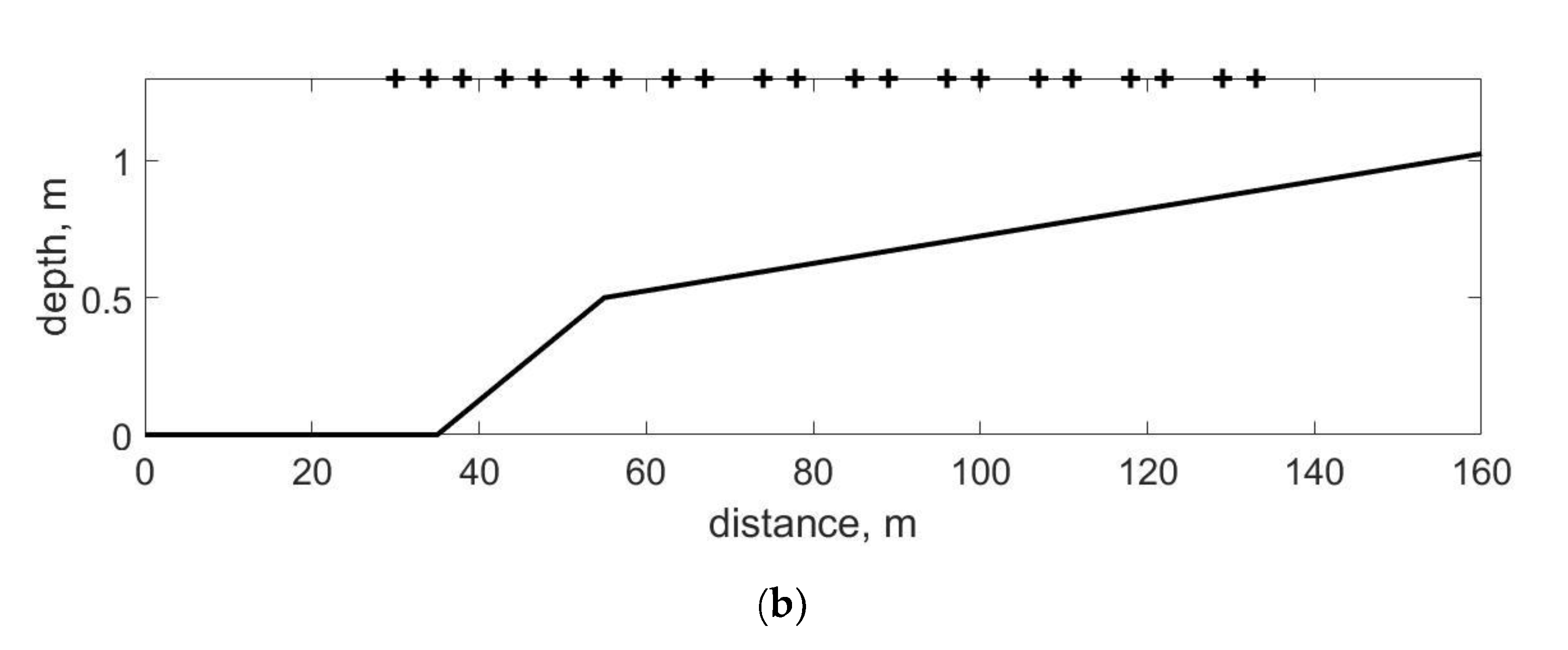
Various measurements are used to determine the change in wave parameters including satellites, radars, LIDARs, ADCPs, etc. However, the most informative from the point of view of the physical study of wave transformation are contact methods which obtain chronograms of individual waves by installing wave gauges (capacitive and resistance type wire gauges or pressure gauges on the bottom) or buoys. The classical spectra of spatial wave fluctuations in the theory of waves on deep water are constructed on the wavenumber. For the coastal zone, the length of which is less than 1 km, and some areas requiring study are even shorter. Therefore, typical spatial scales in coastal zones are from one to several wavelengths. It is not enough to construct reliably accurate wavenumber spectra. Therefore, the changes in wave parameters are estimated based on the spatial evolution of the wave frequency spectra obtained for each wave gauge. How wavenumber and frequency wave spectra differ and how they correspond to each other in determining the changing parameters of waves at decreasing water depths is not well understood.

A decrease of water depth leads to wave transformation and changes of its shape in space. Nonlinear features of wave transformation have been found in many fields, laboratory, and numerical experiments, but their physical interpretation is often difficult due to the lack of comprehensive theoretical solutions describing the transformation of waves under such conditions. The most popular is the theoretical approximation of long waves in shallow water for kh << 1 where h is the depth, k is the wavenumber, supposing that the waves propagate without dispersion. However, in most parts of the coastal zone, waves propagate at the so-called “intermediate depth,” when kh = O (1). As shown in [10], the evolution of such waves is associated with generation of nonlinear harmonics due to near-resonant three-wave (or triad) interactions:

$$\begin{array}{l}\pm k_1\pm k_2\mp k_3=\delta ,\\ \pm \omega {}_1\pm \omega {}_2\mp \omega {}_3=0,\end{array}$$

(2)

where ω = ω(k) is angular frequency connected with the wavenumber by dispersion relation for gravitational waves ω² = gk·tanh(kh), g is the acceleration of gravity, and δ is the detuning (or phase mismatch) arising from the impossibility to satisfy the conditions of full resonance (δ = 0) for this dispersion relation. 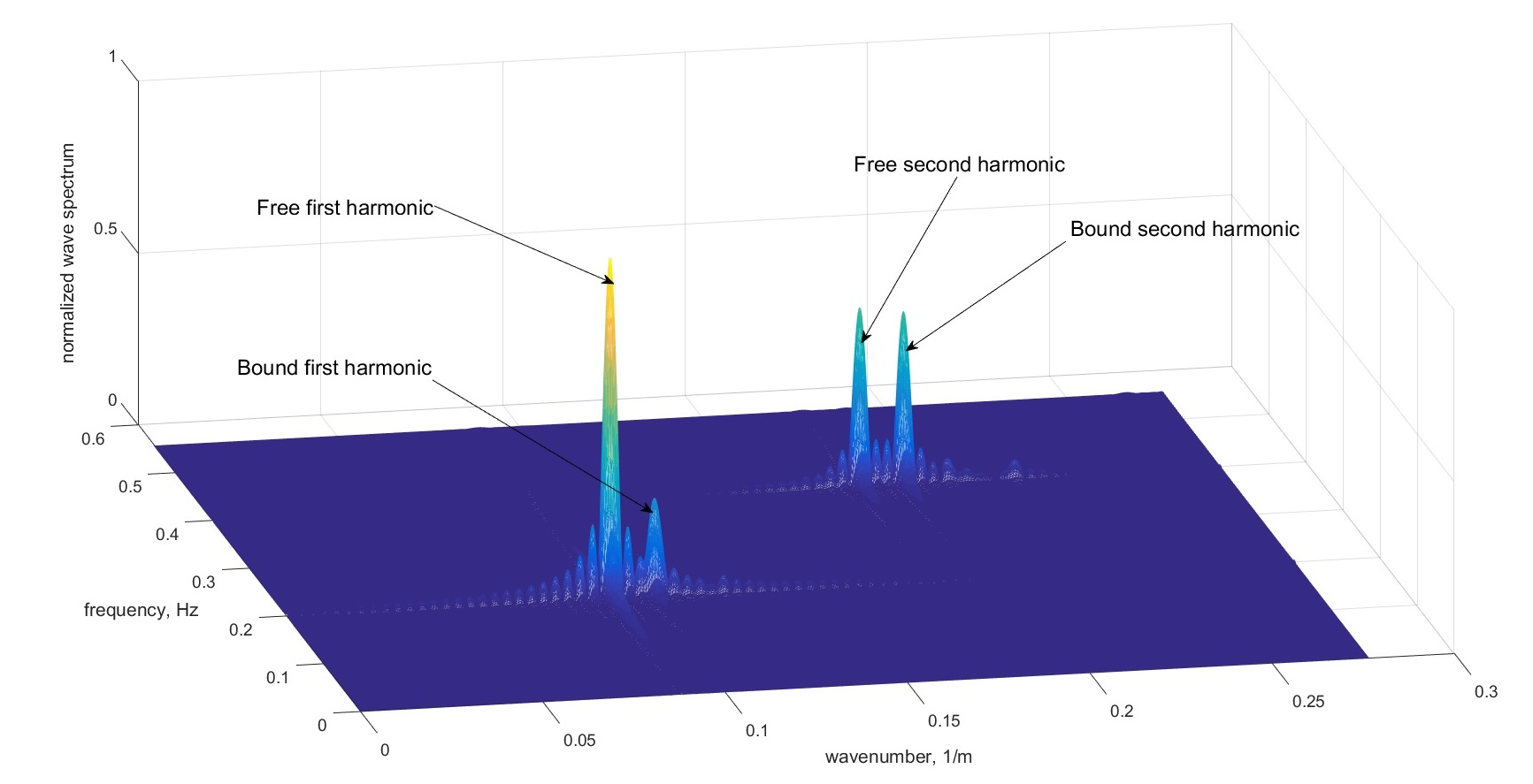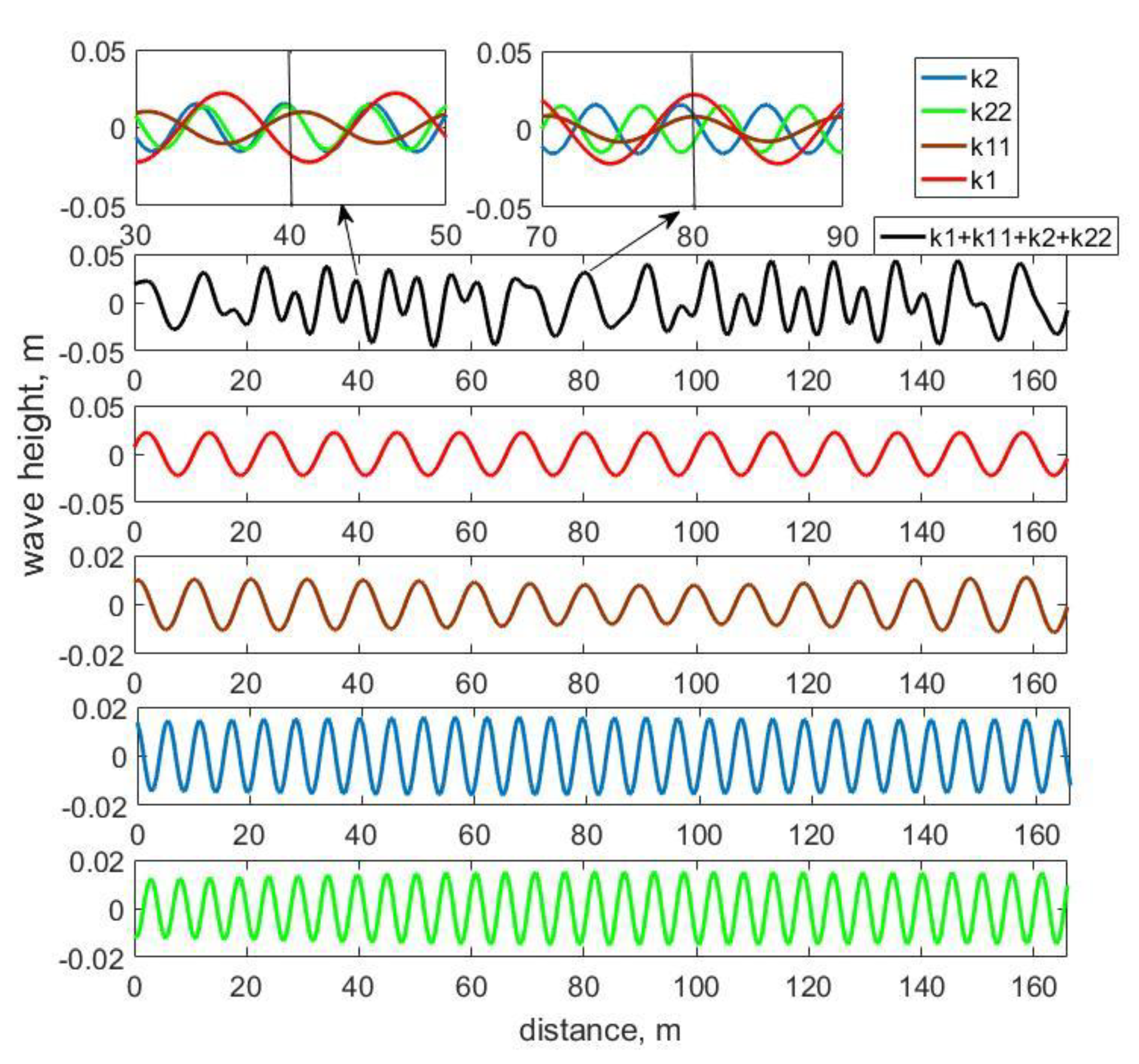If we consider the wave equation with first-order boundary conditions describing the propagation of waves at intermediate depth over the horizontal bottom, then we can obtain the solution [10] consisting of the first harmonic with constant amplitude and two second harmonics, free and bound, with doubled frequency of the first harmonic and the wavenumbers determined from the dispersion relation for the free harmonic and equal to the doubled wavenumber of the first harmonic:

$$S\left(x,t\right)=A_1\cos \left({\omega }_{1}t-k_{1}x\right)+A_2\left[\cos \left(2{\omega }_{1}t-2k_{1}x\right)-\cos \left(2{\omega }_{1}t-k_{2}x\right)\right]$$

(3)

where $t$ is a time, $x$ is a distance, and $A$ is constant amplitude coefficients depending on wavenumber and water depth. The superposition of free and bound second harmonics amplitude in frequency domain leads to spatial fluctuations of the wave amplitude. Theoretically, it was shown [10] that “free … second harmonic will interact with the primary wave to generate sum and difference frequency.” So, difference interactions between the free first harmonic of waves and the free second harmonic will generate the bound first harmonic with the same frequency as the free, but a different wavenumber.

In [10] the evolution equations, which numerically give solutions consisting only of bound harmonics in frequency domain with amplitudes slowly varying in space, were suggested also. Numerical solutions of these equations are in good agreement with the data of laboratory measurements [10].

It is obvious that the beats of the amplitudes of the harmonics slowly varying in space indicate the simultaneous presence of free and bound waves of both the second and the first harmonics. The beat spatial period, as well as the differences between the wavenumbers of free and bound waves, is determined by the mismatch δ:

$$\delta =k_2-2k_1$$

(4)

The use of second-order boundary conditions on the wavemaker (or initial conditions for the models) allows one to reduce the amplitude of the free second harmonic in some cases, but does not completely suppress them [10].

Many researchers in the laboratory and numerical experiments with mechanically-generated waves consider free waves of the second harmonic to be parasitic (or spurious) arising due to incorrect setting of the wavemaker moving in monochromatic manner and try to avoid them by the “correct” selection of initial conditions [10,11,12] according to the second order wave maker theory [13], because free waves make difficult the interpretation of the experimental results. Meanwhile, these “parasitic” free second harmonics also arise during the wave passing over an underwater bar in laboratory experiments or in nature when waves propagate over an inclined bottom [6,14].

A free second harmonic coincides with the bound ones when waves propagate without dispersion at very shallow water depths (kh → 0), when the detuning δ will be equal to zero (Formulas (2) and (4)). However, for real conditions of the coastal zone, taking into account the period of incident waves from 6 to 12 s, these depths will be less than half a meter.

The existence of space fluctuation of amplitudes of first and second frequency harmonics during wave propagation over inclined bottom in both field and laboratory conditions definitely confirms the simultaneous coexistence of free and bound waves.

The aim of the work is to demonstrate in detail the role of free and bound waves in the process of nonlinear wave transformation over an inclined bottom in intermediate water depth. For this, (1) a qualitative description of the physics and kinematics of the nonlinear process of wave transformation in the time and spatial domains will be given and (2) the important practical application of free and bound wave conception to explain visible paradoxes arising during the measurements of wave celerity and wave energy distributions across the coastal zone. The study is based on the data of field, laboratory, and numerical experiments and the methods of spectral and wavelet analyses.

2. Spatial Beats during Wave Transformation

2.1. Field Experiment

The main question is whether there are spatial beats in nature or if is it a theoretical result of near-resonance triad interactions of waves. Consider the data of the Shkorpilovtsi 2007 field experiment. During the experiment at the Shkorpilovtsi study site of the Institute of Oceanology of the Bulgarian Academy of Sciences, 15 wire wave gauges were evenly spatially located along the research pier (240 m) and installed at a depth range of 4.5−0.5 m. The free surface elevations at 15 points were synchronously measured at a sampling frequency of 5 Hz. The length of wave records was from 20 min to 1 h. A more detailed description of this field experiment and experimental results concerning irregular wave transformations can be found in [5,8,15,16,17].

Typical spatial evolution of the frequency spectrum of waves along the pier and the bottom profile are shown in Figure 1a,b. The spectra were estimated using Welch’s method with Hamming window.

The second nonlinear wave harmonics are clearly visible as a separate “ridge” (Figure 1a). The first harmonics are at the frequency of 0.12 Hz, the second at 0.24 Hz. Periodic fluctuations of harmonic amplitudes are clearly visible also: at the distance of 200 m from the coast, the second harmonic increases up to a maximum at a distance of 150 m and then decreases to a minimum at a distance of 100 m. The amplitude of the first harmonic fluctuates in antiphase with the amplitude of the second harmonic.

According to the data of this experiment, it was found that such a case of periodic energy exchange between the first and second nonlinear harmonics (or beat) is often observed during the transformation of waves on gentle slopes on the bottom. The criteria were obtained for the parameters of incoming waves and the bottom slope necessary for beat occurrence and the scenarios with the spatial beats and without them were classified [15]. The number of observed spatial periods of energy exchange between the first and second harmonics (beats) and the maximum second harmonic amplitude depends on the bottom slope and the wave steepness [15]. Thus, the periodic in space amplitude beats indicating the existence of free and bound waves harmonics during the transformation of irregular waves exist in nature. Based on this fact, we can note that in order to correspond to natural waves, waves mechanically generated under laboratory conditions must necessarily have some part of free waves at initial conditions.

Unfortunately, it is impossible to obtain the estimations of the wavenumber spectrum from the data of this experiment due to the small width of the coastal zone in relation to the wavelength and the insufficient number of measurement points required for good wavenumber spatial resolution.

2.2. Laboratory Experiment

A similar periodic exchange of energy between the first and second nonlinear harmonics is also observed for the spatial evolution of the frequency spectrum of initially monochromatic waves at their transformation over an inclined bottom in a laboratory experiment. The experiment was carried out in the Tainan Hydraulic Laboratory (Tainan, Taiwan) at 2015. Twenty-one wire capacitance type wave gauges were installed along the flume. The length of wave records was from 3 to 6 minutes with sample frequency of 50 Hz. The transformation of waves with an initial height of 5 to 40 cm and periods of 2 to 5 s were studied.

A typical evolution of the frequency spectrum of initially monochromatic waves of a 5-s period and 10-cm height is shown in Figure 2a. The bottom profile and location of wave gauges are shown at Figure 2b. The piston type wavemaker was at 0 m and net type wave absorber was at 160 m. Some additional details and other results concerning this experiment are in [8].

As in the case of irregular waves in field conditions, spatial beats or energy exchange between the first and second nonlinear harmonics fluctuating in antiphase are clearly visible. Figure 1a and a confirm the concept of wave transformation proposed in [10] that there is no frequency detuning, but there is a wavenumber detuning reflected in the spatial beats of the amplitudes of first and second nonlinear harmonics of the frequency spectrum.

2.3. Numerical Modelling, Monochromatic Wave

2.3.1. Inclined Bottom, Decreasing Water Depth

In the laboratory experiment, the number of wavelengths that fit into the wave propagation distance is greater than in the field experiment. However, as with the field experiment, we cannot estimate the wavenumbers spectrum with sufficient accuracy due to the small number of points for measuring waves in space. To obtain the evolution of waves in space with sufficient discretization, we will use Madsen and Sorensen’s model, based on the Boussinesq type equation with improved dispersion characteristics, which reproduces the beat effect [10,18]. As was suggested in [10], the Boussinesq-type equations were solved by a spectral modelling method in frequency domain. Compared to classical time domain modelling, spectral modelling is less time consuming and more accurate. In frequency domain, Boussinesq equations represent a set of evolution equations for complex Fourier amplitudes (А_р), total number of complex amplitudes and upper limit p depending on frequency discretization step.

$$\frac{d{A}_p}{dx}=-{\beta }_2\frac{h_x}{h}{A}_p-i2g(F_p^{+}+F_p^{-})-{\alpha }_n{A}_p$$

(5)

The first term of the right side of (5) describes the linear increase of amplitudes, h_x is slope steepness, h is water depth, and g is the gravitational acceleration. α_n is the dissipation rate, which is usually derived empirically and here we use frequency independent parametrization suggested in [18].

The second and third terms are, respectively, the summary and different triad interaction of harmonics, described by:

$$F_p^{-}={\displaystyle \sum _{m=1}^{\infty }\frac{{\alpha }^{-}}{{\beta }_1}}{A}_m^{*}{A}_{p+m}\exp [-i({\psi }_{m+p}+{\psi }_m+{\psi }_p)]$$

(6)

$$F_p^{+}={\displaystyle \sum _{m=1}^{p-1}\frac{{\alpha }^{+}}{2{\beta }_1}}{A}_m{A}_{p-m}\exp [-i({\psi }_m+{\psi }_{p-m}+{\psi }_p)]$$

(7)

where, β₁, α⁺ and α⁻ are interaction coefficients that depend on local depth (h), wavenumber (k_p), and angular frequency (ω_p). To save space, we do not show the formulas for β₁, α⁺ and α⁻ and α_n. They can be found in [10,18]. ψ_p is the phase, derived from

$$\frac{d{\psi }_p}{dx}=k_p$$

(8)

The evolution equations for wave amplitudes in the frequency domain were solved numerically by the fourth order Runge-Kutta method [10]. In the spatial domain, free surface elevations (waves) are obtained by the inverse Fourier transform:

$$\zeta ={\displaystyle \sum _{p=-\infty }^{\infty }{A}_p}(x)\exp [i({\omega }_{p}t-{\psi }_p(x))]$$

(9)

The spatial domain was from 0 up to 160 m with a spatial step of 0.1 m. The frequency step was 0.001 Hz.

The spatial evolution of initially monochromatic model waves with amplitude of 10 cm and a period of 5 s above the bottom relief in Figure 2b is shown in Figure 3a. The Morlet wavelet transform represents the evolution of wavenumber spectra during its propagation. It is clearly visible that as the waves are transformed due to decreasing water depth, the wavenumbers of both first and second wave harmonics change and, accordingly, the wave shape changes in space. If we consider the change of wavenumbers of first and second harmonics (Figure 3) over the length of one characteristic beat at evolution wave frequency spectra (from 50 to 90 m, Figure 2a), it can be seen that there are two close wavenumbers in the range (0.15–0.2 m⁻¹) (Figure 3b) corresponding to second harmonic in frequency wave spectra (Figure 2a) At distances up to 40 m, two wavenumbers are practically indistinguishable, since the amplitudes of the second harmonics are small. At distances of more than 90 m with decreasing of water depth, these wavenumbers change very quickly, and each wave (Figure 3a) has its own wavenumber of second harmonic. On wavelet transform (Figure 3b) the two wavenumbers in range [0, 0.1] for the first frequency wave harmonic at the distances 35 and 55 m can also be distinguished. However, its variability is not as strong as wavenumbers of the second harmonic. It is obvious that the wavenumbers of first and second harmonic are determined by the conditions of the “shallowness” of the water. The space-averaged wavenumber spectrum, for 30 seconds of wave evolution, confirms the presence of two wavenumbers for both the first and second harmonics (Figure 4).

2.3.2. Horizontal Bottom, Constant Water Depth

In order to evaluate in detail the evolution of the wave spectrum in terms of wavenumbers, to separate free and bound waves, and to compare the wave spectra in the frequency domain and in the wavenumber domain, avoiding the effect of decreasing depth, consider the propagation of this model monochromatic wave over a horizontal bottom with a constant water depth. At the depth of 0.5 m, this approximately corresponds to the conditions of wave transformation at a distance of 50 to 90 m, where the periodic energy exchange between harmonics in space (beat) was observed (Figure 2a). To study several exchange periods and have a good spatial resolution for the wavelength, we simulate the propagation of waves at a distance of 300 m (about 30 wavelengths) with the same frequency and space steps as in previous modelling.

The spatial evolution of the frequency spectrum of modelling waves demonstrates the presence in the frequency spectrum of waves of only two harmonics (first and second) and the period in space exchange of energy between them (Figure 5a). The time evolution of the spectrum of wavenumbers demonstrates the presence of four harmonics, two bound and two free (

Table 1. Wavenumbers and frequencies of harmonics.

Wave Harmonics	Wavenumber, 1/L, L–Wave Length (m−1)	Frequency, Hz
First free (k1, f1)	0.0885	0.2
First bound (k2–k1, f1)	0.0976	0.2
Second bound (2k1, 2f1)	0.1766	0.4
Second free (k2, 2f1)	0.1889	0.4

), with the constant amplitudes in time (Figure 5b). Constant and equal amplitudes of wavenumbers free and bound second harmonics in wavenumber domain correspond to Equation (3) in the introduction. The initial free first harmonic has a larger amplitude than the bound one arising as the result of difference interaction of free first and second harmonics. The interference of a wave of free and bound harmonics provides the space fluctuation of amplitude of first and second harmonics in frequency domain.

Wavelet analysis with Morlet wavelet function shows that as the waves propagate at the length of the characteristic beat, there are modulations of both the wavenumbers of the first and second nonlinear harmonics (Figure 6). The changes in the wave shape occur along the beat length; with the beginning of a new beat, the process is periodically repeated. The wavelet diagram shows that the amplitude of the wavenumbers of the first and second harmonics periodically fluctuate in space along the beat length.

Figure 6c shows the corresponding spatial changes of harmonic amplitudes. It is clearly seen that fluctuations of the wavenumbers of the first and second nonlinear harmonics correspond to the spatial periods of the beats of the frequency amplitudes (Figure 6c). However, as shown by the spectral analysis, the amplitudes of the wavenumbers do not change in time (Figure 5b)

On the base of wavenumber spectra, a linear filtration of the waves corresponding to all wavenumbers free and bound harmonics (Table 1) using the direct and inverse Fourier transform was carried out. It can be seen that fluctuations of the amplitudes of both the first and second harmonics at distance (in the spatial domain) are determined by the interference (or by the summation) of waves of wavenumbers of free and bound wave harmonics (Figure 7). The maximum amplitude of the frequency second harmonic corresponds to the superposition of two wavenumbers of second harmonic in phase (Figure 6c and Figure 7, distance 40 m), and the minimum to their change in antiphase ((Figure 6c and Figure 7, distance 80 m). Similarly, but in opposite phase, realized the interference of the two first harmonics. At the initial moment of time (t = 0), both of the second harmonics in wavenumber space have equal amplitudes and are in antiphase that corresponds theoretical assumption in [10].

Thus, the observed spatial beats or energy exchange between the first and second nonlinear harmonics are the result of the interference of free and bound waves with same frequencies, but different wavenumbers. There is no real exchange of energy between nonlinear harmonics. However, there are periodic fluctuations in the wave shape corresponding to the beat periods.

3. Discussion of Results

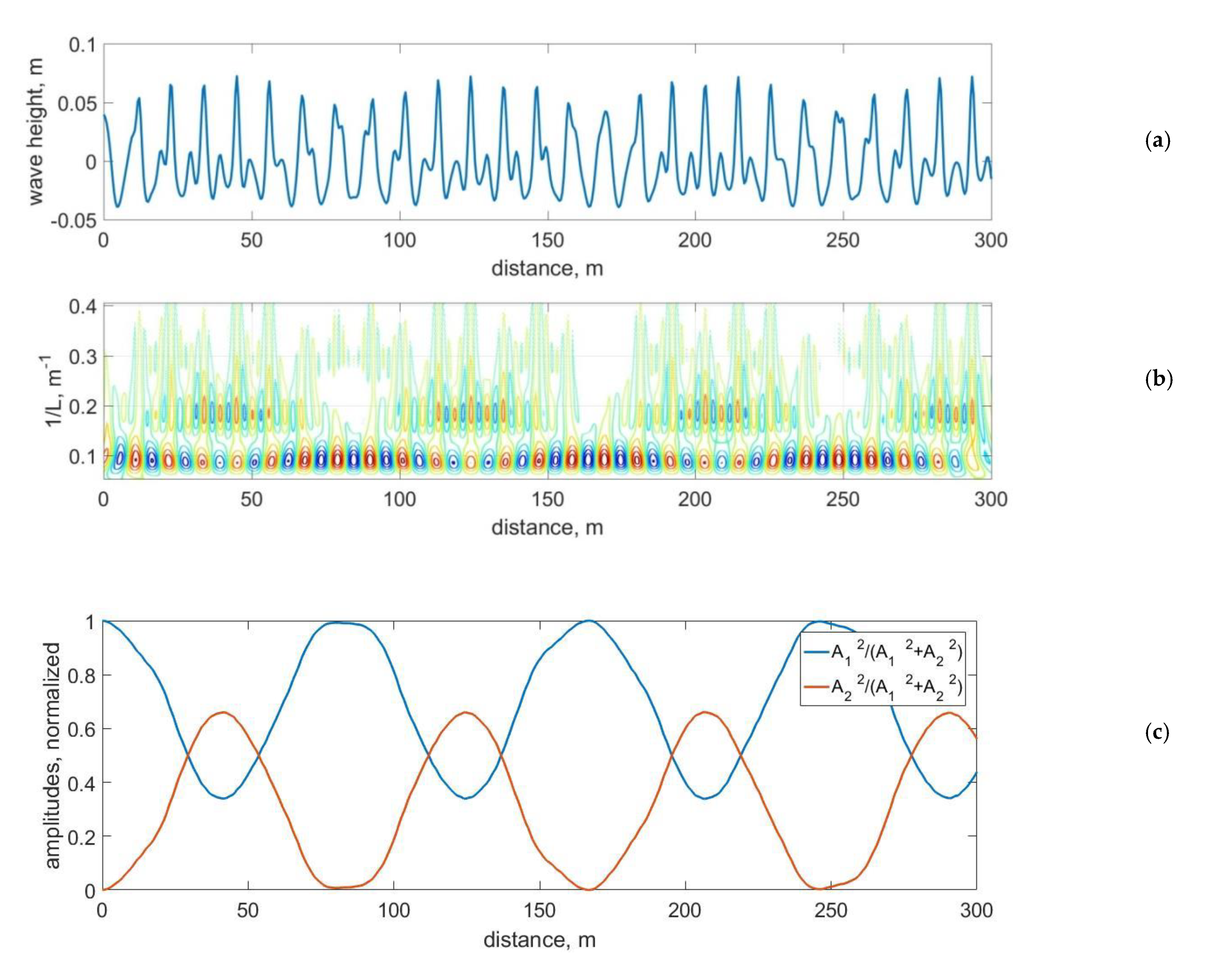
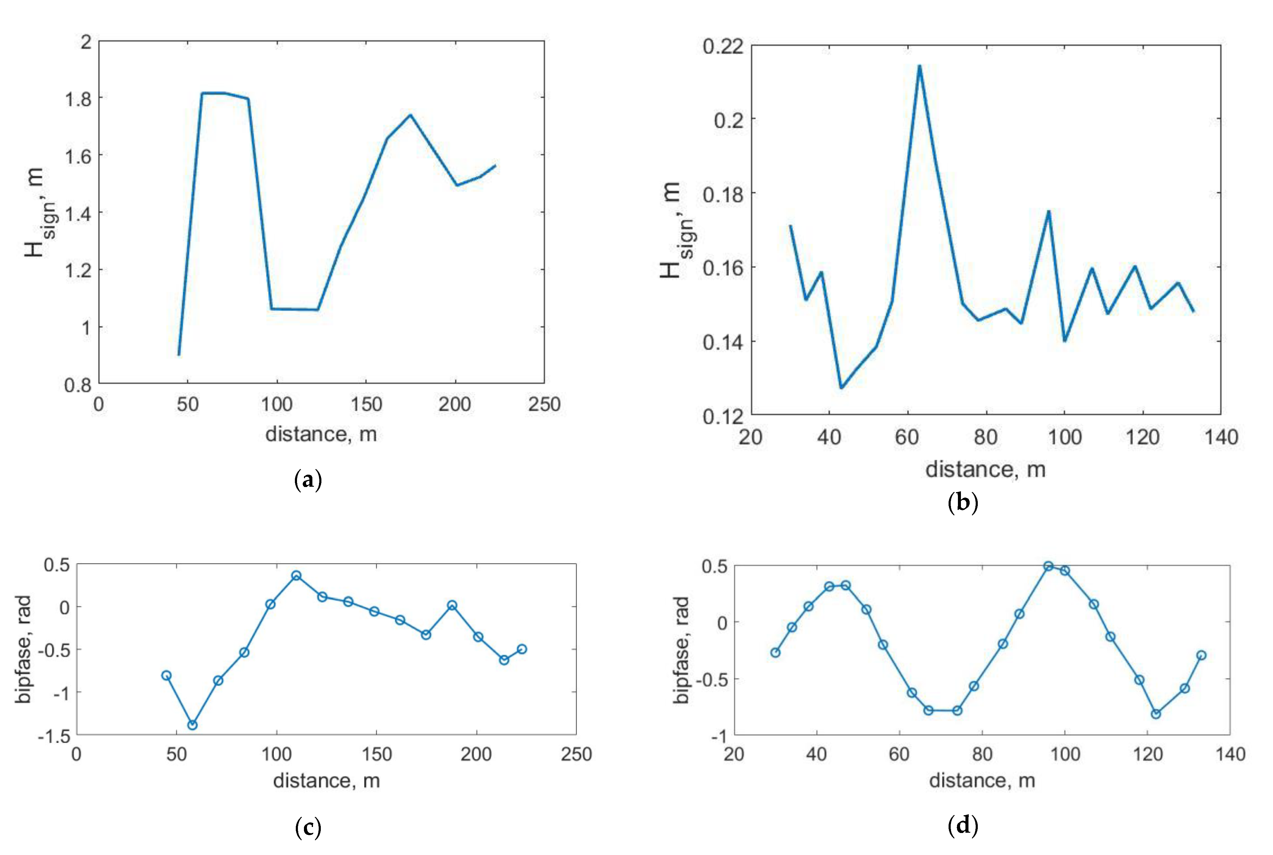
Significant nonlinear changes in the wave shape leads to various paradoxical results when the concepts of wave linear theory are applied to evaluate the characteristics of waves. So, for example, traditional estimates of the potential energy of waves from the point measurements proportional to the square of the significant wave height lead to unexpected fluctuations of the wave energy at different points of measurements that are inexplicable in the frame of the linear wave theory (Figure 8a). These fluctuations can be explained by the non-periodicity of the nonlinear wave motion, the waves at neighboring points in space differ significantly and it is impossible to replace the integration of the wave surface at its “length” by integrating the energy over the “period” of the wave at the point of measurement.

A similar effect of anomalous wave dispersion arises when estimating the phase velocities of propagation of nonlinear harmonics of waves from measurements at neighboring points [19]. Due to spatially periodic changes in the symmetry of the waves, the phase shift (biphase) between the first and second frequency harmonics also changes, as shown in Figure 8b for the discussed data of field and laboratory experiments. The biphase was calculated as was suggested in [20]:

$$\phi =\arctan \left[\frac{Im\left\{B\left({\omega }_1,{\omega }_2\right)\right\}}{Re\left\{B\left({\omega }_1,{\omega }_2\right)\right\}}\right]$$

(10)

where $B\left({\omega }_1,{\omega }_2\right)=E\left[A_{{\omega }_1}{A}_{{\omega }_2}{A}^{*}{}_{{\omega }_1+{\omega }_2}\right]$–bispectrum, ω–angular frequency, A–complex Fourier amplitudes of free surface elevations, E–averaging operator.

Fluctuations of the biphase shown in Figure 8 mean that the second harmonic is shifted forward relative to the first, then backward, which means that its phase velocity is sometimes greater and sometimes less than the phase velocity of the first harmonic.

A theoretical estimation of the phase shift between the first and second frequency harmonics can be obtained by reducing both terms of the second harmonic in Formula (3) to the form:

$$S\left(x,t\right)=A_1\cos \left({\omega }_{1}t-k_{1}x\right)+A_2\cos [2{\omega }_1+\pi /2-(k_1+k_2/2)x]\sin \left(k_2-2k_1\right)x$$

(11)

From (4), it is easy to obtain a biphase φ equal to the doubled phase of the first harmonic minus the phase of the second harmonic [20]:

$$\phi =-\frac{\pi }{2}+2\delta x$$

(12)

The biphase is equal to −π/2 at the initial moment of wave transformation and increases as the wave propagates, reaching 0 at the moment of the maximum amplitude of the second harmonic and continues to increase, which, taking into account the periodicity of trigonometric estimates, leads to fluctuations of the biphase in the range from −π/2 to π/2. This is clearly seen in Figure 8d.

4. Conclusions

It is shown that the space periodic exchange of energy between the first and second frequecy harmonics exist in the field condition where it arises naturally. According to the concept of free and bound waves, such periodical fluctuations are evidence of their existence.

It was revealed that observed spatial beats or energy exchange between the first and second frequency harmonics are the result of the interference of the free and bound harmonics in wavenumber domain. There are periodical fluctuations in the wave shape corresponding to length beat periods.

Numerical experiments of wave transformation over the constant depth have shown the existence of the bound first harmonic of waves, which has smaller amplitude than the first free one. At the same time, it should be noted the amplitudes of the free and bound second harmonics are equal.

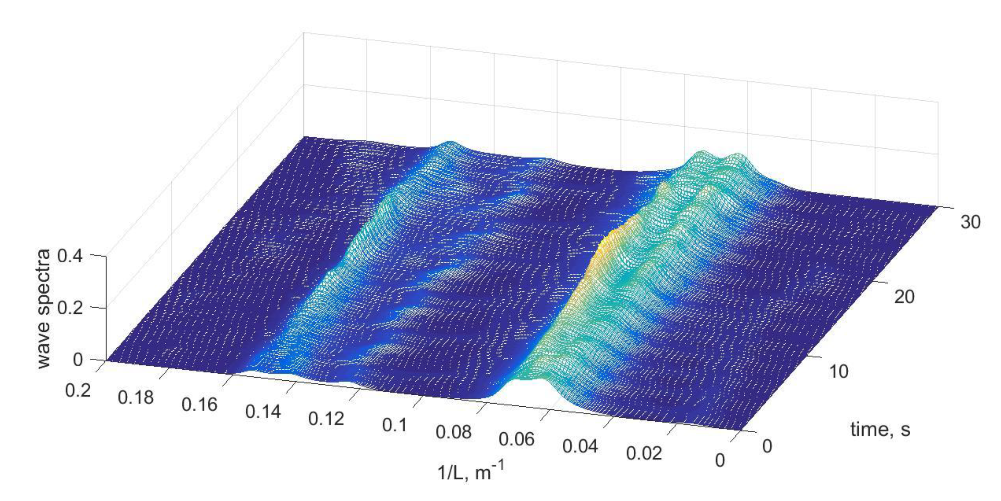
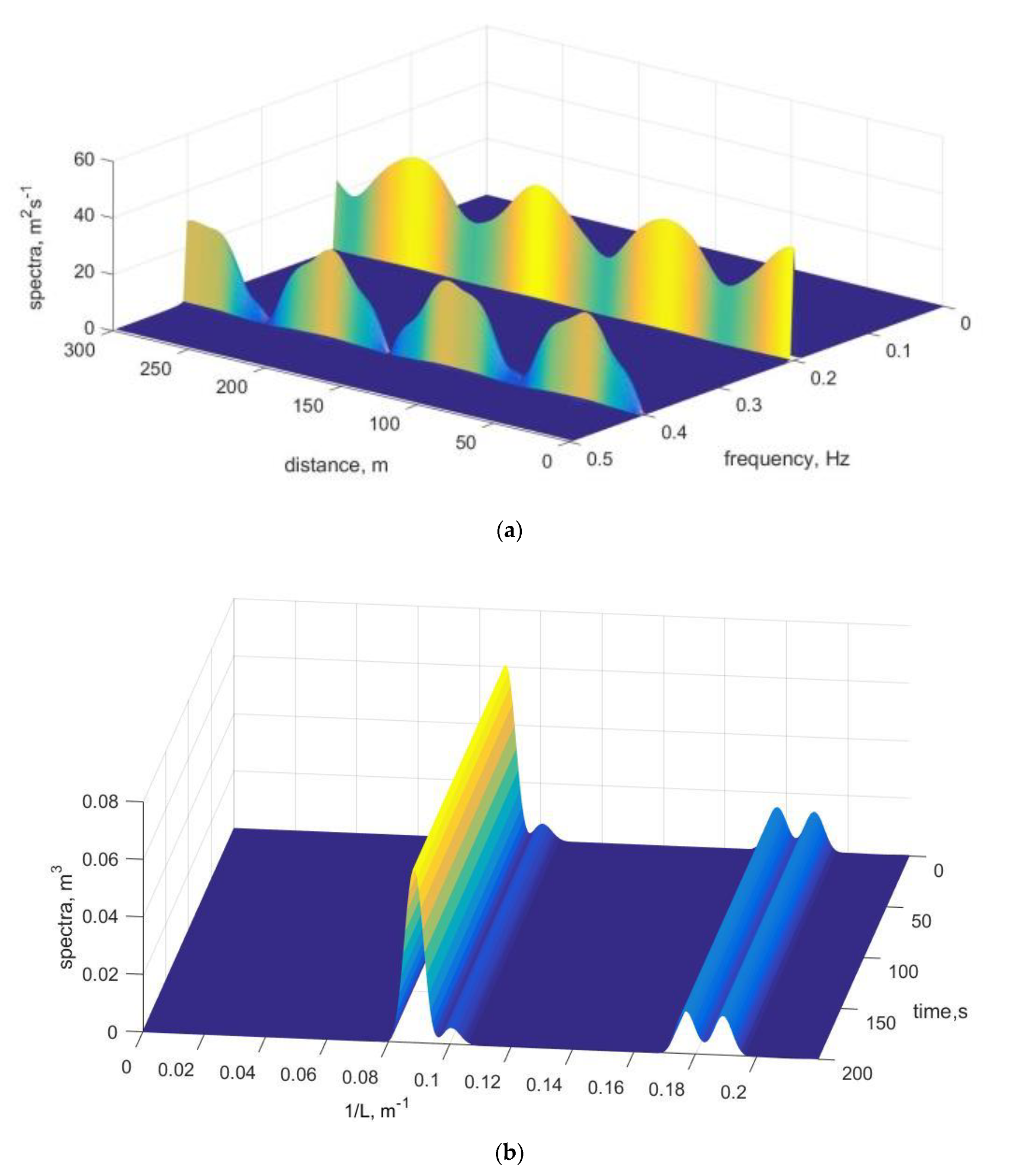
The difference between wave spectra on wavenumber and on frequency for the same wave field on intermediate and shallow water depth was investigated in detail.

When the spatial evolution of frequency spectra is analyzed, the effect of periodic energy exchange between the first and second harmonics of waves (beat) and changes in the phase shift between the harmonics in phase with the beat appear. When the wavenumber spectrum is analyzed, free and bound first and second harmonics with spatially invariable amplitudes are revealed, and all fluctuations of the wave parameters in space are caused by linear interference of these four harmonics.

There are observed fluctuations of the potential energy of waves and the appearance of anomalous dispersion (when the second harmonic celerity is higher than the first one) during the beat. These effects are the shortcoming consequences of the application of linear wave theory concepts of wave frequency and wavenumber to nonlinear waves and are important for estimating the wave parameters on the base of measurements in the coastal zone of the sea.

References

1. Hasselmann, K. On the nonlinear energy transfer in a gravity-wave spectrum. Part 1. General theory. J. Fluid Mech. 1962, 12, 481–500. [Google Scholar] [CrossRef]
2. Bailard, J. An energetics total load sediment transport model for a plane sloping beach. J. Geophys. Res. 1981, 86, 10938–10954. [Google Scholar] [CrossRef]
3. Stive, M.J.F. A model for cross-shore sediment transport. Coast. Eng. Proc. 1986, 1, 1550–1564. [Google Scholar] [CrossRef]
4. Boczar-Karakiewicz, B.; Davidson-Arnott, R.G. Nearshore bar formation by non-linear wave processes—A comparison of model results and field data. Mar. Geol. 1987, 77, 287–304. [Google Scholar] [CrossRef]
5. Saprykina, Y. The Influence of Wave Nonlinearity on Cross-Shore Sediment Transport in Coastal Zone: Experimental Investigations. Appl. Sci. 2020, 10, 4087. [Google Scholar] [CrossRef]
6. Kuznetsov, S.; Saprykina, Y. Secondary waves in coastal zone: Physical mechanisms of formation and possible application for coastal protection. Coast. Eng. Proc. 2012, 1, 12. [Google Scholar] [CrossRef]
7. Hulsbergen, C.H. Origin, effect and suppression of secondary waves. Coast. Eng. Proc. 1974, 1, 22. [Google Scholar] [CrossRef]
8. Saprykina, Y.V.; Kuznetsov, S.Y.; Kuznetsova, O.A.; Shugan, I.V.; Chen, Y.Y. Wave Breaking Type as a Typical Sign of Nonlinear Wave Transformation Stage in Coastal Zone. Phys. Wave Phenom. 2020, 28, 75–82. [Google Scholar] [CrossRef]
9. Paprota, M. Experimental Study on Spatial Variation of Mass Transport Induced by Surface Waves Generated in a Finite-Depth Laboratory Flume. J. Phys. Oceanogr. 2020, 50, 3501–3511. [Google Scholar] [CrossRef]
10. Madsen, P.A.; Sørensen, O.R. Bound waves and triad interactions in shallow water. Ocean. Eng. 1993, 20, 359–388. [Google Scholar] [CrossRef]
11. Orszaghova, J.; Taylor, P.H.; Borthwick, A.G.L.; Raby, A.C. Importance of second-order wave generation for focused wave group run-up and overtopping. Coast. Eng. 2014, 94, 63–79. [Google Scholar] [CrossRef] [Green Version]
12. Pierella, F.; Bredmose, H.; Dixen, M. Generation of highly nonlinear irregular waves in a wave flume experiment: Spurious harmonics and their effect on the wave spectrum. Coast. Eng. 2021, 164, 103816. [Google Scholar] [CrossRef]
13. Schäffer, H.A. Second-order wavemaker theory for irregular waves. Ocean. Eng. 1996, 23, 47–88. [Google Scholar] [CrossRef]
14. Li, F.C.; Ting, C.L. Separation of free and bound harmonics in waves. Coast. Eng. 2012, 67, 29–40. [Google Scholar] [CrossRef]
15. Saprykina, Y.V.; Kuznetsov, S.Y.; Shtremel, M.N.; Andreeva, N.K. Scenarios of nonlinear wave transformation in the coastal zone. Oceanology 2013, 53, 422–431. [Google Scholar] [CrossRef]
16. Saprykina, Y.V.; Kuznetsov, S.Y.; Divinskii, B.V. Influence of processes of nonlinear transformations of waves in the coastal zone on the height of breaking waves. Oceanology. 2017, 57, 383–393. [Google Scholar] [CrossRef]
17. Saprykina, Y.V.; Shtremel, M.N.; Kuznetsov, S.Y. On the possibility of biphase parametrization for wave transformation in the coastal zone. Oceanology 2017, 57, 253–264. [Google Scholar] [CrossRef]
18. Eldeberky, Y.; Battjes, J.A. Spectral modeling of wave breaking: Application to Boussinesq equations. J. Geophys. Res. 1996, 101, 1253–1264. [Google Scholar] [CrossRef]
19. Кuznetsov, S.Y.; Speransky, N.S. Anomalous dispersion paradox in shallow water gravity waves shoaling over slopping bottom. In Proceedings of the 2nd International Symposium on Ocean Wave Measurement and Analysis, New Orleans, LA, USA, 25–28 July 1993; American Society of Civil Engineers: Reston, VA, USA, 1994; pp. 364–373. [Google Scholar]
20. Kim, Y.C.; Powers, E.J. Digital bispectral analysis of self-excited fluctuation spectra. Phys. Fluids 1978, 21, 1452. [Google Scholar] [CrossRef]
Figure 1. Periodical in space fluctuations of wave frequency spectrum normalized on wave dispersion (a) over the bottom profile (b). Field experiment Shkorpilovtsi 2007, series 62, o–positions of wave gauges.
Fluids 06 00347 g001
Figure 2. Periodical in-space fluctuations of wave frequency spectrum normalized on wave dispersion (a) over the bottom profile (b). Fiel Laboratory experiment Tainan 2015, series 41, +—positions of wave gauges.
Fluids 06 00347 g002aFluids 06 00347 g002b
Figure 3. Spatial evolution of initially monochromatic wave (a) and its wavelet transform (b) modelled for the bottom relief in Fig. 2b. Wavelet coefficients are shown by the intensity of the color from dark blue (minimum) to dark red (maximum).
Fluids 06 00347 g003
Figure 4. Evolution of wavenumber spectra of model monochromatic wave in time above bottom relief Figure 2b.
Fluids 06 00347 g004
Figure 5. Frequency (a) and wavenumber spectra (b) of model monochromatic wave propagated over constant depth of 0.5 m.
Fluids 06 00347 g005
Figure 6. Spatial fluctuations of amplitudes of first and second harmonics of model monochromatic waves propagated over a constant depth of 0.5 m. (a) waves evolution with distance, (b) its wavelet transform, (c) fluctuations of frequency amplitudes corresponding Figure 5a.
Fluids 06 00347 g006
Figure 7. Demonstration of interference of waves corresponding free and bound waves of wave harmonics of model monochromatic wave propagated over constant depth 0.5 m.
Fluids 06 00347 g007
Figure 8. Spatial fluctuations of significant wave heights (a,b) and biphase (c,d) in field (a,c) and laboratory (b,d) experiments.
Fluids 06 00347 g008