Abstract
A multiscale dynamic analysis of the commutation error, based on the filtering approach is performed. The similarity multiscale hypothesis proposed by Bardina (1983) and extended by Geurts and Holm (2006) to the commutation error is examined in detail and an extension of the Germano identity to the analysis and the modelling of the commutation error is proposed. For a detailed analysis under controlled condition the method is first applied to synthetic turbulence and subsequently to the a-priori analysis of a turbulent channel flow at . The results illustrate the flexibility of the dynamic modelling approach. Combined with a scale similarity assumption for the commutation error very satisfactory results have been obtained for first order derivatives and reasonable results for second order derivatives. In all cases the modelling of the commutation error resulted in smaller errors than the error obtained by neglecting the commutation error.
1. Introduction
Turbulence modelling using the Large Eddy Simulation (LES) technique is considered advantageous over traditional methods relying on Reynolds averaging due to its inherent ability to resolve the energy carrying turbulent structures. Given the advances in computing power over the last decades, together with recent advances in numerical methods [1,2] and advanced modelling techniques [3,4] based on machine learning, it can be expected that LES will be increasingly used in the future for a variety of applications such as combustion [5,6] or two-phase flows [7,8,9] to name only two.
The Large Eddy Simulation of turbulent flow is affected by many errors, due to many reasons, first of all the granularity of the grid coupled with the nonlinearity of the equations. Following Reference [10], we can formalize all that in terms of a filtering approach that reads the data produced by a numerical code as a filtered database. The filtering operator representative of a given LES is characterized by a filter length, directly associated to the grid length, and a lot of information, useful both for modelling and for analysing the results, can be recovered by comparing two different simulations at two different resolution levels by means of the so called dynamic filtering approach. As recalled in the abstract, the first application of the dynamic modelling approach was presented thirty years ago at the Summer Meeting of the CTR [11], and since then a lot of different applications flourished thanks to the interest of many researchers around the world. We refer both to the cited Reference [12] and to Reference [13] for more details on that.
In order to derive the LES formalism, the Navier-Stokes equations are usually filtered with a commutative filter, that is, where u denotes a general variable and a general filtering operation, typically defined as a convolution integral (here for illustration in 1D) with the filter kernel G such that
Examples of filter kernels in physical scace are the box filter
or the Gaussian filter
Making use of the linearity of filtering one obtains
Without loss of generality viscosity and density are assumed to be constant. Two approaches exist to deal with the unknown correlation appearing in the filtered Navier-Stokes equations [14]:
The term in parentheses is the unknown sgs stress tensor . If Equation (5) is used, a closed equation for is obtained, provided a model for is supplied. This equation requires no explicit filtering during the solution process. If relation (6) is used one obtains again a closed equation but this time with an additional explicit filtering operation applied to the non linear term. Therefore we call the first approach implicit filtering and the second approach explicit filtering ([15] uses the terminology triple and double decomposition).
In order to derive Equation (4) a homogeneous filter defined in an infinite domain has been assumed. Problems with the theory outlined so far can therefore arise from inhomogeneous filters or from bounded computational domains. This can be seen by differentiating Equation (1) with respect to x which gives [15]:
Inhomogeneous filters (grids) are extensively applied in the proximity of walls or regions of strong gradients, like shear layers for example. Hence, the commutation of derivation and filtering is of particular importance for manipulating the Navier-Stokes equations and application of a non commutative filter to the governing equations results in unknown expressions for all terms.
The problem of deriving high order commutative (HOC) filters has been addressed in the past literature (e.g., References [16,17,18]). Vasilyev et al. [17] developed a class of HOC filters using a mapping function. In extension to that work Marsden et al. [18] proposed a more general procedure for use on unstructured meshes. These filters are defined as a linear combination of simple commutative basis filters, thus allowing to control additionally the filter shape. An implementation of this method into an unstructured solver can for example be found in Reference [19]. The underlying idea of the work mentioned above is that the commutation error can be controlled by imposing conditions on the filter moments. However, as the primary filtering operation is not explicitly performed in a real LES [14], a general limitation of these ideas is, that these commutative filters can only be used for the secondary filtering operation, such as in Equation (6), or when using a test filter in the dynamic modelling approach. John [20] argues that the commutation error vanishes if and only if the normal stress on the boundary is zero for all times which is very unlikely. While the analysis in this work considers only spatial, time independent filters, it is worth to mention the following extensions: Leonard et al. [21] discuss the commutation error when the spatial filter varies in time, while Franke and Frank analyse the temporal commutation error [22]. The next sections discuss a framework that potentially could be used for modelling the commutation error for the primary filtering operation such as in Equation (5).
2. Multiscale Modelling
It has been mentioned in Reference [23] that the commutation error can be modelled using a scale similarity type approach. Here the main attention is not only to modelling but equally important to analyse the commutation errors with the filtering approach and the related multiscale procedure based on the Germano identity. We remark that in the framework of the filtering approach a Large Eddy Simulation of a turbulent flow is mathematically formalized as a filtered representation of a Direct Simulation. If with we represent the filtering operator usually unknown and denoted with an overbar , that produces the filtered LES values of the velocity components, a basic problem is to understand how the filtered product is related to them. The filtering approach tries to resolve this problem from a multiscale point of view. We define the Generalized Central Moment, (GCM), associated to as
and we look to the GCM associated to , where is an explicit test filtering operator, denoted also with a hat ,
It is easy to see that the resolved GCM (based on resolved quantities and considering filter level g),
can alternatively be expressed by the tensor defined as
Inserting a model expression for and with one free model parameter into Equation (11) to express and equating it to Equation (10) one could in principle determine this model parameter from
However, each tensor component would provide a different equation and a different value of for the model parameter. If instead we contract the identity Equation (12) with , following the approach of Lilly [24], we have identically
The contraction corresponds to summation over both indices and as a result of it the resulting model parameter represents the single model parameter which provides the best approximation in a least square sense to the six equations representing the symmetric tensor components.
We remark that from the LES modelling point of view, but not only, it is very important to understand how the dynamic coefficient C
scales with resolved quantities. Obviously the dynamic coefficient C should be rigorously equal to one everywhere if the modelling scaling is exact, but this is not the case for a generic scaling model. As an example, we can scale with the similarity model of Bardina [25].
Thus we can write
and finally the parameter be computed with resolved quantities
where
In this local form, the Bardina dynamic coefficient depends on time and space, but a global form can be conceived, averaged in time and/or eventually in homogeneous space directions.
Strangely enough this multiscale approach and the main use of the identity Equation (12) was to model turbulence, and not to analyse its multiscale peculiarities. The reasons for that are not so simple to explain. We only remark that this attitude has prevented simple observations that could be usefully applied to LES. One of them refers to the commutation error, and that is the main contribution of this paper. Let us formally consider the GCM associated to the filtered product of a space derivative with a velocity component , on filter level defined as
If we introduce once more an explicit test filter , a simple extension of the identity Equation (12) is the following
where is the resolved GCM given by
We can contract this identity like
where
and also in this case it is very important to understand how the dynamic coefficient C associated to the commutation GCM,
scales with resolved quantities. Obviously the candidates to this explorations are many. The scale similarity model is known to show high correlations in a-priori tests not only for isothermal flows but also for the stress, the flux modelling and the reaction rate closure in reacting flows [26,27,28] or two phase flows [7,8]. The problem of insufficient dissipation of the model has for example been addressed in Reference [29]. Encouraged by these results and by the work of Reference [23] we will therefore examine in some detail how the ratio C scales with the extension of the similarity model of Bardina [25]. We write
as well as
such that finally
where numerator and denominator will be space or ensemble averaged as appropriate. Averaging is a standard procedure for regularisation of the dynamic procedure (for an overview on this topic see Reference [15]). For unsteady 3D flow problems the averaging in homogeneous directions can be replaced by the Lagrangian dynamic model proposed by Meneveau et al. [30].
3. Approximations for Commutation Errors
In this section a first order approximation of the commutation error for the first and second derivative will be presented under the assumption that the filter is a differential or elliptic filter. If the filter varies in space and the filter width is formally associated to the length scale one can explicitly include this dependency in Equation (7)
such that the commutation error can be formally expressed in one dimension as [31,32]
By using the overline notation we derive the following expression for the second order derivative
The commutation error has been also examined in Reference [33]. From this last paper we can derive an estimate of the derivative of with in the case of the elliptic differential filter [34]
In this case we have as a first approximation
Similarly, the Gaussian filter and its inverse can be approximated by a differential filter [15]
If, using Equation (34), we write as a first approximation
the first term to the right in Equation (39) reads as
One can assume that and . Often a constant grid stretching is used such that and . Under these conditions one has
4. Analysis of Synthetic Turbulence
The commutation for the primary filter affects, apart from the temporal derivative, every term in the Navier-Stokes equations. Hence an implementation of the methodology in a real LES will be cumbersome and not straightforward on bounded domains with non-uniform meshes. For a first illustration of the methodology a simple 1D example has been chosen here, which has also the advantage that all turbulence parameters can be strictly controlled.
4.1. First Order Derivatives
The computational mesh used for illustration of the method is a stretched one-dimensional mesh with variables stored in the cell center on a domain with unity length. The first cell has a length of and the subsequent cells (50 in total) have the width where s is a constant stretch factor taken as for the example in Figure 1. In this particular case the first mesh cell has a width of . The discrete filter is an inhomogeneous, asymmetric box filter as illustrated in Figure 1.

Figure 1.
Illustration of the stretched 1D computational mesh with cell centred data storage and one sketched box filter.
For a given parameter p the filter around a point is given by the coefficients with the weights :
All derivatives are calculated by second order accurate finite differences for non-equidistant meshes
where denotes the midpoints of the cells. It is worth noting that this formula reduces to the standard central difference for equidistant meshes. Due to the inhomogeneous filtering operation the mesh has to be elongated in positive and negative direction in order to have a well-defined filtering operation for up to fourfold filtering. Pseudo turbulent data has been generated using the digital filter based method detailed in Reference [35], where the integral turbulent length scale has been set to respectively and the fluctuation intensity is set to unity without loss of generality. The associated two-point autocorrelation function (an equivalent of the energy spectrum) obtained by this approach resembles homogenous isotropic turbulence in a late stage [35].
The turbulent initial data has been generated on a uniform mesh and interpolated on the non-equidistant computational mesh using a cubic spline function, as illustrated in Figure 2. The derivatives of the signal shown in Figure 2 and the associated commutation error are shown in Figure 3a,b. It is worth noting that for a homogeneous symmetric filter and this has been verified in the numerical implementation by setting the stretch factor to . We remark that the numerical gradients become smaller with larger grid size (i.e., towards the right boundary of the computational domain). The scale similarity model given by Equation (25) is shown together with the commutation error in Figure 3b using . Table 1 shows the performance of the model in terms of the Pearson correlation coefficient for initial data with two different length scales and two different filter width, which according to Equation (43) can be specified using the parameter . Furthermore, Table 1 shows the optimal model parameter C determined from a least square fit of the model data to the real commutation error according to Equation (25). The numerical experiment has been repeated 2000 times and all data is space and ensemble averaged. In a real LES determination of the model constant C using least square fits is not possible because the commutation error is unknown. Table 1 shows also the dynamically determined model coefficient for different initial data and different filter size pairs . It can be seen that the dynamic procedure reasonably represents the optimal model coefficient. It is also worth mentioning that in all cases the model error, using either the default value or the optimal value from least square fits, has been found to be considerably smaller than the commutation error (representative of using no model) and this is demonstrated in Table 1 by the relative mean squared error (RMSE) defined as the local mean squared commutation error divided by the local mean squared value of the derivative of the signal multiplied with 100. We remark the simple extension of the dynamic procedure that can be easily generalized and implemented in different directions.
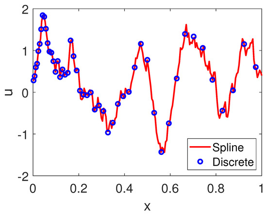
Figure 2.
Spline through digital filter based pseudo turbulence and corresponding values interpolated on the computational mesh.
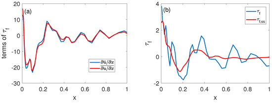
Figure 3.
(a) (Filtered) gradients of the data (filtered data) shown in Figure 2. (b) Commutation error given by together with scale similarity model for the commutation error, given by Equation (25) using .

Table 1.
Performance of model for different initial data and different filter sizes (note that the correlation coefficient is independent of the secondary filter). Dynamically determined model coefficient C and mean squared error between commutation error and different approximations, for different initial data and different filter size pairs .
4.2. Second Order Derivatives
The same procedure can be automatically extended to the second derivatives. The commutation error is then given by:
The second numerical derivatives are calculated using the following formula:
The scale similarity model for the second derivative reads:
The associated filtered second derivatives and second derivatives of filtered data are illustrated in Figure 4a. The scale similarity model given by Equation (47) is shown together with the commutation error in Figure 4b using . It becomes immediately clear that the scale similarity assumption works less satisfactory for the second derivative compared to the first derivative. Selected results for the second derivatives are summarised in Table 2. The modelling and dynamic procedure are in analogy to the case of the first derivative.
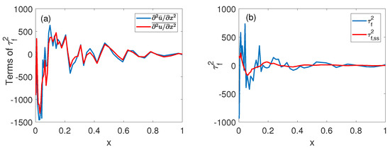

Table 2.
Performance of model for different initial data and different filter sizes (note that the correlation coefficient is independent of the secondary filter). Dynamically determined model coefficient C for different initial data and different filter size pairs .
While the correlation strengths for the second derivatives are lower compared to the first derivative and also the reduction of RMSE happens to a smaller extend, Table 2 still shows that modelling the commutation error results in a smaller error compared to the commutation error itself especially for small filter width pairs .
5. Analysis of Turbulent Channel Flow at
Next the relations from Section 2 will be applied to DNS data. For this a-priori analysis a turbulent channel flow DNS at is considered. The equations are solved by using a finite volume technique on a cartesian mesh. The variables are located on a staggered grid. For spatial discretization second order central differences are used. Temporal discretization is an explicit third order, Runge–Kutta-method. The Poisson equation is inverted by using a direct fast solver.
For the channel flow DNS the Reynolds number, based on the wall friction velocity, has been set to similar to the DNS data of Moser et al. [36]. The extension of the computational domain in axial spanwise and vertical direction is where is the channel half width. The computational domain is resolved with grid points. The grid is stretched in wall normal direction with a factor of such that and . A fixed theoretical pressure gradient is prescribed in the simulations. This results in a mesh of dimensions in the channel center and at the wall. The filter width parameter has been chosen to for the primary filter and for the test filter. To avoid ambiguous definitions of the filter when approaching the wall, all filtering operations stay away from the wall such that with every filter operation the signal becomes a little bit shorter. Nevertheless, for the analysis presented here this is entirely irrelevant. Periodic boundary conditions are applied in axial and spanwise direction, no slip conditions at the wall. It is worth noting that the above mesh can be considered typical for a channel flow DNS. Using the filter parameter , that is, combining three neighbouring cells into a representative filter volume, can be considered typical for a wall resolved LES mesh. The meshes in homogeneous -directions of channel flow LES/DNS are typically uniform and no commutation errors occur in this direction. Therefore only selected z-components of the different terms of the Navier-Stokes equation have been analysed. It is remarked that in contrast to the analysis in Section 4 where mean values of the signal were zero, the mean axial velocity profile for a channel flow is characterised by strong wall normal gradients in particular in the vicinity to the wall. In other words the signal to be analysed contains the mean velocity contribution which makes it more predictable. Furthermore it is remarked that the wall normal filter width for the DNS and the a-priori LES analysis is very small, presumably much smaller than characteristic turbulent length scales.
First attention is focused on the first order derivatives in the Navier-Stokes equation, that is, the convective term and the pressure gradient. Figure 5a compares the commutation error for the wall normal derivative of convective component with the wall normal gradient of the SGS turbulent flux. Consistent with the analysis of Reference [37] it is found that the commutation error for the convective term can have the same order of magnitude than the SGS contribution. It can further be seen from Figure 5b,d that the scale similarity model represents very well the commutation errors for the term and the pressure gradient, where the commutation error for the pressure gradient is much smaller in magnitude. Finally, Figure 5c shows that the dynamically determined model parameter is very close to unity which is consistent with subfigure (b). It is argued that this result is due to the small wall normal filter width (typical for wall bounded LES/DNS) and the velocity profile being dominated by the strong mean gradients.
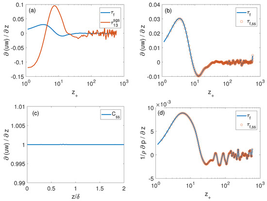
Figure 5.
(a) Commutation error at primary filter level f for the first derivative compared to the SGS component . (b) Commutation error at primary filter level f for the first derivative together with the corresponding scale similarity model. (c) Dynamic model parameter averaged in both homogeneous directions. (d) Commutation error at primary filter level f for the pressure gradient together with the corresponding scale similarity model. Without explicitly mentioning it, all results have been averaged in both homogeneous directions here and in the following figures.
Terms containing second derivatives, that is, for constant viscosity and density flow the diffusion term and the pressure Laplacian appearing in the Poisson equation for the pressure, will be considered next in Figure 6. Subfigure (a) again shows a very good performance of the scale similarity model (here for the second derivative). Similar observations in regards of the performance for the pressure Laplacian can be seen in Figure 6b. In all cases shown in Figure 5 and Figure 6 the optimal model parameter is very close to unity which has been recovered by the dynamic procedure, but is not explicitly shown here for all terms.
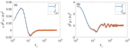
Figure 6.
(a) Commutation error at primary filter level f for the second derivative (viscous term) together with the corresponding scale similarity model. (b) Commutation error at primary filter level f for the second derivative appearing in the Poisson equation of the projection method together with the corresponding scale similarity model.
6. Conclusions
A large eddy simulation consists of filtering the Navier-Stokes equations in order to compute the large energy carrying motions of the flow while the smaller scales are modelled. The scale separation is formally introduced by a filtering operation. While this approach is very appealing, the filtering operation turns out to be more difficult compared to Reynolds averaging, because of the non-commutativity non only with respect to products but also with respect to derivatives in the case of anisotropic meshes.
A dynamic commutation error model has been produced by generalizing the dynamic modelling procedure. The commutation errors at two different resolution levels are defined and a multiscale identity relating them is derived. All that is in strict analogy with the well known dynamic model. The first results are promising for the future and it is remarked that the same formalism has been extended to second derivatives as well. The framework has been first applied to a synthetic turbulent flow with zero mean values and precisely controllable turbulence characteristics. The results reveal a good correlation strength of the scale similarity model and the dynamic procedure was shown to provide model coefficients close to the optimal model parameter (which cannot be calculated in a real LES in the absence of DNS data).
In a second step an a-priori analysis of a turbulent channel flow has been conducted indicating that the scale similarity models provide a very satisfactory performance with optimal model parameters very close to unity, which again was reproduced by the dynamic procedure. Selected terms of the Navier-Stokes equations have been analysed, showing that the commutation error for the first and second derivative can have a similar order of magnitude than the convective SGS contribution, which is (for the first derivative) consistent with findings from Reference [37] for a different flow configuration and different filtering technique.
In particular the results show, as remarked by Reference [12] that constraints derived from generalizations of the multiscale identities between different resolution levels may provide useful input in the specification of model parameters. Apart future more dedicated applications, the main aim of this short note should be to show the easiness and flexibility of the dynamic approach in very different modelling contexts.
Author Contributions
Conceptualization, M.G. and M.K.; methodology, M.G.; software, M.K.; formal analysis, M.K.; writing—original draft preparation, M.K. and M.G.; writing—review and editing, M.K. and M.G.; visualization, M.K. All authors have read and agreed to the published version of the manuscript.
Funding
This research received no external funding.
Institutional Review Board Statement
Not applicable for studies not involving humans.
Informed Consent Statement
Not applicable for studies not involving humans.
Data Availability Statement
Data available on reasonable request from the authors.
Conflicts of Interest
The authors declare no conflict of interest.
References
- De Wiart, C.C.; Hillewaert, K.; Bricteux, L.; Winckelmans, G. Implicit LES of free and wall-bounded turbulent flows based on the discontinuous Galerkin/symmetric interior penalty method. Int. J. Numer. Methods Fluids 2015, 78, 335–354. [Google Scholar] [CrossRef]
- Creech, A.; Jackson, A. Hybrid Large Eddy Simulation for low-order Discontinuous Galerkin methods using an explicit filter. Comput. Phys. Commun. 2021, 260, 107730. [Google Scholar] [CrossRef]
- Schoepplein, M.; Weatheritt, J.; Sandberg, R.; Talei, M.; Klein, M. Application of an evolutionary algorithm to LES modelling of turbulent transport in premixed flames. J. Comput. Phys. 2018, 374, 1166–1179. [Google Scholar] [CrossRef]
- Reissmann, M.; Hasslberger, J.; Sandberg, R.D.; Klein, M. Application of Gene Expression Programming to a-posteriori LES modeling of a Taylor Green Vortex. J. Comput. Phys. 2021, 424, 109859. [Google Scholar] [CrossRef]
- Janicka, J.; Sadiki, A. Large eddy simulation of turbulent combustion systems. Proc. Combust. Inst. 2005, 30, 537–547. [Google Scholar] [CrossRef]
- Pitsch, H. Large eddy-simulation of turbulent combustion. Ann. Rev. Fluid Mech. 2006, 38, 453–482. [Google Scholar] [CrossRef]
- Ketterl, S.; Klein, M. A-priori assessment of subgrid scale models for large-eddy simulation of multiphase primary breakup. Comput. Fluids 2018, 165, 64–77. [Google Scholar] [CrossRef]
- Klein, M.; Ketterl, S.; Hasslberger, J. Large eddy simulation of multiphase flows using the volume of fluid method: Part 1—Governing equations and a priori analysis. Exp. Comput. Multiph. Flow 2019, 1, 130–144. [Google Scholar] [CrossRef]
- Long, S.; Yang, J.; Huang, X.; Li, G.; Shi, W.; Sommerfeld, M.; Yang, X. Large-eddy simulation of gas–liquid two-phase flow in a bubble column reactor using a modified sub-grid scale model with the consideration of bubble-eddy interaction. Int. J. Heat Mass Transf. 2020, 161, 120240. [Google Scholar] [CrossRef]
- Leonard, A. Energy Cascade in Large-Eddy Simulations of Turbulent Fluid Flows. Adv. Geophys. 1974, 18A, 237–248. [Google Scholar]
- Germano, M.; Piomelli, U.; Moin, P.; Cabot, W. A dynamic subgrid-scale eddy viscosity model. In Proceedings of the 1990 Summer Program, Stanford University, Stanford, CA, USA, December 1990; pp. 5–17. Available online: https://ui.adsabs.harvard.edu/abs/1990stun.proc....5G/abstract (accessed on 30 December 2020).
- Meneveau, C. Germano identity-based subgrid-scale modeling: A brief survey of variations on a fertile theme. Phys. Fluids 2012, 24, 121301. [Google Scholar] [CrossRef]
- Germano, M. Ten years of the dynamic model. In Modern Simulation Strategies for Turbulent Flows; Geurts, B.J., Ed.; Edwards: Philadelphia, PA, USA, 2001; pp. 173–190. [Google Scholar]
- Lund, T. On the use of discrete filters for large eddy simulation. In Annual Research Briefs; Technical Report; Center for Turbulence Research: Stanford, CA, USA, 1997. [Google Scholar]
- Sagaut, P. Large Eddy Simulation for Incompressible Flows; Springer: Berlin/Heidelberg, Germany, 1998. [Google Scholar]
- Ghosal, S.; Moin, P. The basic equations for the large eddy simulation of turbulent flows in complex geometry. J. Comput. Phys. 1995, 118, 24–37. [Google Scholar] [CrossRef]
- Vasilyev, O.; Lund, T.; Moin, P. A general class of commutative filters for LES in complex geometries. J. Comput. Phys. 1998, 146, 82–104. [Google Scholar] [CrossRef]
- Marsden, A.; Vasilyev, O.; Moin, P. Construction of Commutative Filters for LES on Unstructured MEshes. J. Comput. Phys. 2002, 175, 584–603. [Google Scholar] [CrossRef]
- Ciardi, M.; Sagaut, P.; Klein, M.; Dawes, W. A dynamic finite volume scheme for large-eddy simulation on unstructred grids. J. Comput. Phys. 2005, 210, 632–655. [Google Scholar] [CrossRef]
- John, V. On large eddy simulation and variational multiscale methods in the numerical simulation of turbulent flows. Appl. Math. 2016, 51, 321–353. [Google Scholar] [CrossRef]
- Leonard, S.; Terracol, M.; Sagaut, P. Commutation error in LES with time-dependent filter width. Comput. Fluids 2007, 36, 513–519. [Google Scholar] [CrossRef]
- Franke, J.; Frank, W. Temporal Commutation Errors in Large-Eddy Simulation. ZAMM J. Appl. Math. Mech. 2001, 81, 467–468. [Google Scholar] [CrossRef]
- Geurts, B.; Holm, D. Commutator errors in large-eddy simulation. J. Phys. A Math. Gen. 2006, 39, 2213–2229. [Google Scholar] [CrossRef]
- Lilly, D. A proposed modification of the Germano subgrid-scale closure method. Phys. Fluids 1992, 4, 633–635. [Google Scholar] [CrossRef]
- Bardino, J.; Ferziger, J.H.; Reynolds, W.C. Improved Turbulence Models Based on Large Eddy Simulation of Homogeneous, Incompressible, Turbulent Flows; Technical Reports Thermosciences Division; Department Mechanical Engineering, Stanford University: Stanford, CA, USA, 1983. [Google Scholar]
- Klein, M.; Kasten, C.; Gao, Y.; Chakraborty, N. A-priori direct numerical simulation assessment of sub-grid scale stress tensor closures for turbulent premixed combustion. Comput. Fluids 2015, 122, 1–11. [Google Scholar] [CrossRef]
- Klein, M.; Chakraborty, N.; Gao, Y. Scale similarity based models and their application to subgrid scale scalar flux modelling in the context of turbulent premixed flames. Int. J. Heat Fluid Flow 2016, 57, 91–108. [Google Scholar] [CrossRef]
- Shamooni, A.; Cuoci, A.; Faravelli, T.; Sadiki, A. New Dynamic Scale Similarity Based Finite-Rate Combustion Models for LES and a priori DNS Assessment in Non-premixed Jet Flames with High Level of Local Extinction. Flow Turbul. Combust 2020, 104, 233–260. [Google Scholar] [CrossRef]
- Klein, M.; Ketterl, S.; Engelmann, L.; Kempf, A.; Kobayashi, H. Regularised, parameter free scale similarity type models for Large Eddy Simulation. Int. J. Heat Fluid Flow 2020, 81, 108496. [Google Scholar] [CrossRef]
- Meneveau, C.; Lund, T.; Cabot, W. A Lagrangian dynamic subgrid-scale model of turbulence. J. Fluid Mech. 1996, 319, 353–385. [Google Scholar] [CrossRef]
- Iovieno, M.; Tordella, D. Variable scale filtered Navier–Stokes equations: A new procedure to deal with the associated commutation error. Phys. Fluids 2003, 15, 1926–1936. [Google Scholar] [CrossRef]
- Chaouat, B. Commutation errors in PITM simulation. Int. J. Heat Fluid Flow 2017, 67, 138–154. [Google Scholar] [CrossRef]
- Germano, M. On the Physical Effects of Variable Filtering lengths and times in LES. In Advances in LES of Complex Flows; Springer: Dordrecht, The Netherlands, 2002; pp. 3–11. [Google Scholar]
- Germano, M. Differential filters of elliptic type. Phys. Fluids 1986, 29, 1757–1758. [Google Scholar] [CrossRef]
- Klein, M.; Sadiki, A.; Janicka, J. A Digital Filter Based Generation of Inflow Data for Spatially Developing Direct Numerical or Large Eddy Simulations. J. Comput. Phys. 2003, 186, 652–665. [Google Scholar] [CrossRef]
- Moser, R.D.; Kim, J.; Mansour, N.N. Direct numerical simulation of turbulent channel flow up to Reτ = 590. Phys. Fluids 1999, 11, 943–945. [Google Scholar] [CrossRef]
- Van der Bos, F.; Geurts, B.J. Commutator errors in the filtering approach to large-eddy simulation. Phys. Fluids 2005, 17, 035108. [Google Scholar] [CrossRef]
Publisher’s Note: MDPI stays neutral with regard to jurisdictional claims in published maps and institutional affiliations. |
© 2020 by the authors. Licensee MDPI, Basel, Switzerland. This article is an open access article distributed under the terms and conditions of the Creative Commons Attribution (CC BY) license (http://creativecommons.org/licenses/by/4.0/).
