Flow and Convection in Metal Foams: A Survey and New CFD Results

Abstract

Metal foams are widely studied as possible tools for the enhancement of heat transfer from hot bodies. The basic idea is that a metal foam tends to significantly increase the heat exchange area between the hot solid body and the external cooling fluid. For this reason, this class of porous materials is considered as a good candidate for an alternative to finned surfaces, with different pros and cons. Among the pros, we mention the generally wider area of contact per unit volume between solid and fluid. Among the cons is the difficulty to produce different specimens with the same inner structure, with the consequence that their performance may be significantly variable. This paper will offer a survey of the literature with a focus on the main heat transfer characteristics of the metal foams and the energy balance model based on Local Thermal Non-Equilibrium (LTNE). Then, a numerical simulation of the heat transfer at the pore-scale level for an artificial foam with a spatially periodic structure will be discussed. Finally, these numerical results will be employed to assess the macroscopic modeling of the flow and heat transfer in a metal foam. More precisely, the Darcy–Forchheimer model and the LTNE model adopted to describe the momentum and energy transfer in metal foams have been validated for metallic periodic structures.

1. Introduction

The high thermal conductivity in conjunction with the high values of porosity and permeability make the metal foams the most studied devices for heat transfer enhancement in the last years. In the design of heat exchangers, the metal foams provide a significant alternative to the finned surfaces as tools for increasing the heat exchange area between the hot solid body and the cooling fluid. It is precisely the design of heat exchangers which motivates the control of such characteristics of the foams as the head loss of the cooling fluid and the heat transfer rate from the solid matrix to the fluid. Trying to optimize the heat transfer rate without increasing too much the head loss in the flowing fluid is, generally speaking, the goal of an efficient design. There are several excellent and thorough reviews surveying the main flow and heat transfer properties of metal foams [1,2,3,4,5]. We do not intend to provide another comprehensive review. Instead, our aim is to focus on some specific features of the metal foams such as the appropriate model for heat transfer between the solid and the fluid phase. This task will be accomplished by focussing on the porous media approach to the modelling of the metal foams within a well-established framework such as that described in the book by Nield and Bejan [6]. What makes the metal foams special within the class of porous media is precisely their high thermal conductivity, porosity and permeability. All these features drive the modelling of heat transfer in metal foams towards the framework of local thermal non-equilibrium [7,8,9,10,11,12,13,14,15]. The rationale is that the convection heat transfer in metal foams involves two phases, the fluid and the solid, with markedly different thermal conductivities [8,16]. Under such conditions, the proposed model involves a duality of temperature fields describing each phase separately. Interphase heat transfer is assumed between the solid and the fluid driven by a suitable coefficient. This model of local thermal non-equilibrium includes local equilibrium as a special case attained under special circumstances. One is an extremely large, mathematically infinite, interphase heat transfer coefficient. The other circumstance, not applicable to metal foams, is one where the fluid is much more conductive than the solid [17]. Thus, the heat transfer in metal foams is intertwined with the local thermal non-equilibrium phenomena as well as on the departures from Darcy’s law caused by the very large permeability and porosity characterizing such materials. The latter feature implies the emergence of form-drag effects in the metal foams modelled through the Forchheimer extension of Darcy’s law (see Section 1.5.2 of Nield and Bejan [6]).

The aim of this paper is, on one hand, to provide a survey of the modelling issues marking the specific nature of metal foams within the wider class of porous media. On the other hand, we aim to provide a support for such well-established macroscopic models by upscaling the flow and heat transfer characteristics obtained numerically at the pore scale by a CFD analysis. The latter task is accomplished by simplifying, as much as possible, the geometry of the metal foam. In particular, such a geometry will be assumed to be periodic according to some sample patterns. We mention that a similar approach based on the microflow characteristics emerging at the spatial scale of the pores was proposed by Rees [18,19] and by Jamalud-Din et al. [20].

2. Why Metal Foams?

By rephrasing the title of the paper by Boomsma et al. [1], metal foams act as compact high-performance heat exchangers. When one allows the cooling fluid to flow through an open-cell metal foam, the rate of the heat transfer between the solid and the fluid is significantly enhanced due to the huge contact area provided by the internal pores.

As reported by Boomsma et al. [1], the contact area per unit volume in a metal foam approximately ranges from $500{\mathrm{m}}^2/{\mathrm{m}}^3$ to more than $3000{\mathrm{m}}^2/{\mathrm{m}}^3$. Figure 1 shows two pictures of aluminum and copper foams. As a result of the increased contact area, a heat exchanger where the fluid flows inside a metal foam may display a heat transfer rate enhancement relative to the same heat exchanger with a plain fluid flow (in the absence of a metal foam) which may be as large as 15 times [3]. We mention that this heat transfer enhancement is obtained at the expense of an increased pressure drop experienced by the cooling fluid, which can be as large as 100 to even 200 times that for the plain fluid flow [3]. Thus, a compromise between the increase in the heat transfer rate and the increase in the pressure drop, and in the pumping power, must be sought in order to attain an optimal design of the metal foam heat exchanger.

A characteristic property of a metal foam is its very large porosity, $\epsilon$, namely the ratio between the volume of the void space inside the medium and the overall volume. Reported values for a copper metal foam can be around $95\%$ and larger [21].

3. Momentum Transfer Models

Fluid flow in a metal foam can be modeled at a macroscopic scale, i.e., a length scale much larger than the pore width, by employing the momentum transfer model based on Darcy’s law and its extensions [6]. As is well-known, Darcy’s law expresses the proportionality between the pressure gradient, $\mathbf{\nabla }p$, and the seepage velocity, $\mathit{u}$, in a fluid-saturated porous medium. When the action of a body force, say the gravitational force ${\rho }_f\mathit{g}$ where ${\rho }_f$ is the fluid density and $\mathit{g}$ is the gravitational acceleration, comes into play, then Darcy’s law can be formulated as

$$\begin{array}{c}\frac{\mu }{K}\mathit{u}=-\mathbf{\nabla }p+{\rho }_f\mathit{g},\end{array}$$

(1)

where K is the permeability and $\mu$ is the dynamic viscosity of the cooling fluid. However, the large porosity of the metal foams tend to shift the momentum transfer characteristics to a regime where a quadratic term in the seepage velocity becomes important. In other words, the local momentum balance is expressed in the Darcy–Forchheimer formulation,

$$\begin{array}{c}\frac{\mu }{K}\mathit{u}\left(1+c_F\frac{{\rho }_f\left|\mathit{u}\right|K^{1/2}}{\mu }\right)=-\mathbf{\nabla }p+{\rho }_f\mathit{g},\end{array}$$

(2)

where $c_F$ is a dimensionless property called form-drag coefficient. The relative weight of the linear term in the velocity $\mathit{u}$ on the left-hand side of Equation (2), with respect to that of the quadratic term in $\mathit{u}$, mainly depends on the flow regime. With the typical fluid velocities in a heat exchanger involving air as the cooling fluid, of the order of 1 to $10\mathrm{m}/\mathrm{s}$, the quadratic term tends to become dominant. As a consequence, it is more practical to accurately measure the coefficient $D=c_F/K^{1/2}$, rather than to obtain the values of $c_F$ and K separately [22]. In particular Cancellara et al. [22] obtained values of D ranging from $68{\mathrm{m}}^{-1}$ to $420{\mathrm{m}}^{-1}$, by employing samples of aluminium and nickel–chromium foams with a porosity $\epsilon =96\%$ and $\epsilon =92\%$, respectively.

4. Heat Transfer Models

An important feature of the heat transfer processes in a metal foam is the departure from a condition of local thermal equilibrium between the solid phase, having a very large thermal conductivity, and the fluid phase which is significantly less conductive. The general point is that heat transfer in metal foams requires modeling the Local Thermal Non-Equilibrium (LTNE) [3]. The usual model of LTNE in a fluid-saturated porous medium is through a two-temperature scheme where each phase, solid and fluid, has its own temperature field. Such temperature fields will be denoted as $T_s$ and $T_f$, where s and f identify the solid and the fluid, respectively. At a given instant of time, t, and position, $(x,y,z)$, the values of $T_s(x,y,z,t)$ and $T_f(x,y,z,t)$ differ in general. This means that, locally, there is an interphase heat transfer or, equivalently, a lack of local thermal equilibrium between the two phases. This model of LTNE presumes a macroscopic approach to the study of the fluid-saturated porous medium, where the adverb “locally” really means within a given Reference Elementary Volume (REV). A REV is that extremely small volume element where all physical fields (velocity, temperature, pressure) are assumed to be averaged [6].

There is an evident conceptual difficulty in a theory based on a duality of temperature fields, namely the impossibility to measure the local values of either $T_s$ or $T_f$. In fact, a thermometric probe such as a thermocouple placed anywhere inside the medium would unavoidably measure the local mean value of $T_s$ or $T_f$. In other words, the phenomenological theory of LTNE based on the dual temperatures can be tested only by the correctness of its predictions rather than by the reliability of its basic assumptions.

The pair of temperature fields $(T_s,T_f)$ satisfies the local energy balance equations [6],

$$\begin{array}{c}{\rho }_s{C}_s\left(1-\epsilon \right)\frac{\partial T_s}{\partial t}=k_s\left(1-\epsilon \right){\nabla }^2{T}_s+h\left(T_f-T_s\right),\end{array}$$

(3a)

$$\begin{array}{c}{\rho }_f{C}_f\left(\epsilon \frac{\partial T_f}{\partial t}+\mathit{u}\mathbf{·}\mathbf{\nabla }{T}_f\right)=k_f\epsilon {\nabla }^2{T}_f+h\left(T_s-T_f\right),\end{array}$$

(3b)

where the viscous dissipation effect is neglected, no internal heat sources are assumed to be present within the medium, and the properties of each phase are considered as temperature-independent. In Equations (3a) and (3b), ${\rho }_{s,f}$ denotes the density of either the solid or the fluid, $C_{s,f}$ and $k_{s,f}$ the specific heats and the thermal conductivities of the two phases, while h is the interphase heat transfer coefficient. The heat transfer between the two phases is expressed through the linear term $h\left(T_f-T_s\right)$. Such a term embodies the condition of local thermal non-equilibrium and, in fact, it vanishes whenever the two fields $T_s$ and $T_f$ coincide, $T=T_s=T_f$. When this happens, we have the Local Thermal Equilibrium (LTE) and the temperature field T satisfies the local energy balance equation,

$$\begin{array}{c}\sigma \frac{\partial T}{\partial t}+\mathit{u}\mathbf{·}\mathbf{\nabla }T=\alpha m{\nabla }^{2}T.\end{array}$$

(4)

Equation (4) is obtained by summing Equations (3a) and (3b), with $T=T_s=T_f$, and by defining

$$\begin{array}{c}\sigma =\frac{{\rho }_s{C}_s\left(1-\epsilon \right)+{\rho }_f{C}_f\epsilon }{{\rho }_f{C}_f},{\alpha }_m=\frac{k_s\left(1-\epsilon \right)+k_f\epsilon }{{\rho }_f{C}_f},\end{array}$$

(5)

where ${\alpha }_m$ is the average thermal diffusivity of the fluid-saturated porous medium.

With LTNE, the local energy balance Equation (3) are coupled through the interphase heat transfer term. Following Vadasz [9], we can resolve this coupling by determining $T_f$ through Equation (3a),

$$\begin{array}{c}{T}_f=T_s-\frac{k_s}{h}\left(1-\epsilon \right){\nabla }^2{T}_s+\frac{{\rho }_s{C}_s}{h}\left(1-\epsilon \right)\frac{\partial T_s}{\partial t},\end{array}$$

(6)

and substituting it into Equation (3b), one obtains

$$\begin{array}{c}{\rho }_f{C}_f\left(\sigma \frac{\partial T_s}{\partial t}+\epsilon {\tau }_s\frac{{\partial }^2{T}_s}{\partial t^2}+\mathit{u}\mathbf{·}\mathbf{\nabla }{T}_s+{\tau }_s\mathit{u}\mathbf{·}\mathbf{\nabla }\frac{\partial T_s}{\partial t}-{\ell }_s^2\mathit{u}\mathbf{·}\mathbf{\nabla }{\nabla }^2{T}_s\right)\\ =k_m{\nabla }^2{T}_s+k_m{\tau }_m{\nabla }^2\frac{\partial T_s}{\partial t}-k_f{\ell }_s^2\epsilon {\nabla }^4{T}_s,\end{array}$$

(7)

where ${\nabla }^4{T}_s={\nabla }^2\left({\nabla }^2{T}_s\right)$ and

$$\begin{array}{c}{\tau }_s=\frac{{\rho }_s{C}_s}{h}\left(1-\epsilon \right),{\tau }_f=\frac{{\rho }_f{C}_f}{h}\epsilon ,k_m=k_s\left(1-\epsilon \right)+k_f\epsilon ,\\ {\tau }_m=\frac{k_s\left(1-\epsilon \right){\tau }_f+k_f\epsilon {\tau }_s}{k_m},{\ell }_s^2=\frac{k_s}{h}\left(1-\epsilon \right).\end{array}$$

(8)

Equation (7) is much more complicated than Equation (3a), being of higher order both in the time and in the spatial coordinates. On the other hand, Equation (7) has the advantage of displaying just one unknown temperature field, $T_s$. Moreover, Equation (7) includes a plethora of time and space lagging effects modulated by the relaxation times ${\tau }_s$ and ${\tau }_m$ as well as by the relaxation length ${\ell }_s$. Much in the same way, we can determine $T_s$ by employing Equation (3b),

$$\begin{array}{c}{T}_s=T_f-\frac{k_f}{h}\epsilon {\nabla }^2{T}_f+\frac{{\rho }_f{C}_f}{h}\left(\epsilon \frac{\partial T_f}{\partial t}+\mathit{u}\mathbf{·}\mathbf{\nabla }{T}_f\right).\end{array}$$

(9)

Then, we can substitute Equation (9) into Equation (3a) to obtain

$$\begin{array}{c}{\rho }_f{C}_f\left[\sigma \frac{\partial T_f}{\partial t}+\epsilon {\tau }_s\frac{{\partial }^2{T}_f}{\partial t^2}+\mathit{u}\mathbf{·}\mathbf{\nabla }{T}_f+{\tau }_s\frac{\partial }{\partial t}\left(\mathit{u}\mathbf{·}\mathbf{\nabla }{T}_f\right)-{\ell }_s^2{\nabla }^2\left(\mathit{u}\mathbf{·}\mathbf{\nabla }{T}_f\right)\right]\\ =k_m{\nabla }^2{T}_f+k_m{\tau }_m{\nabla }^2\frac{\partial T_f}{\partial t}-k_f{\ell }_s^2\epsilon {\nabla }^4{T}_f.\end{array}$$

(10)

Equations (7) and (10) are physically equivalent to Equations (3a) and (3b). However, unlike Equations (3a) and (3b), Equations (7) and (10) are uncoupled so that they can be solved separately, provided that either the boundary conditions or the initial conditions do not force a coupling between the fields $T_f$ and $T_s$. Another interesting fact regarding the formulation given by Equations (7) and (10) is the focus on the time-relaxation and space-relaxation characteristics of LTNE, embodied by the parameters ${\tau }_s$, ${\tau }_m$ and ${\ell }_s$. These relaxation features do not emerge in Equations (3a) and (3b) where the nature of LTNE arises from the interphase heat transfer term, $\pm h(T_f-T_s)$.

An important aspect of the two-temperature model of heat transfer in metal foams is the formulation of the temperature boundary conditions. There has been a thorough work on this subject carried out by Alazmi and Vafai [23] and by Yang and Vafai [24]. Two temperature fields have to be constrained at the boundaries, when such boundaries have either a given temperature distribution or a given heat flux distribution. A further complication may emerge if the boundary conditions are to describe external convection or finite thermal resistance, so that they must be expressed as Robin conditions. The simplest situation is when a boundary $\mathcal{B}$ is kept at a prescribed temperature distribution $T_{\mathcal{B}}(x,y,z,t)$. Then, the formal expression of the boundary conditions is

$$\begin{array}{c}{T}_s(x,y,z,t)=T_{\mathcal{B}}(x,y,z,t),T_f(x,y,z,t)=T_{\mathcal{B}}(x,y,z,t),\forall (x,y,z)\in \mathcal{B}.\end{array}$$

(11)

Equation (11) subsumes LTE at the boundary $\mathcal{B}$. Modelling a prescribed heat input at $\mathcal{B}$ is much more tricky. While we can assume the validity of Fourier’s law for both fields $T_s$ and $T_f$, it is unclear how the incoming heat flux is to be distributed among the solid medium and the fluid medium. Moreover, we have to produce two different boundary conditions as we have two local energy balance equations, i.e., Equations (3a) and (3b), which need to be conditioned at the boundary. The simplest case among the many envisaged by Vafai and coworkers [23,24] is one of an impermeable wall with a very large thermal conductivity. In this special case, the incoming heat flux distribution $q_{\mathcal{B}}(x,y,z,t)$ yields the boundary conditions,

$$\begin{array}{c}{T}_s(x,y,z,t)=T_f(x,y,z,t),\\ \left(1-\epsilon \right)k_s\frac{\partial T_s(x,y,z,t)}{\partial n}+\epsilon k_f\frac{\partial T_f(x,y,z,t)}{\partial n}=q_{\mathcal{B}}(x,y,z,t),\forall (x,y,z)\in \mathcal{B},\end{array}$$

(12)

where $\partial /\partial n$ denotes the outward normal derivative. The rationale is that LTE holds at $\mathcal{B}$ and that the incoming heat flux distributes among the media s and f with weights given by the volume fractions of the two media, $1-\epsilon$ and $\epsilon$. We do not go into further details for the alternatives to Equation (12). We refer the reader to the literature [23,24]. We just mention that Nield [25] pointed out, in a short note, that some of these models of heat flux boundary conditions, as they stand, are conjectural and they need to be supported by experimental validation. Further considerations on this topic were made by Vadasz [14]. A special case where there is no conceptual difficulty in the formulation of the heat flux boundary conditions is that of an adiabatic wall. In this case, the heat input at the boundary, $q_{\mathcal{B}}(x,y,z,t)$, is zero and this results into vanishing fluxes for both phases,

$$\begin{array}{c}\frac{\partial T_s(x,y,z,t)}{\partial n}=0,\frac{\partial T_f(x,y,z,t)}{\partial n}=0,\forall (x,y,z)\in \mathcal{B}.\end{array}$$

(13)

The use of Equations (7) and (10) instead of Equations (3a) and (3b) implies some further reflection regarding the boundary conditions. In fact, if Equations (3a) and (3b) are second-order PDEs in the coordinates $(x,y,z)$, Equations (7) and (10) are fourth-order. As a consequence, we have to set two constraints on $T_s$ and two constraints on $T_f$ at each boundary $\mathcal{B}$. Let us assume the boundary conditions (11), then Equations (6) and (9) yield either

$$\begin{array}{c}{T}_s(x,y,z,t)=T_{\mathcal{B}}(x,y,z,t),\\ -k_s{\nabla }^2{T}_s(x,y,z,t)+{\rho }_s{C}_s\frac{\partial T_s(x,y,z,t)}{\partial t}=0,\forall (x,y,z)\in \mathcal{B},\end{array}$$

(14)

or

$$\begin{array}{c}{T}_f(x,y,z,t)=T_{\mathcal{B}}(x,y,z,t),\\ -k_f\epsilon {\nabla }^2{T}_f(x,y,z,t)+{\rho }_f{C}_f\left[\epsilon \frac{\partial T_f(x,y,z,t)}{\partial t}+\mathit{u}(x,y,z,t)\mathbf{·}\mathbf{\nabla }{T}_f(x,y,z,t)\right]=0,\\ \forall (x,y,z)\in \mathcal{B}.\end{array}$$

(15)

A similar argument can be claimed also for the initial conditions. In fact, Equations (3a) and (3b) are first-order in time so that one can state the initial conditions as

$$\begin{array}{c}{T}_s(x,y,z,0)=T_{0s}(x,y,z),T_f(x,y,z,0)=T_{0f}(x,y,z),\end{array}$$

(16)

where $T_{0s}(x,y,z)$ and $T_{0f}(x,y,z)$ are prescribed functions expressing the temperature distributions at the initial time $t=0$. If we use the formulation of LTNE based on Equations (7) and (10), then the governing equations are second-order in time so that one needs two different initial conditions involving either $T_s$ or $T_f$. Starting from Equation (16), this task can be accomplished by employing Equations (6) and (9). Then, we may write either

$$\begin{array}{c}{T}_s(x,y,z,0)=T_{0s}(x,y,z),\\ \frac{{\rho }_s{C}_s}{h}\left(1-\epsilon \right){\left.\frac{\partial T_s(x,y,z,t)}{\partial t}\right|}_{t=0}=T_{0f}(x,y,z)-T_{0s}(x,y,z)+\frac{k_s}{h}\left(1-\epsilon \right){\nabla }^2{T}_{0s}(x,y,z),\end{array}$$

(17)

or

$$\begin{array}{c}{T}_f(x,y,z,0)=T_{0f}(x,y,z),\\ \frac{{\rho }_f{C}_f}{h}\epsilon {\left.\frac{\partial T_f}{\partial t}\right|}_{t=0}=T_{0s}(x,y,z)-T_{0f}(x,y,z)+\frac{k_f}{h}\epsilon {\nabla }^2{T}_{0f}(x,y,z)\\ -\frac{{\rho }_f{C}_f}{h}\mathit{u}(x,y,z,0)\mathbf{·}\mathbf{\nabla }{T}_{0f}(x,y,z).\end{array}$$

(18)

As noted by Vadasz [9,10,11,12], in the case of heat conduction $(\mathit{u}=0)$, Equations (7) and (10) are perfectly coincident, so that one can write

$$\begin{array}{c}{\rho }_f{C}_f\left(\sigma \frac{\partial T_i}{\partial t}+\epsilon {\tau }_s\frac{{\partial }^2{T}_i}{\partial t^2}\right)=k_m{\nabla }^2{T}_i+k_m{\tau }_m{\nabla }^2\frac{\partial T_i}{\partial t}-k_f{\ell }_s^2\epsilon {\nabla }^4{T}_i,\end{array}$$

(19)

with $i=s,f$. Vadasz [9,12] also pointed out that the solutions for the fields $T_s$ and $T_f$ coincide if such fields are subjected to the same initial and boundary conditions. Physically, this means that LTE holds at $t=0$ and at every boundary $\mathcal{B}$, then LTE must hold at every time $t>0$ and at every position $(x,y,z)$. Vadasz [9,12] suggests, by investigating a specific example, the apparently paradoxical nature of this finding when compared to the solution of Equations (3a) and (3b) subjected to the boundary conditions (11) and the initial conditions (16). An explanation of the apparent paradox is also proposed by the same author [12].

A qualifying aspect of the LTNE model based on the dual temperature formulation is its experimental verification. There is not a wide literature reporting experimental tests of LTNE. As already pointed out above, a major difficulty in carrying out experiments is the direct measurement of the local values of $T_s$ and $T_f$. Given this circumstance, the tests of LTNE are mainly focused on indirect measurements of the interphase heat transfer coefficient h. The method adopted by Polyaev et al. [26] is an indirect measurement of h based on a solution for inverse heat transfer under unsteady conditions. The porous medium employed in such experiments is sintered stainless steel powder saturated by air. Results were reported in terms of an interphase Nusselt number, $Nu=h{d}_{\epsilon }^2/k_f$, where $d_{\epsilon }$ is the mean pore diameter. Values of $Nu$ ranging from unity to approximately 14 were measured depending on the flow rate and on the porosity of the specimens [26]. A thorough analysis of the literature on the experimental validations of LTNE can be found in Chapter 2 of the book by Nield and Bejan [6].

5. Heat Transfer Model for Ideal Metal Foams

A metal foam is, as already stated, a porous medium that is widely employed for high-performance heat exchangers. The purpose of obtaining high heat transfer performances is achieved with more ease when the porous matrix has a high value of thermal conductivity. Particularly suitable for our analysis is pushing this configuration to the limit of an ideal case: a solid phase characterised by an extremely high value of thermal conductivity and a fluid phase characterised by a small, but finite, value of thermal conductivity. This limit yields $k_f/k_s\ll 1$ that allows us to greatly simplify the heat transfer model (as presented later on in this section). Moreover, the assumption $k_f/k_s\ll 1$ supports the choice of a two-temperature model especially when a heat exchanger undergoing forced convection is considered. A porous channel crossed by a forced flow with a temperature of the fluid different from the one of the solid, in fact, is expected to show an entrance region displaying local thermal non-equilibrium between the two phases.

With the aim of simplifying Equations (3a) and (3b), we employ the following relations to write the energy balance equations in a dimensionless form

$$\begin{array}{c}\mathit{x}=\tilde{x}D,t=\tilde{t}\frac{{\rho }_f{C}_f{D}^2}{k_f},\mathit{u}=\tilde{\mathit{u}}\frac{\epsilon k_f}{{\rho }_f{C}_{f}D},T_{s,f}=T_0+{\tilde{T}}_{s,f}\Delta T,\end{array}$$

(20)

where the tilde denotes the dimensionless quantities and D is the hydraulic diameter. Equations (3a) and (3b) can thus be rewritten as

$$\begin{array}{c}\xi \frac{\partial {\tilde{T}}_s}{\partial \tilde{t}}={\tilde{\nabla }}^2{\tilde{T}}_s+\mathcal{H}\gamma \left({\tilde{T}}_f-{\tilde{T}}_s\right),\end{array}$$

(21a)

$$\begin{array}{c}\frac{\partial {\tilde{T}}_f}{\partial \tilde{t}}+\tilde{\mathit{u}}\mathbf{·}\tilde{\mathbf{\nabla }}{\tilde{T}}_f={\tilde{\nabla }}^2{\tilde{T}}_f-\mathcal{H}\left({\tilde{T}}_f-{\tilde{T}}_s\right),\end{array}$$

(21b)

where the dimensionless parameters in Equation (22) are defined as follows:

$$\begin{array}{c}\xi =\frac{k_f}{k_s}\frac{{\rho }_s{C}_s}{{\rho }_f{C}_f},\mathcal{H}=\frac{h{D}^2}{\epsilon k_f},\gamma =\frac{\epsilon k_f}{(1-\epsilon )k_s}.\end{array}$$

(22)

The assumption of $k_f/k_s\ll 1$ just introduced yields $\gamma \ll 1$ and $\xi \ll 1$. This result allows us to neglect, in Equation (21a), the terms multiplied by $\gamma$ and $\xi$ to obtain

$$\begin{array}{c}{\tilde{\nabla }}^2{\tilde{T}}_s=0.\end{array}$$

(23)

The scaling defined by Equation (20) can now be employed to obtain a dimensional formulation of the energy balance equations, namely

$$\begin{array}{c}{\nabla }^2{T}_s=0,\end{array}$$

(24a)

$$\begin{array}{c}{\rho }_f{C}_f\left(\epsilon \frac{\partial T_f}{\partial t}+\mathit{u}\mathbf{·}\mathbf{\nabla }{T}_f\right)=k_f\epsilon {\nabla }^2{T}_f+h\left(T_s-T_f\right).\end{array}$$

(24b)

Equation (24a) states that the porous matrix temperature is not affected by the presence of a fluid interacting with the solid. The porous matrix turns out to be a perfect heat source/sink for the fluid and this is, from the heat exchangers viewpoint, the ideal configuration.

When an entrance region in a porous channel with rectangular cross section is considered, one may obtain the temperature of the solid phase straight away by employing Equation (24a). We assume x as the streamwise direction, $(y,z)$ as the spanwise directions, and the following boundary conditions for the solid phase:

$$\begin{array}{c}y=0,H_0:T_s=T_1,\\ z=0,W_0:\frac{\partial T_s}{\partial z}=0,\end{array}$$

(25)

where $H_0$ is the channel height and $W_0$ is the channel width. A solution of the problem formed by Equations (24a) and (25) is a solid phase characterised by a constant temperature $T_s=T_1$. This result allows us to simplify Equation (24b) to

$$\begin{array}{c}{\rho }_f{C}_f\left(\epsilon \frac{\partial T_f}{\partial t}+\mathit{u}\mathbf{·}\mathbf{\nabla }{T}_f\right)=k_f\epsilon {\nabla }^2{T}_f+h\left(T_1-T_f\right).\end{array}$$

(26)

6. A CFD Analysis of Metal Foams with a Periodic Structure

Forced convection within metal foams can be studied numerically by solving the Navier-Stokes and Fourier equations in a computational domain represented by the region occupied by the fluid within the porous structure, under the assumption of constant temperature on the metal surface, as described in the previous section. The scope of the numerical approach is to obtain the velocity distribution within the flow domain and the heat transfer coefficient between the fluid and the metal surface. In general, the purpose is the validation of the volume-averaged model adopted to describe the momentum and energy transfer in the metal foam. Although the structure of typical metal foam, as shown in Figure 1 is random and not easy to reproduce, some works evidenced a roughly periodic structure of the inner pores in many kinds of porous structures [27]. 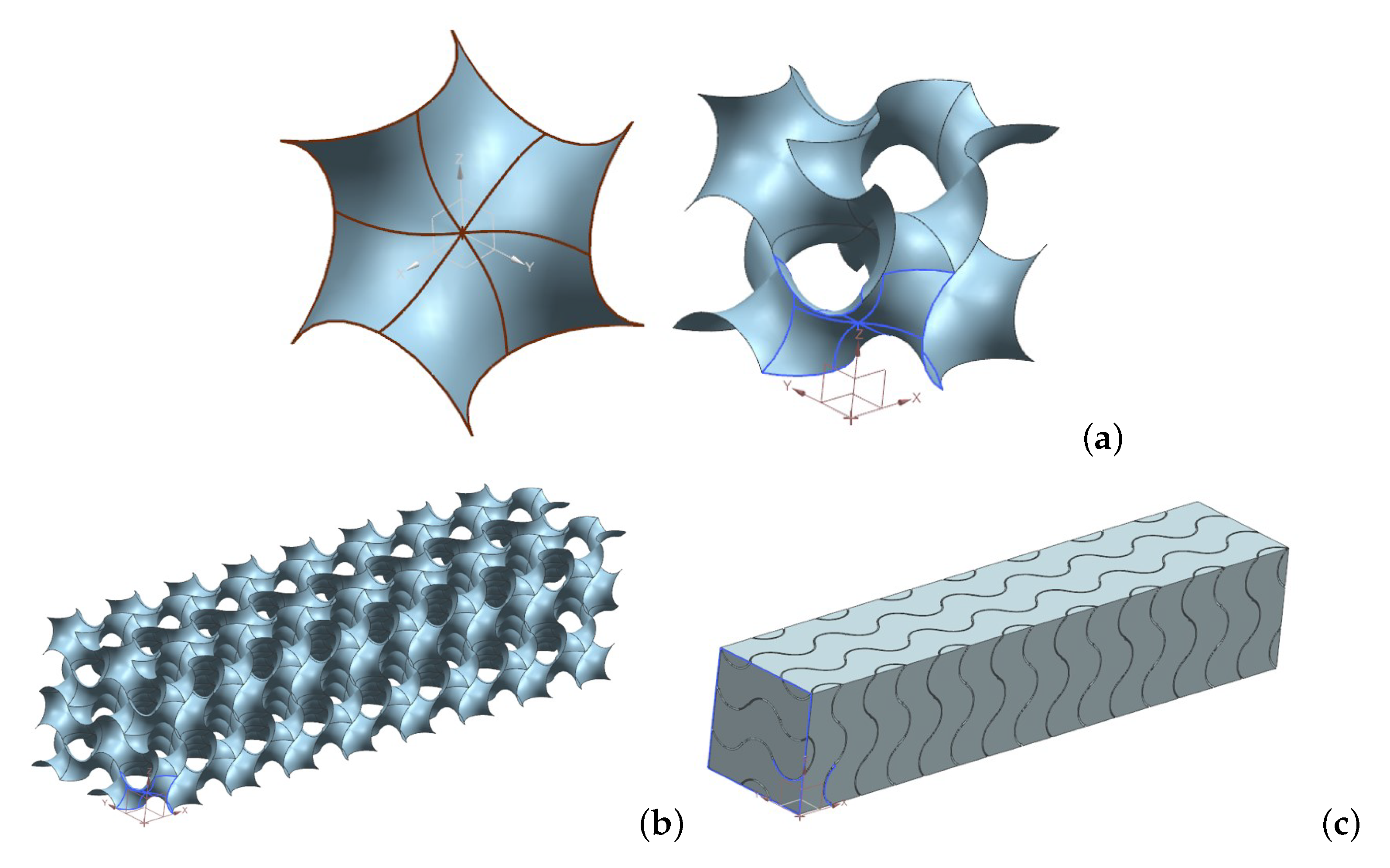A similarity between porous structures and some periodic structures such as triply periodic minimal surfaces (TPMS) has been recently suggested in the literature [28]. These structures have a potential application in the field of metal foam heat exchangers also because they can be obtained by additive manufacturing 3D printing techniques. For these reasons, in this work a metal foam with a periodic structure has been considered. The porous structure has been built starting from a surface called gyroid, shown in Figure 2, that is a combination of trigonometric functions such as:

$$\begin{array}{c}f=sin\left(\frac{2\pi x}{a}\right)cos\left(\frac{2\pi y}{a}\right)+sin\left(\frac{2\pi y}{a}\right)cos\left(\frac{2\pi z}{a}\right)+sin\left(\frac{2\pi z}{a}\right)cos\left(\frac{2\pi x}{a}\right),\end{array}$$

(27)

where a is the spatial periodicity of the function.

The fluid volume has been created starting from a fundamental surface unit shown in Figure 3a, left. This unit has been copied and rotated by means of a computer aided design software (Siemens Nx) to obtain the periodic surface, as shown in Figure 3a, right. Then, the periodic structure has been copied and translated to build the representative elementary volume employed for the volume-averaging of the physical fields (velocity, pressure, temperature). Such a representative elementary volume has a square section with dimensions $H=W=0.01$ m and a length $L=0.05$ m. The surface of the gyroid structure has been thickened to create a solid geometry representing the metal foam shown in Figure 3b. The computational domain has been finally obtained by subtracting to the geometry of the representative elementary volume the metal foam volume (as shown in Figure 3c).

The computational domain has been discretized to obtain an unstructured mesh with $5.545696\times {10}^6$ elements by means of StarCCM+ $2019.2$ software. The left surface in Figure 3c is the inlet section of the flow, while the surfaces perpendicular to the inlet section has been set as symmetry planes. In the outlet section, perpendicular to the x axis, a Neumann condition for the velocity and temperature, and a zero pressure condition are prescribed. The Navier-Stokes equations have been solved numerically for the laminar flow of water within the pores, together with the forced convection Fourier equation:

$$\begin{array}{c}\rho u_j\frac{\partial u_i}{\partial x_j}=-\frac{\partial p}{\partial x_j}+\mu {\nabla }^2{u}_i,\end{array}$$

(28)

and

$$\begin{array}{c}{u}_j\frac{\partial T}{\partial x_j}=\alpha {\nabla }^{2}T,\end{array}$$

(29)

where $u_i$ are the components of the velocity field, T is the fluid temperature, $\rho$, $\mu$ and $\alpha$ are respectively the density, dynamic viscosity and thermal diffusivity of the fluid. Six uniform velocities have been considered as inlet conditions ($u=$ 0.001 m/s ÷ 0.006 m/s), each with three different fixed and uniform solid structure temperatures ($T_s=25$ °C, $T_s=50$ °C, $T_s=75$ °C), while the inlet temperature of the flow has been set equal to 20 °C for each case. The Reynolds number ranges from 3.6 to 21.6, if the characteristic length is the spatial periodicity of the metal foam, $a=0.003$ m.

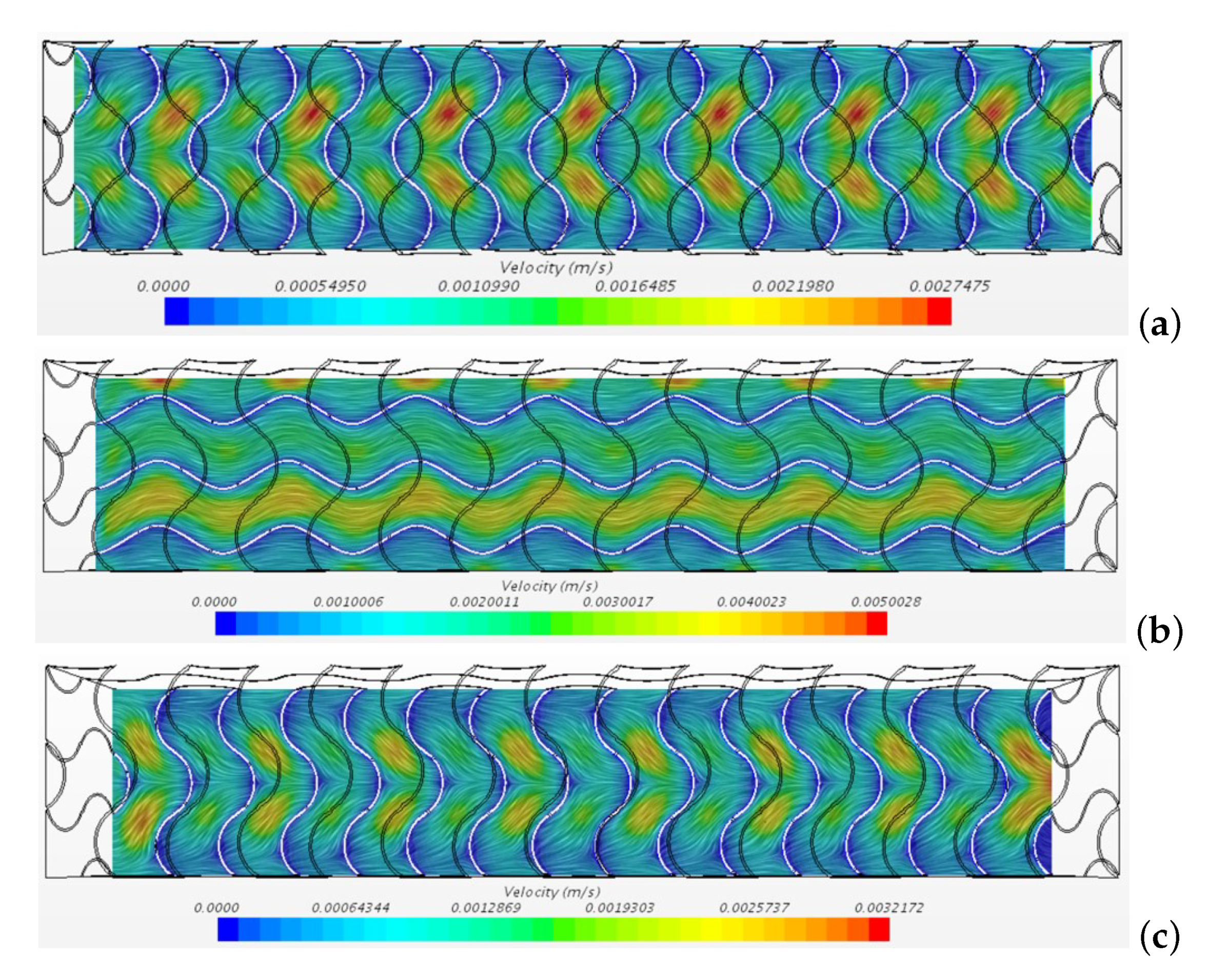
6.1. CFD Results—Velocity Field

The cases considered represent a simultaneously-developing laminar flow. Figure 4 shows the streamlines obtained for the case $\mathrm{Re}=3.6$, coloured with the velocity magnitude. This case corresponds to a inlet velocity $v=0.001$ m/s.

The figure shows winding paths within the pores, with a maximum velocity around $v_{max}=0.006$ m/s, i.e., six times the inlet velocity. Figure 5 shows the streamlines obtained for the same case on three planes at $y/H=1/3$, $y/H=1/2$ and $y/H=2/3$.

The planes $y/H=1/3$ and $y/H=2/3$ cut the inner pores of the metal foam in the middle, while the plane $y/H=1/2$ cuts the computational domain in the middle. The streamlines in the planes $y/H=1/3$ and $y/H=2/3$ evidence respectively separating and merging fluxes while wiggling in the direction z, as shown by Figure 6. The Figure 5 and Figure 6 evidence the symmetry of the velocity field under the exchange between the y and z coordinates.

Similar results are obtained for the cases with higher Re numbers, with a non-uniform velocity distribution that shows higher peaks as velocity increases, even in the developed flow region. Figure 7 shows the velocity peaks obtained on different sections along the x direction for the case $\mathrm{Re}=21.6$. This figure shows that the flow can be considered fully developed for $x/L>4/7$.

The pressure distribution is non-uniform as well. Figure 8 shows the pressure obtained for the case $\mathrm{Re}=3.6$ on the planes $y/H=1/3$, $y/H=1/2$ and $y/H=2/3$.

By plotting the pressure gradient as a function of the inlet velocity one obtains Figure 9.

Figure 9 shows that the trend is not linear. By fitting the data with the following function

$$\begin{array}{c}\left|\frac{\partial p}{\partial x}\right|=\frac{\mu }{K}u+\beta \rho u^2,\end{array}$$

(30)

where K is the permeability and $\beta$ is the Forchheimer coefficient one obtains

$$\begin{array}{c}\frac{\mu }{K}=5.54\times {10}^4\to K=1.60\times {10}^{-8} {\mathrm{m}}^2,\end{array}$$

(31)

and

$$\begin{array}{c}\beta \rho =5.03\times {10}^6\to \beta =5.03\times {10}^3 {\mathrm{m}}^{-1}.\end{array}$$

(32)

By using the permeability and the Forchheimer coefficient obtained from Equations (31) and (32) one obtains the following form drag coefficient

$$\begin{array}{c}{C}_F=\beta \sqrt{K}=0.67.\end{array}$$

(33)

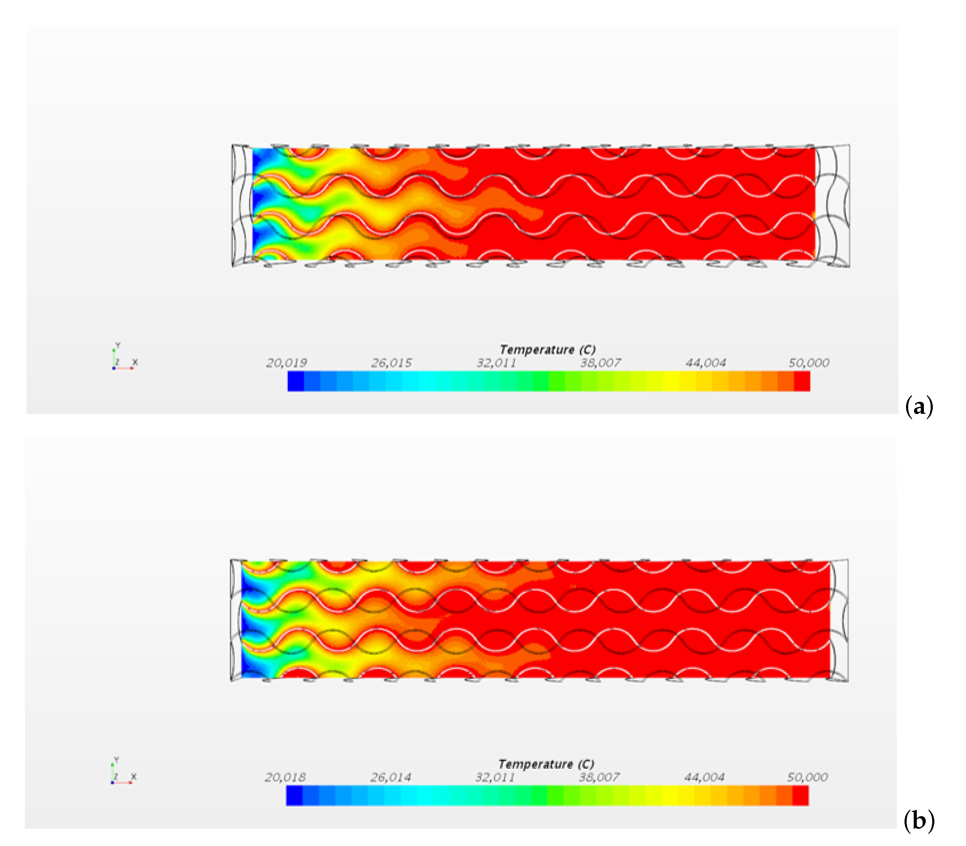
6.2. CFD Results—Temperature Field

The temperature distribution obtained reflects the velocity field shown in the previous section. Figure 10 shows the temperature distribution obtained on the planes $z/W=1/3$ and $z/W=2/3$ for the case $\mathrm{Re}=3.6$. The temperature on the structure surface is $T_s=50$ °C.

The figure shows that higher temperatures are reached where the velocity is lower. The computational data shows the observed mixing of the flow enhances the heat transfer within the metal foam. The temperature distribution on the plane $z/W=1/3$ is shown in Figure 11 for different inlet velocities and for a temperature on the porous structure $T_s=50$ °C.

The figure shows that the length of the thermally developing region increases with the velocity. However, the Nusselt number shows that the flow is thermally developed in the region with $x/L>6/7$ for all the cases. The interfacial heat transfer coefficient $h_I$ (W/(m² K)) obtained in the thermally developed region and the volumetric heat transfer coefficient h (W/(m³ K)) described in Equation (26) are reported in

Table 1. Heat transfer coefficients.

Inlet Velocity (m/s)	${\mathit{h}}_{\mathit{I}}$ (W/(m2 K))	h (W/(m3 K))
0.001	15.0	3.038 $\times {10}^4$
0.002	36.0	7.290 $\times {10}^4$
0.003	48.1	9.720 $\times {10}^4$
0.004	60.0	1.215 $\times {10}^5$
0.005	68.4	1.385 $\times {10}^5$
0.006	76.8	1.555 $\times {10}^5$

.

This result is in good agreement with the values reported in the literature for periodic structures such as Kelvin structure [29]. Figure 12 shows the comparison of the volumetric heat transfer coefficient h obtained in the present paper with the correlation obtained by Wu et al. for Kelvin structures [30]:

$$\begin{array}{c}h=\left(32.504{\epsilon }^{0.38}-109.94{\epsilon }^{1.38}+166.65{\epsilon }^{2.38}-86.98{\epsilon }^{3.38}\right){\mathrm{Re}}_{\mathrm{c}}^{0.438}{\epsilon }^{0.438}\frac{k_f}{d_c^2},\end{array}$$

(34)

where $d_c=a$ is the cell characteristic length [30], $k_f$ is the fluid thermal conductivity and $\epsilon =0.953$ is the porosity. In Equation (34), the Reynolds number has been evaluated with reference to the characteristic length $d_c$ [30].

These results show that periodic structures generated by a gyroid surface are characterised by heat transfer coefficients similar to those obtained for other periodic structures. The volumetric heat transfer coefficient obtained from local interface heat transfer coefficient gives a validation of the macroscopic averaged model, together with the LTNE assumption.

7. Conclusions

A survey of the volume-averaged models adopted to describe the momentum transfer and the heat transfer in a metal foam has been presented. The limiting case where the ratio between the thermal conductivity of the fluid and the thermal conductivity of the solid is much smaller than unity is described. With the aim of validating such volume-averaged models, CFD computation has been employed. Forced convection of water within a metal foam has been studied numerically by solving the Navier-Stokes and Fourier equations by means of a finite volume CFD code (StarCCM+ $2019.2$). The metal foam structure has been defined on the basis of the gyroid surface, a triply periodic minimal surface (TPMS), given by a combination of trigonometric functions. Under the simplifying assumption that the metal foam is a perfect heat conductor, a constant temperature boundary condition has been prescribed at the surface of the solid structure. Different inlet fluid velocities and solid surface temperatures have been assigned to characterise the fluid velocity distribution and the interphase heat transfer coefficient. A nonlinear correlation between the pressure gradient and the inlet velocity has been obtained, showing that the Darcy–Forchheimer model is a good approximation for the flow-through periodic porous structures. The volumetric interphase heat transfer coefficient has also been obtained, showing a good agreement with the literature. Generally speaking, the Darcy–Forchheimer model and the LTNE model adopted to describe the momentum and energy transfer in metal foams have been validated for metal periodic structures.

References

1. Boomsma, K.; Poulikakos, D.; Zwick, F. Metal foams as compact high performance heat exchangers. Mech. Mater. 2003, 35, 1161–1176. [Google Scholar] [CrossRef]
2. Krishnan, S.; Murthy, J.Y.; Garimella, S.V. Metal foams as passive thermal control systems. In Emerging Topics in Heat and Mass Transfer in Porous Media; Vadász, P., Ed.; Springer: Berlin/Heidelberg, Germany, 2008; pp. 261–282. [Google Scholar]
3. Mahjoob, S.; Vafai, K. A synthesis of fluid and thermal transport models for metal foam heat exchangers. Int. J. Heat Mass Transf. 2008, 51, 3701–3711. [Google Scholar] [CrossRef]
4. Zhao, C.Y. Review on thermal transport in high porosity cellular metal foams with open cells. Int. J. Heat Mass Transf. 2012, 55, 3618–3632. [Google Scholar] [CrossRef]
5. Ranut, P. On the effective thermal conductivity of aluminum metal foams: Review and improvement of the available empirical and analytical models. Appl. Therm. Eng. 2016, 101, 496–524. [Google Scholar] [CrossRef]
6. Nield, D.A.; Bejan, A. Convection in Porous Media, 5th ed.; Springer: Berlin/Heidelberg, Germany, 2017. [Google Scholar]
7. Kuznetsov, A.V. Thermal nonequilibrium forced convection in porous media. In Transport Phenomena in Porous Media; Ingham, D.B., Pop, I., Eds.; Pergamon: Oxford, UK, 1998; pp. 103–129. [Google Scholar]
8. Rees, D.A.S.; Pop, I. Local thermal non-equilibrium in porous medium convection. In Transport Phenomena in Porous Media III; Ingham, D.B., Pop, I., Eds.; Pergamon: Oxford, UK, 2005; pp. 147–173. [Google Scholar]
9. Vadasz, P. Explicit conditions for local thermal equilibrium in porous media heat conduction. Transp. Porous Media 2005, 59, 341–355. [Google Scholar] [CrossRef]
10. Vadasz, P. Lack of oscillations in dual-phase-lagging heat conduction for a porous slab subject to imposed heat flux and temperature. Int. J. Heat Mass Transf. 2005, 48, 2822–2828. [Google Scholar] [CrossRef]
11. Vadasz, P. Absence of oscillations and resonance in porous media dual-phase-lagging Fourier heat conduction. J. Heat Transf. 2005, 127, 307–314. [Google Scholar] [CrossRef]
12. Vadasz, P. On the paradox of heat conduction in porous media subject to lack of local thermal equilibrium. Int. J. Heat Mass Transf. 2007, 50, 4131–4140. [Google Scholar] [CrossRef]
13. Wang, L.; Xu, M.; Wei, X. Dual-phase-lagging and porous-medium heat conduction processes. In Emerging Topics in Heat and Mass Transfer in Porous Media; Vadász, P., Ed.; Springer: Berlin/Heidelberg, Germany, 2008; pp. 1–37. [Google Scholar]
14. Vadasz, P. Small Nield number convection in a porous layer heated from below via a constant heat flux and subject to lack of local thermal equilibrium. J. Porous Media 2012, 15, 249–258. [Google Scholar] [CrossRef]
15. Straughan, B. Convection with Local Thermal Non-Equilibrium and Microfluidic Effects; Springer: Berlin/Heidelberg, Germany, 2015. [Google Scholar]
16. Banu, N.; Rees, D.A.S. Onset of Darcy-Bénard convection using a thermal non-equilibrium model. Int. J. Heat Mass Transf. 2002, 45, 2221–2228. [Google Scholar] [CrossRef]
17. Barletta, A.; Rees, D.A.S. Local thermal non-equilibrium effects in the Darcy-Bénard instability with isoflux boundary conditions. Int. J. Heat Mass Transf. 2012, 55, 384–394. [Google Scholar] [CrossRef] [Green Version]
18. Rees, D.A.S. Microscopic modelling of the two-temperature model for conduction in heterogeneous media: Three-dimensional media. In Proceedings of the 4th International Conference on Application of Porous Media, Istanbul, Turkey, 10–12 August 2009. [Google Scholar]
19. Rees, D.A.S. Microscopic modeling of the two-temperature model for conduction in heterogeneous media. J. Porous Media 2010, 13, 125–143. [Google Scholar] [CrossRef]
20. Jamalud-Din, S.D.; Rees, D.A.S.; Reddy, B.V.K.; Narasimhan, A. Prediction of natural convection flow using network model and numerical simulations inside enclosure with distributed solid blocks. Heat Mass Transf. 2010, 46, 333–343. [Google Scholar] [CrossRef]
21. Dixit, T.; Ghosh, I. An experimental study on open cell metal foam as extended heat transfer surface. Exp. Therm. Fluid Sci. 2016, 77, 28–37. [Google Scholar] [CrossRef]
22. Cancellara, S.; Greppi, M.; Dongellini, M.; Fabbri, G.; Biserni, C.; Morini, G.L. Experimental investigation on the pressure drop of air flows through aluminum and nickel-chromium metallic foams for HVAC applications. Energies 2019, 13, 172. [Google Scholar] [CrossRef] [Green Version]
23. Alazmi, B.; Vafai, K. Constant wall heat flux boundary conditions in porous media under local thermal non-equilibrium conditions. Int. J. Heat Mass Transf. 2002, 45, 3071–3087. [Google Scholar] [CrossRef]
24. Yang, K.; Vafai, K. Analysis of temperature gradient bifurcation in porous media—An exact solution. Int. J. Heat Mass Transf. 2010, 53, 4316–4325. [Google Scholar] [CrossRef]
25. Nield, D.A. A note on local thermal non-equilibrium in porous media near boundaries and interfaces. Transp. Porous Media 2012, 95, 581–584. [Google Scholar] [CrossRef]
26. Polyaev, V.M.; Mozhaev, A.P.; Galitseysky, B.M.; Lozhkin, A.L. A study of internal heat transfer in nonuniform porous structures. Exp. Therm. Fluid Sci. 1996, 12, 426–432. [Google Scholar] [CrossRef]
27. Ranut, P.; Nobile, E.; Mancini, L. High resolution microtomography-based CFD simulation of flow and heat transfer in aluminum metal foams. Appl. Therm. Eng. 2014, 69, 230–240. [Google Scholar] [CrossRef]
28. Maskery, I.; Sturm, L.; Aremu, A.O.; Panesar, A.; Williams, C.B.; Tuck, C.J.; Wildman, R.D.; Ashcroft, I.A.; Hague, R.J.M. Insights into the mechanical properties of several triply periodic minimal surface lattice structures made by polymer additive manufacturing. Polymer 2018, 152, 62–71. [Google Scholar] [CrossRef]
29. Iasiello, M.; Cunsolo, S.; Bianco, N.; Chiu, W.K.S.; Naso, V. Developing thermal flow in open-cell foams. Int. J. Therm. Sci. 2017, 111, 129–137. [Google Scholar] [CrossRef]
30. Wu, Z.; Caliot, C.; Flamant, G.; Wang, Z. Numerical simulation of convective heat transfer between air flow and ceramic foams to optimise volumetric solar air receiver performances. Int. J. Heat Mass Transf. 2011, 54, 1527–1537. [Google Scholar] [CrossRef]
Figure 1. Samples of aluminium (a) and copper (b) foams.
Fluids 05 00155 g001aFluids 05 00155 g001b
Figure 2. Structure of the gyroid.
Fluids 05 00155 g002
Figure 3. Creation of the gyroid from the unit surface (a) to the metal foam structure (b) and the fluid volume (c).
Fluids 05 00155 g003
Figure 4. Streamlines obtained for the case Re = 3.6 .
Fluids 05 00155 g004
Figure 5. Streamlines for the case Re = 3.6 on three planes y / H = 1 / 3 (a) y / H = 1 / 2 (b) and y / H = 2 / 3 (c).
Fluids 05 00155 g005
Figure 6. Streamlines for the case Re = 3.6 on three planes z / W = 1 / 3 (a) z / W = 1 / 2 (b) and z / W = 2 / 3 (c).
Fluids 05 00155 g006
Figure 7. Velocity distribution on different sections of the metal foam for the case Re = 21.6 . Sections x / L = 4 / 7 (a) x / L = 5 / 7 (b) and x / L = 6 / 7 (c).
Fluids 05 00155 g007
Figure 8. Pressure distribution for the case Re = 3.6 on three planes y / H = 1 / 3 (a) y / H = 1 / 2 (b) and y / H = 2 / 3 (c).
Fluids 05 00155 g008
Figure 9. Pressure gradient versus inlet velocity.
Fluids 05 00155 g009
Figure 10. Temperature distribution obtained for the case Re = 3.6 , T s = 50 °C on the planes z / W = 1 / 3 (a) and z / W = 2 / 3 (b).
Fluids 05 00155 g010
Figure 11. Temperature distribution obtained on the plane z / W = 1 / 3 for the cases Re = 3.6 (a), Re = 7.2 (b), Re = 10.8 (c), Re = 14.4 (d). For all the cases, T s = 50 °C.
Fluids 05 00155 g011
Figure 12. Comparison of the volumetric heat transfer coefficient obtained in the present paper with Wu et al. correlation [30].
Fluids 05 00155 g012