Abstract
The applicability of adjoint-based gradient computation is investigated in the context of interfacial flows. Emphasis is set on the approximation of the transport of a characteristic function in a potential flow by means of an algebraic volume-of-fluid method. A class of optimisation problems with tracking-type functionals is proposed. Continuous (differentiate-then-discretize) and discrete (discretize-then-differentiate) adjoint-based gradient computations are formulated and compared in a one-dimensional configuration, the latter being ultimately used to perform optimisation in two dimensions. The gradient is used in truncated Newton and steepest descent optimisers, and the algorithms are shown to recover optimal solutions. These validations raise a number of open questions, which are finally discussed with directions for future work.
1. Introduction
Two-phase flows are central to a wide range of environmental and technological applications [1,2,3,4]. Energy conversion systems, for example, often rely on the combustion of high-energy-density liquid fuels to meet weight and volume restrictions. The flows encountered in such systems are often turbulent, and therefore encompass a vast range of spatial and temporal scales. In addition to multiple scales, these flows contain multiple physical and chemical phenomena such as capillarity, combustion, flow separation, radiation, and pollutant formation. These phenomena are of different nature, and their intricate coupling makes their understanding and prediction particularly challenging. As a consequence of the remarkable advances in computational sciences realized over the past decades, complex physical processes can now be simulated with an astonishing degree of fidelity and accuracy. In the case of two-phase flows, in particular, simulation and modeling have evolved from simplistic or back-of-the-envelop estimates (integral balance, analytical analysis) to petascale and soon exascale computing applications, generating unprecedented amounts of information.
While simulations of complex flows with increasing degree of confidence is of great importance, the ability to extract relevant optimization and control strategies dedicated to improving their performance and efficiency is as crucial. Access to such optimization strategies would have vast implications in many areas such as coating, crop protection, inkjet printing, and energy conversion devices [5,6]. From an environmental perspective, taking the example of energy conversion devices, the existence of such capabilities will have a large impact on reducing pollutants/emissions (NOx, soot, etc.), from the oceans all the way to the atmosphere, leading to cleaner and more efficient sources of energy.
Optimisation techniques materialize this shift in two ways: (i) Gradient-based methods and (ii) derivative-free techniques. Examples of derivative-free algorithms include pattern search methods, approximation models, response surfaces and evolutionary/heuristic global algorithms. While an efficient class of generic algorithms based on the surrogate management framework [7] and artificial neural networks [8] have been used for optimization in fluid mechanics, mainly in the area of aerodynamic shape optimization, they could require many function evaluations, for training purposes, for example. When detailed simulations of interfacial flows are concerned, each function evaluation commands a full (commonly unsteady) CFD computation. In such situations, gradient-based methods are at an advantage.
Common methods in extracting the gradient information are analytical or use finite differences. As far as the analytical determination of the gradient is concerned, the subtleties associated with the numerical approach, such as the meshing process, discretization, and the complexity of the governing equations, especially when regions with steep gradients or discontinuities (interfaces) are present, make extracting the analytical gradient expression close to impossible, and hence suffers from limited applicability. In the case of finite differences, the numerous parameters involved in modeling make this approach prohibitively expensive for large problems and can also be easily overwhelmed by numerical noise. Adjoint-based methodology allows determining the gradient at a cost comparable to a single function evaluation, regardless of the number of parameters, and is therefore a suitable alternative. Using this approach, gradient is computed in the form of algebraic or differential equations based on the problem’s Lagrange multipliers or adjoint variables, which in turn is used in standard optimization algorithms that rely on Jacobian information (such as the conjugate-gradient family). The use of adjoint methods for design and optimization has been an active area of research, which started with the pioneering work of Pironneau [9] with applications in fluid mechanics and later in aeronautical shape optimization by Jameson and co-workers [10,11,12]. Ever since these groundbreaking studies, adjoint-based methods have been widely used in fluid mechanics, especially in the fields of acoustics and thermo-acoustics [13,14]. These areas provide a suitable application for adjoint-based methods, which are inherently linear, since they too are dominated by linear dynamics. Recently, nonlinear problems have also been tackled, within the context of optimal control of separation on a realistic high-lift airfoil or wing, enhancement of mixing efficiency, minimal turbulence seeds and shape optimization to name a few [15,16,17,18]. The presence of discontinuities due to interfaces, together with the unsteady nature of relevant multiphase flow configurations constitutes another step in complexity.
As far as interfacial flows are concerned, significant research efforts have been dedicated to sensitivity analysis of thermal-hydraulic models for light-water reactor simulations, led by Cacuci [19,20]. The formalism developed by Cacuci and co-workers is based upon the two-fluid methodology, which requires a large number of closure assumptions (especially related to the interface topology) and lacks predictability in the absence of experimental data. A second research effort can be found in the motion planning of crystal growth and molten metal solidification, where by adjusting heat deposition on a sample, one controls the geometry of the solid-liquid interface [21,22]. Transport phenomena in solidification are limited to heat diffusion. While interface motion due to energy balance raises a significant number of challenges (Stefan flow), convective, viscous and capillary effects are absent. The underlying mathematical challenges, even in the low-Reynolds and Weber number ranges, remain widely unexplored. Likewise, adjoint-based methods have also been applied for optimization purposes in multi-phase flows through porous media (Darcy flow [23]). Since the adjoint-based methods in the context of multiphase models have, to date, not been applied to high-fidelity simulation of unsteady interfacial flows, it remains an open question that needs addressing.
The proposed study, therefore, focuses on the control of an interface in a potential flow for unity density and viscosity ratios in the absence of surface tension. The emphasis is set on (i) the solution of the characteristic function equation using an algebraic Volume-of-Fluid method (as opposed to the level set method in all documented studies) and (ii) the formulation of both continuous and discrete adjoint problems.
The manuscript is structured as follows: Section 2 describes the optimisation problem and the equations governing the evolution of the flow (primal problem), as well as the continuous adjoint equations (dual problem). Section 3 presents the discretization of the aforementioned problem (functional, primal and dual problems). The use of the adjoint-based gradient computation is implemented in a steepest descent framework in Section 4, ultimately applied in Section 5 where the results of one-dimensional and two-dimensional optimisations are presented and discussed. Finally, conclusions and perspective of this work are proposed in Section 6.
2. Continuous Governing Equations
Traditionally, adjoint equations are derived from the continuous primal (forward) equations by means of the Lagrange multiplier theory, and are used to obtain first-order sensitivity information for chosen cost functionals. Note that the resulting adjoint operators are then implemented using the differentiate-then-discretize approach, otherwise referred to as the continuous adjoint method. In this work, however, an alternative approach of discretize-then-differentiate is selected, where the spatially discretised primal equations are numerically processed and differentiated, to produce the associated adjoint code (discrete adjoint method). The continuous form of the adjoint equations, however, remains important since it clarifies the overall structure of the problem, and in particular how the gradient is computed updated throughout the iterative optimiser. Therefore, in this section, the equations governing the primal (direct/forward) and the dual (adjoint/backward) problems together with a consistent set of boundary conditions are presented. The discrete adjoint approach, used to generate the results of Section 5, will be presented subsequently in Section 3.
The problem of interest involves controlling the movement of the interface by means of boundary conditions on an auxiliary velocity field. In the general case, the evolution of the velocity field is governed by the incompressible Navier-Stokes equations. For the current application, a simplified potential flow is considered, where the inflow/outflow velocity on chosen boundaries is used as a control variable. In generic terms, the optimization problem may be summarized as follows
where the objective functional , the convex set of admissible control variables and the flow’s governing equations are described in the remainder of this section, together with the adjoint-based gradient computation.
2.1. Objective Functional
The objective function is constructed using tracking-type functionals of the following form
where,
and is a distance function whose zero level set matches the desired interface location, h denotes the controller, and the phase indicator. In order to express the norms appearing in the above equation, volume and surface inner products are defined, respectively, as follows,
with induced norms . This form of the objective functional is close to the one proposed by Bernauer et al. in the context of Stefan flow [22]. The first term on the right-hand side of Equation (2) matches the evolution of the interface, the second the value at the final time and the third is a regularization term for the control variable.
2.2. Primal (Forward) Problem
The two-phase Navier-Stokes equations, supplemented by a scalar advection equation characterizing the interface location (the characteristic function equation), form the so-called one-fluid formulation [24]. Following this approach, the evolution of interface is defined by the linear advection equation of an indicator (Heaviside) function
where is the velocity field, is the initial condition and denotes the Dirichlet boundary conditions prescribed on the inflowing boundary . The domain can be separated into two subdomains occupied by light () and dark () fluids, shown in Figure 1, such that
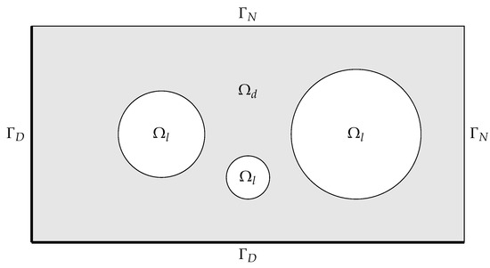
Figure 1.
Example geometry and boundary layout.
The velocity field driving the interface advection is assumed to be irrotational and incompressible. Therefore, there exists a velocity potential such that . The velocity potential must satisfy the following Laplace equation
where and are disjoint subsets of the domain boundary , over which, Dirichlet and Neumann boundary conditions are prescribed, respectively. The Neumann boundary conditions are used as the control quantity, whereas the Dirichlet boundary conditions are given and fixed. The case of is also considered, where all the domain boundaries are controlled.
The constraint set for the Neumann boundary conditions on the velocity potential is assumed to be a given Hilbert space. If , h must also satisfy the necessary condition for the existence of a solution to Equation (7)
The above constraint is also convex, so the resulting set will also be convex. Additional assumptions for the existence of a solution to the optimization problem (1) are given, e.g., in Gunzburger [25]. Uniqueness is out of scope for the current work, but can be expected, since all the equations and constraints in question are linear.
2.3. Dual (Adjoint) Problem
The theory of Lagrange multipliers is employed, to derive the continuous adjoint equations, and an augmented cost functional (Lagrangian) is constructed, with the constraints provided by Equations (5) and (7). For the optimization problem (Equation (1)), the Lagrangian is given by
where and are the associated Lagrange multipliers/adjoint variables. In order to compute the gradient of (required by the gradient-based optimizer used in this work), the variations with respect to all variables but h are set to zero.
By construction, the primal problem (Equations (5) and (7), which also include the initial and boundary conditions) is recovered by setting the variations with respect to the adjoint variables to zero. By setting the variations with respect to and to zero, the adjoint equations are obtained: Firstly, the advection equation for the adjoint volume fraction
where the source term comes from the derivative of the cost functional and is given by
with S as defined in Equation (3). It should be noted that the boundary conditions are only defined on the outflow boundaries of the adjoint equations. Since the adjoint is solved backward in time, boundaries outflowing in the primal problem turn into inflowing boundaries in the dual one.
Secondly, the adjoint velocity potential satisfies a Poisson equation
We can see that the boundary conditions on the adjoint velocity potential automatically satisfy the condition for the existence and uniqueness of a solution when . In addition, unless the interface intersects with the boundary of the computational domain, the Neumann boundary condition on the adjoint velocity potential will be homogeneous.
The variation with respect to the only remaining variable, h, yields the gradient, and is obtained by repeatedly applying integration by parts and matching terms when appropriate, resulting in
This gradient will ultimately be used in the gradient-based iterative algorithm, and will ultimately vanish once an extremum is reached. This is often referred to as the optimality condition.
3. Discrete Governing Equations
In this section, the discretisations of the primal and dual problems are presented. The main difference between the equations presented in Section 2 and those in this section is that the variables in the previous sections belong to an infinite dimensional functional Hilbert space, whereas in this section, the variables belong to a subspace of . As mentioned previously, the discretize-then-differentiate approach described here is the one that was ultimately used to produce the results in Section 5.
3.1. Objective Functional
The discrete form of the cost functional (2) is defined as
where N denotes the total number of timesteps. The required inner products are then constructed as follows,
where and denote the “volume” of cells and the “area” of cell faces intersecting the boundary, respectively (these definitions depends on the dimensionality of the problem). As such, we find that and are positive-definite diagonal weight matrices, allowing the definition of a non-degenerate associated norm.
3.2. The Thinc Scheme
For the discretization of the advection Equation (5) a variant of the algebraic Volume-of-Fluid (VOF) method, referred to as the THINC scheme [26], is used. The main advantages of algebraic Volume-of-Fluid methods, as opposed to geometric VOF, are their simplicity and their differentiability, a requirement in the context of gradient-based optimization.
Here the one-dimensional version of the THINC scheme presented in Xiao et al. [26] is briefly described. Standard finite volume notations are used, where is a cell of length centered at . This cell is bounded by two points that form the boundary . The discrete dependent field consists of the cell-averaged indicator function values also referred to as the volume fractions
For divergence-free velocity fields, Equation (5) may be recast in conservative form. Upon integrating over a cell , the semi-discrete equation is obtained
Finally, integration between and yields
where is as defined in Equation (17) and represents the flux through the face between and .
While classical finite volume methods leverage polynomial approximations of the dependent field to approximate the flux functions, the THINC scheme relies on a parametrization more suited to indicator functions, which over any given cell reads
or in non-dimensional form,
where
The global parameter , and the local ones are determined as follows:
- is the non-dimensional slope steepness, defining the sharpness of the interface. Larger values imply sharper interfaces. Note that is often expressed in terms of two other parameters as followswhere represents the number of cells for the hyperbolic tangent to transition from to ,
- is the interface directionwhere sgn denotes the signum function,
- is the non-dimensional intercept or jump location, which defines the level set of , and is imposed by the volume conservation constraintwhich can be inverted explicitly to givewhere .
The THINC approximation of the flux then consists of
where
and
Away from interfaces ( or ), the intercept value (Equation (25)) grows unbounded, which can trigger numerical instability. The THINC flux value itself however remains bounded, and the issue can be resolved by simply switching to the first order approximation presented below away from the interface.
On the one hand, it can be shown that
as and
as . On the other hand,
as and
as .
Given these first order approximations of the THINC flux away from interfaces, one simply needs to revert to the appropriate limit whenever or to construct a numerically stable flux.
3.3. Primal (Forward) Problem
Following spatial and temporal integration, the advection equation (Equation (5)) is discretized as follows
where, the discrete operator can be further broken into terms pertaining to each dimension, e.g., for two dimensions
This notation generalizes the one used in the previous section (Equation (18)) by defining more general operators, for example in the x direction
where, the numerical flux can be chosen as the THINC flux described in the previous section or any other (first order upwind, etc.). The operators in the other spatial directions are defined similarly. It should be noted that with this generalization no assumption is made as far as the compressibility of the velocity field is concerned. This condition will be satisfied through the velocity potential and its accuracy depends entirely on the accuracy of the Poisson solver and the approximation used.
Away from the boundaries, the discrete Laplace equation in two dimensions simply takes the following form,
with classical treatments of the Dirichlet and Neumann boundary conditions used where appropriate. Overall, the system of equations can be rewritten as
where is the vector of boundary conditions, defined as a function of the control variable . As in the continuous case, if , the Laplace operator is singular (with a null-space of dimension one spanned by the constant vector, noted ), so the right-hand side must satisfy
3.4. Dual (Adjoint) Problem
The Lagrangian of the discrete problem can be assembled, and the calculus of variations performed to ultimately derive the equation for the adjoint of the advection equation
where, denotes a pointwise evaluation of the function R defined in Equation (11). The final condition (the adjoint equation is marched backward in time) is
The adjoint velocity potential equation then becomes,
Finally, the gradient can now be obtained by differentiating with respect to , which yields
4. Optimisation Algorithm
In this work, a simple steepest decent algorithm is used to iteratively update the controler until the optimality condition is satisfied. More sophisticated algorithm (e.g., preconditioned nonlinear conjugate gradient method or Quasi-Newton methods such as the BFGS algorithm) can equally be used. The algorithm describing each step of the optimisation procedure is given in Algorithm 1.
| Algorithm 1: Optimization algorithm for Equation (1) |

|
5. Results
In this section, the results of the discrete adjoint methodology applied to one- and two-dimensional flow configurations are presented and described. The one-dimensional configuration is included for validation purposes. Once validated, the optimisation is performed in a two-dimensional setting and appropriate control strategies are extracted.
5.1. Validation: One-Dimensional Droplets
In the one-dimensional setting, the divergence-free condition imposes a constant velocity field, that matches the control variable (renamed c in the rest of this section). Therefore, the optimisation problem can be simplified accordingly, with the new cost functional reading
As mentioned, the use of velocity potential and the optimization of boundary conditions is not required, and hence not included. The remainder of the one-dimensional system is as described previously. The gradient is therefore given as,
and in discrete form,
This completes the definition of the optimization problem. The THINC flux approximation is then used to obtain , for all m and i. Using the computed volume fraction, the adjoint equations are solved and, finally the above cost function and gradient are computed. A truncated Newton algorithm (implemented in the numpy suite) is used in lieu of the steepest descent algorithm described in Section 4.
The desired interface will be given by the following signed distance function (analytical expression):
where is the velocity at which the desired interface moves. Additionally, , with final time , the desired velocity , and CFL condition is set at . The initial condition for the color function is given by mollifying the above signed distance function:
which can be seen in Figure 2. The parameters of the THINC scheme are and (which gives ). Finally, the initial guess for starting the iteration process of the optimization algorithm is , and weights .
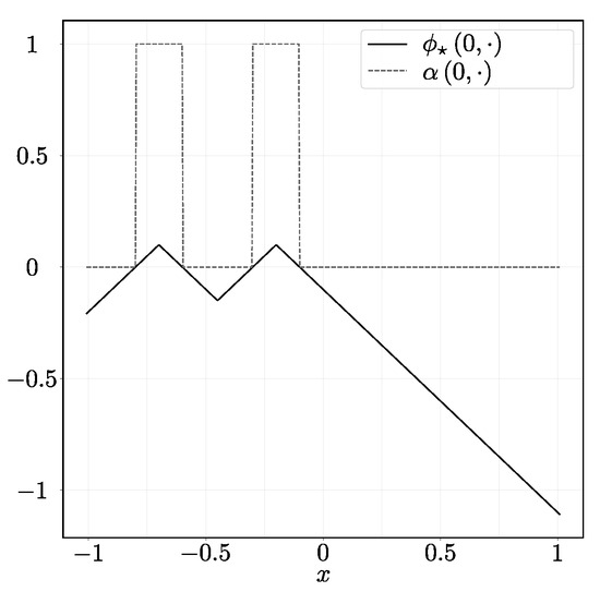
Figure 2.
Initial condition of the advection equation (dashed) and the signed distance function to the desired interface (solid).
The solution for and of the state and adjoint equations at time can be seen in Figure 3. As expected, for , the adjoint variable is uniformly zero, indicating an optimal solution. In the case , the adjoint equations computed by both continuous and discrete approaches are in good agreement. The adjoint variable assumes non-zero values only in the vicinity of the interface, indicating the direction in which the interface should evolve in order to reduce the objective functional.
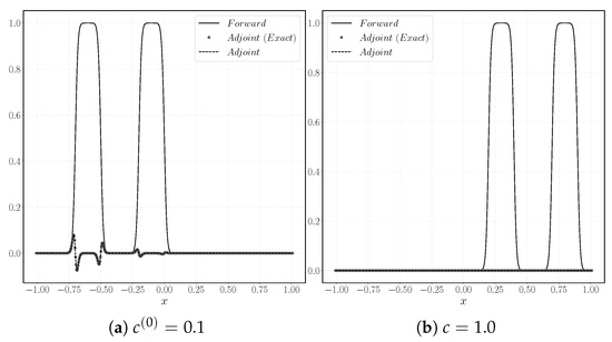
Figure 3.
Solution at time for the initial guess and the optimal solution .
The performances of the truncated Newton algorithm are displayed in Figure 4. Figure 4a shows that the value of the objective function decreases monotonically until the optimal value is reached at the sixth iteration. At this point, the value of cost function does not reduce any further. Note, that this value is not exactly zero: This is expected given the diffuse nature of the interface, and the average information used in definition of the tracking-type functional (Equation (14)). On the other hand, the residual (calculated by comparing to optimal c, Figure 4b) reaches zero machine also after six iterations as a consequence of the symmetry of the problem.
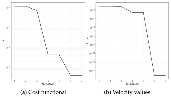
Figure 4.
Cost functional and velocity values at each function call in the optimization algorithm.
5.2. Two-Dimensional Tests
Having seen that the proposed optimization problem is well-posed and a correct optimal solution can be obtained in a one-dimensional setting, a two-dimensional configuration is considered. The spatial domain is set to and the focus is placed on the solution at the final time with the following weights:
A large weight () is attributed to the solution at time T, in order to ensure that the contribution of the adjoint variable dominates the calculated gradient. This has shown to improve the convergence speed of the steepest descent algorithm.
The desired interface contains a single droplet moving uniformly in the x direction. The signed distance function for such an interface is given by:
where is the droplet radius and
is the droplet center, moving with velocity . The desired velocity field has a uniform magnitude of 1, and the timestep is selected on the assumption that the velocity magnitude remains lower than 2 at all time, resulting in CFL condition set to .
The initial condition for the advection equation is given as,
The parameters for the mollifier are, a slope thickness of , and a cutoff value of , which give a slope steepness of .
The boundary conditions on the velocity potential are set as,
such that the left boundary of the domain is controlled with Neumann boundary conditions and all the remaining boundaries are uncontrolled with Dirichlet boundary conditions. The expected exact solution for the velocity potential is:
The Dirichlet boundary conditions can be computed from the above solution. The initial guess for the remaining Neumann boundary conditions, which are to be optimized, is given by a sinusoidal variation around the known optimal solution , resulting in
The initial distribution of the Neumann boundary condition, as well as, the location of the interface is shown in Figure 5. Figure 5a shows the initial location of the interface, shown by dashed lines. The initial guess for the Neumann boundary condition can also be seen in Figure 5b, defined on the left vertical boundary of the domain. The droplet is expected to travel left to right from the initial location (dashed lines in the figure). Due to the distribution of the velocity at the left boundary (sinusoidal wave), the velocity at the mid-domain is higher than the bottom and top, resulting in a squeezed droplet, identified by contours of volume fraction in Figure 5a. Of course, the resulting interface is different from the desired interface, identified by the solid line in the figure, and hence the need for an optimization procedure. Note, that the figure shows the initial and the end location of the particle, but the evolution of the interface at all times is considered in the objective function, defined by Equation (14).
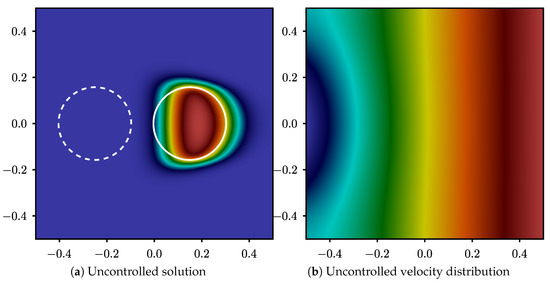
Figure 5.
Volume fraction and velocity potential of the uncontrolled solution: The dashed circle represents the initial location of the interface and the solid circle represents the desired interface location at .
As opposed to the one-dimensional problem, the linearization of the THINC flux (and therefore, its transpose Equation (40)) in the two-dimensional setting, gives rise to discontinuities away from the interface, where the interface direction changes sign. For one-dimensional advection, these changes typically occur at the center of a structure (droplet or bubble), and were mitigated by sharpening the interface sufficiently. In the two-dimensional setting, however, a similar strategy can not be devised: in regions where the interface is almost grid-aligned, the interface direction may change within a single cell, regardless of the steepness parameter. In this precise instance, the THINC scheme is not differentiable anymore. As a consequence, neither the gradient nor the adjoint equation are defined. In the case of a spherical structure, this occurs on the top, bottom, left and right of the droplet or bubble, and does not disappear by increasing the mesh resolution. Interestingly, this phenomenon does not occur in the direct vicinity of the interface, but away from it.
Alternative strategies were explored to alleviate this bottleneck, including the use of mollifier with compact support and the hybridisation with a first order upwind flux away from the interface [27]. However, none of the undertaken strategies proved to fully address the limitation of the THINC scheme, except for a differentiate-then-discretize approach, consisting of a THINC discretization (and a multidimensional extension such as THINC/SW [26]) for the direct problem, and the first order upwind flux for the linearization. This approach, however, while acceptable as far as contact discontinuities (including interfaces) are concerned, is shown to lead to divergent solutions in the presence of shocks [28]. Therefore, in this work, the discretize-then-differentiate principle of Section 5.1 is employed, together with a first order upwind scheme to approximate the volume fraction fluxes, instead of the THINC scheme used in the one dimensional example.
Figure 6 shows the volume fraction and the velocity field as produced after the extraction of the control strategy. Figure 6a shows that the volume fraction is now symmetric around the location of the desired interface (solid lines in the figure). On the other hand, this figure also demonstrates the limitation of the algorithm. Due to the use of a highly diffusive scheme (upwind) for convection of the interface, the volume fraction is diffused around the interface. Nevertheless, the distribution of the velocity potential in Figure 6b shows that the expected uniform velocity on the left vertical boundary is achieved through the control process. The uniform velocity allows the droplet to travel from left to the right of the domain without changing shape, conforming to the desired interface.
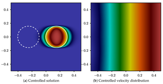
Figure 6.
Volume fraction and velocity potential of the controlled solution: The dashed circle represents the initial location of the interface and the solid circle represents the desired interface location at .
The performance of the optimization algorithm is presented in Figure 7. The evolution of the cost functional is reported for two terms: distributed part corresponding to (denoted by ), and final time part corresponding to (denoted by ). Based on the set values for ’s (Equation (49)), these two terms are the main contributors to the overall value of the cost functional. This figure shows that both terms are decreasing during the optimisation process. As expected with a steepest descent algorithm, progress is slow, but ultimately a minimum is reached. The minimum value is small but not zero. The origin of this discrepancy can be attributed to two main factors: (i) The interface is mollified, and only averaged characteristic values are used in the numerical functional (in this sense, numerical and desired interfaces will never identically match) and (ii) the upwind scheme is severely diffusive, which magnifies this effect. Both these factors can be seen in Figure 6 illustrating the distribution of the volume fraction, as mentioned before.
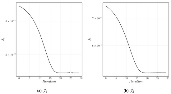
Figure 7.
Evolution of the two terms of the cost functional as a function of the descent iteration.
The adjoint variables themselves are also given in Figure 8. These figures show that the final state of the adjoint volume fraction is as expected zero around the zero level set of the desired interface and has a large error outside where the upwind scheme has diffused the solution. In the case of the adjoint velocity potential, similarly, the larger values can be found on the x axis, where the adjoint volume fraction has non-zero values. Adjoint variables can to some extent be used to analyze the gradient. One important hint that the gradient is correct is given by the adjoint velocity potential from Figure 8a. This figure shows that large negative values are present in the center of the left boundary of the domain. This is indeed the expected result since that is where the largest error in the initial guess of the control h resides, i.e., the top of the cosine bump. Towards the end, the value of the adjoint velocity potential becomes much more uniform on the left boundary, albeit not zero. The adjoint velocity potential can not become exactly zero on this boundary due to existing diffusion, reducing the overall accuracy of the result. Similar to the one-dimensional problem, good convergence is achieved, validating the previous analysis and formulation.
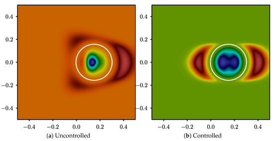
Figure 8.
Adjoint volume fraction: The solid circle represents the desired interface location.
6. Conclusions and Future Work
This study explored the feasability of control of interfaces in the context of algebraic volume-of-fluid methods. A potential flow where two fluids of equal densities and viscosities interact across an interface without surface tension is considered. A discretize-then-differentiate approach is applied to the THINC scheme and found to correctly predict the gradient of a tracking-type functional, which in turn is successfully minimized using a truncated Newton algorithm. As expected from the theory of hyperbolic systems, this one-dimensional application confirms that as contact discontinuities, interfaces can be controlled with readily available algebraic volume-of-fluid transport schemes. This is in contrast with genuinely non-linear waves (shocks), for which only temporally and spatially consistent adjoints with tailored numerical fluxes are known to yield converging adjoint solutions [28,29].
The linearization of the algebraic Volume-of-Fluid employed here, however, gives rise to singularities away from interfaces, where interface direction changes occur. In one-dimensional configurations, this lack of differentiability of the THINC scheme can be circumvented. This is not the case in dimensions two and higher. A first order upwind scheme is therefore chosen instead, and shown to effectively provide gradient information in a motion planning optimisation problem.
The aforementioned lack of differentiability raises the question of whether algebraic Volume-of-Fluid methods such as THINC are best suited for gradient computation. Along the same line, the binary information content of the volume fraction field (presence of the dark or light fluid) also raises challenges when it comes to formulating meaningful (and convex) tracking type functionals. This can allegedly be attributed to the simplicity of the potential flow model employed here, but prior to focusing future efforts on more physical models, the use of front-tracking techniques will be explored in future related work.
The addition of more physics will bring more relevant functionals along with more challenges, since they will also introduce topological changes. As a matter of fact, since phenomena such as ligament and sheet break-ups are not well-posed in the sharp interface limit (subcontinuum physics missing), the first step in this direction will explore the continuous and discrete adjoint formulations up until breakup/coalescence.
Finally, the optimiser itself, having a large impact on the rate of convergence, was found to be a critical part of the algorithm. Improvements including line search, preconditioning, and Newton-like methods will be evaluated against derivative-free methods.
Author Contributions
Conceptualization, A.F., V.L.C. and T.S.; methodology, A.F., V.L.C. and T.S.; software, A.F.; validation, A.F.; writing—original draft preparation, A.F., V.L.C. and T.S.; writing—review and editing, V.L.C. and T.S.; visualization, A.F.; supervision, V.L.C. and T.S. All authors have read and agreed to the published version of the manuscript.
Funding
Taraneh Sayadi kindly acknowledges financial support from Deutsche Forschungsgemeinschaft (DFG) through SFB/TRR 129.
Conflicts of Interest
The authors declare no conflict of interest.
References
- Mortazavi, M.; Le Chenadec, V.; Moin, P.; Mani, A. Direct numerical simulation of a turbulent hydraulic jump: Turbulence statistics and air entrainment. J. Fluid Mech. 2016, 797, 60–94. [Google Scholar] [CrossRef]
- Habla, F.; Fernandes, C.; Maier, M.; Densky, L.; Ferrás, L.L.; Rajkumar, A.; Carneiro, O.S.; Hinrichsen, O.; Nóbrega, J.M. Development and validation of a model for the temperature distribution in the extrusion calibration stage. Appl. Therm. Eng. 2016, 100, 538–552. [Google Scholar] [CrossRef]
- Fernandes, C.; Faroughi, S.A.; Carneiro, O.S.; Nóbrega, J.M.; McKinley, G.H. Fully-resolved simulations of particle-laden viscoelastic fluids using an immersed boundary method. J. Non Newton. Fluid Mech. 2019, 266, 80–94. [Google Scholar] [CrossRef]
- de Campos Galuppo, W.; Magalhães, A.; Ferrás, L.L.; Nóbrega, J.M.; Fernandes, C. New boundary conditions for simulating the filling stage of the injection molding process. Eng. Comput. 2020. [Google Scholar] [CrossRef]
- Khaliq, M.H.; Gomes, R.; Fernandes, C.; Nóbrega, J.M.; Carneiro, O.S.; Ferrás, L.L. On the use of high viscosity polymers in the fused filament fabrication process. Rapid Prototyp. J. 2017, 23, 727–735. [Google Scholar] [CrossRef]
- Le Chenadec, V.; Pitsch, H. A Conservative Framework For Primary Atomization Computation and Application to the Study of Nozzle and Density Ratio Effects. At. Sprays 2013, 23, 1139–1165. [Google Scholar] [CrossRef]
- Marsden, A.; Feinstein, J.; Taylor, C. A computational framework for derivative-free optimization of cardiovascular geometries. Comput. Methods Appl. Mech. Eng. 2008, 197, 1890–1905. [Google Scholar] [CrossRef]
- Pierret, S.; Coelho, R.; Kato, H. Multidisciplinary and multiple operating points shape optimization of three-dimensional compressor blades, Structural and Multidisciplinary Optimization. Comput. Methods Appl. Mech. Eng. 2007, 33, 61–70. [Google Scholar]
- Pironneau, O. On optimum design in fluid mechanics. J. Fluid Mech. 1974, 64, 97–110. [Google Scholar] [CrossRef]
- Jameson, A. Aerodynamic design via control theory. J. Sci. Comput. 1988, 3, 233–260. [Google Scholar] [CrossRef]
- Jameson, A.; Martinelli, L.; Pierce, N.A. Optimum Aerodynamic Design Using the Navier-Stokes Equations. Theor. Comp. Fluid Dyn. 1998, 10, 213–237. [Google Scholar] [CrossRef]
- Reuther, J.J.; Jameson, A.; Alonso, J.J.; Rimlinger, M.J.; Saunders, D. Constrained Multipoint Aerodynamic Shape Optimization Using an Adjoint Formulation and Parallel Computers, Part 2. J. Aircr. 1999, 36, 61–74. [Google Scholar] [CrossRef]
- Juniper, M. Triggering in the horizontal Rijke tube: Non-normality, transient growth and bypass transition. J. Fluid Mech. 2010, 667, 272–308. [Google Scholar] [CrossRef]
- Lemke, M.; Reiss, J.; Sesterhenn, J. Adjoint-based analysis of thermoacoustic coupling. AIP Conf. Proc. Am. Inst. Phys. 2013, 1558, 2163–2166. [Google Scholar]
- Nemili, A.; Özkaya, E.; Gauger, N.; Kramer, F.; Thiele, F. Discrete adjoint based optimal active control of separation on a realistic high-lift configuration. In New Results in Numerical and Experimental Fluid Mechanics X: Contributions to the 19th STAB/DGLR Symposium Munich, Germany, 2014; Springer: Berlin/Heidelberg, Germany, 2016; pp. 237–246. [Google Scholar]
- Schmidt, S.; Ilic, C.; Schulz, V.; Gauger, N. Three-dimensional large-scale aerodynamic shape optimization based on shape calculus. AIAA J. 2013, 51, 2615–2627. [Google Scholar] [CrossRef]
- Rabin, S.; Caulfield, C.; Kerswell, R. Designing a more nonlinearly stable laminar flow via boundary manipulation. J. Fluid Mech. R1 2014, 738, 1–12. [Google Scholar] [CrossRef]
- Foures, D.; Caulfield, C.; Schmid, P. Optimal mixing in two-dimensional plane Poiseuille flow at finite Péclet number. J. Fluid Mech. 2014, 748, 241–277. [Google Scholar] [CrossRef]
- Cacuci, D.G.; Ionescu-Bujor, M. Adjoint sensitivity analysis of the RELAP5 MOD3.2 two-fluid thermal-hydraulic code system—I: Theory. Nucl. Sci. Eng. 2000, 136, 59–84. [Google Scholar] [CrossRef]
- Ionescu-Bujor, M.; Cacuci, D.G. Adjoint sensitivity analysis of the RELAP5 MOD3.2 two-fluid thermal-hydraulic code system—II: Applications. Nucl. Sci. Eng. 2000, 136, 85–121. [Google Scholar] [CrossRef]
- Bernauer, M.K.; Herzog, R. Implementation of an X-FEM solver for the Classical two-phase Stefan problem. SIAM J. Sci. Comput. 2011, 52, 271–293. [Google Scholar] [CrossRef]
- Bernauer, M.K.; Herzog, R. Optimal control of the classical two-phase Stefan problem in level set formulation. SIAM J. Sci. Comput. 2011, 33, 342–363. [Google Scholar] [CrossRef]
- Bernauer, M.K.; Herzog, R. Adjoint-based optimization of multi-phase flow through porous media—A review. Comput. Fluids 2011, 46, 40–51. [Google Scholar]
- Kataoka, I. Local instant formulation of two-phase flow. Int. J. Multiph. Flow 1986, 12, 745–758. [Google Scholar] [CrossRef]
- Gunzburger, M.D. Perspectives in Flow Control and Optimization; Society for Industrial and Applied Mathematics: Philadelphia, PA, USA, 2003. [Google Scholar]
- Xiao, F.; Ii, S.; Chen, C. Revisit to the THINC Scheme: A Simple Algebraic VOF Algorithm. J. Comput. Phys. 2011, 230, 7086–7092. [Google Scholar] [CrossRef]
- Fikl, A. Adjoint-Based Optimization for Hyperbolic Balance Laws in the Presence of Discontinuities. Ph.D. Thesis, University of Illinois at Urbana-Champaign, Champaign, IL, USA, 2016. [Google Scholar]
- Fikl, A.; Le Chenadec, V.; Sayadi, T.; Schmid, P. A comprehensive study of adjoint-based optimization of non-linear systems with application to Burgers’ equation. In Proceedings of the 46th AIAA Fluid Dynamics Conference, Washington, DC, USA, 13–17 June 2016. [Google Scholar]
- Giles, M.B. Discrete Adjoint Approximations with Shocks. In Hyperbolic Problems: Theory, Numerics, Applications; Hou, T.Y., Tadmor, E., Eds.; Springer: Berlin/Heidelberg, Germany, 2003. [Google Scholar]


© 2020 by the authors. Licensee MDPI, Basel, Switzerland. This article is an open access article distributed under the terms and conditions of the Creative Commons Attribution (CC BY) license (http://creativecommons.org/licenses/by/4.0/).