Article

An Elastic Collision Model for Impulsive Jumping by Small Planktonic Organisms

Applied Ocean Physics & Engineering Department, Woods Hole Oceanographic Institution, Woods Hole, MA 02543, USA
Fluids 2020, 5(3), 154; https://doi.org/10.3390/fluids5030154
Submission received: 29 June 2020 / Revised: 2 September 2020 / Accepted: 4 September 2020 / Published: 5 September 2020
(This article belongs to the Special Issue Fluid Mechanics of Plankton)

Abstract

:
Many small marine planktonic organisms converge on similar propulsion mechanisms that involve impulsively generated viscous wake vortex rings, and small-scale fluid physics is key to mechanistically understanding the adaptive values of this important behavioral trait. Here, a theoretical fluid mechanics model is developed for plankton jumping, based on observations that the initial acceleration phase for a jumping plankter to attain its maximum speed is nearly impulsive, taking only a small fraction of the viscous timescale, and therefore can be regarded as nearly inviscid, analogous to a one-dimensional elastic collision. Flow circulation time-series data measured by particle image velocimetry (PIV) are input into the model and Froude propulsion efficiencies are calculated for several plankton species. Jumping by the tailed ciliate Pseudotontonia sp. has a high Froude propulsion efficiency ~0.9. Copepod jumping also has a very high efficiency, usually >0.95. Jumping by the squid Doryteuthis pealeii paralarvae has an efficiency of 0.44 ± 0.16 (SD). Jumping by the small medusa Sarsia tubulosa has an efficiency of 0.38 ± 0.26 (SD). Differences in the calculated efficiencies are attributed to the different ways by which these plankters impart momentum on the water during the initial acceleration phase as well as the accompanied different added mass coefficients.

Graphical Abstract

1. Introduction

Marine planktonic organisms play crucial roles in marine ecosystems and biogeochemical cycling in the world ocean; however, most of them are of microscopic size, having no or limited swimming capabilities relative to the macroscopic water parcels within which they are embedded. Although the water parcels themselves may constantly move in a turbulent, eddying way, the fluid environment at the spatial scales of individual plankters, generally less than a few millimeters, is a dominantly viscous world. Under oceanic turbulence conditions, a copepod is unlikely to face turbulent diffusion inside the spherical space of ~10 mm radius surrounding itself [1], while a small phytoplankton experiences only shear remnants of dissipative turbulent eddies across the space of ~1 mm diameter around itself [2]. Thus, within the fluid immediately surrounding a plankter, the low-Reynolds-number fluid dynamics together with small-scale diffusion governs the transport of mass and momentum, thereby shaping the energy, matter, and information flows to and from the plankter. The small-scale fluid physics is key to mechanistically understanding the adaptations that small marine planktonic organisms engage in to fulfill three main survival tasks, namely feeding, predator avoidance, and reproduction, in the three-dimensional viscous water environment [3,4,5,6,7]. The small-scale fluid physics interfaces with the morphology, behavior, perception, response, and interaction of these small organisms to produce a variety of fascinating phenomena, patterns, processes, and functions that are fundamentally important to marine life, population and ecosystem functioning, and evolution.
Small marine planktonic organisms are morphologically, physiologically, and genetically diverse; however, living in the viscous water environment that is governed by the same small-scale fluid physics has driven convergent evolution of some of their key behavioral traits. For example, the ubiquitous, photosynthetic, jumping ciliate Mesodinium rubrum is a species complex that consists of at least six genetically diversified clades [8,9,10]. Nevertheless, morphologically, they all possess an equatorially located propulsive ciliary belt that enables them to jump both energetically more efficiently and hydrodynamically more quietly [11]; kinematically, they jump at different speeds according to their temperature zones but at the same mean jumping distance of around six body lengths, which is just above the thickness of the nutrient diffusive boundary layer surrounding the cell, indicating the constraint imposed compellingly by the small-scale advection–diffusion physics of the cell’s immediately surrounding water [12].
An even more compelling example is that many small marine plankters converge on similar propulsion mechanisms that involve impulsively generated viscous vortex rings. Despite differences in body morphology and size and propulsion machinery, copepods, copepod nauplii, squid paralarvae, small jellyfish, ciliates with contractible tail-like appendages, and freshwater Daphnia species generate impulsive viscous vortex rings for fast jumping motions [13,14,15,16,17,18,19] or feeding currents [20]. The flow field of an impulsively generated viscous vortex ring can be mathematically described by an impulsive Stokeslet or an impulsive stresslet [13,14], which are spatially limited and temporally ephemeral, thereby effectively reducing the predation risk due to a flow-sensing predator. A jump-imposed flow typically consists of a vortex around the jumping body and a wake vortex, both of which are in a near mirror-image configuration [21], thereby further reducing the predation risk by confusing the real position of the jumping body. Moreover, a relocating jump by a copepod achieves an extremely high Froude propulsion efficiency (>0.9), as revealed by both computational fluid dynamics (CFD) simulations [21] and particle image velocimetry (PIV) measurements [17]. The Froude propulsion efficiency (or hydromechanical efficiency [22]) is defined as
η W useful W total = 0 τ T ( t ) U ( t ) d t W total
where, to reflect the highly unsteady nature of jumping, the useful mechanical work Wuseful is calculated as the time integral of the product of the instantaneous thrust T(t) and jumping velocity U(t) over the thrust duration τ, and Wtotal is the total mechanical work done for creating the jumping motion. Physically, Wuseful is the mechanical work that is done to overcome body drag and accelerate the body with added mass to the maximum jumping velocity Umax. Although the extremely high Froude propulsion efficiency for copepod jumping appears quite counter-intuitive with respect to the dominantly viscous water environment in which the copepod resides, it simply means that the part of the mechanical work done to generate the wake vortex is significantly smaller than Wuseful. It is however unknown how the Froude propulsion efficiency varies for jumping by other small plankters that differ in body morphology and size and propulsion machinery.
In the present study, a theoretical fluid mechanics model is developed to calculate the Froude propulsion efficiency for fast jumping by a small plankter. The theoretical model is based on the appropriate assumption that, although the decay phase post the generation of the viscous vortex ring in the wake by an impulsively applied thrust is a highly viscous process, the initial acceleration phase for the body to attain Umax is brief and nearly impulsive and therefore can be regarded as a nearly inviscid process. The theoretical model is used to examine the effects on the Froude propulsion efficiency due to such factors as jumping impulsiveness, added mass coefficient, and the different ways by which those small plankters impart momentum on the water during the initial acceleration phase. It is highlighted that, here, the convergent evolution manifests itself in the behavioral traits which those small plankters possess to exert thrust on water in an astonishingly quick and impulsive fashion.

2. The Elastic Collision Model

Here, an elastic collision model is proposed for calculating the Froude propulsion efficiency of impulsive jumping by a small plankter. The theoretical model is developed by dividing the whole jumping process into two phases: an initial acceleration phase, in which the body is self-propelled briefly or impulsively to attain Umax, and then a deceleration phase, in which the body decelerates under the action of fluid drag while simultaneously the wake vortex ring initially generated in the acceleration phase decays due to viscosity.
For the acceleration phase, the impulsiveness of jumping ensures that the thrust duration τ is shorter than the viscous timescale defined as L2/(4ν), where L is a characteristic length scale (e.g., the body length) and ν is seawater kinematic viscosity, and that the nondimensional jump number defined as
N jump = τ L 2 / ( 4 ν )
is much smaller than 1. In fact, measurements did show that Njump << 1 (see below). Formally, τ and L are used as the time and length scale to conduct a dimensional analysis of the vorticity equation D ω D t = ω u + ν 2 ω ; since Njump << 1 implies τ L 2 / ν 1 , the viscous diffusion term ν 2 ω 
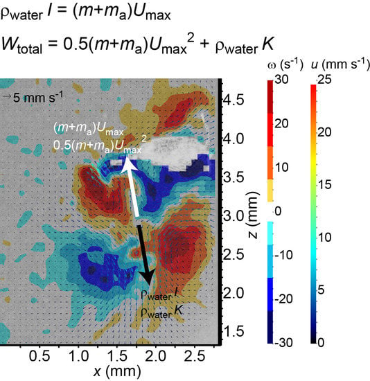
is negligible compared with the other two terms. Thus, the acceleration phase is approximately inviscid, and, except for the wake region, the flow around the accelerating body is approximately irrotational. This has two consequences: firstly, the skin drag can be neglected. Secondly, along with accelerating the body of mass m to Umax, the body’s surface pressure must increase to supply the force to accelerate the fluid around the body, i.e., the added mass ma must also be accelerated to Umax in order to set up the irrotational motion. Therefore, the total impulse of thrust must be (m + ma) Umax [23]. This can be analogous to a one-dimensional elastic collision: the total momentum (=0 at t = 0) is conserved in that the maximum momentum achieved by the accelerating body with added mass is equal in magnitude but opposite in direction to the impulse (ρwater × I) of the wake vortex ring that the body generates by impulsively exerting thrust on the water, i.e.,
ρ water   I = ( m + m a )   U max
where ρwater is seawater mass density and I is defined by Equations (A7), (A16), or (A26), respectively, for three types of wake vortex rings that are considered in the following. Moreover, the total mechanical energy that the body expends for propulsion is the addition of the maximum kinetic energy achieved by the accelerating body with added mass [ E 1 2 ( m + m a )   U max 2 ] and the kinetic energy (ρwater × K) of the wake vortex ring, where K is defined by Equations (A8), (A17), or (A27) for the considered three types of wake vortex rings, respectively. Here, the term “elastic collision” is borrowed to mean that the initial separation between the accelerating body and the wake vortex ring conserves both momentum and mechanical energy.
As m = ρbody Vbody and ma = α ρwater Vbody (where ρbody is body mass density, Vbody is body volume, and α is the added mass coefficient), substituting them into Equation (3) results in an expression for α:
α = I V body   U max ρ body ρ water
Moreover, from Equation (3), E can be rewritten as
E = ρ water 2   I 2 2 ( ρ body + α ρ water )   V body
Then, using E and K, the Froude propulsion efficiency can be calculated as
η E E + ρ water K
For the deceleration phase, the viscous timescale is now the timescale and therefore the viscous diffusion term ν 2 ω is no longer negligible; however, the physical properties of the viscously dissipating wake vortex ring can be used to work out a final formula for calculating the Froude propulsion efficiency. First, a nondimensional kinetic energy of the wake vortex ring is defined as
κ K I 1 / 2   Γ 3 / 2
where Γ is the circulation of the wake vortex ring. Second, substituting Equations (5) and (7) into Equation (6) and using Vbody = 4/3πR3 (where R is the equivalent spherical radius of the body) lead to
η = 1 1 + 8 π 3 κ   ( ρ body ρ water + α )   R 3   I 3 / 2   Γ 3 / 2
In Equation (8), I and Γ are informed by PIV measured flow data of the wake vortex ring, and α is calculated using Equation (4) from measured I and Umax.
In particular, if the wake vortex ring can be approximated by an impulsive Stokeslet (Appendix A), then it can be shown that
η iStokeslet = 1 1 + κ iStokeslet 3 π   ( ρ body ρ water + α )   ( R ν t * ) 3
where κ iStokeslet = 2 12 0.118 is the nondimensional kinetic energy of the impulsive Stokeslet, and t* = tmaxt0, where tmax is the time corresponding to the maximum circulation (Γmax) attained at the end of the acceleration phase (=at the beginning of the deceleration phase), and t0 is the virtual time origin that is determined by fitting the PIV measured time series of circulation for the deceleration (or decay) phase to the impulsive Stokeslet model (Equation (A6)).
Similarly, if the wake vortex ring can be approximated by one component of the viscous vortex ring pair described by an impulsive stresslet (Appendix B), then it can be shown that
η istresslet = 1 1 + κ istresslet 3 π   ( ρ body ρ water + α )   ( R ν t * ) 3
where κ istresslet = π 20 2 0.111 is the nondimensional kinetic energy of the impulsive stresslet, and t* = tmaxt0, where tmax is the time corresponding to the maximum circulation (Γmax) and t0 is the virtual time origin that is determined by fitting the time series of circulation for the decay phase to the impulsive stresslet model (Equation (A15)).
The nondimensional kinetic energy of the wake vortex ring, i.e., κ defined by Equation (7), is a key parameter to describe how energetically costly it is to impose a specific type of wake vortex ring. For a given impulse I and circulation Γ, the higher the value of κ, the higher the mechanical energy cost that is required to generate the specific wake vortex ring and therefore the lower the Froude propulsion efficiency. To illustrate this point, it is hypothetically assumed that a jumping plankter imposes a Hill’s spherical vortex (Appendix C) in the wake, and then the resulted Froude propulsion efficiency ηHill is compared with ηiStokeslet and ηistresslet. It can be shown that
η Hill = 1 1 + 10 10   κ Hill 3 π   ( ρ body ρ water + α )   ( R a ) 3
where κ Hill = 10 π 35 0.160 is the nondimensional kinetic energy of Hill’s spherical vortex, and a is the radius of the vortex. Note that κHill > κiStokeslet, κistresslet.
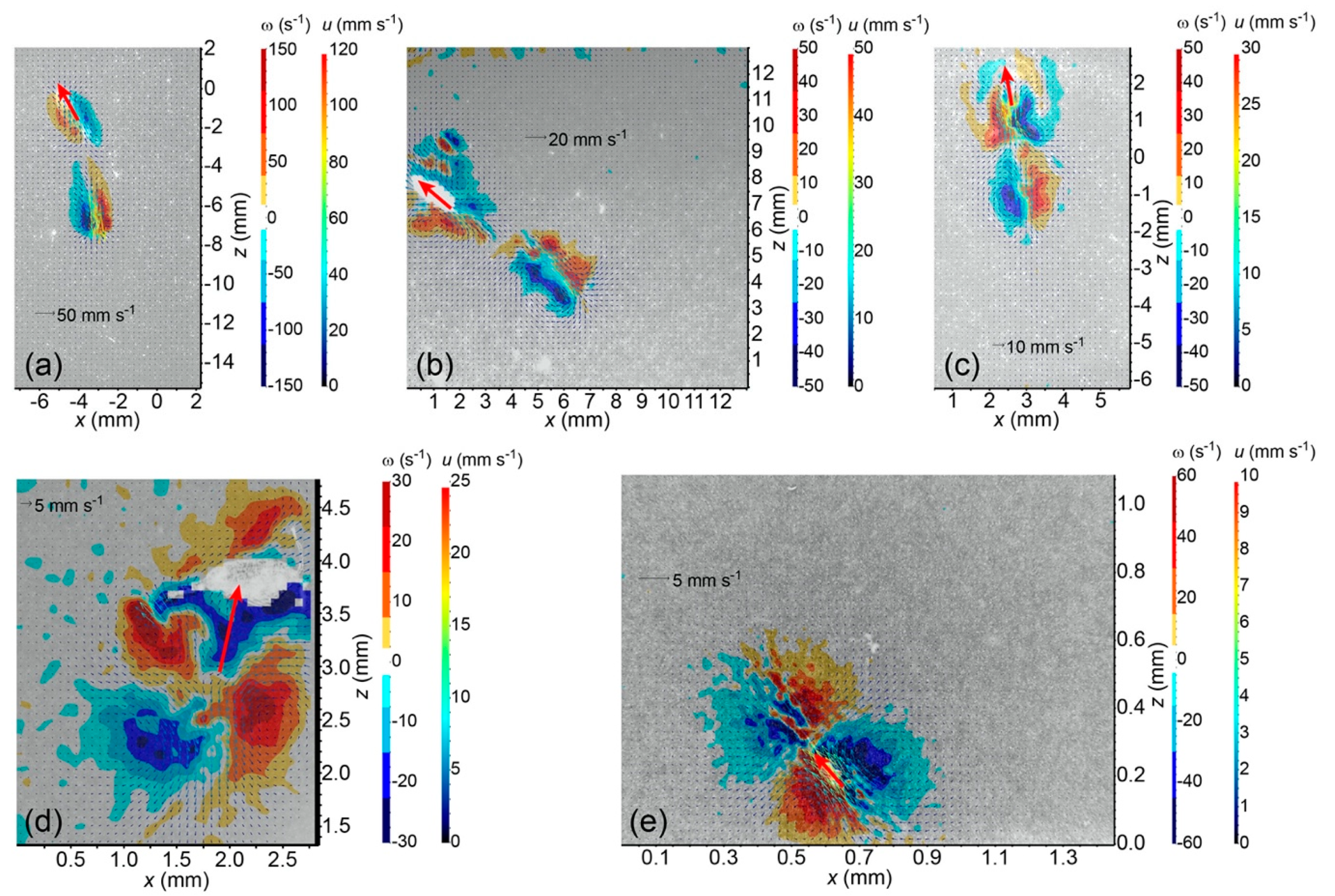
For real cases of plankton jumping, time-resolved PIV measured circulation data are fitted to the above-mentioned viscous vortex ring models to determine t*. Results of t* are then used to calculate the Froude propulsion efficiencies from Equation (9) or (10). These include published data for the copepod Acartia tonsa [13,14], the small jellyfish Sarsia tubulosa [16], and the tailed ciliate Pseudotontonia sp. [18], and previously unpublished data for the squid Doryteuthis pealeii paralarvae, the copepod Calanus finmarchicus, and the copepod Acartia hudsonica. The PIV methods have been adequately described previously [13,20].

3. Results

3.1. General Pattern of Jump-Imposed Flow Fields

Jump-imposed flow fields by different plankton species considered in the present study share a similar general pattern that involves two counter-rotating viscous vortex rings of similar intensity, one in the wake and one around the jumping body (Figure 1; Supplementary Video Group S1). The wake vortex ring is generated by the short duration thrust exerted by the plankter’s propulsion machinery on the water. After attaining its maximum speed during a brief accelerating period, the body decelerates due to fluid drag, thereby imparting momentum to the surrounding water and generating the body vortex. Thus, the body vortex lags behind the wake vortex ring roughly by the short duration of thrust.

3.2. Accleration and Deceleration Phases

For all considered species, their jumping can be divided into an acceleration phase and a deceleration phase (Figure 2). In the acceleration phase, the body accelerates from rest to the maximum speed in a short time that is only a small fraction of the viscous timescale. In the deceleration phase, the body decelerates from its maximum speed under the action of fluid drag; the circulation of the wake vortex ring reaches its maximum but lags slightly behind the body attaining its maximum speed; after this, the wake vortex ring decays immediately due to viscosity.

3.3. Jump Number

The jumping plankton species considered in this study have a Reynolds number in the range of 3–300. As the Reynolds number decreases, the nondimensional jump number increases but is always kept smaller than 1 (Figure 3). Of particular interest are the ciliates, Pseudotontonia sp. and Tontonia sp., that have contractible tail-like appendages. They operate at a tail-shrinking time in the range of 2.5–13.4 ms, which is only slightly shorter than the power stroke durations of copepods (6–25 ms). The sizes of the ciliates are at least a few times smaller than those of the copepods; however, the ciliates can increase their effective length scale by deploying a long tail, thereby effectively increasing their viscous timescale to keep their jump number smaller than 1.

3.4. Added Mass Coefficient

The added mass coefficients are calculated from Equation (4) for fast jumping by six plankton species and the calculation results are presented in Table 1. Jumping by the tailed ciliate Pseudotontonia sp. has an extremely high added mass coefficient of a mean value of 41.0. Relocating jumping by the copepod Acartia tonsa has an added mass coefficient of 0.26 ± 0.24 (SD). An extremely fast jump by a copepod Calanus finmarchicus has an added mass coefficient of 1.60 (Example 2 of Supplementary Video Group S1), while an oblique relocating jump by a copepod A. hudsonica female has an added mass coefficient of 1.96 (Example 4 of Supplementary Video Group S1). Jumping by the squid Doryteuthis pealeii paralarvae has an added mass coefficient of 3.19 ± 1.92 (SD). Jumping by the small medusa Sarsia tubulosa has an added mass coefficient of 0.49 ± 0.34 (SD).

3.5. Froude Propulsion Efficiency

The Froude propulsion efficiencies are calculated from Equation (9) or (10) for fast jumping by six plankton species and the calculation results are presented in Table 2. Jumping by the tailed ciliate Pseudotontonia sp. has a high Froude propulsion efficiency of 0.904. Copepod jumping also has a high Froude propulsion efficiency, usually >0.95, except for an oblique relocating jump by Acartia hudsonica (0.737; Example 4 of Supplementary Video Group S1). Jumping by the squid Doryteuthis pealeii paralarvae has a Froude propulsion efficiency of 0.436 ± 0.158 (SD). Jumping by the small medusa Sarsia tubulosa has a Froude propulsion efficiency of 0.377 ± 0.259 (SD).
Figure 4 shows the functional dependencies of both ηiStokeslet and ηistresslet on R ν t * and of ηHill on R/a (Equations (9)–(11)). For a given α (e.g., α = 0.5; Figure 4), both ηiStokeslet and ηistresslet decrease as R ν t * increases; since R is the equivalent spherical radius of the body, i.e., a body size scale, while ν t * is a size scale for the imposed wake vortex ring when it attains its largest circulation, increasing R ν t * means decreasing the size of the wake vortex ring at its maximum circulation. Additionally, ηHill decreases as R/a increases; since a is the radius of the Hill’s spherical vortex, increasing R/a means decreasing the size of the wake vortex ring.
The Froude propulsion efficiency (η) also depends on the nondimensional kinetic energy of the wake vortex ring (κ). Since κ iStokeslet = 2 12 0.118 is very close to κ istresslet = π 20 2 0.111 , ηiStokeslet and ηistresslet are almost identical for given α and R ν t * (e.g., α = 0.5; Figure 4). Because κ Hill = 10 π 35 0.160 is larger than both κiStokeslet and κistresslet, ηHill is always smaller than both ηiStokeslet and ηistresslet for given α and R ν t *   = R/a (Figure 4).
The Froude propulsion efficiency (η) also depends on the added mass term ( ρ body ρ water + α ) in Equations (8)–(11). For ρ body ρ water = 1 , as α increases (e.g., α = 0.5 versus α = 2.0; Figure 4), ηiStokeslet, ηistresslet, and ηHill all decrease. For ρ body ρ water 1 , the denser the body relative to the seawater, the smaller the Froude propulsion efficiency.

4. Discussion

For jumps of a few species considered in this study, the Froude propulsion efficiencies calculated using the newly developed elastic collision model can be compared to available previous results obtained using completely different methods. The Froude propulsion efficiencies calculated in the present study for jumps of the copepods Acartia tonsa and Calanus finmarchicus (Table 2) compare well to the previous CFD simulation results that range from 0.94 to 0.98 [21]. The present calculation results of Froude propulsion efficiencies for the squid Doryteuthis pealeii paralarvae are 0.436 ± 0.158 (SD), ~42% smaller than the previous results of 0.749 ± 0.009 (SD) calculated using PIV-measured jet properties [24]; however, the previous study used 15 Hz for PIV data acquisition, which was not enough to temporally resolve the fast-evolving flow, compared with 1000 Hz for time-resolved PIV in the present study. Nevertheless, these fairly good comparisons suggest that the present elastic collision model captures reasonably well the fluid physics underlying fast jumping motions of many small planktonic organisms. The brief and nearly impulsive acceleration phase for the jumping body to attain its maximum speed can be regarded as a nearly inviscid process, and the jumping body with added mass and its imposed wake vortex ring can be considered as two particles that separate elastically from each other.
The added mass coefficients for jumping by six plankton species have also been estimated from experimental data. To the author’s best knowledge, these are the first estimations of added mass coefficients for self-propelled jumping plankters. The estimated added mass coefficients differ generally from that of a towed accelerating sphere (i.e., 0.5), varying significantly for plankton species that differ in size, morphology, and propulsion machinery. The ciliate Pseudotontonia sp. deploys a long tail and shrinks it rapidly to accelerate a large amount of the surrounding water, thereby having an extremely high added mass coefficient (~41.0); this extremely high added mass coefficient may be an overestimation but could also be possible because of the big size difference between the cell’s main body (~90 μm in length) and the sub-cellular tail that is the propulsion machinery (290–900 μm in length). The relatively high added mass coefficient (~3.19) calculated for the squid Doryteuthis pealeii paralarva probably is an overestimation as the effect due to the excess weight of the paralarva should not be neglected in Equation (3). Copepods have a wide range of the added mass coefficient (0.05–1.96), probably because of their teardrop body shapes and versatile jumping behaviors. The highly deformable body shape of the small medusa Sarsia tubulosa likely leads to its relatively low added mass coefficient (~0.49). The added mass coefficient is an important parameter that affects the mechanical energy cost and efficiency and imposed flow-field of plankton jumping. The term ( ρ body ρ water + α ) that represents the added-mass effects appears explicitly in Equations (8)–(11) for calculating the Froude propulsion efficiency. The Froude propulsion efficiency decreases as body mass density increases relative to seawater mass density and as the added mass coefficient increases. More research, however, is still needed to shed light on how plankton’s morphological and behavioral traits determine their added mass coefficients and in turn how their added mass coefficients affect their individual-level ecological tasks such as jumping and predator–prey interactions.
The Froude propulsion efficiency decreases as the nondimensional kinetic energy of the wake vortex ring increases. A viscous vortex ring (pair) generated by an impulsive Stokeslet (stresslet) has a considerably smaller nondimensional kinetic energy than an inviscid vortex ring such as a Hill’s spherical vortex (Equations (7), (A9), (A18), and (A28)). Hence, for given impulse I and circulation Γ, to generate an impulsive viscous vortex ring requires less kinetic energy K than to generate a Hill’s spherical vortex. It is not unreasonable to assume that, at the end of the acceleration phase of a jump, the size of the imposed wake vortex ring is similar to the size of the jumping body. For the wake vortex ring to be approximated by an impulsive Stokeslet or stresslet, this assumption means R ν t * = 1, and therefore the Froude propulsion efficiency ηiStokeslet = 0.968 (Equation (9) and assuming α = 0.5) or ηistresslet = 0.970 (Equation (10) and assuming α = 0.5). In contrast, for the wake vortex ring to be approximated by a Hill’s spherical vortex, this assumption means R/a = 1, and therefore ηHill = 0.412 (Equation (11) and assuming α = 0.5), which is significantly lower. Thus, by the very nature of the viscous vortex ring, impulsive jumping by small plankters is an energetically efficient propulsion mode.
The specific way by which a jumping plankter generates a viscous wake vortex ring makes a difference to the Froude propulsion efficiency of its jumping motion. Copepods such as Acartia tonsa and Calanus finmarchicus beat their swimming legs to generate the viscous wake vortex, and usually they also bend their urosome to aid this process. As a result, their appendage beating movements arrange the imparted momentum on the water in such a way that a well-developed, large viscous vortex ring is generated at the end of the acceleration phase of jumping, thereby achieving R ν t * < 1 to ensure a high Froude propulsion efficiency. In contrast, being constrained by their evolutionary history, the squid Doryteuthis pealeii paralarvae use their jet funnel of ~0.2 mm orifice diameter to deliver momentum on the water. As a result, only a compact, prototype viscous vortex is generated at the end of the acceleration phase, thereby causing R ν t * > 1 to end up with a relatively low Froude propulsion efficiency. The small jellyfish Sarsia tubulosa contracts its bell to initially generate a viscous wake vortex ring; however, likely for feeding purposes, the subsequent bell relaxation draws water into the bell cavity (Example 3 of Supplementary Video Group S1). As a result, the development of the wake vortex ring is arrested to some degree, leading to a low Froude propulsion efficiency. These understandings are visually and qualitatively consistent with available PIV measured instantaneous vorticity fields when circulations reach their maximum.
The overall size of the viscous vortex ring pair generated by the ciliate Pseudotontonia sp. is significantly larger than its body size (Figure 1e), because the ciliate boosts its effective length scale by deploying a long, tail-like, sub-cellular structure, and its jumping is accompanied by an extremely high added mass coefficient. This seems to contradict the suggestion that the imposed viscous vortex ring pair helps to reduce the predation risk due to a flow-sensing predator [18]. An alternative explanation may be that the ciliate imposes the viscous vortex ring pair to mimic the presence of copepods that are common predators of protists, thereby scaring away other protistan grazers to reduce feeding competition on algae.
Finally, the present study has applied two Stokes flow models, i.e., the impulsive Stokeslet and stresslet, to plankton jumping flows of Reynolds numbers in the range of 3–300. This is only practically justified by the fact that the decay-phase circulation fits very well to either one of the two models. The authors of [25] investigated partially the effect due to a small, finite Reynolds number on the time evolution of an axisymmetric vortex ring by solving the linearized vorticity equation (i.e., the Stokes approximation). The analytical solution was obtained for an initial condition different from the way a plankton jumping flow is generated, and no closed-form expression is available for the impulse of the vortex ring. Thus, it is difficult to apply this theoretical model to plankton jumping flows. It remains an interesting problem to investigate the finite Reynolds number effects on plankton jumping flows.

Supplementary Materials

The following are available online at https://www.mdpi.com/2311-5521/5/3/154/s1. Supplementary Video Group S1: Five examples of fast jumping motions of plankton that are propelled by generating impulsive viscous vortex rings. Supplementary Video Group S2: Animations of the flow fields and vorticity fields of an impulsive Stokeslet, an impulsive stresslet, and a Hill’s spherical vortex.

Funding

This research was funded by US National Science Foundation, grant numbers OCE-1559062 and IOS-1353937, to H.J.

Acknowledgments

The author would like to thank T. Kiørboe, S. Colin, B. Gemmell, E. Buskey, and K. Katija for collaboration on investigating the jumping mechanisms of some of the plankton species that are considered in this manuscript. The author thanks three anonymous reviewers for providing helpful and constructive comments that improved the manuscript.

Conflicts of Interest

The author declares no conflict of interest.

Appendix A. The Impulsive Stokeslet

An impulsive Stokeslet [13] consists of a point momentum source of magnitude ρI, where ρ is the mass density of the fluid and I is the hydrodynamic impulse, acting only impulsively for a very short period of time, formally represented by the Dirac delta function δ(t). In a cylindrical polar coordinate system (x, r, φ) where x, r, and φ are respectively the axial, radial, and azimuthal coordinate, the azimuthal vorticity (ωφ) and Stokes streamfunction (Ψφ) for the flow imposed by an impulsive Stokeslet are, respectively,
ω ϕ ( x , r , t ) = I   r 16 π 3 / 2   ( ν t ) 5 / 2   e ξ 2
Ψ ϕ ( x , r , t ) = I   r 2 2 π 3 / 2   ( x 2 + r 2 ) 3 / 2   ( π 2 erf ( ξ ) ξ e ξ 2 )
where ξ = x 2 + r 2 4 ν t , ν is fluid kinematic viscosity, and the error function erf ( ξ ) = 2 π 0 ξ e y 2 d y .
The axial (u) and radial (v) velocity components are
u ( x , r , t ) 1 r Ψ ϕ r = I 2 π 3 / 2 ( 2 x 2 r 2 ) A 1 + 2 r 2 A 2 ( x 2 + r 2 ) 5 / 2
v ( x , r , t ) 1 r Ψ ϕ x = I 2 π 3 / 2 x r ( 3 A 1 2 A 2 ) ( x 2 + r 2 ) 5 / 2
where A 1 = π 2 erf ( ξ ) ξ e ξ 2 and A 2 = ξ 3 e ξ 2 . At small time, the far field (i.e., ξ >> 1) of the flow is approximately irrotational (potential) and behaves as
u = I 4 π 2 x 2 r 2 ( x 2 + r 2 ) 5 / 2
v = I 4 π 3 x r ( x 2 + r 2 ) 5 / 2
and the associated velocity magnitude is
U iStokeslet u 2 + v 2 = I 4 π 4 x 2 + r 2 ( x 2 + r 2 ) 2
The circulation (Γ), impulse (I), and kinetic energy (K) of the viscous vortex ring imposed by the impulsive Stokeslet are, respectively,
Γ ( t ) 0 + + ω ϕ d x   d r = I π ( 4 ν t )
I ( t ) π 0 + + ω ϕ r 2 d x   d r = I
K ( t ) π 0 + + ω ϕ Ψ ϕ d x   d r = 2 12 I 2 π 3 / 2 ( 4 ν t ) 3 / 2
The nondimensional kinetic energy of the viscous vortex ring imposed by the impulsive Stokeslet is
κ iStokeslet K I 1 / 2   Γ 3 / 2 = 2 12 0.118
An animation of the flow field and vorticity field of an impulsive Stokeslet is shown in Supplementary Video Group S2.

Appendix B. The Impulsive Stresslet

An impulsive stresslet [14] consists of two point momentum sources of equal magnitude (ρI), acting synchronously in opposite direction and separated by distance ε; each momentum source acts impulsively for a very short period of time, formally represented by δ(t). The definition of the strength of the impulsive stresslet is M ≡ limε→0,I→∞() = constant.
The azimuthal vorticity (ωφ) and Stokes streamfunction (Ψφ) for the flow imposed by an impulsive stresslet are, respectively,
ω ϕ ( x , r , t ) = M   x   r 32 π 3 / 2   ( ν t ) 7 / 2   e ξ 2
Ψ ϕ ( x , r , t ) = 3 M   x   r 2 2 π 3 / 2   ( x 2 + r 2 ) 5 / 2   [ π 2 erf ( ξ ) + ξ e ξ 2 ( 1 + 2 3 ξ 2 ) ]
The axial (u) and radial (v) velocity components are
u ( x , r , t ) 1 r Ψ ϕ r = M 2 π 3 / 2 x [ ( 2 x 2 3 r 2 ) B 1 + r 2 B 2 ] ( x 2 + r 2 ) 7 / 2
v ( x , r , t ) 1 r Ψ ϕ x = M 2 π 3 / 2 r [ ( r 2 4 x 2 ) B 1 + x 2 B 2 ] ( x 2 + r 2 ) 7 / 2
where B 1 = 3 [ π 2 erf ( ξ ) + ξ e ξ 2 ( 1 + 2 3 ξ 2 ) ] and B 2 = 4 ξ 5 e ξ 2 . At small time, the far field (i.e., ξ >> 1) of the flow is approximately irrotational (potential) and behaves as
u = 3 M 4 π x ( 2 x 2 3 r 2 ) ( x 2 + r 2 ) 7 / 2
v = 3 M 4 π r ( 4 x 2 r 2 ) ( x 2 + r 2 ) 7 / 2
and the associated velocity magnitude is
U istresslet u 2 + v 2 = 3 M 4 π 4 x 4 + r 4 ( x 2 + r 2 ) 3
The circulation (Γ), impulse (I), and kinetic energy (K) of each component of the viscous vortex ring pair imposed by the impulsive stresslet are, respectively,
Γ ( t ) 0 + 0 + ω ϕ d x   d r = M π 3 / 2 ( 4 ν t ) 3 / 2
I ( t ) π 0 + 0 + ω ϕ r 2 d x   d r = M π 1 / 2 ( 4 ν t ) 1 / 2
K ( t ) π 0 + 0 + ω ϕ Ψ ϕ d x   d r = 1 20 2 M 2 π 3 / 2 ( 4 ν t ) 5 / 2
The nondimensional kinetic energy of each component of the viscous vortex ring pair imposed by the impulsive stresslet is
κ istresslet K I 1 / 2   Γ 3 / 2 = π 20 2 0.111
An animation of the flow field and vorticity field of an impulsive stresslet is shown in Supplementary Video Group S2.

Appendix C. Hill’s Spherical Vortex

Hill’s spherical vortex is an axisymmetric vortex ring with the strength of the vorticity within the vortex proportional to the distance from the axis of traveling (e.g., [26,27]). That is, in a cylindrical polar coordinate system (x, r, φ) with the positive axial (x-) direction coinciding with the traveling direction, the azimuthal vorticity is given by ωφ = C r, where C is a constant. Outside the vortex, the vorticity vanishes, and the flow is identical to that for uniform irrotational flow due to the translation of a sphere.
In a stationary frame of reference, the Stokes streamfunction inside and outside Hill’s spherical vortex of radius a is given by
Ψ in ( x , r , t ) = U 2 r 2 + C 10 r 2 [ a 2 ( x U t ) 2 r 2 ]
Ψ out ( x , r , t ) = U 2 r 2 U 2 r 2 { 1 a 3 [ ( x U t ) 2 + r 2 ] 3 / 2 }
where U = 2Ca2/15, which is the vortex translation velocity.
Within the vortex, the axial (uin) and radial (vin) velocity components are
u in ( x , r , t ) 1 r Ψ in r = U + C 5 [ a 2 ( x U t ) 2 2 r 2 ]
v in ( x , r , t ) 1 r Ψ in x = C 5 r ( x U t )
Outside the vortex, the axial (uout) and radial (vout) velocity components are
u out ( x , r , t ) 1 r Ψ out r = U a 3 2 ( x U t ) 2 r 2 2 [ ( x U t ) 2 + r 2 ] 5 / 2
v out ( x , r , t ) 1 r Ψ out x = U a 3 3 r ( x U t ) 2 [ ( x U t ) 2 + r 2 ] 5 / 2
and the associated velocity magnitude is
U out u out 2 + v out 2 = U a 3 4 ( x U t ) 2 + r 2 2 [ ( x U t ) 2 + r 2 ] 2
The circulation (Γ), impulse (I), and kinetic energy (K) of Hill’s spherical vortex are, respectively,
Γ 0 + + ω ϕ d x   d r = 5 U a
I π 0 + + ω ϕ r 2 d x   d r = 2 π a 3 U
K π 0 + + ω ϕ Ψ d x   d r = 10 7 π a 3 U 2
The nondimensional kinetic energy of Hill’s spherical vortex is
κ Hill K I 1 / 2   Γ 3 / 2 = 10 π 35 0.160
An animation of the flow field and vorticity field of a Hill’s spherical vortex is shown in Supplementary Video Group S2.

References

  1. Osborn, T. The role of turbulent diffusion for copepods with feeding currents. J. Plankton Res. 1996, 18, 185–195. [Google Scholar] [CrossRef] [Green Version]
  2. Lazier, J.R.N.; Mann, K.H. Turbulence and diffusive layers around small organisms. Deep Sea Res. 1989, 36, 1721–1733. [Google Scholar] [CrossRef]
  3. Koehl, M.A.R.; Strickler, J.R. Copepod feeding currents: Food capture at low Reynolds number. Limnol. Oceanogr. 1981, 26, 1062–1073. [Google Scholar] [CrossRef] [Green Version]
  4. Strickler, J.R. Sticky water: A selective force in copepod evolution. In Trophic Interactions within Aquatic Ecosystems; Meyers, D.G., Strickler, J.R., Eds.; AAAS Selected Symposium 85, American Association for the Advancement of Science; Westview Press: Boulder, CO, USA, 1984; pp. 187–239. [Google Scholar]
  5. Yen, J.; Strickler, J.R. Advertisement and concealment in the plankton: What makes a copepod hydrodynamically conspicuous? Invertebr. Biol. 1996, 115, 191–205. [Google Scholar] [CrossRef] [Green Version]
  6. Jiang, H.; Osborn, T.R. Hydrodynamics of copepods: A review. Surv. Geophys. 2004, 25, 339–370. [Google Scholar] [CrossRef]
  7. Kiørboe, T. A Mechanistic Approach to Plankton Ecology; Princeton University Press: Princeton, NJ, USA, 2008. [Google Scholar]
  8. Herfort, L.; Peterson, T.D.; McCue, L.A.; Crump, B.C.; Prahl, F.G.; Baptista, A.M.; Campbell, V.; Warnick, R.; Selby, M.; Roegner, G.C.; et al. Myrionecta rubra population genetic diversity and its cryptophyte chloroplast specificity in recurrent red tides in the Columbia River estuary. Aquat. Microb. Ecol. 2011, 62, 85–97. [Google Scholar] [CrossRef] [Green Version]
  9. Garcia-Cuetos, L.; Moestrup, Ø.; Hansen, P.J. Studies on the genus Mesodinium II. Ultrastructural and molecular investigations of five marine species help clarifying the taxonomy. J. Eukaryot. Microbiol. 2012, 59, 374–400. [Google Scholar] [CrossRef] [PubMed]
  10. Johnson, M.D.; Beaudoin, D.J.; Laza-Martinez, A.; Dyhrman, S.T.; Fensin, E.; Lin, S.; Merculief, A.; Nagai, S.; Pompeu, M.; Setälä, O.; et al. The genetic diversity of Mesodinium and associated cryptophytes. Front. Microbiol. 2016, 7, 2017. [Google Scholar] [CrossRef]
  11. Jiang, H. Why does the jumping ciliate Mesodinium rubrum possess an equatorially located propulsive ciliary belt? J. Plankton Res. 2011, 33, 998–1011. [Google Scholar] [CrossRef] [Green Version]
  12. Jiang, H.; Johnson, M.D. Jumping and overcoming diffusion limitation of nutrient uptake in the photosynthetic ciliate Mesodinium rubrum. Limnol. Oceanogr. 2017, 62, 421–436. [Google Scholar] [CrossRef]
  13. Kiørboe, T.; Jiang, H.; Colin, S.P. Danger of zooplankton feeding: The fluid signal generated by ambush-feeding copepods. Proc. R. Soc. B 2010, 277, 3229–3237. [Google Scholar] [CrossRef] [PubMed]
  14. Jiang, H.; Kiørboe, T. The fluid dynamics of swimming by jumping in copepods. J. R. Soc. Interface 2011, 8, 1090–1103. [Google Scholar] [CrossRef] [PubMed] [Green Version]
  15. Murphy, D.W.; Webster, D.R.; Yen, J. A high-speed tomographic PIV system for measuring zooplanktonic flow. Limnol. Oceanogr. Methods 2012, 10, 1096–1112. [Google Scholar] [CrossRef] [Green Version]
  16. Katija, K.; Jiang, H. Swimming by medusae Sarsia tubulosa in the viscous vortex ring limit. Limnol. Oceanogr. Fluids Environ. 2013, 3, 103–118. [Google Scholar] [CrossRef] [Green Version]
  17. Wadhwa, N.; Andersen, A.; Kiørboe, T. Hydrodynamics and energetics of jumping copepod nauplii and copepodids. J. Exp. Biol. 2014, 217, 3085–3094. [Google Scholar] [CrossRef] [Green Version]
  18. Gemmell, B.J.; Jiang, H.; Buskey, E.J. A tale of the ciliate tail: Investigation into the adaptive significance of this sub-cellular structure. Proc. R. Soc. B 2015, 282, 20150770. [Google Scholar] [CrossRef] [Green Version]
  19. Skipper, A.N.; Murphy, D.W.; Webster, D.R. Characterization of hop-and-sink daphniid locomotion. J. Plankton Res. 2019, 41, 142–153. [Google Scholar] [CrossRef]
  20. Jiang, H.; Paffenhöfer, G.-A. Vortical feeding currents in nauplii of the calanoid copepod Eucalanus pileatus. Mar. Ecol. Prog. Ser. 2020, 638, 51–63. [Google Scholar] [CrossRef]
  21. Jiang, H.; Kiørboe, T. Propulsion efficiency and imposed flow fields of a copepod jump. J. Exp. Biol. 2011, 214, 476–486. [Google Scholar] [CrossRef] [Green Version]
  22. Lighthill, M.J. Aquatic animal propulsion of high hydromechanical efficiency. J. Fluid Mech. 1970, 44, 265–301. [Google Scholar] [CrossRef]
  23. Lighthill, J. An Informal Introduction to Theoretical Fluid Mechanics; Clarendon Press: Oxford, UK, 1986. [Google Scholar]
  24. Bartol, I.K.; Krueger, P.S.; Stewart, W.J.; Thompson, J.T. Pulsed jet dynamics of squid hatchlings at intermediate Reynolds numbers. J. Exp. Biol. 2009, 212, 1506–1518. [Google Scholar] [CrossRef] [PubMed] [Green Version]
  25. Fukumoto, Y.; Kaplanski, F. Global time evolution of an axisymmetric vortex ring at low Reynolds numbers. Phys. Fluids 2008, 20, 053103. [Google Scholar] [CrossRef]
  26. Lim, T.T.; Nickels, T.B. Vortex rings. In Fluid Vortices; Green, S.I., Ed.; Kluwer Academic Publishers: Dordrecht, The Netherlands, 1995; pp. 95–153. [Google Scholar]
  27. Pozrikidis, C. Introduction to Theoretical and Computational Fluid Dynamics; Oxford University Press: Oxford, UK, 1997. [Google Scholar]
Figure 1. Time-resolved PIV measurements of jump-imposed instantaneous flow velocity vector and vorticity fields by (a) a squid Doryteuthis pealeii paralarva, (b) a copepod Calanus finmarchicus, (c) a small medusa Sarsia tubulosa (PIV data were obtained by [16]), (d) a copepod Acartia hudsonica female, and (e) a ciliate Pseudotontonia sp. (PIV data were obtained by [18]). The filled color contours are vorticity fields. The velocity vectors are colored by flow velocity magnitudes. In each panel, the solid red arrow indicates the jumping direction of the body. Details of the events are presented by Supplementary Video Group S1.
Fluids 05 00154 g001
Figure 2. Time evolutions of the time-resolved PIV measured circulations (Γ) of the wake vortex ring, fitted decay-phase circulations (Γ) to the impulsive Stokeslet model, and body speeds (U) for jumps by (a) a squid Doryteuthis pealeii paralarva, (b) a copepod Calanus finmarchicus, (c) a small medusa Sarsia tubulosa (data were obtained by [16]), (d) a copepod Acartia hudsonica female, and (e) a ciliate Pseudotontonia sp. (data were obtained by [18]). The cases presented here are respectively corresponding to those presented in Figure 1. Time (t) is scaled by the viscous timescale τν = L2/(4ν), where L is the body length for (ad); for (e), L = (body length + tail length)/2. In the initial acceleration phase that is approximately inviscid, the wake vortex circulation increases from 0 at 0 ms to its maximum value roughly at the time τ (i.e., the thrust duration) through the action of thrust and stretching and tilting of vortex lines; thus, the viscous solution of the impulsive Stokeslet model does not apply to this phase. In contrast, in the deceleration phase, the wake vortex circulation stops growing but decays under the action of viscosity; thus, the circulation fit using the impulsive Stokeslet model only covers the decay-phase circulation data starting from the maximum circulation. As to the question of why here the decay-phase circulations are fitted to the impulsive Stokeslet model and not the impulsive stresslet model, previous data analyses have shown that the flow imposed by a relocating copepod A. tonsa [14] and by a hopping Daphnia magna [19] can be better described by the impulsive stresslet model, while the jumping flow imposed by a small medusa S. tubulosa [16] and by a ciliate Pseudotontonia sp. [18] can be better described by the impulsive Stokeslet model. Similar data analyses also suggest that the impulsive stresslet model is not a better model for the jumping flow imposed by a squid D. pealeii paralarva, by a copepod C. finmarchicus, or by a copepod A. hudsonica female (not shown for brevity). Thus, here, the decay-phase circulations are fitted to the impulsive Stokeslet model for the five species whose jumping flows are better described by the impulsive Stokeslet model.
Fluids 05 00154 g002
Figure 3. The nondimensional jump number (Njump) as a function of the Reynolds number (ReUmax L/ν, where Umax is the maximum jumping speed, L = (body length + tail length)/2 for Pseudotontonia and Tontonia, and L = body length for all other species). For the copepod Acartia tonsa, data were obtained by [13]. For the small medusa Sarsia tubulosa, data were obtained by [16]. For the ciliates Pseudotontonia sp. and Tontonia sp., data were obtained by [18].
Fluids 05 00154 g003
Figure 4. Froude propulsion efficiency η as a function of R ν t * based on the impulsive Stokeslet model (Equation (9)) or the impulsive stresslet model (Equation (10)) or as a function of R/a based on the model of Hill’s spherical vortex (Equation (11)). For the impulsive Stokeslet model and the model of Hill’s spherical vortex, two values of the added mass coefficient are considered, i.e., α = 0.5 or 2.0, while for the impulsive stresslet model, α = 0.5 is considered. All calculations assume ρbody/ρwater = 1.
Fluids 05 00154 g004
Table 1. Summary of the calculation results of the added mass coefficient.
Pseudotontonia sp.Acartia tonsaAcartia hudsonicaCalanus finmarchicusSquid ParalarvaeSmall Sarsia tubulosa
Mean41.00.261.961.603.190.49
±SD-±0.24--±1.92±0.34
Range37.07–44.920.05–0.53--0.46–6.220.12–0.93
n251194
All calculations assume ρbody/ρwater = 1.
Table 2. Summary of the calculation results of the Froude propulsion efficiency.
Pseudotontonia sp.Acartia tonsa1Acartia hudsonicaCalanus finmarchicus2Squid ParalarvaeSmall Sarsia tubulosa
Mean0.9040.9880.7370.9530.4360.377
±SD-±0.009--±0.158±0.259
Range0.900–0.9070.974–0.997-0.953–0.9530.187–0.6750.231–0.764
n251294
1 Calculated using Equation (10) for the impulsive stresslet. All other calculations used Equation (9) for the impulsive Stokeslet. 2 An added mass coefficient 1.60 was used for both cases.

