Article

On the Optimal Control of Stationary Fluid–Structure Interaction Systems

Department of Industrial Engineering, Lab. of Montecuccolino, University of Bologna, Via dei Colli 16, 40136 Bologna, Italy
*
Author to whom correspondence should be addressed.
Fluids 2020, 5(3), 144; https://doi.org/10.3390/fluids5030144
Submission received: 3 June 2020 / Revised: 4 August 2020 / Accepted: 25 August 2020 / Published: 28 August 2020
(This article belongs to the Special Issue Classical and Modern Topics in Fluid Dynamics and Transport Phenomena)

Abstract

:
Fluid–structure interaction (FSI) systems consist of a fluid which flows and deforms one or more solid surrounding structures. In this paper, we study inverse FSI problems, where the goal is to find the optimal value of some control parameters, such that the FSI solution is close to a desired one. Optimal control problems are formulated with Lagrange multipliers and adjoint variables formalism. In order to recover the symmetry of the stationary state-adjoint system an auxiliary displacement field is introduced and used to extend the velocity field from the fluid into the structure domain. As a consequence, the adjoint interface forces are balanced automatically. We present three different FSI optimal controls: inverse parameter estimation, boundary control and distributed control. The optimality system is derived from the first order necessary condition by taking the Fréchet derivatives of the augmented Lagrangian with respect to all the variables involved. The optimal solution is obtained through a gradient-based algorithm applied to the optimality system. In order to support the proposed approach and compare these three optimal control approaches numerical tests are performed.

1. Introduction

Optimization has always been a key aspect in the field of engineering in order to improve the performance of an existing design or to improve its capability. As long as the goals to pursue are trivial, improvements can be attained by trial and error without the use of sophisticated mathematical models. When the problem becomes complex, the use of the appropriate optimization techniques is instead essential. There are many approaches to optimal control problems that range from genetic algorithms to adjoint methods. In this paper, we consider adjoint based methods since they have a solid mathematical background. This mathematical approach allow us to evaluate the well-posedness of the problem, the existence of local optimal solutions and the investigation of several numerical convergence issues. The interested reader can see [1] and citations therein. Adjoint solvers have commonly been implemented in commercial software, such as ANSYS, but the exact solution of an optimal problem remains a difficult task due to the definition of appropriate solution spaces and differentiability issues. Usually, optimal solutions lie in distributional spaces and the correct numerical representations can be found only with appropriate regularizations. When the solution space is well-defined and the control problem differentiable, then the adjoint methods have been proven to be good tools for the optimal control of fluid dynamics complex problems, see, for example, [2,3].
Multidimensional phenomena, which depend both on time and space, are often modeled by mean of partial differential equations including heat and wave propagation, electrodynamics, quantum mechanics, fluid and solid motion. In fluid–structure interaction (FSI) problems the fluid and the solid are coupled into a single problem and the set of partial differential equations describing fluid and solid motion has to be satisfied simultaneously. In this coupling the fluid–structure mutual interaction is fundamental, since the behavior of the solid affects the fluid and vice versa. The fluid, through its pressure, behaves as an external load over the solid structure that deforms and changes the shape of the channel which modifies the fluid dynamic state inside the channel itself. A thorough description of FSI forward problems can be found in many interesting books, see, for example, [4,5,6,7]. Commercial packages, which use segregate solvers to speed up the convergence and reduce memory consumption, are commonly used for complex FSI real-life simulations. However, partitioned formulations frequently show convergence problems that are often overtaken with limiters.
Conversely, in the monolithic variational formulation, the fluid-solid coupling conditions, which are the main constraints from the fluid to the solid domain, are automatically taken into account and no sub-iterations are necessary as in the case of partitioned approaches, see [8,9,10,11]. The bounds needed by partitioned solvers are a complex matter for optimal control problems that usually exploit near-singular regions in the optimization process. In many optimal cases and engineering applications, it is not necessary to reach the minimum and only a few iterations are enough to improve the design. The segregated solvers, with their limiters, can cope with a couple of optimal subiterations but more robust monolithic solvers are necessary for benchmarks and for developing correct answers.
Monolithic FSI solvers require high amounts of computational resources but multigrid and domain decomposition methods have successfully reduced the gap with segregated solvers for the solution of large sparse coupled linear systems. The reader interested in a detailed analysis of multigrid methods can refer to [12,13]. These methods have gained great popularity within the FSI community and a multitude of studies have been published in recent years. Two-dimensional FSI problems are solved in [14] by using Vanka-type smoothers in the multigrid cycle while an extension to three-dimensional domains is presented in [15], where the smoother is obtained by splitting the coupled problem into a fluid and a solid domain. In the same work, the authors also consider a simplified FSI model in order to prove by Fourier analysis that multigrid successfully damps high frequency errors. In [16] the authors use a geometric multigrid preconditioner combined with domain decomposition smoothers for monolithic Newton–Krylov solvers. They show good results also in the case of incompressible materials and direct-to-steady FSI simulations. Finally, in the recent work [17] the authors show the efficiency and scalability of a parallel approximated Newton multigrid solver for monolithic FSI.
Many FSI studies have been published in recent years but the optimal control of such problems is still an open challenge. In many cases the “trial and fail” technique is still the most used optimal control tool. Only few optimal control studies of FSI systems can be found in literature. Among them the reader can see [18,19,20,21,22,23]. The authors in [18] study a linear unsteady FSI optimal control problem, written in monolithic form and focus their attention to the theoretical aspects of the problem. The resulting optimality system couples time and space with state and adjoint variables. In order to evaluate the properties of biological tissues, the authors in [19] propose a well-posedness analysis of an inverse FSI problem. Optimal control and parameter estimation of non-stationary and non-linear FSI has been recently investigated in [20]. In [22] a steady Lamé parameter estimation problem and pressure boundary control are studied.
Numerical solutions of realistic unsteady optimality systems, as proposed in [18], are not feasible with the actual computational power, since they couple in space-time the state-adjoint variables. In particular, this coupled optimality system consists of a forward in time equation for the state variables and a backward in time equation for the adjoint variables. The interested reader can see [1] for unsteady optimal control flow problems. In order to reduce the computational effort, we consider the steady optimal control of FSI systems. One of the greatest challenges in the solution of a steady optimal control problem is that the optimal solution, which involves non-linear solid deformations, must be obtained in an iterative way. However, the steady optimality system defines only the steady final configuration with no information on how to balance non-linear intermediate body deformations, interface forces and mesh movements. Following the method described in [21], we introduce an auxiliary displacement field and use it to extend the velocity field to the solid domain. As a consequence, the interface forces both for FSI and adjoint variables are balanced automatically, the fictitious velocity moves the structure and the solid velocity vanishes only at the end of the non-linear iterations.
This paper can be then considered a further development of the idea proposed in [21]. However, in this work we study a larger class of problems than in our previous one where only a boundary pressure control was considered. Here we recover an optimality system that is used to perform boundary pressure control, distributed control or inverse Young modulus estimation with inequality constraints over the control. This is one of the aim of the paper, namely to show that all these different control problems can be solved by the same adjoint approach. Furthermore, in the parameter estimation problems studied in [20,22], the control (i.e., Lamé parameter or Young modulus) is assumed to be constant in the solid subdomain. In this work, we consider instead a spatially non-uniform control. The motivation behind this comes from the growing interest in temperature dependent materials, such as composite materials, where a relationship between the Young modulus and the temperature can easily be established, and the optimal solution can be achieved by controlling the temperature itself. As a consequence, we have to impose inequality constraints on our control parameter, since very high or low values of the Young modulus, and therefore of the temperature, may be physically not meaningful. For the same reasons we also add a regularization on the control, in order to obtain smoother optimal solutions.
The rest of this paper is organized as follows. In Section 2 we describe the FSI model considered. Then, we present three different strategies to solve a displacement matching profile problem in the framework of FSI steady optimization: pressure boundary control, distributed control and finally parameter estimation with inequality constraints. In Section 3 numerical results are presented and finally some conclusions are gathered together.

2. Mathematical Model

In this section we present the formulation of the FSI optimal control problem and recover the optimality system needed to be solved. We first introduce the basic notation about functional spaces. On the open set Ω R m we denote with L 2 ( Ω ) the space of square integrable functions and with H s ( Ω ) the standard Sobolev space with norm · s . We recall that H 0 ( Ω ) = L 2 ( Ω ) and in the following · 0 = · . Let H 0 s ( Ω ) be the space of all functions in H s ( Ω ) that vanish on the boundary of Ω . For more details on these spaces the interested reader can see [12].
Let us consider a bounded open set Ω R n split into a structure domain Ω s and a fluid domain Ω f , so that Ω = Ω s Ω f and Ω s Ω f = . We denote by Γ = Ω the outer boundary, which is then split into solid and fluid boundaries Γ s = Γ Ω s and Γ f = Γ Ω f , respectively. The surface Γ i = Ω s Ω f shared between the solid and the fluid is the fluid–structure interface. The mathematical model of the steady state FSI problem in strong form is defined by the following set of equations
· v = 0 on Ω f ,
ρ f ( v · ) v · σ f = 0 on Ω f ,
· σ s ( η ) = f on Ω s .
The viscous stress tensor σ f of a Newtonian fluid and the Cauchy strain tensor σ s of a St. Venant Kirchhoff material read
σ f ( p , v ) : = p I + μ f ( v + v T ) ,
σ s ( η ) = E S ( η ) = λ s ( · η ) I + μ s ( η + η T ) ,
where p is the fluid pressure, μ f the dynamic viscosity of the fluid while λ s and μ s are the solid Lamé parameters. We denote with η the unknown displacement field and E is the Young modulus. By substituting the following definitions of the Lamé parameters μ s and λ s
μ s = E 2 ( 1 + ν ) λ s = E ν ( 1 + ν ) ( 1 2 ν ) ,
into the (5) we obtain
σ s ( η ) = 1 2 ( 1 + ν ) ( η + η T ) + ν ( 1 + ν ) ( 1 2 ν ) ( · η ) I .
The Young modulus E and Poisson ratio ν determine uniquely the solid physical properties.
In order to complete the FSI problem we need to set the boundary conditions. Let Γ d f and Γ d s be the wall regions where we set Diricet boundary conditions for fluid velocity and solid displacement. Let also Γ n f and Γ n s be part of the boundary where fluid outflow and free displacement boundary conditions are imposed, respectively. The fluid-solid interface is denoted by Γ i . By denoting with n s and n f the normal unit for the solid and fluid boundary on Γ i we summarize the boundary conditions as
v = v 0 on Γ d f , η = η 0 on Γ d s , σ f · n f = 0 on Γ n f , σ s · n s = 0 on Γ n s , σ f · n f + σ s · n s = 0 on Γ i , v = 0 on Γ i .
We remark that, by using a monolithic approach in a finite element framework, the interface conditions are imposed directly in the same solver with correct interface values, see [21,24,25]. In order to simplify notation we introduce the following functional spaces
V = { ϕ H 1 ( Ω ) : ϕ Γ d f Γ d s = 0 } , Q s , f = L 2 ( Ω s , f ) , W s , f = { ϕ H 1 ( Ω ) : ϕ Γ s , f = 0 } .
We rewrite the monolithic FSI system in weak form for the displacement η and for the velocity field v over Ω ( η ) = Ω f ( η ) Ω s ( η ) implicitly incorporating the boundary conditions (8) on the common interface Γ i
Ω f ( · v ) ψ d Ω = 0 ψ Q f , Ω f [ ( ρ f ( v · ) v ) · ϕ p · ϕ + μ f v : ϕ f ] d Ω + Γ [ [ p n f μ f ( v · n f ) · ϕ ] d Γ +
Ω s E ν ( 1 + ν ) ( 1 2 ν ) ( · η ) ( · ϕ ) + 1 2 ( 1 + ν ) η : ϕ d Ω + Γ E 1 2 ( 1 + ν ) ( η · n s ) · ϕ + ν ( 1 + ν ) ( 1 2 ν ) ( · η ) n s · ϕ d Γ = 0 ϕ V ,
The surface integrals vanish due to the boundary and interface conditions (8). If we use standard techniques to obtain the unsteady optimality system for a generic FSI problem in a monolithic form then the adjoint system results in a symmetric and monolithic patterns similar to the unsteady state system. However, if we follow the same standard techniques to obtain the steady optimality then the steady adjoint system results in a non-symmetric and non-monolithic form that differs from those of the state variable Equations (10) and (11). Furthermore, the steady adjoint system results in a set of equations with uncoupled boundary conditions on the interface. In order to have the steady adjoint equations in a similar monolithic form, with coupled boundary conditions as well, we need to extend the state variables appropriately. Over the solid domain Ω s ( η ) we define the auxiliary displacement field η ^ , solution of the following Laplace operator and boundary conditions
2 η ^ = 0 x Ω s ,
η ^ = η on Γ i ,
η ^ = 0 on ( Ω s Γ i ) .
Therefore, over the whole domain Ω , we can define the velocity field v as
v = τ ( η η ^ ) on Ω s ( η ) v solution   of ( 1 ) ( 2 ) on Ω f ( η ) ,
with τ a constant that mimics the time behavior. The mapping η ^ : Ω s ( 0 ^ ) Ω s ( η ^ ) defines the solid domain movement. Over Γ i , the velocity field v is set to be continuous during the non-linear optimal control iterations and vanishes as the algorithm reaches the steady state. The introduction of the velocity field v allows us to differentiate the functional and take the shape derivatives of Ω s ( η ^ ) and Ω f ( η ^ ) . With this notation the FSI problem takes the following form
Ω f ( η ^ ) ( · v ) ψ d Ω = 0 ψ Q f ,
Ω s ( η ^ ) E 1 2 ( 1 + ν ) η : ϕ + ν ( 1 + ν ) ( 1 2 ν ) ( · η ) ( · ϕ ) f d Ω + Ω f ( η ^ ) [ ( ρ f ( v · ) v ) · ϕ p · ϕ + μ f v : ϕ ] d Ω = 0 ϕ V ,
Ω s ( η ^ ) η ^ : η ^ a d Ω = 0 η ^ a W s ,
Ω s ( η ^ ) v τ ( η η ^ ) · β a d Ω = 0 β a Q s .
In the following we refer to (16)–(19) as state system in weak form.

Optimality System

Key aspects of an optimal control problem are the objective and the control parameters of interest. One of the main objective of the paper is to show that this FSI optimal control formulation can cope with distributed, boundary and material control problems with equation and inequality constraints. We first consider a pressure boundary control on a subset of the fluid boundary, then a distributed control with a distributed force acting on the structure and finally a parameter estimation problem where the control parameter is one of the solid material properties, e.g., the Young modulus. In these cases the objective functional, that we aim to minimize, then reads
J ( η , p c , f , E ) = 1 2 Ω d ω η η d 2 d Ω + α 2 Γ c | p c | 2 d Γ + β 2 Ω c f 2 d Ω + γ 2 Ω s | E | 2 d Ω + λ 2 Ω s | E | 2 d Ω .
The first term measures how far the solid displacement η , solution of the state system, is from the desired value η d , over the target region Ω d Ω s . We denote with ω a weight function that can be used to give more importance to some parts of the target region. Without loss of generality, we can take ω vanishing on the boundary Ω d , thus simplifying some mathematical steps in the derivation of the optimality system.
The Tichonov regularization terms with the parameters α , β , γ , δ are introduced to keep the controls in the space of square integrable functions L 2 ( Ω ) . Optimal solutions can be often found in distributional spaces. When these parameters are too small then singularities cannot be represented numerically and numerical instabilities appear during the iteration process. If these parameters are too high the regularization exceeds the functional target terms. Morozov’s discrepancy principle may be used as a method for tuning a posteriori the regularization parameters, see [26]. Different choices of these parameters lead to different optimal control problems and, as a consequence, to different solutions. However, the solution obtained with a given amount of regularization is the one that minimizes the corresponding functional (20). In (20), we reported all the control regularization terms, however, we would like to clarify that only the one corresponding to the control approach of interest has to be considered.
Furthermore, we take into account constraints over the Young modulus in order to avoid negative or very large values, see [27,28]. For this purpose we define the space of admissible controls E a d as
E a d = { E L 2 ( Ω s ) : χ E ω   with   χ ,   ω R + } ,
where χ and ω are the lower and upper limits for the control, respectively. The couple ( η , E ) is said to be an admissible solution in A a d if η H 1 ( Ω s ) , the functional J ( η ( E ) ) is bounded, and there exists a E E a d such that ( η , E ) satisfies the problem in (16)–(19). Given η d , the optimal control problem can then be formulated as finding ( η , E ) A a d such that J ( η ( E ) ) J ( w ( h ) ) ( w , h ) A a d . If ( η ¯ , E ¯ ) is an optimal solution of the control problem and the Gateaux derivative of J ( η ¯ ( E ¯ ) ) exists, then the following variational inequality holds true
J ( η ¯ ( E ¯ ) ) · ( h E ¯ ) 0 h E a d .
In fact from the definition of optimal solution ( η ¯ , E ¯ ) , we have
J ( η ¯ ( E ¯ ) ) J ( η ˜ ( E ˜ ) ) 0 E ˜ E a d .
As E a d is convex, then we can set E ˜ = h t + ( 1 t ) E ¯ for all t [ 0 , 1 ] and for all h E a d . Hence, we have
J ( η ¯ ( E ¯ t ( E ¯ h ) ) ) J ( η ¯ ( E ¯ ) ) 0 t [ 0 , 1 ] ,
which, by using the definition of the Gateaux derivative, implies (22) when t tends to 0.
We now present a strategy that is usually adopted to deal with this variational inequality. By introducing an auxiliary variable s we transform the inequality constraint into an equality, which can then be treated with standard techniques for equality constrained minimization problems. We replace
χ E ω on   Ω s ,
by
( E E 0 ) 2 E m 2 + s 2 = 0 on   Ω s ,
with s L 2 ( Ω s ) and E 0 = ( χ + ω ) / 2 , E m = ( ω χ ) / 2 . It can be easily verified that (25) implies (26). Furthermore, if  ( η ¯ , E ¯ ) is an optimal solution, then it can be shown that a subspace of the solution space exists, A a d A a d , such that
  • On A a d we have χ < E < ω and
    J ( η ¯ ( E ¯ ) ) · E ˜ = 0 E ˜ L 2 ( Ω s ) ,
    with s 2 = E m 2 ( E E 0 ) 2 ;
  • On A a d A a d we have s = 0 which implies E = χ or E = ω .
In case 1, the constraints are said to be inactive since they do not limit the control. As a consequence, the optimal solution obtained corresponds to a local minimum of the objective functional. In case 2, one of the constraints is active and limits the control, therefore the optimal solution may not be a functional minimum. No more improvements can be made since the control coincides with one of the bounds, however we have found the optimal solution in the admissible set E a d . If we use this equation in a numerical algorithm the variable s introduces many local minima, leading to a poor computational behavior, therefore it will not be used in our algorithm. In this work, we deal with the control constraints by using a projected gradient method that projects back the control E to the admissible control set E a d .
The constrained problem can be transformed into an unconstrained one by mean of the Lagrangian formalism and augmented functional. This is the sum of the objective functional and all the constraints multiplied by appropriate space dependent Lagrangian multipliers. The Lagrangian multipliers are called also adjoint variables and the augmented Lagrangian takes the following form
L ( p , v , η , η ^ , p a , v a , η ^ a , s ^ a , β a ) = J + Ω f ( · v ) p a d Ω + Ω f [ ρ f ( v · ) v + p · ( μ f v ) ] · v a d Ω + Ω s · E 1 2 ( 1 + ν ) η + ν ( 1 + ν ) ( 1 2 ν ) I ( · η ) f · v a d Ω + Ω s 2 η ^ · η ^ a d Ω + Γ c ( v a · n ) p d Γ + Γ i s ^ a · ( η ^ η ) + v τ d Γ + Ω s β a · v τ ( η η ^ ) d Ω .
We use label a to denote the adjoint variable ( p a , v a , η ^ a , β a ) of the corresponding state variable. Then, the solution that minimizes the functional J under the constraints given by the FSI system is a stationary point of the Lagrangian functional L and therefore can be computed by imposing the following first order necessary minimization condition
δ L = 0 .
Let δ q be the variation of q and ( D L / D q ) δ q be the Fréchet derivative of L along the direction δ q . For the computation of the shape derivative we use the following properties  [29]
d F 1 d Ω ( η ^ ) δ v = Ω ( η ^ ) y δ v · n d Γ ,
d F 2 d Γ ( η ^ ) δ v = Γ ( η ^ ) ( n + χ ) y δ v · n d Γ ,
where F 1 = Ω y d Ω is a functional defined on the domain Ω and F 2 = Γ y d Γ a functional on the boundary Γ . The derivative operator along the normal direction over the surface Γ is denoted by n and the mean curvature by χ . Each independent variation must vanish. The adjoint variations ( p a , v a , η ^ a , β a ) give back the weak form of the FSI state system (16)–(19). The variations of the state variables ( v , p , η , η ^ ) give the adjoint system. In order to write the adjoint system we start with δ v terms obtaining
D L D v δ v = Ω f ( · δ v ) p a d Ω + Ω s δ v · β a d Ω + Γ c ( n + χ ) α p 2 2 δ v · n d Γ + Ω f [ ( ρ f ( δ v · ) v ) · v a + ( ρ f ( v · ) δ v ) · v a · ( μ f δ v ) · v a ] d Ω Ω f ( · v ) p a δ v · n d Γ + Ω d ω ( η η d ) 2 2 δ v · n d Ω + 1 τ Γ i δ v · s ^ a d Γ + Ω f v a · [ ρ f ( v · ) v + p · ( μ f v ) ] δ v · n d Γ + Ω s v a · · E 1 2 ( 1 + ν ) η + ν ( 1 + ν ) ( 1 2 ν ) I ( · η ) f δ v · n d Γ + Ω s ( 2 η ^ · η ^ a ) δ v · n d Γ + Γ i n + χ s ^ a · ( η ^ η ) + v τ δ v · n d Γ + Ω s β a · v τ ( η η ^ ) δ v · n d Γ = 0 δ v V .
The terms are rearranged to define the equation on the fluid region Ω f , on the solid domain Ω s and the corresponding boundary conditions. The functional spaces and the boundary conditions of the optimal control problem imply that the shape derivative terms vanish. Furthermore, the following term
Γ i n + χ s ^ a · ( η ^ η ) + v τ δ v · n d Γ ,
vanishes by using classical arguments. For details see [29]. We assume that the target region Ω d deforms with the solid and the weight function ω is vanishing on its boundary Ω d . With these hypotheses the surface integral over Ω d vanishes. Similarly we assume that the controlled boundary Γ c is fixed and this implies that all the integrals over Γ c for the control variables vanish.
The equation for δ v simplifies as
Ω f [ ( ρ f ( δ v · ) v ) · v a + ( ρ f ( v · ) δ v ) · v a · ( μ f δ v ) · v a ] d Ω + Ω f ( · δ v ) p a d Ω + Ω s δ v · β a d Ω + 1 τ Γ i δ v · s ^ a d Γ δ v V = 0 .
For δ η we have
D L D η δ η = Ω d ω ( η η d ) δ η d Ω + Ω s μ s δ η : v a + λ s ( · δ η ) ( · v a ) d Ω   τ Ω s δ η · β a d Ω Γ i s ^ a · δ η d Γ = 0 δ η H Γ d s 1 ( Ω s ) .
Now we need to integrate by parts the terms in δ η in order to obtain
β a = 1 τ · μ s v a + λ s I ( · v a ) + ω τ ( η η d ) ,
s ^ a = μ s v a + λ s I ( · v a ) · n .
By using (36) and (37), the (34) becomes
Ω f ( · δ v ) p a d Ω + 1 τ Ω s μ s v a : δ v + λ s ( · v a ) ( · δ v ) d Ω + 1 τ Ω d ω ( η η d ) δ v d Ω + Ω f [ ( ρ f ( δ v · ) v ) · v a + ( ρ f ( v · ) δ v ) · v a · ( μ f δ v ) · v a ] d Ω = 0 δ v V .
By collecting δ η ^ we obtain
Ω s δ η ^ : η ^ a d Ω + τ Ω s δ η ^ · β a d Ω + Γ i s ^ a · δ η ^ d Γ = 0 δ η ^ H Γ d s 1 ( Ω s ) .
With (36) and (37) the (39) reads
Ω s η ^ a : δ η ^ d Ω = Ω s μ s v a : δ η ^ + λ s ( · v a ) ( · δ η ^ ) d Ω + Ω d ω ( η η d ) δ η ^ d Ω δ η ^ H Γ s 1 ( Ω s ) .
Finally, we have to consider the Fréchet derivatives of the Lagrangian with respect to the control parameters ( p , f , E ) . The equation for the variation δ p gives
Γ c ( p α + v a · n ) δ p d Γ Ω f ( · v a ) δ p d Ω = 0 δ p Q f .
The volume term states that the divergence of the adjoint velocity has to be null, while the surface term over the controlled boundary Γ c , which differs from zero only in the pressure boundary control problem, gives the following pressure control equation
p c = p = v a · n α .
When considering the distributed control problem, by taking the derivative in the δ f direction, we recover the following control equation
D L D f δ f = Ω c ( β f + v a ) δ f d Ω = 0 .
The distributed control is therefore proportional to the adjoint velocity scaled by the regularization parameter β , namely f = v a / β .
Finally, in the Young modulus estimation problem we have to take the derivative with respect to the control parameter E, obtaining the variational equality
D L D E δ E = Ω s ( S ( η ) : v a ) δ E d Ω + Ω s γ E δ E + λ E · δ E d Ω = 0 δ E H 1 ( Ω s ) ,
that in the case λ = 0 reduces to the following expression
E = S ( η ) : v a γ .
To summarize, the adjoint system in weak form is represented by
Ω f ( · v a ) δ p d Ω = 0 δ p Q f ,
Ω f ( · δ v ) p a d Ω + 1 τ Ω s μ s v a : δ v + λ s ( · v a ) ( · δ v ) d Ω + 1 τ Ω d ω ( η η d ) δ v d Ω + Ω f [ ( ρ f ( δ v · ) v ) · v a + ( ρ f ( v · ) δ v ) · v a · ( μ f δ v ) · v a ] d Ω = 0 δ v V ,
Ω s η ^ a : δ η ^ d Ω = Ω s μ s v a : δ η ^ + λ s ( · v a ) ( · δ η ^ ) d Ω + Ω d ω ( η η d ) δ η ^ d Ω δ η ^ H Γ s 1 ( Ω s ) .
For Finite Elements numerical implementations one can use the weak formulation (46)–(48). For Finite Volume formulations the strong form of the adjoint equation can be found by performing an integration by parts on the terms where the derivatives of variations are present. For the adjoint state ( v a f , v a s , p a ) H Ω f Γ i 1 ( Ω f ) H 2 ( Ω f ) × H Ω s Γ i 1 ( Ω s ) H 2 ( Ω s ) × L 0 2 ( Ω f ) H 1 ( Ω f ) , we have
· v a f = 0 , ρ f ( v ) T v a f + ρ f [ ( v · ) v a f ] + p a · ( μ f v a f ) = ω τ ( η η d ) , · σ s ( v a s ) = 0 ,
with boundary conditions defined as
v a s = v a f on Γ i , σ s ( v a s ) · n = σ f ( v a f ) · n on Γ i , μ f ( v a ) · n = ( v · n ) v a , p a = 0 on Γ n f , v a = 0 on Γ f d Γ s d .
As required we have symmetry between the state (1) and adjoint Equation (49). Furthermore, with a monolithic approach the conditions on the interface are satisfied for both the state (16) and (17) and the adjoint system (46) and (47). With this formulation the adjoint velocity v a is continuous and different from zero on the interface in order to propagate information from the solid to fluid region and vice versa.

3. Numerical Implementation and Results

The non-linearities and the large number of unknowns make the numerical solution of this optimality system very complex. Since the use of one-shot methods is not feasible, we use a segregated approach where the state and adjoint equations are solved separately and their coupling is obtained by mean of source terms. Moreover, if one has at hand a well tested FSI direct solver, the adjoint solver can be obtained with minor changes.
In Algorithm 1 we reported a description of the steepest descent method used to solve the optimality system. First, the reference case with no control is obtained as well as the first functional value. Then, the adjoint system (46) and (47) is solved and used to determine the gradient direction δ g with the control equation. After that, the state system is sequentially solved, in a backtracking line search loop, until the functional decreases sufficiently, see [30]. When the step length becomes lower than the threshold value t o l l = 10 8 the algorithm has found the optimal solution and control, and no more improvements can be obtained. This algorithm spends most of the computational time during the line search process since the state system must be solved many times. However, it is quite robust and the CPU effort required is analogous to that of forward simulations. Furthermore, it may have a slow convergence rate since it relies only on the information available at the current iteration to determine the direction of the functional gradient. We implement this algorithm in our in-house finite element code FEMuS (available at [31]), that works on multiprocessor architectures with openMPI libraries and uses a multigrid solver with mesh-moving capability [13,32,33].
Algorithm 1 Description of the Steepest Descent algorithm.
 1. Set a state ( v 0 , p 0 , η 0 ) satisfying (16) and (17)Setup of the state - Reference case
 2. Compute the functional J 0 in (20)
 3. Set r 0 = 1
 for   i = 1 i m a x   do
       4. Solve the system (46) and (47) to obtain the adjoint state ( v a i , p a i )
       5. Compute the control update δ g i with (42)–(44)
       6. Set r i = r 0
       while J i ( g i 1 + r i δ g i ) > J i 1 ( g i 1 ) doLine search
             7. Set r i = ρ r i
             8. Solve (16) and (17) for the state ( v i , p i , η i ) with g i
             if r i < t o l l then
                Line search not successfulEnd of the algorithm
             end if
       end while
 end for
We now introduce the finite element discretization used. Let Ω h be a bounded open domain, X h H 1 ( Ω h ) and S h L 2 ( Ω h ) be two families of finite dimensional sub-spaces parameterized by h that tends to zero. We denote with S 0 h the family of finite dimensional sub-spaces containing piece-wise constant functions. In order to satisfy the Babuška-Brezzi-Ladyzhenskaya (BBL) inf-sup condition (see [34]) we consider the velocity field u h X h and the pressure p h S h and use standard Taylor-Hood elements. We consider quadratic displacements fields ( η , η ^ ) X 2 h . In the parameter estimation problem, the Young modulus is discretized as a piece-wise constant function E h S 0 h when λ = 0 , while a point-wise discretization E h X 2 h is adopted when λ > 0 . The discretization of the adjoint variables follows that of the corresponding state variable. In the next section, we report the results obtained for the different optimal control approaches with different values of the regularization parameters and compare the effectiveness of the methods in terms of functional reduction.

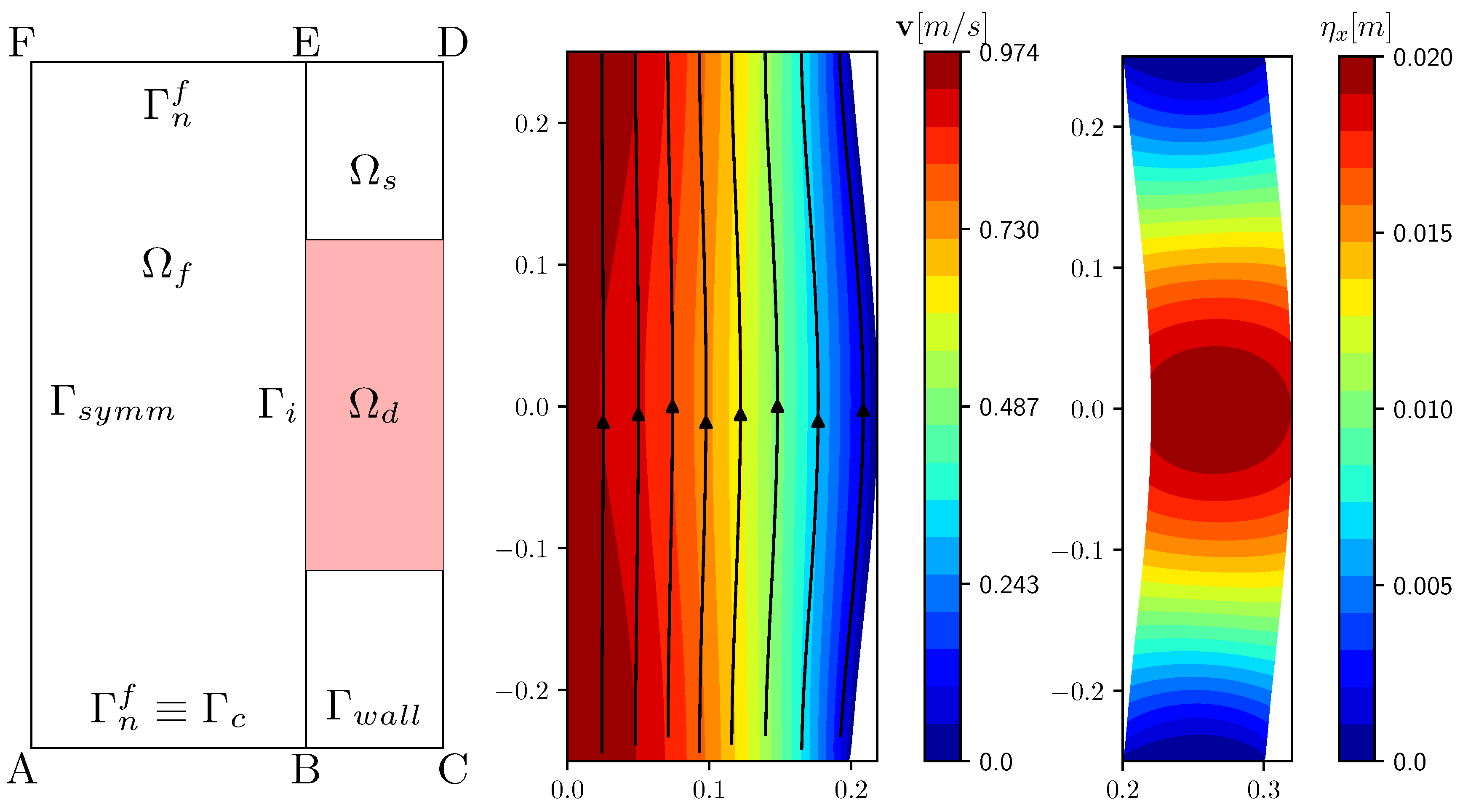
3.1. Test Case Configuration

In the first test case we consider a channel, shown in Figure 1 (on the left), where a fluid flows along the vertical direction. In order to simplify the computation, we consider a symmetric domain around the axis A F . The fluid inlet is defined by the segment AB and the outlet by EF. The domain consists of two rectangular regions ABEF and BCDE. The fluid flows in the rectangular region ABEF ( Ω f ) contained by the solid region BCDE ( Ω s ). The controlled domain is defined by Ω d . In this test we impose pressure boundary conditions with p E F = 10,000 Pa and p A B = 11,500 Pa. The segments AC and DF are fixed and the solid is free to move around the fixed endpoints C and D. We consider the physical properties as
ρ s = ρ f = 10 3 kg / m 3 , ν f = 0.07 m 2 / s , ν s = 0.2 , E = 10 6 Pa ,
so the solid can easily bend and the flow is not turbulent. This simple test case is used to compare the different optimal control approaches previously described by fixing the boundary conditions, physical properties and objective functional, while changing the control parameter in order to perform a meaningful comparison. The optimal control problems search for the optimal parameters, until the x-component of the displacement over the region Ω d matches the uniform target value η d = 0.05 m. The displacement in the remaining part of the solid domain is not controlled and therefore can take any value, solution of the state system.
Now we present the results referring to the reference case. We use the notation α = for the case with no control. If one solves the problem taking α = , then the optimal solution gives a vanishing control, since every other control would result in a functional higher than in the reference case. A standard laminar velocity profile develops in the fluid domain Ω f and is reported with streamlines in the center of Figure 1. The solid displacement in the solid domain Ω s is shown on the right of the same Figure. The main deformation occurs around the middle point of the right boundary and the maximum value is η x = 0.02 m, lower than the target value η d .

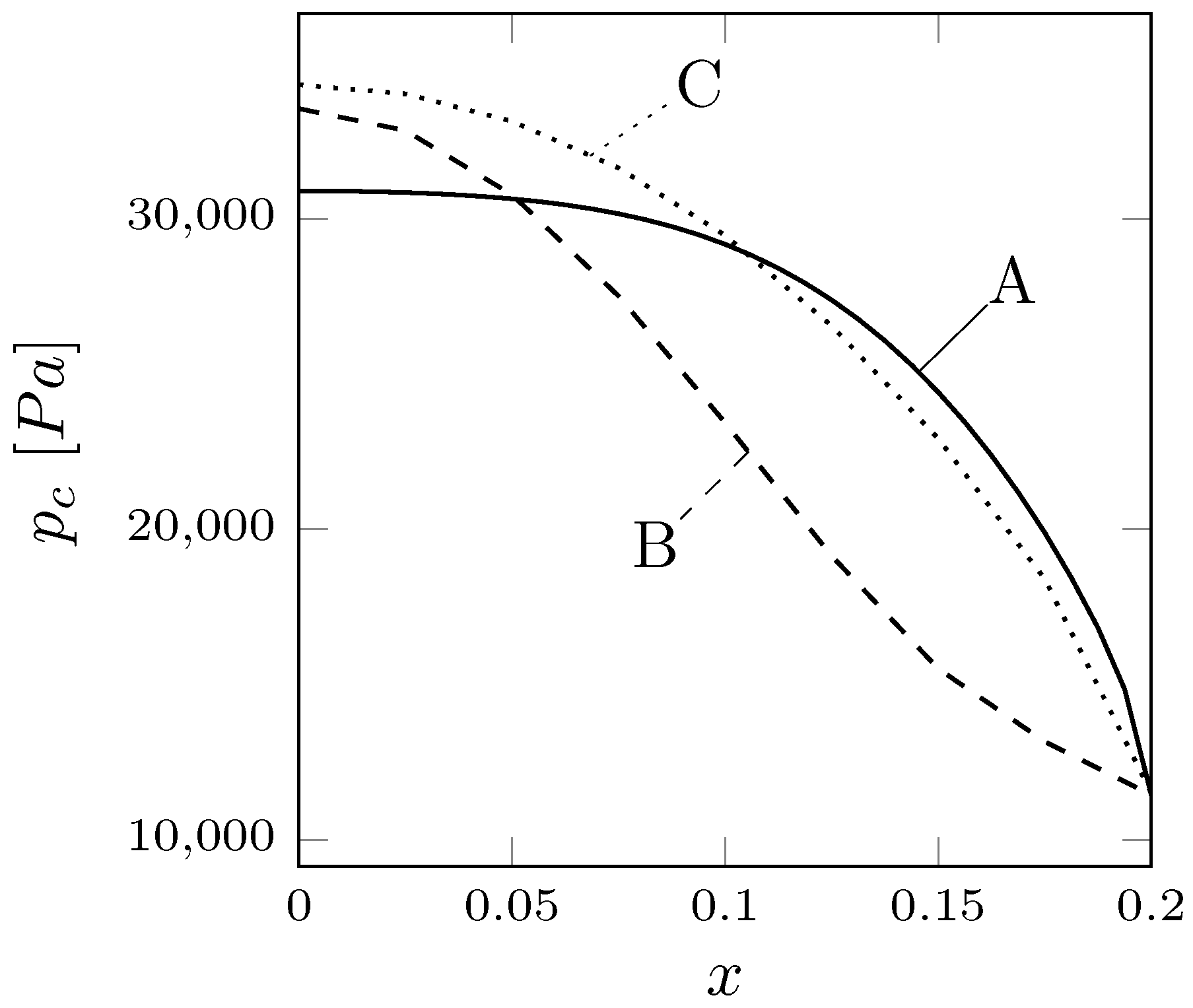
3.2. Pressure Boundary Control

The optimal control problem with optimal pressure on the lower fluid boundary Γ c minimizes the following functional
J ( η , p c ) = 1 2 Ω d ω ( η x 0.05 ) 2 d Ω + α 2 Γ c | p c | 2 d Γ .
We report in Table 1 the functional values J ( η , p ) and the mean values η ¯ x of the x-component of the displacement in the controlled region Ω d , obtained with different α values. By reducing α , the controlled solution tends to converge to the desired displacement and the functional values decrease. In Figure 2 a comparison is shown among the results obtained with different values of the regularization parameter α . The pressure profile over Γ c is reported as a function of the horizontal coordinate x for three values of the regularization parameter α = 10 8 , 10 9 and 10 10 . The pressure has a more uniform, regular profile as α decreases. In Figure 3 we report the results obtained when the optimal control problem is solved with α = 10 10 . On the left the fluid velocity with streamlines and, in the center, the solid displacement are shown. Due to the large pressure gradient between the fluid inlet and outlet the velocity is much higher than in the reference case. This may lead to convergence issues and eventually to a failure of the algorithm. Finally, on the right of the same figure, the adjoint velocity field is reported with streamlines at the beginning of the optimization algorithm.

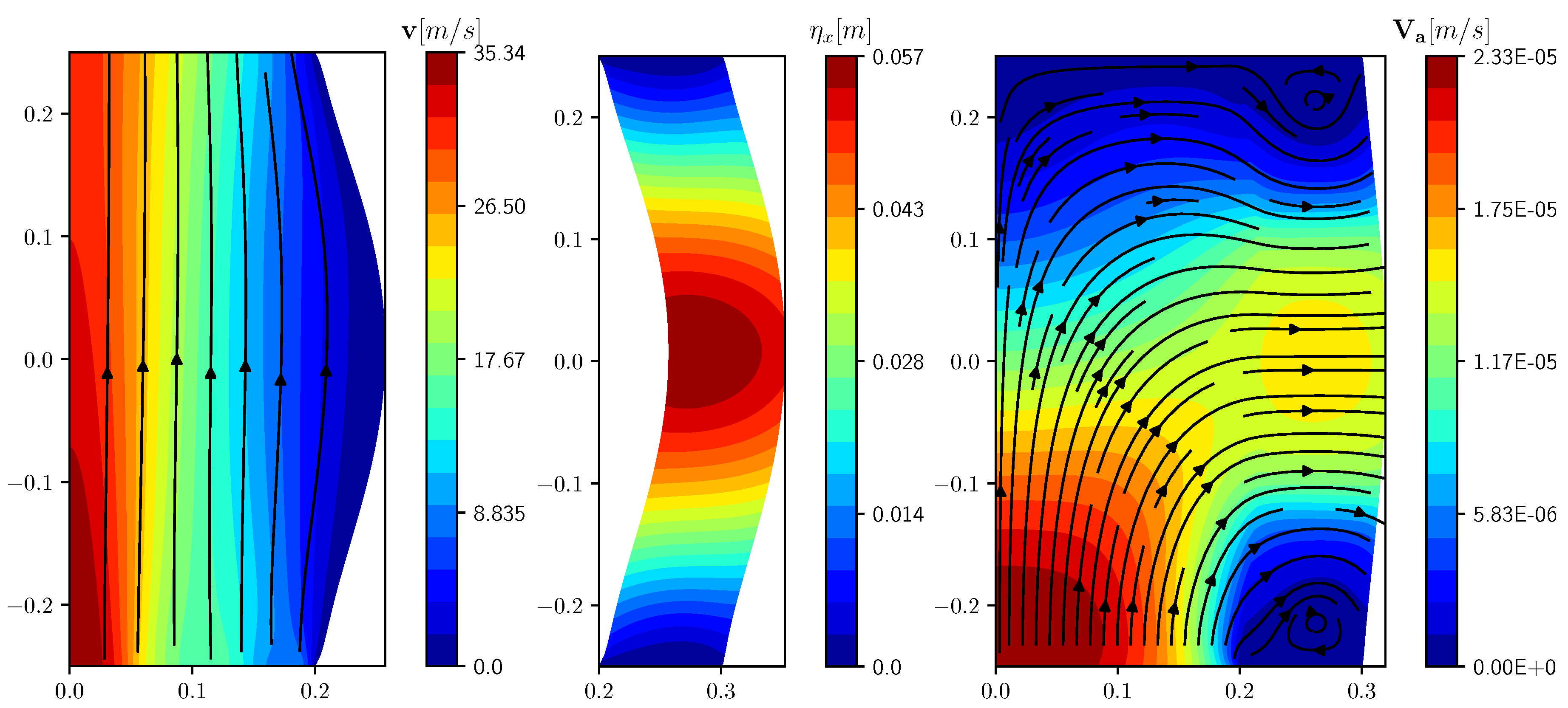
3.3. Distributed Control

Now we refer to the same solid displacement matching profile problem and focus on the distributed control case where the control is a force acting on the whole structure. This approach can be used in practical application to reformulate complex FSI shape optimization problems into simpler distributed control ones. The optimal control algorithm then aims to find the optimal force on the whole solid domain Ω s such that the x-component of the displacement over the region Ω d matches the uniform target value η d = 0.05 m. Therefore, the objective functional reads
J ( η , f ) = 1 2 Ω d ω ( η x 0.05 ) 2 d Ω + β 2 Ω c f 2 d Ω .
The results obtained in the controlled case with β = 10 13 are reported in Figure 4 and the functional J ( η , f ) , together with the mean horizontal displacement, in Table 2. Finally, we report, on the right of Figure 4, the profile of the force acting on the solid. The force has the highest intensity near the boundaries of the controlled domain Ω d and forces the solid mainly to the right. In the interior of Ω d the force is applied with lower intensity to the left in order to balance the stress induced on the controlled region by the fluid, obtaining a flat profile with uniform displacement.
We now compare these results with those obtained applying the pressure boundary control as shown in Section 3.2. We first notice that with the distributed control the fluid velocity in the optimized configuration is much lower. In fact, with the boundary control we have a large pressure gradient between the fluid inlet and outlet with the purpose to increase the velocity field. Now, on the contrary, the boundary pressure values are fixed and are the same as in the reference configuration with no control. The slightly different velocity profile is due to the obtained different solid configuration. Furthermore, the solid deformation is more uniform with an average value closer to the target one. The functional values reported in Table 2 are lower than those obtained with the boundary control, meaning that the distributed control has found an optimized solution closer to the desired one. One can see that the greatest improvements are obtained with the lowest regularization in both cases.

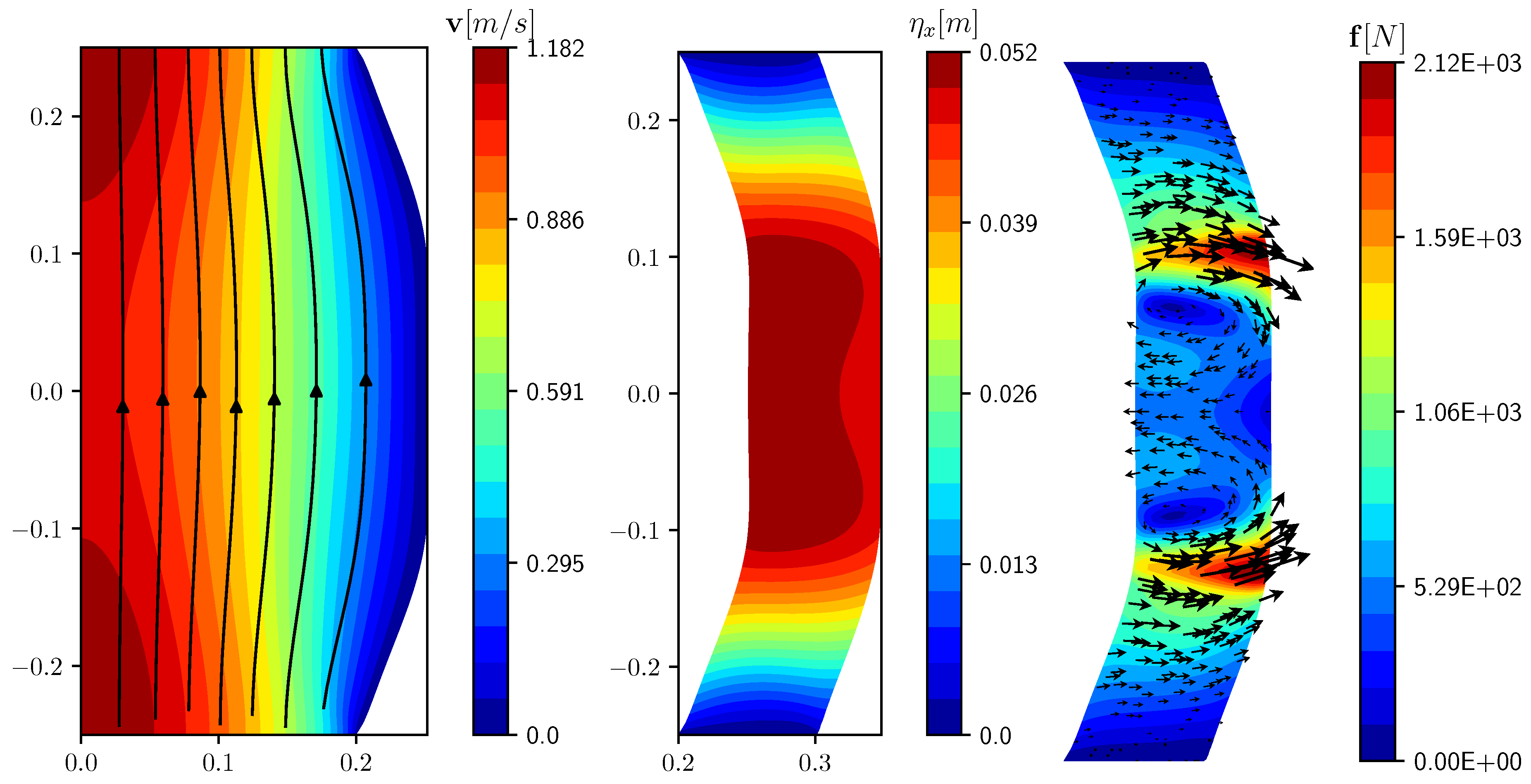
3.4. Parameter Estimation Problem

Our last optimal control approach aims to reach the solid target displacement η d by finding the optimal value of the Young modulus in Ω s . This problem has many industrially relevant applications, since changes in the mechanical properties as a function of temperature are commonly visible. The target displacement η x = 0.05 m in the region Ω d can be obtained only if the Young modulus is not uniform in the whole solid domain, with a complex distribution. The value of the Young modulus used for the reference case may be used as initial guess for the optimizing algorithm.
We use a multigrid approach for the solution of both the state and adjoint systems. The coarsest grid l = 0 has n e = 8 quadratic elements and the finer levels are obtained through a standard mid-point refinement approach. We solve the optimal control problem with different discretization levels, the finest one l = 5 has n e = 2048 elements (8385 grid nodes).
In Figure 5 we report the profile of the Young modulus E obtained after the optimization process, for l = 2 and with different values of the Young modulus lower bound E m i n . In order to improve the readability of the Figures we scaled all E values by 2.4 · 10 3 .
By comparing these results with the reference solution we notice that the control is able to obtain a profile close to the desired one. The Young modulus highest values are located near the middle point of the right side, which is the target region Ω d , in order to try to recover the desired uniform displacement. In the upper and lower parts of the solid sub-domain the solution is almost symmetric. By increasing the Young modulus lower limit the region near the solid endpoints where E = E m i n becomes larger, as well as the maximum value of E in the central region.
In Figure 6 we report the results obtained on the finest grid, l = 5 , with the same values of E m i n . By comparing these results with those obtained on a coarser grid (Figure 5), it is worth noticing that the solution is similar. Clearly, in the case l = 5 , the number of degrees of freedom available for the optimal control is higher and then, with higher resolution, the solid deformation is closer to the desired one, see Table 3. In this Table we report the functional obtained with different grid resolution, from l = 2 to l = 5 and with different values of the Young modulus lower bound E m i n . The effects of the penalty constraints are more important with higher lower bounds and the corresponding solutions are further away from the target one, in particular when E m i n = 200 Pa. We would like to point out that the functional value obtained with E m i n = 50 Pa is lower than this with E m i n = 10 Pa. Although it may seem strange, we recall that in the context of gradient-based optimization the final solution attained is usually affected by the choice of the initial guess and by the evolution of the solution during the optimization process. When E m i n 100 Pa the functionals are of the same order of magnitude as in the distributed control case and lower than those referring to the boundary control. Finally, the Young modulus profile, obtained with different values of E m i n , on the solid mid-line and on the fluid-solid interface is shown in Figure 7.

Control with Gradient Regularization

In this test, case we want to recover smoother E profiles, so we impose further regularization based on the gradient of the control. For this case we refer to the (20), take λ > 0 so that E H 1 ( Ω s ) and investigate the effects of the choice of λ .
In Figure 8, the Young modulus profile is shown for λ = 10 1 and 10 3 with E m i n = 10 Pa. In Table 4 we report the functional values obtained by changing the lower bound E m i n and with the same values of λ . The regularization term produces smoother solutions in particular with higher values of λ . In this case we have an optimal solution where the limits on the control are inactive and the control is not very effective. This can be deduced also from the plot on the right of the same Figure, where the Young modulus profile on the solid vertical mid-line is reported and has an almost uniform value in the whole domain. With λ = 10 1 , we obtain the same functional values for different E m i n which means that the inequality constraint is inactive. By taking λ = 10 3 , the regularization term becomes less important and the optimal solution recovered by the algorithm is closer to the target and to the one obtained with E L 2 ( Ω s ) , see Figure 7.

4. Conclusions

In this work, we have applied the optimal control theory to stationary fluid–structure interaction systems with the aim of keeping a single framework with different types of controls such as pressure, force, intensity and gradient of the Young modulus. The steady optimal problem has been reformulated by using a “fictitious” velocity field to obtain a symmetric adjoint system, coupling adjoint variables and forces on the interface, thus allowing us to use the same coupled solver for the state and adjoint systems. To solve the minimization problem we have adopted the Lagrangian multiplier method and the optimality system have been recovered by imposing the first-order necessary conditions. The objective of the optimal control problem is the matching of the desired displacement field in a particular region of the solid domain. This optimality system has been solved with an iterative gradient-based algorithm implemented in the FEM code.
We have studied and compared all the three optimization strategies: distributed, boundary and property controls. Distributed controls are the strongest ones while boundary controls are the weakest ones. As expected, the distributed control can act directly in the solid controlled region, with greater effectiveness. The effects of the boundary control instead have to propagate from the fluid boundary to the target domain that may be far away, which means that, in this case, the objective functional is less sensitive to the control parameter. The results obtained show the feasibility, the robustness and the weakness of the approaches proposed.

Author Contributions

Formal analysis, L.C. and S.M.; Investigation, L.C. and S.M.; Software, L.C. and S.M.; Validation, L.C. and S.M.; Writing–original draft, L.C. and S.M.; Writing–review & editing, L.C. All authors have read and agreed to the published version of the manuscript.

Funding

This research received no external funding.

Conflicts of Interest

The authors declare no conflict of interest.

References

  1. Gunzburger, M.D. Perspectives in Flow Control and Optimization; Siam: Philadelphia, PA, USA, 2003; Volume 5. [Google Scholar]
  2. Maute, K.; Nikbay, M.; Farhat, C. Sensitivity analysis and design optimization of three-dimensional non-linear aeroelastic systems by the adjoint method. Int. J. Numer. Methods. Eng. 2003, 56, 911–933. [Google Scholar] [CrossRef]
  3. Lund, E.; Møller, H.; Jakobsen, L.A. Shape design optimization of stationary fluid–structure interaction problems with large displacements and turbulence. Struct. Multidiscipl. Optim. 2003, 25, 383–392. [Google Scholar] [CrossRef]
  4. Bazilevs, Y.; Takizawa, K.; Tezduyar, T. Computational Fluid-Structure Interaction; John Wiley & Sons: Hoboken, NJ, USA, 2013. [Google Scholar]
  5. Bungartz, H.J.; Schäfer, M. Fluid-Structure Interaction: Modelling, Simulation, Optimisation; Springer Science & Business Media: Berlin/Heidelberg, Germany, 2006; Volume 53. [Google Scholar]
  6. Bodnár, T.; Galdi, G.P.; Nečasová, Š. Fluid-Structure Interaction and Biomedical Applications; Springer: Berlin/Heidelberg, Germany, 2014. [Google Scholar]
  7. Formaggia, L.; Quarteroni, A.; Veneziani, A. Cardiovascular Mathematics: Modeling and Simulation of the Circulatory System; Springer Science & Business Media: Berlin/Heidelberg, Germany, 2010; Volume 1. [Google Scholar]
  8. Degroote, J.; Bathe, K.J.; Vierendeels, J. Performance of a new partitioned procedure versus a monolithic procedure in fluid—Structure interaction. Comput. Struct. 2009, 87, 793–801. [Google Scholar] [CrossRef] [Green Version]
  9. Habchi, C.; Russeil, S.; Bougeard, D.; Harion, J.L.; Lemenand, T.; Ghanem, A.; Della Valle, D.; Peerhossaini, H. Partitioned solver for strongly coupled fluid–structure interaction. Comput. Fluids 2013, 71, 306–319. [Google Scholar] [CrossRef] [Green Version]
  10. Nobile, F.; Vergara, C. Partitioned algorithms for fluid–structure interaction problems in haemodynamics. Milan J. Math. 2012, 80, 443–467. [Google Scholar] [CrossRef] [Green Version]
  11. Causin, P.; Gerbeau, J.F.; Nobile, F. Added-mass effect in the design of partitioned algorithms for fluid–structure problems. Comput. Methods Appl. Mech. Eng. 2005, 194, 4506–4527. [Google Scholar] [CrossRef] [Green Version]
  12. Brenner, S.; Scott, R. The Mathematical Theory of Finite Element Methods; Springer Science & Business Media: Berlin/Heidelberg, Germany, 2007; Volume 15. [Google Scholar]
  13. Bramble, J.H. Multigrid Methods; CRC Press: Boca Raton, FL, USA, 1993; Volume 294. [Google Scholar]
  14. Turek, S.; Hron, J.; Madlik, M.; Razzaq, M.; Wobker, H.; Acker, J.F. Numerical simulation and benchmarking of a monolithic multigrid solver for fluid–structure interaction problems with application to hemodynamics. In Fluid Structure Interaction II; Springer: Berlin/Heidelberg, Germany, 2011; pp. 193–220. [Google Scholar]
  15. Richter, T. A monolithic multigrid solver for 3d fluid–structure interaction problems. Siam J. 2011. [Google Scholar] [CrossRef]
  16. Aulisa, E.; Bnà, S.; Bornia, G. A monolithic ALE Newton–Krylov solver with multigrid-Richardson–Schwarz preconditioning for incompressible fluid–structure interaction. Comput. Fluids 2018, 174, 213–228. [Google Scholar] [CrossRef] [Green Version]
  17. Failer, L.; Richter, T. A parallel Newton multigrid framework for monolithic fluid–structure interactions. J. Sci. Comput. 2020, 82, 28. [Google Scholar] [CrossRef] [Green Version]
  18. Failer, L.; Meidner, D.; Vexler, B. Optimal Control of a Linear Unsteady Fluid–Structure Interaction Problem. J. Optim. Theory Appl. 2016, 170, 1–27. [Google Scholar] [CrossRef]
  19. Perego, M.; Veneziani, A.; Vergara, C. A variational approach for estimating the compliance of the cardiovascular tissue: An inverse fluid–structure interaction problem. SIAM J. Sci. Comput. 2011, 33, 1181–1211. [Google Scholar] [CrossRef]
  20. Wick, T.; Wollner, W. Optimization with nonstationary, nonlinear monolithic fluid–structure interaction. Int. J. Numer. Methods Eng. 2020. [Google Scholar] [CrossRef] [Green Version]
  21. Chirco, L.; Manservisi, S. An adjoint based pressure boundary optimal control approach for fluid–structure interaction problems. Comput. Fluids 2019, 182, 118–127. [Google Scholar] [CrossRef]
  22. Richter, T.; Wick, T. Optimal control and parameter estimation for stationary fluid–structure interaction problems. SIAM J. Sci. Comput. 2013, 35, B1085–B1104. [Google Scholar] [CrossRef]
  23. Bazilevs, Y.; Hsu, M.C.; Bement, M. Adjoint-based control of fluid–structure interaction for computational steering applications. Procedia Comput. Sci. 2013, 18, 1989–1998. [Google Scholar] [CrossRef] [Green Version]
  24. Hron, J.; Turek, S. A monolithic FEM/multigrid solver for an ALE formulation of fluid–structure interaction with applications in biomechanics. In Fluid-Structure Interaction; Springer: Berlin/Heidelberg, Germany, 2006; pp. 146–170. [Google Scholar]
  25. Chirco, L.; Da Vià, R.; Manservisi, S. An optimal control method for fluid structure interaction systems via adjoint boundary pressure. J. Phys. Conf. Ser. 2017, 923, 012026. [Google Scholar] [CrossRef] [Green Version]
  26. Anzengruber, S.W.; Ramlau, R. Morozov’s discrepancy principle for Tikhonov-type functionals with nonlinear operators. Inverse Probl. 2009, 26, 025001. [Google Scholar] [CrossRef] [Green Version]
  27. Manservisi, S. An optimal control approach to an inverse nonlinear elastic shell problem applied to car windscreen design. Comput. Meth. Appl. Mech. Eng. 2000, 189, 463–480. [Google Scholar] [CrossRef]
  28. Manservisi, S.; Gunzburger, M. Variational inequality formulation of an inverse elasticity problem. Appl. Numer. Math. 2000, 34, 99–126. [Google Scholar] [CrossRef]
  29. Sokolowski, J.; Zolesio, J.P. Introduction to shape optimization. In Introduction to Shape Optimization; Springer: Berlin/Heidelberg, Germany, 1992; pp. 5–12. [Google Scholar]
  30. Armijo, L. Minimization of functions having Lipschitz continuous first partial derivatives. Pacific J. Math. 1966, 16, 1–3. [Google Scholar] [CrossRef] [Green Version]
  31. FEMuS—Multigrid Finite Element Code. Available online: https://github.com/FemusPlatform/femus (accessed on 5 August 2020).
  32. Aulisa, E.; Manservisi, S.; Seshaiyer, P. A computational multilevel approach for solving 2D Navier–Stokes equations over non-matching grids. Comput. Meth. Appl. Mech. Eng. 2006, 195, 4604–4616. [Google Scholar] [CrossRef]
  33. Cerroni, D.; Manservisi, S.; Menghini, F. An improved monolithic multigrid Fluid- Structure Interaction solver with a new moving mesh technique. Int. J. Math. Model. Meth. Appl. Sci. 2015, 9, 227–234. [Google Scholar]
  34. Girault, V.; Raviart, P.A. Finite Element Methods for Navier-Stokes Equations: Theory and Algorithms; Springer Science & Business Media: Berlin/Heidelberg, Germany, 2012; Volume 5. [Google Scholar]
Figure 1. Geometry and controlled region defined by dotted square on the right Ω d (left). Reference case with velocity profiles and streamlines in the liquid (center). Solid displacement field η x for the same reference configuration (right).
Fluids 05 00144 g001
Figure 2. Control pressure profile with α = 10 8 (A), α = 10 9 (B) and α = 10 10 (C).
Fluids 05 00144 g002
Figure 3. Controlled case with velocity profiles v and streamlines in the liquid (left) and displacement η in the solid (center). Adjoint velocity v a field and streamlines for the reference case configuration (right).
Fluids 05 00144 g003
Figure 4. Controlled case with velocity profiles v and streamlines in the liquid (left) and displacement η in the solid (center). Force vectors f in black and magnitude in colors (right).
Fluids 05 00144 g004
Figure 5. Young modulus E fields, discretization l = 2 with different E m i n = 10 Pa (left), 50 Pa (center), 100 Pa (right). E and E m i n are scaled by 2.4 · 10 3 .
Fluids 05 00144 g005
Figure 6. Young modulus E fields, discretization l = 5 with different E m i n = 10 Pa (left), 50 Pa (center), 100 Pa (right). E and E m i n are scaled by 2.4 · 10 3 .
Fluids 05 00144 g006
Figure 7. Young modulus profile on the solid vertical mid-line (left) and on the interface Γ i (right), with different E m i n = 10 Pa (A), 50 Pa (B), 100 Pa (C). E and E m i n are scaled by 2.4 · 10 3 .
Fluids 05 00144 g007
Figure 8. Young modulus E fields, discretization l = 5 with E m i n = 10 Pa and λ = 10 1 (left), λ = 10 3 (middle). Young modulus profile on the solid vertical mid-line (right), with E m i n = 10 Pa and λ = 10 1 (A), λ = 10 3 (B). E and E m i n are scaled by 2.4 · 10 3 .
Fluids 05 00144 g008
Table 1. Objective functional. The reference case with no control is labeled with α = .
α J ( η , p ) η ¯ x [ m ]
1.292 · 10 5 0.0180
10 8 9.192 · 10 6 0.0202
10 9 1.515 · 10 6 0.0469
10 10 6.454 · 10 7 0.0497
Table 2. Objective functional J and average x-displacement over the controlled region Ω d computed with no control ( β = ) and different β values.
β 10 11 10 12 10 13
J ( η , f ) · 10 8 1292.425.8545.88642.3875
η ¯ x [ m ] 0.01800.04940.04980.0499
Table 3. Objective functional. E m i n is scaled by 2.4 · 10 3 . The reference case with no control is labeled with NC.
E min [ Pa ]
Level1050100200NC
21.63 · 10 7 2.08 · 10 7 1.82 · 10 7 2.73 · 10 6 1.23 · 10 5
31.41 · 10 7 1.12 · 10 7 1.53 · 10 7 2.58 · 10 6 1.23 · 10 5
41.23 · 10 7 1.62 · 10 7 1.18 · 10 7 2.58 · 10 6 1.23 · 10 5
51.19 · 10 7 9.17 · 10 8 1.16 · 10 7 2.52 · 10 6 1.23 · 10 5
Table 4. Objective functionals. E m i n is scaled by 2.4 · 10 3 . The reference case with no control is labeled with NC.
E min [ Pa ]
λ 1050100200NC
10 1 3.29 · 10 7 3.29 · 10 7 3.51 · 10 7 2.68 · 10 6 1.23 · 10 5
10 3 9.79 · 10 8 9.20 · 10 8 3.22 · 10 7 2.68 · 10 6 1.23 · 10 5

