Stability of the Plane Bingham–Poiseuille Flow in an Inclined Channel

Abstract

We study the stability of laminar Bingham–Poiseuille flows in a sheet of fluid (open channel) down an incline with constant slope angle $\beta \in (0,\pi /2)$. This problem has geophysical applications to the evolution of landslides. In this article, we apply to this problem recent results of Falsaperla et al. for laminar Couette and Poiseuille flows of Newtonian fluids in inclined channels. The stability of the basic motion of the generalised Navier–Stokes system for a Bingham fluid in a horizontal channel against linear perturbations has been studied. In this article, we study the flows of a Bingham fluid when the channel is oblique and we prove a stabilizing effect of the Bingham parameter B. We also study the stability of the linear system with an energy method (Lyapunov functions) and prove that the streamwise perturbations are always stable, while the spanwise perturbations are energy-stable if the Reynolds number $\mathrm{Re}$ is less than the critical Reynolds number $R_c$ obtained solving a generalised Orr equation of a maximum variational problem.

1. Introduction

The stability of laminar flows in an inclined channel is important in many geophysical and industrial applications. Recently, Falsaperla et al. [1,2] described the stability of laminar flows of the steady solutions of a sheet of a Newtonian fluid (open channel) both in the horizontal case [1], and down an incline with constant slope angle $\beta$ [2]. In a reference frame $O, \mathbf{i}, \mathbf{j}, \mathbf{k}$ with $\mathbf{i}$ parallel to the incline and $\mathbf{k}$ orthogonal to the plane of the channel, let z be the coordinate of the axis orthogonal to the incline, the basic steady motion is given by the velocity field $U\left(z\right)\mathbf{i}$ and the pressure $p\left(z\right)$. For a laminar Newtonian fluid in a horizontal layer, $U\left(z\right)$ is linear for Couette flows and parabolic for Poiseuille flows, while, for an inclined channel, $U\left(z\right)$ is a parabolic function which vanishes at the bottom of the channel and whose derivative with respect to z vanish at the top.

Choosing an appropriately weighted $L_2$-energy equivalent to the classical energy norm, we prove in [1] that the plane Couette and Poiseuille flows are nonlinearly stable with respect to streamwise perturbations for any Reynolds number (see also [3]). We also prove in [4] that the plane Couette and Poiseuille flows are nonlinearly stable (and linearly stable in the energy norm) if the Reynolds number is less then the critical value

$${\mathrm{Re}}_{Orr}/sin\phi ,$$

when the perturbation is a tilted perturbation in the $x^{\prime }$ direction, with $x^{\prime }$ a coordinate associated to a new reference frame with ${\mathbf{i}}^{\prime }=\mathbf{i}cos\phi +\mathbf{j}sin\phi$, ${\mathbf{j}}^{\prime }=\mathbf{j}cos\phi -\mathbf{i}sin\phi$, and ${\mathbf{k}}^{\prime }=\mathbf{k}$. The number ${\mathrm{Re}}_{Orr}$ is the Orr [5] critical Reynolds number for spanwise perturbations which, for the Couette flow, is ${\mathrm{Re}}_{Orr}=177.22$ and for the Poiseuille flow is ${\mathrm{Re}}_{Orr}=175.31$. The results in [1] improve those obtained by Joseph [6], who found for streamwise perturbations a critical nonlinear value of $82.6$ in the plane Couette case, and those obtained by Joseph and Carmi [7], who found the value $99.1$ for plane Poiseuille flow for streamwise perturbations. The results we obtained in [1] are in a good agreement with the experiments and the numerical simulations. In a recent paper [2], we studied the stability of laminar Poiseuille flows for a Newtonian fluid in an oblique channel. That work is a preliminary investigation to model debris flows down an incline, and this work is its natural application to fluids which model those of realistic mudflows.

De Blasio, in his monograph, “Introduction to the Physics of Landslides” [8] introduces, in Chapter 4, non-Newtonian fluids, mudflows, and debris flows. In particular, he considers the behaviour of a mudflow described by Bingham rheology. He gives a first example of non-Newtonian fluid flow pattern considering a laminar stationary flow of a mud layer of thickness D along an inclined plane of infinite length [8] (pp. 100–103). He obtains the basic motion, but he does not investigate its stability. Basic flows of Bingham type in inclined channels arise also in other settings, for instance lubrication flows [9,10].

Bingham fluids are typically applied to drilling muds. They are subjected to a yield stress in addition to a plastic viscosity. The rheological properties are well-presented in the introduction of the paper by Frigaard et al. [11]. The stability (both in the linear and nonlinear case) of the horizontal laminar Poiseuille flows of a Bingham fluid has been investigated during the last 15 years by C. Nouar, I.A. Frigaard and co-workers [11,12,13,14,15,16]. In [12] the authors write: “Parallel duct flows of slurries and suspensions are relatively common in the petroleum and mining industries, where prediction of the flowregime can be an important design parameter in hydraulic systems. These complex fluids are commonly visco-plastic, meaning that they are characterised rheologically by having a yield stress, below which no deformation takes place”. Among other results, in [11,12,13,14,15,16], the plug (unyielded) zone and the yielded zone are introduced, and it is observed that the basic motion is the Bingham–Poiseuille flow, with basic velocity field $U\left(z\right)$ parabolic in the yielded zone and constant in the plug zone. In [14] the authors determine the yield surface and write the perturbation equations to the basic motion. They also linearise around the basic motion, and analyse the long-time behaviour of the disturbance which is transformed in an eigenvalue problem. They finally solve the eigenvalue problem with the appropriate boundary conditions using a Chebyshev collocation method, and investigate the dependence of the Reynods number on the Bingham parameter. In particular, they obtain the linear stability of the basic motion and prove that the Bingham number has a stabilizing effect.

The main aim of this work is to study the stability of the basic motion of the Bingham fluid down an inclined open channel as given in De Blasio, [8]. In particular, we study the stability of the linearised system of perturbations, and generalise to Bingham flows the stability results obtained for Newtonian fluids in [2]. Precisely, we prove that the basic motion is linearly stable for any Reynolds number and we prove (as in [11,12,13,14,15,16]) a stabilizing effect of the Bingham parameter. We also consider the linear stability studying the evolution in time of the energy of the perturbations, which amounts of investigating the stability in the energy norm with the Lyapunov method introduced by Reynolds [4] and Orr [5]. We prove that the streamwise perturbations are always stable while the spanwise perturbations are energy-stable if the Reynolds number $\mathrm{Re}$ is less than a critical Reynolds number $R_c$ obtained by solving a generalised Orr equation of a maximum variational problem.

We also observe that Allouche et al. [17] focussed on Newtonian and generalised Newtonian (in particular, Carreau) fluid film flows down an incline and compared the thresholds of oblique waves to those of two-dimensional waves for a given slope in order to reach the dominant instability in a given flow configuration. In particular they consider the shear-thinning and the shear-thickening cases and performed a temporal linear stability study on the problem. However, they do not study the stability of Bingham fluids.

In this article, we consider the stability in the linear context (both numerically and in energy). In a future paper we plan to investigate the nonlinear stability of Bingham flows and the stability of flows that obey to the Herschel–Bulkley rheology, which is even more appropriate in applications to landslides. We also plan to investigate, as in [1], the stability with respect to oblique perturbations and its relation with the experiments.

The layout of the paper is the following. In Section 2, following [8], we introduce the governing equations for a laminar open flow of a Bingham fluid down an inclined channel. In Section 3, following [11,12,13,14,15,16], we write the linearised equations for a perturbation to the basic motion $U\left(z\right)$ with the appropriate boundary conditions, and we solve the generalised Sommerfeld equations for the eigenvalue problem with the Chebyshev collocation method. In Section 4 we study the stability of the linearised perturbations with the Lyapunov method by using an energy norm, we find sufficient conditions for stability in energy for the streamwise and the spanwise perturbations and, for the latter, we write the Euler–Lagrange equations for the maximum problem and we solve the related generalised Orr equation. In Section 5, we draw some conclusions.

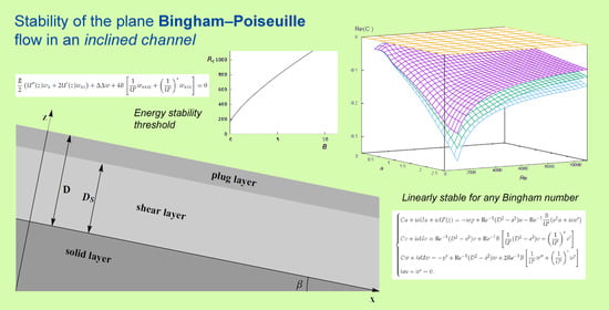
2. Laminar Open Flow of a Bingham Fluid Down an Inclined Channel

Consider the stationary laminar motion of a mud layer of thickness D along an inclined plane of infinite length with constant slope angle $\beta$, $0<\beta <\pi /2$ [8] (p. 100) in a reference frame $O, \mathbf{i}, \mathbf{j}, \mathbf{k}$ with associated coordinates $x,y,z$. The motion takes place in a channel ${\mathcal{D}}_1={\mathbb{R}}_{x,y}^2\times {[0,D]}_z$ of thickness D. The x-axis is taken along the slope direction while the z-axis is perpendicular to the slope. The y-axis is also parallel to the slope and orthogonal to the slope direction x. The channel extends indefinitely in the $x,y$ directions and has a finite depth D in the z direction (see Figure 1).

We consider the flow of an incompressible Bingham fluid with yield stress ${\tau }_0$ and plastic viscosity (Bingham viscosity) ${\mu }_B$. The wall placed in $z=0$ is rigid (the velocity of the flow vanishes) while that placed at $z=D$ is stress-free (the shear stress is zero). The governing equations are (cf. [11,12,13,14,15,16]):

$$\left\{\begin{array}{c}{\mathbf{U}}_t+\mathbf{U}·\nabla \mathbf{U}=\mathbf{g}-{\displaystyle \frac{1}{\rho }}\nabla \overline{p}+{\displaystyle \frac{1}{\rho }}\nabla ·\mathit{\tau }\left(\mathbf{U}\right),\hfill \\ \nabla ·\mathbf{U}=0,\hfill \end{array}\right.$$

where $\mathbf{U}$ is the velocity field, $\rho$ is the constant density, $\overline{p}$ is the pressure, $\mathit{\tau }$ is the deviatoric extra-stress tensor, ∇ is the gradient operator, and $\mathbf{g}$ is the gravity, $\mathbf{g}=gsin\beta \mathbf{i}-gcos\beta \mathbf{k}.$ The velocity vector is of the form $\mathbf{U}=U\mathbf{i}+V\mathbf{j}+W\mathbf{k}$, where U, V, W are the velocity components, and $\mathbf{i}$, $\mathbf{j}$, $\mathbf{k}$ are unit vectors in the streamwise (x) and spanwise (y) directions, and normal to the wall (z), respectively. As in [11,12,13,14,15,16], we assume the constitutive relations between the stress and the strain rate for a Bingham fluid

$$\left\{\begin{array}{c}\mathit{\tau }=\eta \dot{\gamma }\iff \tau \ge {\tau }_0\hfill \\ \dot{\gamma }=0\iff \tau <{\tau }_0,\hfill \end{array}\right.$$

(1)

where $\dot{\gamma }$ and $\mathit{\tau }$ are the strain rate and deviatoric stress tensors respectively. The yield stress is denoted by ${\tau }_0$ and $\eta$ denotes the effective viscosity, defined by

$$\eta ={\mu }_B+{\tau }_0{\dot{\gamma }}^{-1},$$

where ${\mu }_B$ is the Bingham viscosity (see De Blasio [8]), also called limiting viscosity (cf. [11]), ${\tau }_0$ is the yield stress, $\dot{\gamma }$ and $\tau$ are respectively the second invariants of the strain rate and the deviatoric stress tensors. They are given by $\dot{\gamma }=\sqrt{{\dot{\gamma }}_{ij}{\dot{\gamma }}_{ij}/2}$, $\tau =\sqrt{{\tau }_{ij}{\tau }_{ij}/2}$, ${\dot{\gamma }}_{ij}=U_{i,j}+U_{j,i}$, and the Einstein convention on summation of repeated indices has been assumed.

Following De Blasio [8], we assume that “the thickness of the mud flow does not change along the x coordinate, hence, U and $\overline{p}$ are independent of x”. So, we consider laminar shear flows $\mathbf{U}=U\left(z\right)\mathbf{i}$, $\overline{p}=\overline{p}\left(z\right)$ which are solutions to the stationary equations

$$\left\{\begin{array}{c}\mathbf{U}·\nabla \mathbf{U}=\mathbf{g}-{\displaystyle \frac{1}{\rho }}\nabla \overline{p}+{\displaystyle \frac{1}{\rho }}\nabla ·\mathit{\tau }\left(\mathbf{U}\right),\hfill \\ \nabla ·\mathbf{U}=0.\hfill \end{array}\right.$$

(2)

Equation (2) becomes

$$\left\{\begin{array}{c}gsin\beta +{\displaystyle \frac{1}{\rho }}{\displaystyle \frac{\partial {\tau }_{xz}}{\partial z}}=0\hfill \\ {\displaystyle \frac{1}{\rho }}{\displaystyle \frac{\partial \overline{p}}{\partial z}}+gcos\beta =0.\hfill \end{array}\right.$$

Solving these equations, we have

$$\left\{\begin{array}{c}{\tau }_{xz}=\rho gsin\beta z+\overline{A},\hfill \\ \overline{p}=-\rho gcos\beta z+\overline{B},\hfill \end{array}\right.$$

where $\overline{A}$ and $\overline{B}$ are integration constants that can be determined by imposing the chosen boundary conditions, that, in our case, are vanishing shear stress at the upper surface of the mud, i.e., ${\partial }_{z}U\left(D\right)=0$, and pressure equals to the atmospheric pressure $p_{atm}$. Applying Bingham Equation (1) and denoting $\tau ={\tau }_{xz}$, we have

$$\left\{\begin{array}{cc}{\mu }_B{\displaystyle \frac{\partial U}{\partial z}}=\tau -{\tau }_0=\rho gsin\beta (D-z)-{\tau }_0,\hfill & \mathrm{if}\tau \ge {\tau }_0,\hfill \\ {\displaystyle \frac{\partial U}{\partial z}}=0,\hfill & \mathrm{if}\tau \le {\tau }_0.\hfill \end{array}\right.$$

(3)

Following De Blasio [8] (p. 101), the first of two, Equation (3), can now be integrated from the base up to the level where the right-hand side becomes zero. This defines a layer known as the shear layer (the yielded zone) whose thickness $D_S$ can be found from Equation (3) imposing $\tau ={\tau }_0$. We find

$$z=D_S=D-{\displaystyle \frac{{\tau }_0}{\rho gsin\beta }}.$$

From Equation (3) and the definition of $D_S$ we have

$$\left\{\begin{array}{cc}{\mu }_B{\displaystyle \frac{\partial U}{\partial z}}=\tau -{\tau }_0=\rho gsin\beta (D-z)-{\tau }_0,\hfill & \mathrm{if}0\le z\le D_S\hfill \\ {\displaystyle \frac{\partial U}{\partial z}}=0,\hfill & \mathrm{if}z\ge D_S.\hfill \end{array}\right.$$

(4)

We note that for $z\le D_S$ the velocity $U\left(z\right)$ increases with height. For $z\ge D_S$, as De Blasio observes, the weight of the overlying material is not sufficient to shear the material, as it is obvious from the second of Equation (4). As a consequence, the material moves rigidly, $U\left(z\right)=c_0$ ($c_0$ a constant) like a plug. The thickness of this plug layer (unyielded zone) is

$$D_P=D-D_S={\displaystyle \frac{{\tau }_0}{\rho gsin\beta }}.$$

Integrating (4) and adopting the boundary conditions

$$U\left(0\right)=0,{\displaystyle \frac{\partial U\left(D_S\right)}{\partial z}}=0.$$

We have the basic Bingham-Poiesuille flow, $\overline{p}=p_{atm}+\rho gcos\beta (D-z)$, and

$$U\left(z\right)=\left\{\begin{array}{cc}{\displaystyle \frac{\rho gsin\beta }{{\mu }_B}}z\left[D_S-{\displaystyle \frac{z}{2}}\right]\hfill & \mathrm{if}0\le z\le D_S,\hfill \\ {\displaystyle \frac{\rho gsin\beta D_S^2}{2{\mu }_B}}\hfill & \mathrm{if}z\ge D_S,\hfill \end{array}\right.$$

These equations are non-dimensionalized using a length scale D, a velocity scale $U_0=U\left(D_S\right)=(\rho gsin\beta D_S^2)/\left(2{\mu }_B\right)$, and a pressure–stress scale $\rho U_0^2$. Introducing the non-dimensional Reynolds and Bingham numbers

$$\mathrm{Re}={\displaystyle \frac{\rho U_{0}D}{{\mu }_B}},B={\displaystyle \frac{{\tau }_{0}D}{{\mu }_B{U}_0}},$$

the non-dimensional form of (3) are

$$\left\{\begin{array}{cc}\tau ={\displaystyle \frac{1}{\mathrm{Re}}}\left({\displaystyle \frac{\partial U}{\partial z}}+B\right),\hfill & \mathrm{if}\tau \ge {\displaystyle \frac{B}{\mathrm{Re}}}\hfill \\ {\displaystyle \frac{\partial U}{\partial z}}=0,\hfill & \mathrm{if}\tau \le {\displaystyle \frac{B}{\mathrm{Re}}},\hfill \end{array}\right.$$

while the non-dimensional form of $U\left(z\right)$ is

$$U\left(z\right)=\left\{\begin{array}{c}1-{\displaystyle \frac{{(z-z_S)}^2}{z_S^2}},\mathrm{if}0\le z\le z_S,\hfill \\ 1,\mathrm{if}{z}_S\le z\le 1,\hfill \end{array}\right.$$

where $z_S=D_S/D$ is a positive number that represents the depth of the yield surface. Such depth can be computed directly, using the velocity $U_0$ and the Bingham number B, and solving the equation $B{z}_S^2=2(1-z_S)$, using the momentum conservation equation in the plug region, where we have ${\tau }_0=\left|{\tau }_w\right|$, with ${\tau }_w$ the wall shear stress $|{\tau }_w| = \tau (z=1)$ in the yielded region. In non-dimensional form, we have

$${\displaystyle \frac{B}{\mathrm{Re}(1-z_S)}}={\displaystyle \frac{1}{\mathrm{Re}}}{\left[{\displaystyle \frac{\partial U}{\partial z}}\right]}_{z=0}+{\displaystyle \frac{B}{\mathrm{Re}}}={\displaystyle \frac{B}{\mathrm{Re}}}\left[1+{\displaystyle \frac{2}{B{z}_S}}\right]\Rightarrow B={\displaystyle \frac{2(1-z_S)}{z_S^2}}\Rightarrow z_S={\displaystyle \frac{2}{1+\sqrt{1+2B}}}.$$

We observe that in the limit when B tends to 0, the fluid becomes a Newtonian fluid, and $z_S$ tends to 1. In such a limit case there is no plug region.

3. Linear Stability Analysis

In order to perform the linear stability analysis, as in [11,12,13,14,15,16], we introduce $(ϵ\mathbf{u},ϵp)$, infinitesimal perturbations to the basic flow $(U,\overline{p})$, with $ϵ<<1$ and $\left|\mathbf{u}\right|$ and p bounded. The linearised perturbation equation are

$$\left\{\begin{array}{c}ϵ{\mathbf{u}}_t+ϵ[\mathbf{u}·\nabla \mathbf{U}+\mathbf{U}·\nabla \mathbf{u}]=-ϵ\nabla p+\nabla ·[\mathit{\tau }(\mathbf{U}+ϵ\mathbf{u})-\mathit{\tau }\left(\mathbf{U}\right)],\hfill \\ \nabla ·\mathbf{u}=0.\hfill \end{array}\right.$$

(5)

wherever the yield stress is exceeded, the effective viscosity of the perturbed flow is expanded about the basic flow (see [14]). Denoting with $\mu$ the non dimensional effective viscosity, we have

$$\mu (\mathbf{U}\left(z\right)+ϵ\mathbf{u}(x,y,z,t))=\mu (U\left(z\right)+ϵu,ϵv,ϵw)={\displaystyle \frac{1}{\mathrm{Re}}}\left[1+{\displaystyle \frac{B}{\sqrt{A/2}}}\right],$$

(6)

where

$$A={\dot{\gamma }}_{ij}(\mathbf{U}+ϵ\mathbf{u}(x,y,z,t)){\dot{\gamma }}_{ij}(\mathbf{U}+ϵ\mathbf{u}(x,y,z,t)).$$

A simple calculation shows that

$$A=4{\left(ϵu_x\right)}^2+2{\left(ϵu_y+ϵv_x\right)}^2+2{\left({(U\left(z\right)+ϵu)}_z+ϵw_x)\right)}^2+4{\left(ϵv_y\right)}^2+2{(ϵv_z+ϵw_y)}^2+4{\left(ϵw_z\right)}^2,$$

(7)

where A depends on the number $ϵ$, $(u,v,w)$ are the components of $\mathbf{u}$, and the subscript indicate partial differentiation with respect to the variables. Expanding $\mu \left(\mathbf{U}\right(z)+ϵ\mathbf{u}(x,y,z,t\left)\right)$ in powers of $ϵ$, we have

$$\mu (\mathbf{U}\left(z\right)+ϵ\mathbf{u}(x,y,z,t))=\mu \left(\mathbf{U}\left(z\right)\right)+\frac{\partial }{\partial ϵ}\left(\mu \left(\mathbf{U}\right(z)+ϵ\mathbf{u}(x,y,z,t\left)\right)\right){|}_{ϵ=0}ϵ+O\left({ϵ}^2\right).$$

From (6) it follows that

$$\frac{\partial \mu }{\partial ϵ}{|}_{ϵ=0}=-\frac{B}{4\mathrm{Re}}\cdot \frac{1}{{(U\prime )}^2\left|U\prime \right|}\cdot \frac{\partial A}{\partial ϵ}{|}_{ϵ=0},$$

where $U^{\prime }$ is the derivative of U with respect to z. Finally, at the first order in $ϵ$ we have:

$$\mu (\mathbf{U}\left(z\right)+ϵ\mathbf{u}(x,y,z,t))={\displaystyle \frac{1}{\mathrm{Re}}}\left[1+{\displaystyle \frac{B}{|U^{\prime }|}}-{\displaystyle \frac{B}{|U^{\prime }|U^{\prime }}}(u_z+w_x)ϵ\right].$$

We recall that

$$\tau (\mathbf{U}+ϵ\mathbf{u})-\tau \left(\mathbf{U}\right)=\mu (\mathbf{U}+ϵ\mathbf{u})(\dot{\gamma }\left(\mathbf{U}\right)+ϵ\dot{\gamma }\left(\mathbf{u}\right))-\mu \left(\mathbf{U}\right)\dot{\gamma }\left(\mathbf{U}\right).$$

Computing $\dot{\gamma }\left(\mathbf{U}\right)$ and by observing that $U^{\prime }\ge 0$, at the first order in $ϵ$, we have

$$\mathit{\tau }(\mathbf{U}+ϵ\mathbf{u})-\mathit{\tau }\left(\mathbf{U}\right)=ϵ\left[{\displaystyle \frac{1}{\mathrm{Re}}}\left(1+{\displaystyle \frac{B}{U^{\prime }}}\right)\dot{\gamma }\left(\mathbf{u}\right)-(u_z+w_x){\displaystyle \frac{B}{\mathrm{Re}{\left(U^{\prime }\right)}^2}}\dot{\gamma }\left(\mathbf{U}\right)\right].$$

From this relation, we easily obtain

$${\displaystyle \frac{1}{ϵ}}{\left[\tau (\mathbf{U}+ϵ\mathbf{u})-\tau \left(\mathbf{U}\right)\right]}_{ij}={\beta }_{ij},$$

(8)

with

$${\beta }_{ij}=\left\{\begin{array}{cc}{\mathrm{Re}}^{-1}\left(1+{\displaystyle \frac{B}{U^{\prime }}}\right){\dot{\gamma }}_{ij}\left(\mathbf{u}\right)\hfill & \mathrm{if}(i,j)\ne (1,3)\mathrm{or}(3,1)\hfill \\ {\mathrm{Re}}^{-1}{\dot{\gamma }}_{ij}\left(\mathbf{u}\right)\hfill & \mathrm{if}(i,j)=(1,3)\mathrm{or}(3,1).\hfill \end{array}\right.$$

(9)

Collecting (5), (8) and (9), we have

$$\left\{\begin{array}{c}{\mathbf{u}}_t+\mathbf{u}·\nabla \mathbf{U}+\mathbf{U}·\nabla \mathbf{u}=-\nabla p+{\left({\beta }_{ij}\right)}_i{\mathbf{e}}_j\hfill \\ \nabla ·\mathbf{u}=0\hfill \end{array}\right.$$

(10)

where we have used the convention $1=x$, $2=y$, $3=z$ and ${\mathbf{e}}_1=\mathbf{i}$, ${\mathbf{e}}_2=\mathbf{j}$, ${\mathbf{e}}_3=\mathbf{k}$. The perturbation Equation (10) in the open domain ${\mathcal{D}}_S={\mathbb{R}}^2\times (0,z_S)$, written with respect to the components $(u,v,w)$ of $\mathbf{u}$, are

$$\left\{\begin{array}{c}{u}_t+w{U}^{\prime }+U{u}_x=-p_x+{\displaystyle \frac{1}{\mathrm{Re}}}\Delta u+{\displaystyle \frac{B}{\mathrm{Re}{U}^{\prime }}}(u_{xx}+u_{yy}-w_{xz}),\hfill \\ v_t+U{v}_x=-p_y+{\displaystyle \frac{1}{\mathrm{Re}}}\Delta v+{\displaystyle \frac{B}{\mathrm{Re}}}\left[{\displaystyle \frac{1}{U^{\prime }}}(v_{xx}+v_{yy}+v_{zz})+{\left({\displaystyle \frac{1}{U^{\prime }}}\right)}^{\prime }(v_z+w_y)\right],\hfill \\ w_t+U{w}_x=-p_z+{\displaystyle \frac{1}{\mathrm{Re}}}\Delta w+{\displaystyle \frac{B}{\mathrm{Re}}}\left[{\displaystyle \frac{1}{U^{\prime }}}(w_{yy}+w_{zz}+v_{yz}+w_{zz})+2{\left({\displaystyle \frac{1}{U^{\prime }}}\right)}^{\prime }{w}_z\right],\hfill \end{array}\right.$$

(11)

where $\Delta$ is the Laplacian. We assume that the perturbations $\mathbf{u},p$ are periodic in x and y of periods $2\pi /a$, $2\pi /b$, with wave number a and b in the directions x and y. We will later consider the limit cases of streamwise perturbations, i.e., perturbations which do not depend on x and are periodic only on y, and spanwise perturbations, i.e., perturbations which do not depend on y and are periodic only on x.

Equation (11) must be completed with a set of boundary conditions. Since, for a yield stress fluid $U^{\prime }=-2(z-z_S)/z_S^2$ and $1/U^{\prime }$ is singular as $z\to z_S$, the effective viscosity goes to $+\infty$ at the yield surface. It follows that some care is required in deriving the boundary conditions at $z=z_S$ as explained for example in [11,14]. As in [11], we assume that the yield surface $z=z_S$ is perturbed to $\widehat{z}=z_S+ϵh(x,y,t)$, with $h(x,y,t)$ periodic in x and y of periods $2\pi /a$, $2\pi /b$. The boundary conditions can be obtained as in [11,13,14,15,16] and turn out to be

$$\left\{\begin{array}{c}u(x,y,0,t)=v(x,y,0,t)=w(x,y,0,t)=0,\hfill \\ u(x,y,z_S,t)=v(x,y,z_S,t)=w(x,y,z_S,t)=0,\hfill \\ {\displaystyle \frac{\partial v(x,y,z_s,t)}{\partial z}}={\displaystyle \frac{\partial w(x,y,z_s,t)}{\partial z}}=0,{\displaystyle \frac{\partial u(x,y,z_s,t)}{\partial z}}=-h{U}^{″}\left(z_s\right).\hfill \end{array}\right.$$

The boundary conditions at $z=0$ are rigid, as classically found in Newtonian fluids. The Dirichlet boundary conditions $\mathbf{u}=0$ at the yield surface can be deduced from the fact that the unyielded plug zone is constrained to move as a rigid body according to the Bingham model [13]. The Neumann conditions come from linearisation of the condition ${\dot{\gamma }}_{ij}(\mathbf{U}+ϵ\mathbf{u})=0$ at the perturbed yield surface, onto the unperturbed yield surface position [13]. In particular, following [13], we note that the conditions ${\partial }_{z}v(x,y,z_s,t)={\partial }_{z}w(x,y,z_s,t)=0$, are necessary due to the singular behaviour of $1/U^{\prime }$ on $z=z_S$ in the non-Newtonian part of (11). These boundary conditions ensure that (11) are well-defined as $z\to z_S$. We thus have that v and w are asymptotic at $z_S$ to ${(z-z_S)}^{\alpha }$, with $\alpha >1$. This fact will be useful in the Lyapunov investigation, in particular when using the boundary conditions in the periodicity cell $\mathsf{\Omega }=[0,2\pi /a]\times [0,2\pi /b]\times [0,z_S]$.

In order to study the linear stability with the spectral method, we assume that the perturbations have the form

$$(u,v,w,p,h)=[u\left(z\right),v\left(z\right),w\left(z\right),p\left(z\right),h]e^{i(ax+by)+Ct},$$

where C is a complex number whose real part gives the decay rate of the perturbation.

We observe that, in [13], Frigaard and Nouar prove a Squire-like (see [18]) theorem: “if the equivalent eigenvalue bounds for a Newtonian fluid yield a stability criterion, then the same stability criterion is valid for the Bingham fluid flow, but with reduced wavenumbers and Reynolds numbers”. Assuming this, we consider in what follows only streamwise or only spanwise perturbations.

In the case of streamwise perturbations $a=0$ and $b\ne 0$, we hence have

$$\left\{\begin{array}{c}Cu+w{U}^{\prime }\left(z\right)={\mathrm{Re}}^{-1}(D^2-b^2)u-{\mathrm{Re}}^{-1}{\displaystyle \frac{B}{U^{\prime }}}{b}^{2}u\hfill \\ Cv=-ibp+{\mathrm{Re}}^{-1}(D^2-b^2)v+{\mathrm{Re}}^{-1}B\left[{\displaystyle \frac{1}{U^{\prime }}}(D^2-b^2)v+{\left({\displaystyle \frac{1}{U^{\prime }}}\right)}^{\prime }(v^{\prime }+ibw)\right]\hfill \\ Cw=-p^{\prime }+{\mathrm{Re}}^{-1}(D^2-b^2)w+{\mathrm{Re}}^{-1}B\left[{\displaystyle \frac{1}{U^{\prime }}}(-b^{2}w+2w^{″}+ib{v}^{\prime })+2{\left({\displaystyle \frac{1}{U^{\prime }}}\right)}^{\prime }{w}^{\prime }\right]\hfill \\ ibv+w^{\prime }=0.\hfill \end{array}\right.$$

An easy calculation proves that the streamwise perturbations are always stable (the real part of C is always less than 0). For the spanwise perturbations $a\ne 0$ and $b=0$, and we have

$$\left\{\begin{array}{c}Cu+iaUu+w{U}^{\prime }\left(z\right)=-iap+{\mathrm{Re}}^{-1}(D^2-a^2)u-{\mathrm{Re}}^{-1}{\displaystyle \frac{B}{U^{\prime }}}(a^{2}u+ia{w}^{\prime })\hfill \\ Cv+iaUv={\mathrm{Re}}^{-1}(D^2-a^2)v+{\mathrm{Re}}^{-1}B\left[{\displaystyle \frac{1}{U^{\prime }}}(D^2-a^2)v+{\left({\displaystyle \frac{1}{U^{\prime }}}\right)}^{\prime }{v}^{\prime }\right]\hfill \\ Cw+iaUw=-p^{\prime }+{\mathrm{Re}}^{-1}(D^2-a^2)w+2{\mathrm{Re}}^{-1}B\left[{\displaystyle \frac{1}{U^{\prime }}}{w}^{″}+{\left({\displaystyle \frac{1}{U^{\prime }}}\right)}^{\prime }{w}^{\prime }\right]\hfill \\ iau+w^{\prime }=0.\hfill \end{array}\right.$$

(12)

The variable v appears only in the second equation of system (12), and it can proven that v cannot destabilize the basic motion. The remaining three equations depend only on $u,w$ and on the pressure p. Using the continuity equation, one can further eliminate the variables $u,p$ and derive a system of one equation in the variable w. This can be obtained by subtracting $ia$ times the z-derivative of the first equation of (12) and adding the third equation of (12) multiplied by $a^2$ (this amounts to writing the equation of the third component of the doube-curl of $\mathbf{u}$). In this way one obtains the generalised Orr–Sommerfeld equation

$$(C+iaU)(w^{″}-a^{2}w)-iaw{U}^{″}\left(z\right)={\mathrm{Re}}^{-1}(w^{⁗}-2a^2{w}^{″}+a^{4}w)-4a^{2}B{\mathrm{Re}}^{-1}\left[{\displaystyle \frac{w^{″}}{U^{\prime }}}+{\left({\displaystyle \frac{1}{U^{\prime }}}\right)}^{\prime }{w}^{\prime }\right],$$

with boundary conditions

$$w(x,y,0)=w_z(x,y,0)=0,w(x,y,z_S)=w_z(x,y,z_S)=0.$$

Numerical calculations show that the linear perturbations are always stable, i.e., the real part of C is negative for any Reynolds number. The Chebyshev collocation method has been used up to 100 polynomials for w. This transforms the differential equation in an algebraic generalized eigenvalue system which also takes into account the given boundary conditions. Figure 2 shows that the maximum real part of the spectrum of C is negative and decreasing with the Bingham number. Here, we have considered the significative ranges $a\in [0,2.6]$, $\mathrm{Re}\in [1000,11000]$. We also obtain the expected fact that as $\mathrm{Re}$ tends to 0, the real part of C tends to $-\infty$.

4. Linear-Energy Stability of Perturbations

In this section we use the linear Lyapunov method, also typically called energy-stability method. In the periodicity cell $\mathsf{\Omega }$, we introduce the scalar product $(,)$ and the $L^2\left(\mathsf{\Omega }\right)$ norm $\parallel ·\parallel$. We have the energy identities:

$$\begin{array}{c}{\displaystyle \frac{d}{dt}}\left[{\displaystyle \frac{{\parallel u\parallel }^2}{2}}\right]+(w{U}^{\prime },u)+(U{u}_x,u)=-(p_x,u)+{\displaystyle \frac{1}{\mathrm{Re}}}(\Delta u,u)+{\displaystyle \frac{B}{\mathrm{Re}}}\left[\left({\displaystyle \frac{1}{U^{\prime }}}(u_{xx}+u_{yy}-w_{xz}),u\right)\right]\hfill \\ {\displaystyle \frac{d}{dt}}\left[{\displaystyle \frac{{\parallel v\parallel }^2}{2}}\right]+(U{v}_x,v)=-(p_y,v)+{\displaystyle \frac{1}{\mathrm{Re}}}(\Delta v,v)+{\displaystyle \frac{B}{\mathrm{Re}}}\left[\left({\displaystyle \frac{1}{U^{\prime }}}\Delta v,v\right)+\left({\left({\displaystyle \frac{1}{U^{\prime }}}\right)}^{\prime }(v_z+w_y),v\right)\right]\hfill \\ {\displaystyle \frac{d}{dt}}\left[{\displaystyle \frac{{\parallel w\parallel }^2}{2}}\right]+(U{w}_x,w)=-(p_z,w)+{\displaystyle \frac{1}{\mathrm{Re}}}(\Delta w,w)+{\displaystyle \frac{B}{\mathrm{Re}}}\left[\left({\displaystyle \frac{1}{U^{\prime }}}(w_{yy}+2w_{zz}+v_{yz})+{\left({\displaystyle \frac{2}{U^{\prime }}}\right)}^{\prime }{w}_z,w\right)\right].\hfill \end{array}$$

These identities can be simplified by applying integration by parts and using the boundary conditions. Since the term $(U{u}_x,u)$ integrates to zero

$$(U{u}_x,u)=\left(U,{\displaystyle \frac{\partial }{\partial x}}{\displaystyle \frac{u^2}{2}}\right)=\underset{\overline{z}\to z_S}{lim}{\left[U{\displaystyle \frac{u^2}{2}}\right]}_{z=0}^{\overline{z}}=0.$$

We have the simplified identities

$${\displaystyle \frac{d}{dt}}\left[{\displaystyle \frac{{\parallel u\parallel }^2}{2}}\right]+(w{U}^{\prime },u)=-(p_x,u)-{\displaystyle \frac{1}{\mathrm{Re}}}{\parallel \nabla u\parallel }^2+{\displaystyle \frac{B}{\mathrm{Re}}}\left[\left({\displaystyle \frac{1}{U^{\prime }}}(u_{xx}+u_{yy}-w_{xz}),u\right)\right]$$

(13)

$${\displaystyle \frac{d}{dt}}\left[{\displaystyle \frac{{\parallel v\parallel }^2}{2}}\right]=-(p_y,v)-{\displaystyle \frac{1}{\mathrm{Re}}}{\parallel \nabla v\parallel }^2+{\displaystyle \frac{B}{\mathrm{Re}}}\left[\left({\displaystyle \frac{1}{U^{\prime }}}\Delta v,v\right)+\left({\left({\displaystyle \frac{1}{U^{\prime }}}\right)}^{\prime }(v_z+w_y),v\right)\right]$$

(14)

$${\displaystyle \frac{d}{dt}}\left[{\displaystyle \frac{{\parallel w\parallel }^2}{2}}\right]=-(p_z,w)-{\displaystyle \frac{1}{\mathrm{Re}}}{\parallel \nabla w\parallel }^2+{\displaystyle \frac{B}{\mathrm{Re}}}\left[\left({\displaystyle \frac{1}{U^{\prime }}}(w_{yy}+2w_{zz}+v_{yz})+{\left({\displaystyle \frac{2}{U^{\prime }}}\right)}^{\prime }{w}_z,w\right)\right].$$

(15)

4.1. Stability of Streamwise Perturbations

To prove that the linear streamwise perturbations are always stable, we begin observing that, for streamwise perturbations, ${\partial }_x\equiv 0$. The solenoidality of the kinetic perturbation hence reads $v_y+w_z=0$. From (14) and (15), we have

$$\begin{array}{c}{\displaystyle \frac{1}{2}}{\displaystyle \frac{d}{dt}}\left[{\parallel v\parallel }^2+{\parallel w\parallel }^2\right]=-{\displaystyle \frac{1}{\mathrm{Re}}}{(\parallel \nabla v\parallel }^2+{\parallel \nabla w\parallel }^2)\hfill \\ +{\displaystyle \frac{B}{\mathrm{Re}}}\left[\left({\displaystyle \frac{1}{U^{\prime }}}\Delta v,v\right)+\left({\left({\displaystyle \frac{1}{U^{\prime }}}\right)}^{\prime }(v_z+w_y),v\right)\right]+{\displaystyle \frac{B}{\mathrm{Re}}}\left({\displaystyle \frac{1}{U^{\prime }}}(w_{yy}+w_{zz})+{\left({\displaystyle \frac{2}{U^{\prime }}}\right)}^{\prime }{w}_z,w\right).\hfill \end{array}$$

(16)

From (16), we have

$$\begin{array}{cc}\hfill \left({\displaystyle \frac{1}{U^{\prime }}}\Delta v,v\right)& =\left({\displaystyle \frac{1}{U^{\prime }}}(v_{yy}+v_{zz}),v\right)=\hfill \\ & =-\left({\displaystyle \frac{1}{U^{\prime }}}{v}_y,v_y\right)+\underset{\overline{z}\to z_S}{lim}{\left[{\displaystyle \frac{1}{U^{\prime }}}{v}_{z}v\right]}_{z=0}^{\overline{z}}-\left({\left({\displaystyle \frac{1}{U^{\prime }}}\right)}^{\prime }{v}_z,v\right)-\left({\displaystyle \frac{1}{U^{\prime }}}{v}_z,v_z\right)\hfill \\ & =-{\int }_{\mathsf{\Omega }}{\displaystyle \frac{v_y^2+v_z^2}{U^{\prime }}}d\mathsf{\Omega }-{\int }_{\mathsf{\Omega }}{\left({\displaystyle \frac{1}{U^{\prime }}}\right)}^{\prime }{\displaystyle \frac{\partial }{\partial z}}\left({\displaystyle \frac{v^2}{2}}\right)d\mathsf{\Omega }\hfill \\ & =-{\int }_{\mathsf{\Omega }}{\displaystyle \frac{v_y^2+v_z^2}{U^{\prime }}}d\mathsf{\Omega }-\underset{\overline{z}\to z_S}{lim}{\left[{\left({\displaystyle \frac{1}{U^{\prime }}}\right)}^{\prime }{\displaystyle \frac{v^2}{2}}\right]}_{z=0}^{\overline{z}}+{\int }_{\mathsf{\Omega }}{\left({\displaystyle \frac{1}{U^{\prime }}}\right)}^{″}{\displaystyle \frac{v^2}{2}}d\mathsf{\Omega }.\hfill \end{array}$$

We observe that as $\overline{z}\to z_S$ we have

$${\displaystyle \frac{1}{U^{\prime }}}v\simeq {(\overline{z}-z_S)}^{\alpha -1},\mathrm{and}{\left({\displaystyle \frac{1}{U^{\prime }}}\right)}^{\prime }{v}^2\simeq {(\overline{z}-z_S)}^{2(\alpha -1)}.$$

Hence, the boundary terms vanish. Proceeding in the same way for the other terms, we easily obtain:

$$\begin{array}{c}{\displaystyle \frac{1}{2}}{\displaystyle \frac{d}{dt}}\left[{\parallel v\parallel }^2+{\parallel w\parallel }^2\right]\hfill \\ =-{\displaystyle \frac{1}{\mathrm{Re}}}{(\parallel \nabla v\parallel }^2+{\parallel \nabla w\parallel }^2)-{\displaystyle \frac{B}{\mathrm{Re}}}\left[{\int }_{\mathsf{\Omega }}{\displaystyle \frac{1}{U^{\prime }}}(v_y^2+w_y^2+v_z^2+w_z^2)d\mathsf{\Omega }+{\int }_{\mathsf{\Omega }}{\left({\displaystyle \frac{1}{U^{\prime }}}\right)}^{″}{w}^{2}d\mathsf{\Omega }\right].\hfill \end{array}$$

Since

$${\displaystyle \frac{1}{U^{\prime }}}=-{\displaystyle \frac{z_s^2}{2(z-z_S)}}>0\mathrm{and}{\left({\displaystyle \frac{1}{U^{\prime }}}\right)}^{″}=-{\displaystyle \frac{z_S^2}{{(z-z_S)}^3}}>0\mathrm{in}0<z<z_S,$$

Poincaré inequality allows us to prove that $\parallel v\parallel$ and $\parallel w\parallel$ decay exponentially to 0 as $t\to +\infty$. By using (13), it easy to see that also $\parallel u\parallel$ goes to 0 as $t\to +\infty$. Therefore, the energy norm of the kinetic perturbation tends to 0 for any Reynolds and Bingham number. We conclude that the streamwise perturbations are always linearly stabilizing.

4.2. Stability of Spanwise Perturbations

To investigate the spanwise perturbations we begin observing that, in this case, ${\partial }_y\equiv 0$. It follows that the solenoidality of the kinetic perturbation reads $u_x+w_z=0$. From (14), integrating by parts, and using the boundary conditions as before, we have:

$$\begin{array}{cc}\hfill {\displaystyle \frac{d}{dt}}\left[{\displaystyle \frac{{\parallel v\parallel }^2}{2}}\right]& =-{\mathrm{Re}}^{-1}{\parallel \nabla v\parallel }^2+{\mathrm{Re}}^{-1}B\left[\left({\displaystyle \frac{1}{U^{\prime }}}\Delta v,v\right)+\left({\left({\displaystyle \frac{1}{U^{\prime }}}\right)}^{\prime }{v}_z,v\right)\right]\hfill \\ & =-{\mathrm{Re}}^{-1}{\parallel \nabla v\parallel }^2-{\mathrm{Re}}^{-1}B{\int }_{\mathsf{\Omega }}{\displaystyle \frac{1}{U^{\prime }}}(v_x^2+v_z^2)d\mathsf{\Omega }.\hfill \end{array}$$

Applying the Poincaré inequality and observing that $1/U^{\prime }=-z_s^2/\left(2(z-z_S)\right)>0$ for $z<z_S$, we have that $\parallel v\parallel$ goes exponentially to 0 as $t\to +\infty$. The energy equations of $\parallel u\parallel$ and $\parallel w\parallel$ become:

$$\begin{array}{c}{\displaystyle \frac{d}{dt}}\left[{\displaystyle \frac{{\parallel u\parallel }^2}{2}}\right]=-(w{U}^{\prime },u)-(p_x,u)-{\displaystyle \frac{1}{\mathrm{Re}}}{\parallel \nabla u\parallel }^2-{\displaystyle \frac{2B}{\mathrm{Re}}}{\int }_{\mathsf{\Omega }}{\displaystyle \frac{1}{U^{\prime }}}{u}_x^{2}d\mathsf{\Omega },\hfill \\ {\displaystyle \frac{d}{dt}}\left[{\displaystyle \frac{{\parallel w\parallel }^2}{2}}\right]=-(p_z,w)-{\displaystyle \frac{1}{\mathrm{Re}}}{\parallel \nabla w\parallel }^2-{\displaystyle \frac{2B}{\mathrm{Re}}}{\int }_{\mathsf{\Omega }}{\displaystyle \frac{1}{U^{\prime }}}{w}_z^{2}d\mathsf{\Omega }.\hfill \end{array}$$

Adding the two equations together we have

$${\displaystyle \frac{d}{dt}}\left[{\displaystyle \frac{{\parallel u\parallel }^2}{2}}+{\displaystyle \frac{{\parallel w\parallel }^2}{2}}\right]=-(w{U}^{\prime },u)-{\displaystyle \frac{1}{\mathrm{Re}}}{(\parallel \nabla u\parallel }^2+{\parallel \nabla w\parallel }^2)-{\displaystyle \frac{2B}{\mathrm{Re}}}{\int }_{\mathsf{\Omega }}{\displaystyle \frac{1}{U^{\prime }}}(u_x^2+w_z^2)d\mathsf{\Omega }.$$

From this equation, we infer that the critical Reynolds number for spanwise perturbations is greater than the critical Reynolds number for Newtonian fluid (cf. [2]). Indeed, the term multiplied by the Bingham number is always non-positive, hence that term is always stabilizing.

The linear energy stability can be studied as in [1,2] using the classical energy

$$V\left(t\right)={\displaystyle \frac{1}{2}}{[\parallel u\parallel }^2+{\parallel v\parallel }^2+{\parallel w\parallel }^2].$$

In order to obtain sufficient stability condition, we use the Orr–Reynolds energy identity:

$$\dot{V}=-(w{U}^{\prime },u)-{\displaystyle \frac{1}{\mathrm{Re}}}{\parallel \nabla \mathbf{u}\parallel }^2-{\displaystyle \frac{2B}{\mathrm{Re}}}{\int }_{\mathsf{\Omega }}{\displaystyle \frac{1}{U^{\prime }}}(u_x^2+w_z^2)d\mathsf{\Omega }-{\displaystyle \frac{B}{\mathrm{Re}}}{\int }_{\mathsf{\Omega }}{\displaystyle \frac{1}{U^{\prime }}}(v_x^2+v_z^2)d\mathsf{\Omega }=\mathcal{I}-{\displaystyle \frac{1}{\mathrm{Re}}}\mathcal{D},$$

where $\dot{V}$ is the orbital time derivative (i.e., the Lagrangian derivative computed along the solutions of (11), where now ${\partial }_y\equiv 0$), and

$$\mathcal{I}=-(w{U}^{\prime },u)\mathrm{and}\mathcal{D}={\parallel \nabla \mathbf{u}\parallel }^2+2B{\int }_{\mathsf{\Omega }}{\displaystyle \frac{1}{U^{\prime }}}(u_x^2+w_z^2)d\mathsf{\Omega }+B{\int }_{\mathsf{\Omega }}{\displaystyle \frac{1}{U^{\prime }}}(v_x^2+v_z^2)d\mathsf{\Omega }.$$

We have

$$\dot{V}=\mathcal{I}-{\displaystyle \frac{1}{\mathrm{Re}}}\mathcal{D}=\left({\displaystyle \frac{\mathcal{I}}{\mathcal{D}}}-{\displaystyle \frac{1}{\mathrm{Re}}}\right)\mathcal{D}\le \left({\displaystyle \frac{1}{\overline{R}}}-{\displaystyle \frac{1}{\mathrm{Re}}}\right)\mathcal{D},$$

where

$${\displaystyle \frac{1}{\overline{R}}}=\underset{\mathcal{S}}{max}{\displaystyle \frac{\mathcal{I}}{\mathcal{D}}}$$

and $\mathcal{S}$ is the space of the kinematically admissible fields

$$\mathcal{S}=\{u,v,w\in H^1\left(\mathsf{\Omega }\right),u=v=w=0\mathrm{on}z=0\mathrm{and}z=z_S,u_x+v_y+w_z=0,\mathcal{D}(u,v,w)>0\}.$$

In the definition of $\mathcal{S}$, the space $H^1\left(\mathsf{\Omega }\right)$ is the Sobolev space of all functions which are in $L_2\left(\mathsf{\Omega }\right)$ together with their first generalized derivatives. The Euler–Lagrange equation of this maximum problem is given by

$$\overline{R}(U^{\prime }\left(z\right)w\mathbf{i}+U^{\prime }\left(z\right)u\mathbf{k})-2\Delta \mathbf{u}-4B\left[{\displaystyle \frac{1}{U^{\prime }}}{u}_{xx}\mathbf{i}+{\displaystyle \frac{1}{U^{\prime }}}{w}_{zz}\mathbf{k}+{\left({\displaystyle \frac{1}{U^{\prime }}}\right)}^{\prime }{w}_z\mathbf{k}\right]=\nabla \lambda ,$$

(17)

where $\lambda$ is a Lagrange multiplier.

Since, for spanwise perturbations, $v\equiv 0$ and ${\partial }_y\equiv 0$, by taking the third component of the double-curl of (17) and by using the solenoidality condition $u_x+w_z=0$, we obtain the generalised Orr equation [5]

$${\displaystyle \frac{\overline{R}}{2}}\left(U^{\prime \prime }\left(z\right)w_x+2U^{\prime }\left(z\right)w_{xz}\right)+\Delta \Delta w+4B\left[{\displaystyle \frac{1}{U^{\prime }}}{w}_{xxzz}+{\left({\displaystyle \frac{1}{U^{\prime }}}\right)}^{\prime }{w}_{xxz}\right]=0,$$

(18)

with boundary conditions $w=w_z$ on $z=0$ and $z=z_s$. We solve this boundary value problem with the Chebyshev collocation method, and we obtain the critical energy-linear Orr Reynolds number, $R_c$.

In Figure 3 we have plotted the critical Orr-Reynolds number as a function of the Bingham number. The graphic shows the stabilizing effect of yield stress (Bingham). We note that in the limiting case as $B\to 0$ we obtain the critical value for the Newtonian fluid (note that here the depth of the layer is D while in [2] it is $2D$, therefore in the limiting case we obtain a critical value which is twice the size of the corresponding critical value of the Orr–Reynolds number obtained with the same boundary conditions).

5. Conclusions

In this article, we study the linear stability of laminar Bingham–Poiseuille flows for an inclined sheet of fluid (open channel) with constant slope angle $\beta$. The basic flow is parabolic in the shear region (the fluid there behaves like a Newtonian fluid) and is constant in the plug region. In the horizontal case, this problem has been investigated by many authors. In this work we follow the approach of Frigaard, Nouar and co-workers and we perform a novel investigation of the linear stability of the laminar solution which takes into account the inclination of the channel and a novel investigation of the critical value for energy stability, which possibly may suggest an experimental instability threshold.

The time evolution of linear perturbations of the basic solution is investigated both with spectral methods and with energy Lyapunov methods and assuming that the more destabilizing perturbations are two-dimensional (Squire-like Theorem). By using a Chebyshev collocation method, we prove that both the streamwise and the spanwise perturbations are stable for any Reynolds and Bingham numbers. We also show that the Bingham number has a stabilizing effect. This stability result, in the inclined channel, is similar to that of the Newtonian case [2] for the classical Couette motion in the horizontal layer.

The experiments show turbulence when the Reynolds numbers are sufficiently large (cf. also [19]), this turbulence cannot be accounted for by the spectral methods. The energy methods, instead, indicate the possible insurgence of instability for large enough Reynolds numbers (Couette paradox). In [1] we have already approached this question by introducing the energy method for a particular set of tilted perturbations, with tilt angles that appear in the experiments, and we have found a good agreement with the experimental data. We also apply to this problem the same ideas, and we obtain that the streamwise perturbations are always energy stable, while the spanwise perturbations are energy stable if the Reynolds number is less than a critical number which depends on the Bingham number. This suggests that there could be oblique perturbations that may physically destabilize the basic motion at the onset of instability.

The energy methods are also very important in the investigation of the nonlinear equations, since the nonlinear terms could be crucial in developing instabilities. For this reason we think that it is important, in a future work, to study the nonlinear stability problem and look for the most physical destabilizing perturbations and their possible relation with landslides.

Finally, we note that if we had introduced a Reynolds number independent of the inclination $\beta$, we would have obtained stability results with a different Reynolds number, inversely proportional to $sin\beta$. This means that small inclinations, as expected, are stabilizing.