Tracer Test and Streamline Simulation for Geothermal Resources in Cuona of Tibet

Abstract

The exploration and production of geothermal energy have been important missions for the energy contribution of the world, especially because geothermal energy is one environmentally friendly resource. The geothermal resources exist around the world but there are differences in the exploration and production procedures depending on the geophysical properties and brine temperatures in each reservoir. There are plenty of geothermal reservoirs in southwest China but the subsurface situations are so complicated that it is hard to produce the geothermal resource economically and in an environmentally friendly way. In this paper, we summarized the current situations of the geothermal exploration in Cuona and studied the impact of injection wells on the geothermal production performance. Tracer tests were performed to test the connections between three injection wells and two production wells and the streamline algorithm based on Complex Analysis Potential methods is applied to simulate the trajectories and running time of the water from the injection well. The tracer test results were analyzed to get possible interconnection relations between different wells. The most reasonable subsurface conditions including porosity and faults locations were investigated. The technique proposed here could be extended and applied for other geothermal projects in China and other countries in the world.

1. Introduction

As one renewable energy resource, geothermal energy has been a big contribution to the energy industry, especially because it is renewable and clean. In 2015, as Geothermal Energy Association (GEA) estimated in the report [1] that the geothermal power capacity was 12.8 Gigawatt (GW), of which 28% (3.55 GW) was in the United States. Nowadays, countries generating more than 15 percent of their electricity from geothermal sources include El Salvador, Kenya, the Philippines, Iceland, New Zealand and Costa Rica. International markets grew at an average annual rate of 5 percent over the three years to 2015 and global geothermal power capacity is expected to reach 14.5–17.6 GW by 2020, which really shows the significance of exploring and producing the geothermal energy.

As estimated by many engineers [2,3,4], China has a lot of geothermal resources, assessed as 2.52 × 10²⁵ J, which is equivalent to 8.56 × 10⁶ billion tons of standard coal. The exploration and production of geothermal energy will be beneficial to the energy supply and environment. On the other hand, the exploration and production of geothermal resources in China began much later than the rest of the world, with the total installed capacity of only 27.78 MW of electrical power [4]. One reason is that the locations of the geothermal energy are mostly in southwest China, where the geophysical conditions are complicated and challenging. The other reason is that the technology for exploration and drilling is still very preliminary.

The geothermal project in Cuona county of Tibet is the perfect example where the exploration and production techniques are very premature, as explained in detail in next section. In this study, we will focus on the current issues for producing the geothermal energy in Cuona and present the tracer test results designed to optimize the injection wells design. The streamline simulation based on the Complex Analysis Method [5,6,7] will be used to history match the geothermal reservoir parameters such as porosity and possible impermeable fault locations by using the tracer test results.

The rest of the paper is organized as follows. First, the geothermal exploration and production background of Cuona is discussed, including some current production status and challenges. Second, the injection plan is explained and described, with the introduction of the tracer test and application of the streamline simulation. Third, tracer test and streamline simulation results are presented. Finally, the advantage and limitations of the methods in this study are discussed, before the final conclusions are drawn.

2. Background

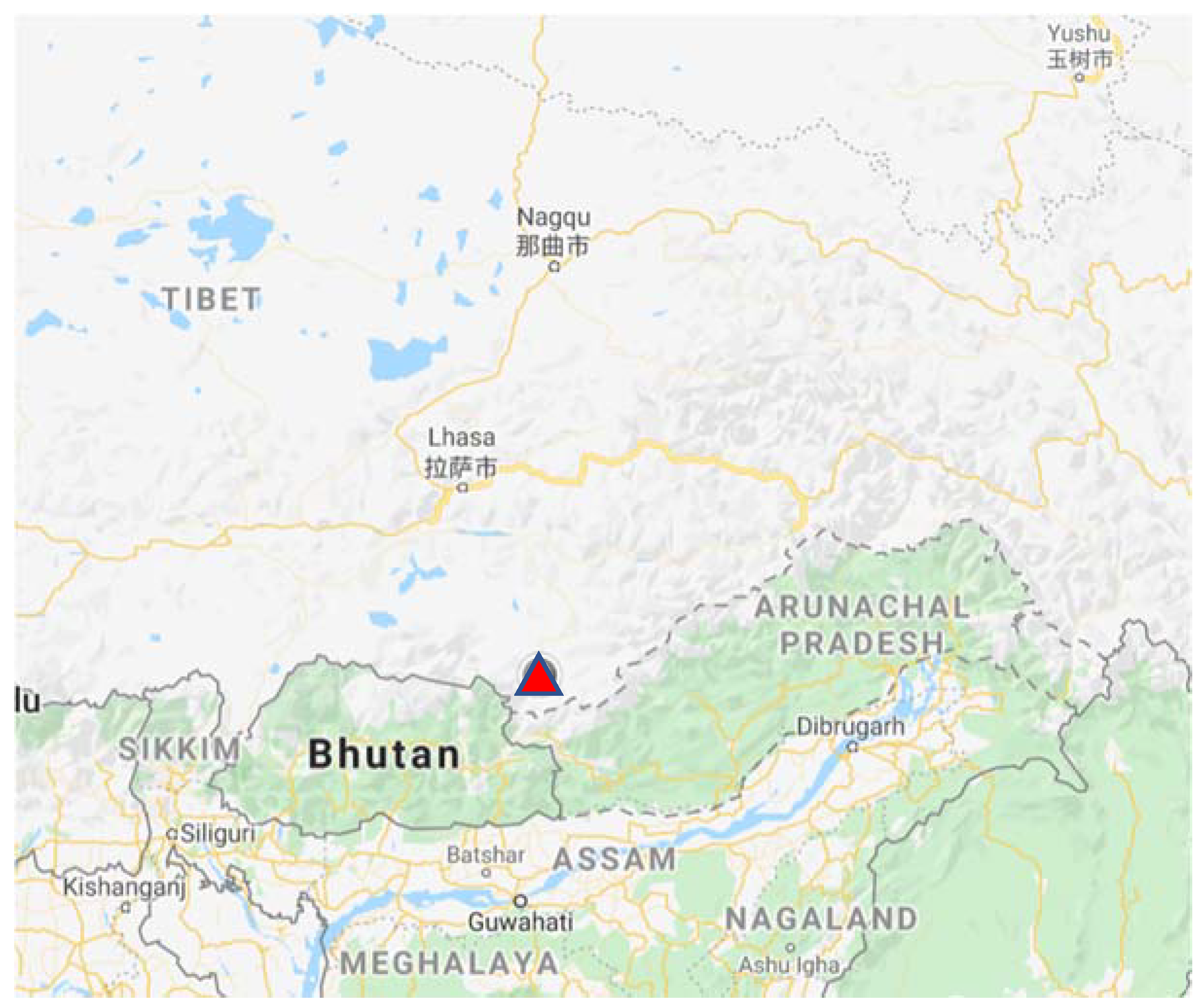
Cuona is a county located at the southern part of Tibet and the southeastern corner of the Himalaya Mountains. It is right on the boundary of two tectonic plates, European Plate and Indian Plate (Figure 1). The tectonic activities are very popular and there are a lot of dry hot rocks close to the surface. Because of this terrestrial property, the melted ice on the mountain at the western side of Cuona and the rain drops flow into the cracks on the ground surface and dip into the subsurface because of the gravity effect. It is then heated by the dry hot rock in subsurface area and stored in the water reservoirs underground. The hot springs are all over the small town, with the hottest ones with temperature over 100 °C [8,9].

On one side, Cuona has a higher elevation on the north side and has a relative height difference of about 7000 m, with the highest point of 7060 m and the lowest point of 18 m. Because of this high elevation and the influence of the Everest Mountain, Cuona has very long winters and short summers so that the supply of heat resource has always been a necessity for living. On the other side, the geothermal resource is prosperous in Cuona but because of the complicated geophysical conditions including faults and other pre-existing fractures, the exploration and production have always been challenging.

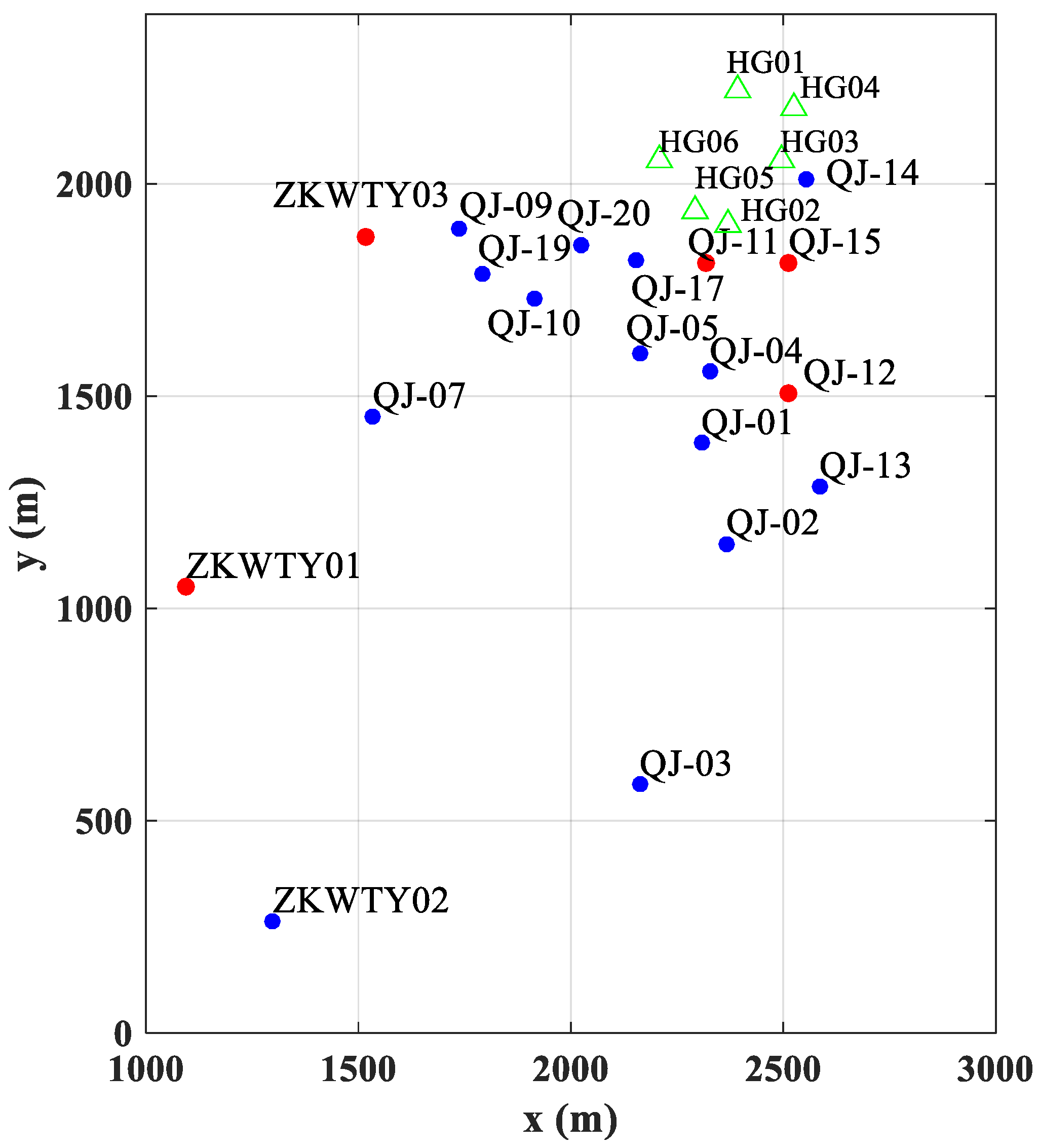
There have been many exploration and production operations, which accomplished their missions in the past so that Cuona has a running geothermal resource supply. The beginning of the geothermal exploration began in 1982, when one investigation team of Chinese Academy of Science performed an exploration job in this area and obtained some preliminary geophysical information. After that, there have been many other exploration activities in Cuona. For example, in 2012, the Geothermal Team of Tibet drilled two pilot wells and estimated the geothermal energy storage by measuring the water sample temperature, performing geophysical investigation and hydraulics measurements. This information provided the scientific foundation for geothermal exploration in Cuona for the first time. Two years after the geothermal project was approved, 15 geothermal wells were drilled and a geothermal project was built to provide heating for the houses in Cuona in September 2016. Right now, there are 18 wells producing warm to hot (17 °C to 64 °C) water to provide heating source for residents in Cuona. The locations of these wells are illustrated in Figure 2, where different abbreviation letters just represent different well groups. In Figure 2, blue dots represent wells with temperature less than 45 °C, red dots represent wells with temperature higher than 45°C and green hollow triangles are new drilled wells. It shows that the wells are mostly located in the northeastern corner of the city, which is also where one of the conjectured faults lies at. Two out of the three injection wells (QJ-01, QJ-04 and QJ-11) and two production wells (QJ-12 and QJ-15) involved in the tracer test are also located in this area.

While most of the previous operations have accomplished some production missions, there are many issues for existing geothermal production wells. Most of the previous projects were qualitative or at most roughly quantitative and they were not systematically designed. First, the production water temperature is not very high. The highest temperature is 64 °C (well QJ-15) and the lowest temperature is 17 °C (well QJ-03), with an average temperature of 40.5 °C. And out of more than 18 total production wells, there are only 9 wells with temperature higher than 45 °C. Second, the continuous production has caused the dropping of the groundwater level so that some of the spontaneous flowing wells are getting less water. Third, the connection relationships between 5 of the highest temperature wells are unclear, so that the injection plan is difficult to design. Finally, the remaining water after usage from the production wells is not used efficiently by directly pouring into the rivers. Some production information of these wells is listed in

Table 1. Basic information for 18 wells in Cuona.

Well#	Depth (m)	Temperature (°C)	Flow Rate m3/h	Well#	Depth (m)	Temperature (°C)	Flow Rate m3/h
ZKWTY01	1228.06	48	38.71	QJ-10	204.56	31	64.11
ZKWTY02	659.71	28	55.34	QJ-12	300.9	50	28.97
ZKWTY03	903.17	46	38.3	QJ-11	200.4	50	33.75
QJ-01	204.27	32	26.2	QJ-07	204.93	26	36.96
QJ-02	205.56	31	28.97	QJ-13	205.42	34	59.63
QJ-03	183.59	17	25.67	QJ-17	203.2	26	36.96
QJ-04	200.88	29	77.7	QJ-20	200.75	27	49.65
QJ-05	209.86	31	33.13	QJ-15	NA	64	50.44
QJ-09	204.08	37	33.13	QJ-19	204.43	41	58.75

, in which depth means the total vertical depth of each well and temperature is the highest water temperature.

With these existing issues and the urgent demand to have a sustainable geothermal production plan for Cuona, a good injection plan needs to be designed, from which the connection relationships between all the related wells can be investigated and quantified. To achieve that purpose, a tracer test was designed between 3 injector wells and 2 production wells. The tracer test data was collected and analyzed and corresponding streamline simulations and history matching procedure were performed to best match the tracer test result with different combinations of rock parameters and faults locations.

3. Tracer Test and Results

In order to make the geothermal project sustainable and the injection plan design economical, systematically designed field tests were performed in 2017. Based on the field test results, streamline simulations and history matching procedures are performed to find the possible subsurface geophysical environment so that the best injection plan could be designed.

3.1. Field Test

To prepare the tracer test and eventually design a better production plan for the geothermal wells in Cuona, some field work was performed during June 2017 to September 2017. In June 2017, rock and soil samples were drilled and analyzed. There are totally 77 samples, with 27 soil samples and 23 rock samples in drilling well 1 and 21 soil samples and 6 rock samples in drilling well 2. Drilling and sample testing showed that the geothermal brine is stored about 110–250 m deep under the surface, the porosity is around 5% and the components are mostly conglomerate, shales, rocks and soils, with soils constitute the most part.

3.2. Tracer Test

Tracer tests have been used widely all over the world to determine the connection relationships between multiple wells. For example, Pang et al. [10] described the tracer test performed in Xiongxian, Hebei province of China. The tracer test was done from January 2010 to July 2010, between 1 injector well and 5 production wells. In the end, there was no tracer detected from the production wells, so the production plan was abandoned, which saved a lot of money and time for the city.

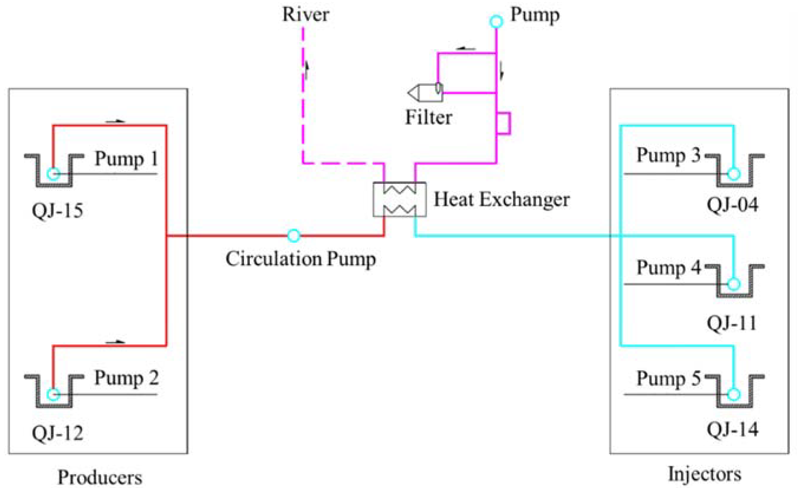
In September 2017, the tracer test in Cuona was performed by injecting water with three different kinds of tracers from QJ-04, QJ-11 and QJ-14 and the observation wells are QJ-12 and QJ-15. In our study, three different tracers applied here are 1,6-naphthalene disulfonate, 2,7-naphthalene sulfonate and 1,5-naphthalene disulfonate, injected for three wells QJ-04, QJ-11 and QJ-14 respectively. Our design of the tracer test is illustrated in Figure 3.

It is shown in Figure 3 that, after being filtered, the river water with environmental temperature was injected into the heat exchanger to cool down the hot water pumped from production wells QJ-12 and QJ-15 (left part of Figure 3, where red color means water with higher temperature), then the cooled water from production wells are injected to wells QJ-04, QJ-11 and QJ-14 to through pump 3, 4 and 5 respectively (right part of Figure 3, where blue color means water with lower temperature). After the water runs through the underground hot dry rock, the water absorbed heat and get a higher temperature and sequentially pumped up from pump 1 and 2 from QJ-12 and QJ-15 to the heat exchanger, for the purpose of heating and tracer test.

3.3. Results

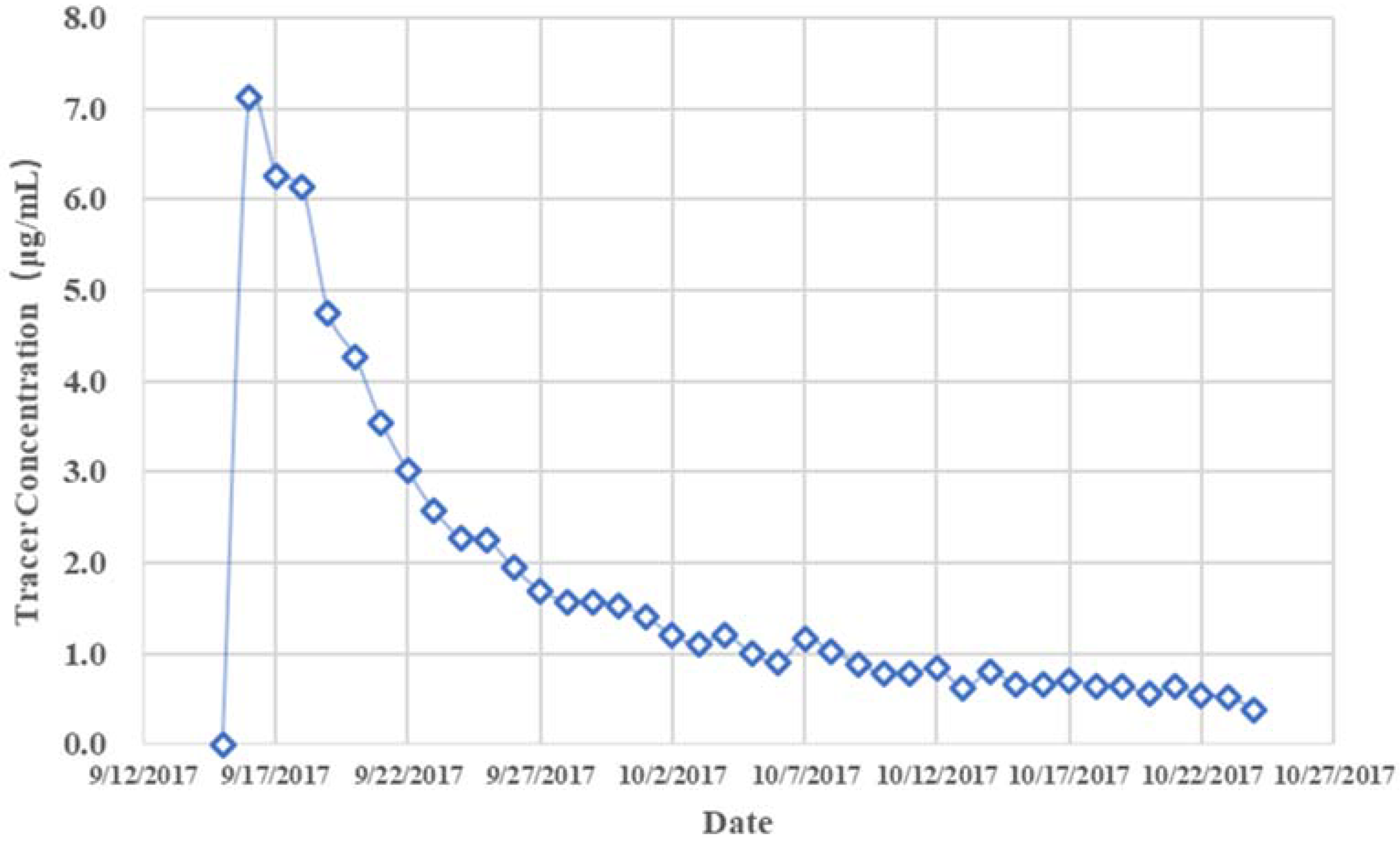
Before testing, standard solutions of 3 tracers have been tested and the testing procedure was validated. The error is within 0.01 μg/mL. Since injection began on 14 September 2017, water samples had been taken and regularly examined every day from two production wells, QJ-15 and QJ-12. In the end, only one tracer, 1,5-naphthalene disulfonate, was detected from QJ-15 well, which means the water injected from QJ-14 could flow to well QJ-15. The exact tracer concentration measurement is illustrated in Figure 4.

Figure 4 shows that the tracer was detected after 2 days of injection operation, with a concentration of 7.1 μg/mL, while the initial concentration of the tracer is 42.8 μg/mL. The concentration became smaller and smaller till 25 October when it became almost untraceable.

4. Streamline Simulation

In order to analyze the connection relations between the geothermal wells in Cuona, the analytical streamline simulation technique based on Complex Analysis was applied to history match the tracer results obtained in previous section. Sensitivity analysis was also performed so that the most possible geophysical properties can be proposed.

4.1. Application Background

As one of the most direct visualization method of fluid dynamics, the basic theory of streamlines and streamtubes in fluid transport problems was developed in Reference [11]. Since then many researchers have applied streamline methods to model fluid dynamics in oil, gas or geothermal reservoirs, both analytically [6,12,13,14,15] and numerically [16,17,18,19]. For example, Lake et al. [16] applied the streamtube model to simulate a large-scale polymer flooding and used analytical methods to solve for the fluid saturations. Datta-Gupta and King [19] suggested to replace streamtubes with streamlines thus solve the transport equation along the streamlines numerically. Zuo and Weijermars [20] illustrated the effect of the permeability and porosity of reservoirs on fluid trajectories and running time using theoretical derivations and numerical streamline simulations. Zhang et al. [21] and Zuo et al. [22] constructed the flux conservation techniques to compute the streamline across non-conforming grids such as grids with faults, local grid refinements and local grid coarsenings. Streamline methods have a variety of applications including computing injection and drainage volumes, tracer trajectories, reservoir sweep efficiencies and for history matching of reservoir models.

In this study, due to the limited data obtained by previous geophysical explorations, a sophisticated geothermal reservoir cannot be built, which leaves the opportunity to use simpler analytical methods and somehow facilitates our computation of flow trajectories and running time. That is because despite disadvantages of simplifying actual fluid mechanics, a key advantage of the analytical approach is that the explicit form representation of the complex potential allows the velocity field to be computed with high accuracy throughout the fluid domain, allowing fluid interfaces to be tracked sharply.

4.2. Streamline with Complex Analysis Method

In previous work done by the authors, the Complex Analysis Method has been used to simulate the velocity field in unbounded domain with impermeable fault [15] and in bounded domains [6]. For the completeness of this study, some related derivations and formulas are still summarized here. More details could be found in Reference [6] and other related publications [15,23,24].

In the Complex Analysis Method, it is assumed that all constituents of the reservoir can be modelled as a single phase incompressible fluid (which is good enough for geothermal modelling since we only deal with the single phase of water), except at a finite number of isolated sinks/sources, we arrive at Laplace’s equation for the dimensionless pressure P [11],

$${\nabla }^{2}P=0,$$

(1)

where ${\nabla }^2$ is the Laplace operator defined as ${\nabla }^2=\frac{{\partial }^2}{\partial x^2}+\frac{{\partial }^2}{\partial y^2}+\frac{{\partial }^2}{\partial z^2}$.

Denoting the complex coordinate $z=x+iy$, we can then write the complex potential governing the flow as

$$w\left(z\right)=P\left(z\right)+i\psi \left(z\right),$$

(2)

where $\psi \left(z\right)$ is the streamfunction (and note that the fluid pressure $P\left(z\right)=Re\left(w\left(z\right)\right)$. The velocity field is retrieved via

$$\frac{dw}{dz}\left(z\right)=u-iv.$$

(3)

In a domain with no impenetrable boundaries present, the complex potential at the point z owing to a collection of N isolated sink/source singularities can be written as

$$w\left(z\right)={{\displaystyle \sum }}_{j=1}^N\frac{m_j}{2\pi }\log \left(z-z_{a_j}\right),$$

(4)

where $z_{a_j}\left(j=1, \dots , N\right)$ are the locations of the singularities and m_j are their respective strengths (and are therefore real numbers). Now, consider a domain D_z consisting of M + 1 impenetrable boundaries on which the fluid velocity must satisfy

$$\mathit{u}·\mathit{n}=0,$$

(5)

where n denotes the normal direction to the boundary curve.

In most cases, the geothermal reservoir is usually considered to be bounded. Applying conformal mapping techniques, Equation (4) can be generalized to domains containing impenetrable boundaries. Our reference domain in which the complex potential is constructed will always be the interior of the unit ζ-disk with M excised smaller disks (one for each additional boundary present). Therefore, given a conformal mapping z = z(ζ) (with inverse ζ = ζ(z) from the reference D_ζ domain to the physical $D_z$ domain we have

$$W\left(\zeta \right)=w\left(z\left(\zeta \right)\right).$$

(6)

Note that, in geothermal projects, it is reasonable to assume that there is a set of ‘balanced’ sinks and sources with ${{\displaystyle \sum }}_{j=1}^N{m}_j=0$ corresponding to the assumption that all the water injected from the injector will be pumped and produced from the production well. And our domain is usually ‘simply connected,’ corresponding the case when $M=0$, the complex potential owing to a collection of point singularities located within the unit $\zeta$-disk can be written as,

$$W\left(\zeta \right)={{\displaystyle \sum }}_{j=1}^N\frac{m_j}{2\pi }\log \left[\left(\zeta -a_j\right)\left(\zeta -{\overline{a_j}}^{-1}\right)\right].$$

(7)

Thus, the fluid velocity in the physical domain is retrieved via the chain rule

$$u-iv=\frac{dW\left(\zeta \right)}{d\zeta }\frac{d\zeta }{dz}=\frac{dW\left(\zeta \right)}{d\zeta }\frac{1}{z_{\zeta }},$$

(8)

where subscripts denote the derivative with respect to the subscript. Complex potentials of this form and their resulting velocity fields can be computed efficiently using the open source and freely available potential theory toolkit for Matlab. Details regarding the numerical methods used in this toolkit are given in Reference [25].

Most geothermal reservoirs have impermeable faults [26]. When there is an impermeable fault in the area at location ($z_f$) in the reservoir, with arbitrary angle $\alpha$ and length $2L$, the velocity can be calculated as below [5,26],

$$\frac{dw}{dz}\left(z\right)={\displaystyle {\displaystyle \sum }_{j=1}^N}{m}_j\frac{\cos \left(r_j\right)-i\sin \left(r_j\right)\frac{1}{\sqrt{1-\frac{e^{2i\alpha }{L}^2}{{\left(z-z_f\right)}^2}}}}{\left(\cos \left(r_j\right)-i\sin \left(r_j\right)\frac{1}{\sqrt{1-\frac{e^{2i\alpha }{L}^2}{{\left(z-z_f\right)}^2}}}\right)\left(z-z_f\right)-\left(\cos \left(r_j\right)-i\sin \left(r_j\right)\frac{1}{\sqrt{1-\frac{e^{2i\alpha }{L}^2}{{\left(z_j-z_f\right)}^2}}}\right)\left(z_j-z_f\right)},$$

(9)

where ${\gamma }_j=Argu\left(k\left(h\left(z_j\right)\right)\right)$ and the mapping $h\left(z\right)$ and $k\left(z\right)$ are conforming mapping defined as the following,

$$h\left(z\right)=z+\sqrt{z^2-L^2}, k\left(z\right)=e^{-ia}·z$$

(10)

4.3. Streamline Simulation Results

In this work, the well strength $m_k$ can be converted by the actual well flux rates (Q_k) and porosity $\varphi$ using the following formula [20],

$$m_k=\frac{Q_k}{2\pi \varphi }.$$

(11)

Then the formulas provided in Section 4.2, specifically Equations (7) and (9) can be applied for the case of bounded domain with no fault and unbounded domain with fault, respectively. In the tracer test, the flow rates of three injection wells are constant of 20 m³/h and the flow rates of 2 production wells are constant of 30 m³/h, so that the equations listed above can be applied directly.

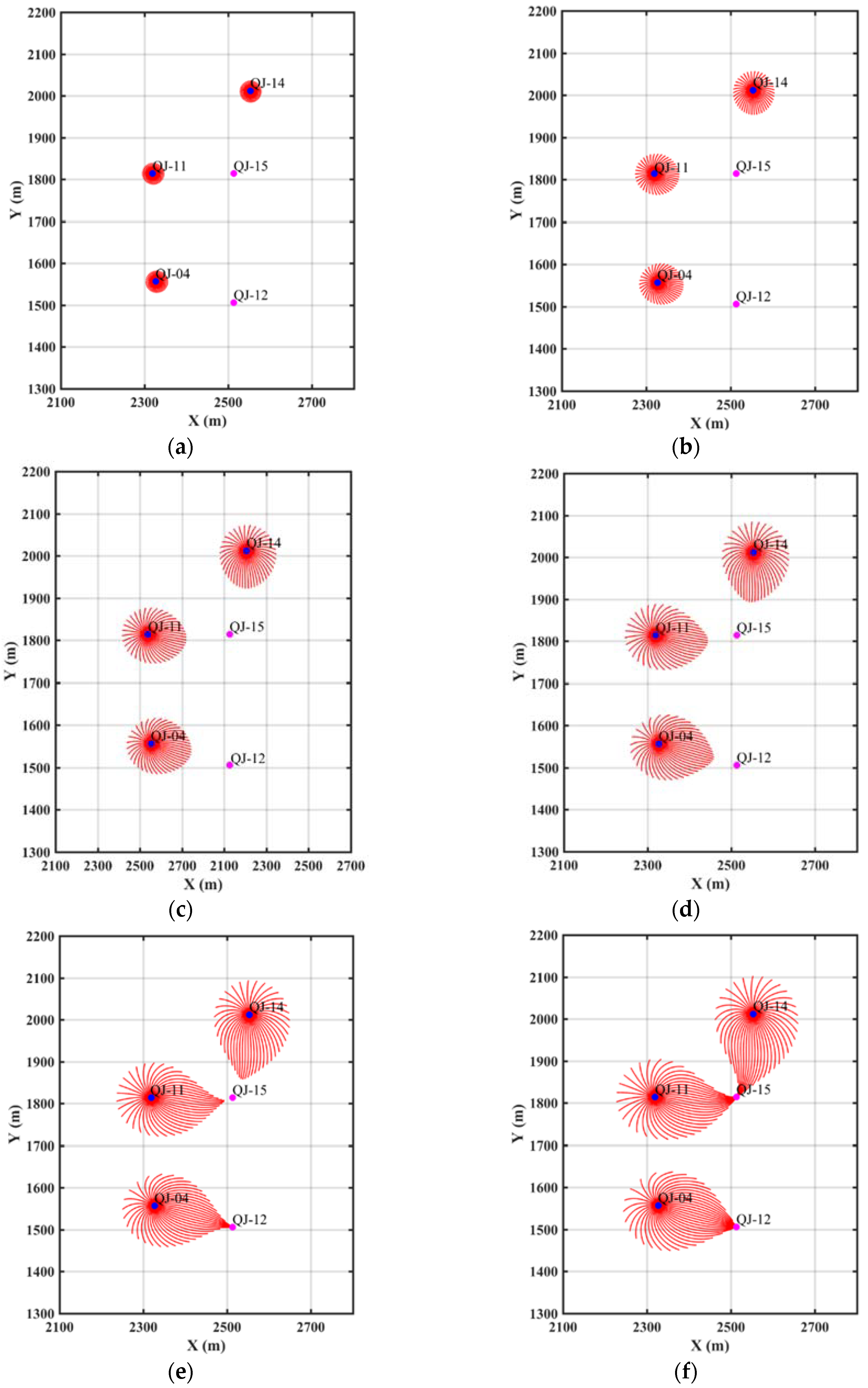
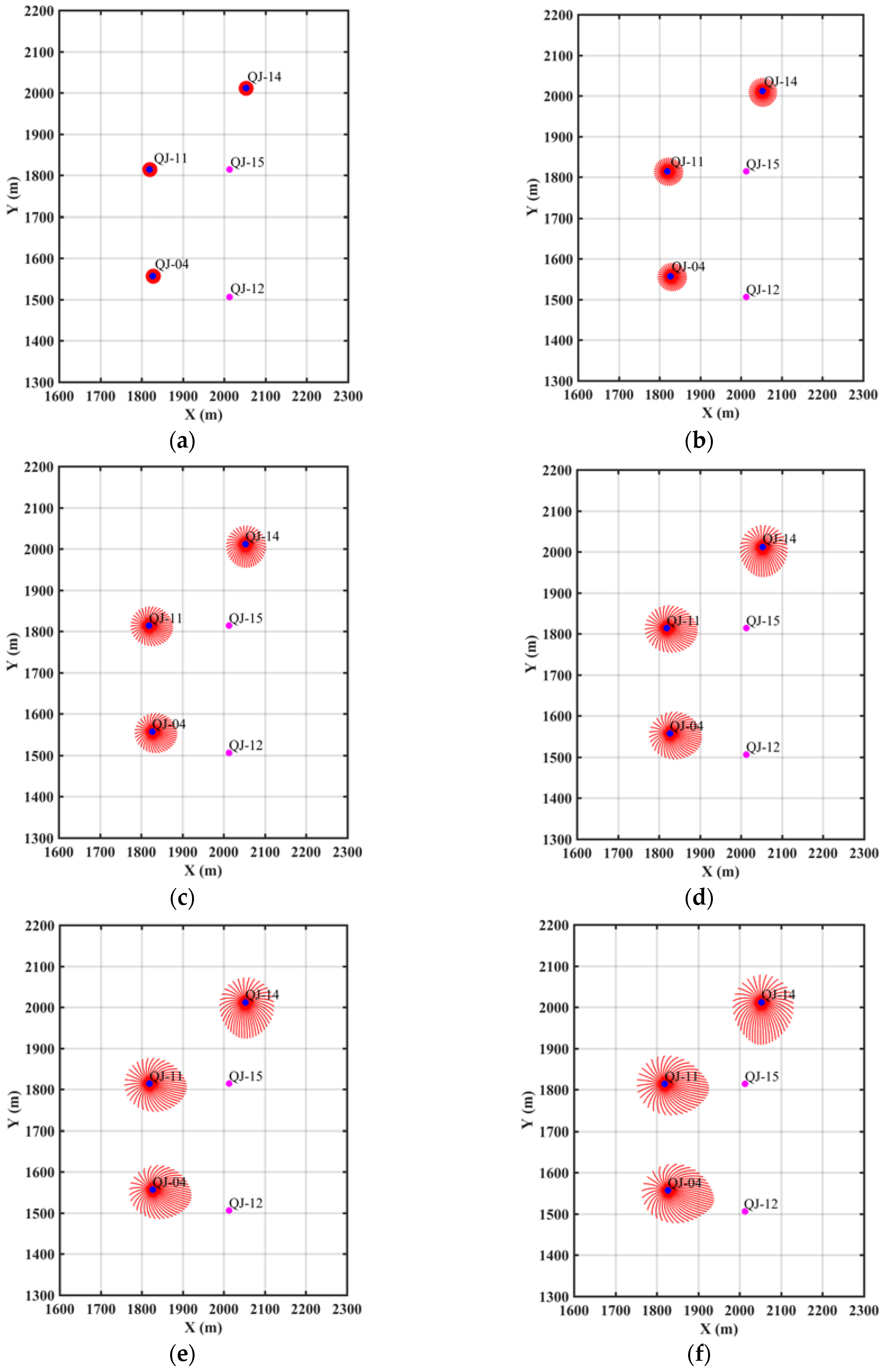
Assume other parameters are fixed, after adjusting the porosity and matching with the tracer arrival time shown in Figure 3, it is determined that the streamline results of porosity $\varphi =0.05$ is the best match, in which case the water injected from QJ-14 took 2 days to arrive at QJ-15. The streamline simulation results are shown in Figure 5.

To show the impact of porosity as one of the main model parameters, the corresponding results of porosity $\varphi =0.1$ are illustrated in Figure 6, which shows that the injection water of QJ-14 has not arrived at QJ-15 yet in 2 days. In fact, since the porosity is doubled, it can be predicted that in this case the water will need 4 days to arrive at QJ-15.

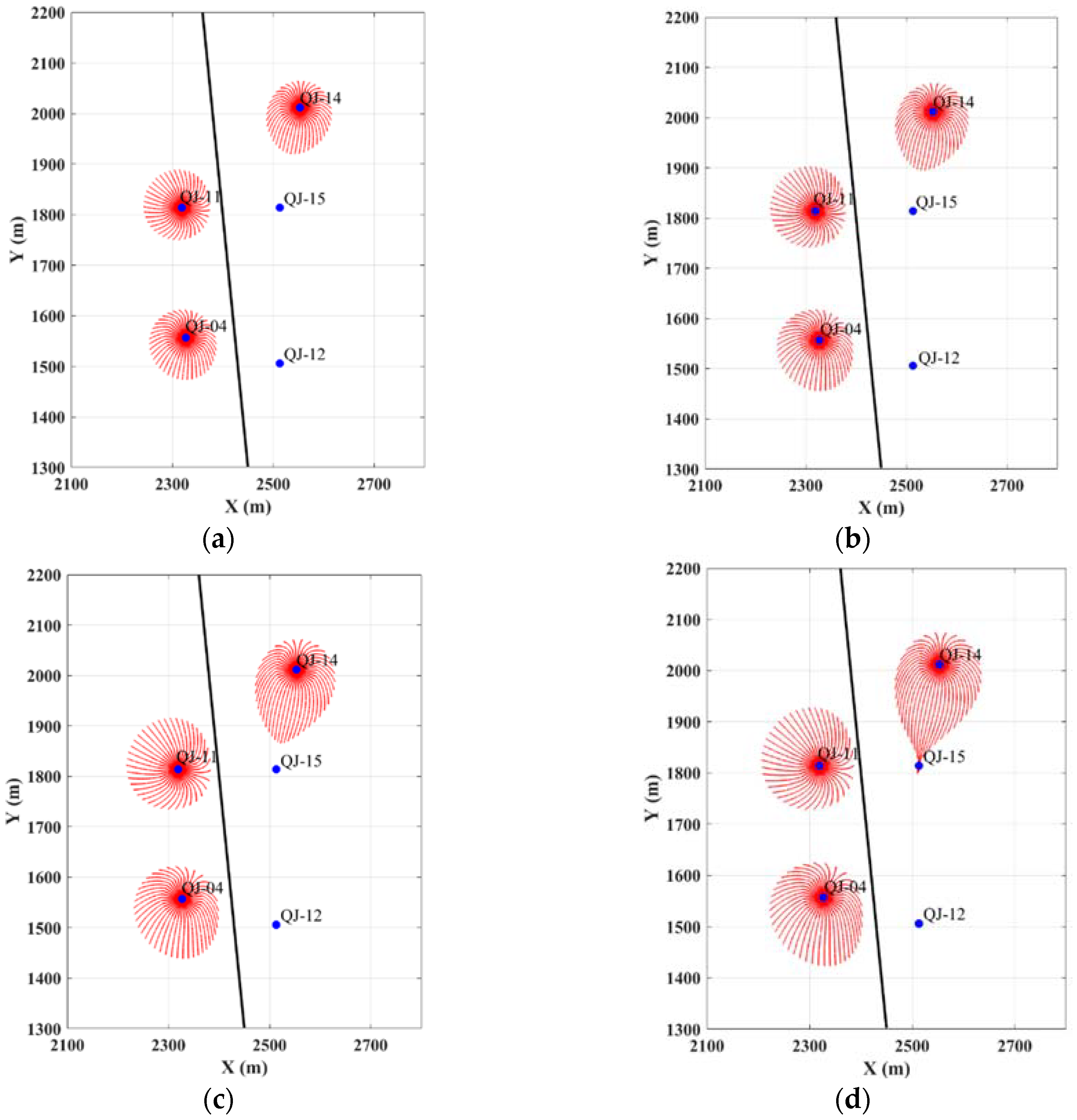
Since the geothermal reservoir model used here is the simplest one, without consideration of fault or fractures, which are very common in geothermal reservoirs, the streamline simulation results are not matching the tracer test results very well. For example, Figure 4 shows that there should also exist connections between QJ-11 and QJ-15 but in the tracer test, there was no tracer detected in QJ-15 from QJ-11. Similarly, no tracer was detected in QJ-12 from QJ-14. This is a good sign that there might be impermeable faults or fractures existing in this area. Some exploration geophysics evidences of the existence of faults in this area have also been reported by other researchers. For example, one exploration team found that in the drilling process of QJ-14 and QJ-15, clear drilling liquid loss happened at the depth of 80 m and the drilling sample is soft and different from other depths [27], which are good signs of the existence of faults.

In order to verify the existence of impermeable fault, a new streamline simulation based on Equation (9) was designed with one fault of 95 degrees lies between QJ-04, QJ-11 and QJ-12, QJ-14 and QJ-15, as shown in Figure 6. Here the angle is defined as the angle measure between the fault and the x+ axis. After running the simulation, it shows that the injection water from QJ-14 takes about 2 days to arrive at QJ-15, while the injection water from injection wells QJ-04 and QJ-11 were blocked by the impermeable fault, which explains why there was no tracer detected in production wells from QJ-04 and QJ-11.

In the case of impermeable fault as shown in Figure 7, the breakthrough curves of tracer test can also be predicted by using the streamline simulation results. In fact, as shown in Figure 7, the tracer took two days to run from injection well QJ-14 to production well QJ-15, so the concentration of tracer in QJ-15 before day 2 is just 0. Set the time t = 0 (in day) at day 2, then the quantity of tracer will decrease as the water was produced from QJ-15 with a flow rate of 30 m³/h = 720 m³/day, which means the mass of tracer satisfies the following first order ordinary differential equation,

$$\frac{dM}{dt}=-720\frac{M}{V},$$

(12)

with initial conditions, $M\left(0\right)=C_{0}V$, where $C_0$ is the initial concentration (7.1 μg/mL = 7.1 g/m³ in this study), $M$ is the total mass of the tracer and $V$ is the total water volume of the production well QJ-15, which is estimated to be 7200 m³ every day by using the multiplication of static water depth and well intersection area. Combing all the given values, the equation could be derived as

$$\frac{dM}{dt}=-\frac{M}{10},$$

(13)

with initial condition $M\left(0\right)=213$, in g. Solving Equation (13) by integrating both sides from time 0 to t and combining the initial conditions, we can get the solution as follows,

$$M\left(t\right)=213e^{-\frac{t}{10}}$$

(14)

so that the concentration of tracer is

$$C\left(t\right)=7.1e^{-\frac{t}{10}}.$$

(15)

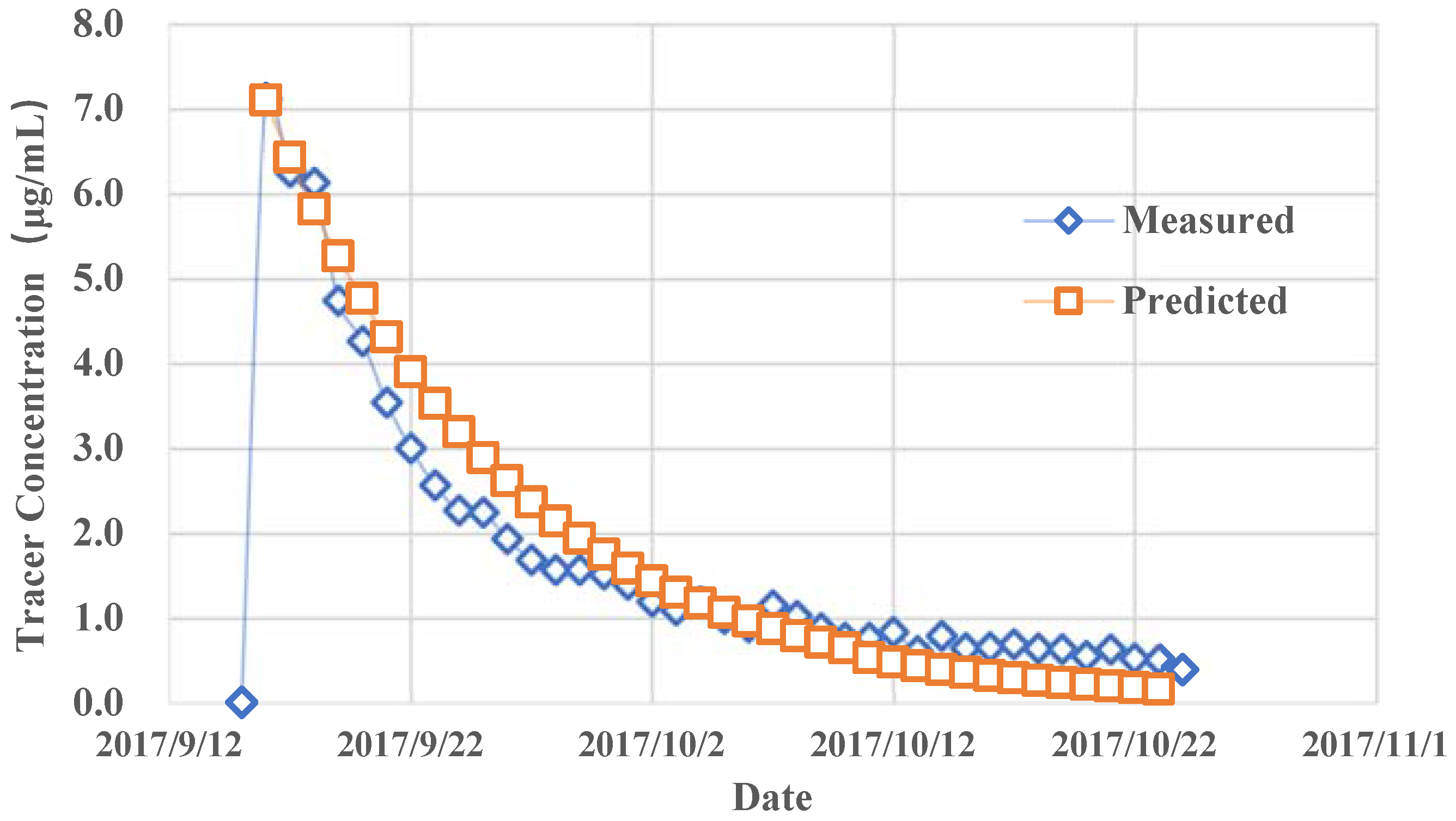
Using Equation (15), the predicted concentration of tracer with respect to time can be plotted together with the actual measurement of the tracer, in Figure 8. It shows that our streamline simulation combined with differential equation model could provide a reasonable match with measured data, although there are still mismatches due to the estimate errors of the well volume and other parameters.

5. Discussion

The geothermal energy has become an important contribution to the world energy supply, especially for areas where other energy resources such as fuel or electricity are difficult to harvest, such as Tibet. Due to high altitude, there is a great need for heating resources in Tibet for the whole year. Due to the challenges caused by complicated geophysical conditions, the geothermal resources in Tibet have not been well explored and produced and there are only limited amounts of geothermal projects managed by outdated techniques.

In this study, the well-established tracer test and streamline simulation were performed for the geothermal projects in Cuona, a county in southwestern Tibet, in order to design a better water injection plan so that the hot dry rocks could be more efficiently and environmentally friendly utilized.

Because this is the first time that the tracer test is implemented in Cuona, the test was not perfectly planned. Three tracers were injected from three different injection wells (QJ-04, QJ-11 and QJ-14) and water samples were taken from two observation wells (QJ-12 and QJ-15). It turned out that there was only one tracer detected from one inspection well QJ-15 and that tracer was injected from QJ-14. There are several possible explanations which are all reasonable for Cuona. First, since the tectonic movement is so frequent, the natural fractures and faults might exist all over the geothermal reservoir, while the current geophysical technique cannot detect and diagnose them accurately. In this case, the injection water will run through the natural fractures and permeable faults and arrive at different locations than the production well trajectories. Second, due to the same tectonic movement, there are impermeable faults generated in Cuona, which will act as a barrier between the injection wells and production wells, as is shown in Figure 7. But because of the lack of geophysical exploration data, it is impossible to determine which one is the main reason. With the development and application of advanced geophysical exploration techniques, more data will be available to make more accurate decisions.

On the other hand, if other factors, such as lower permeability zones, are ignored, it turns out that the existence of impermeable faults is the possible reason why there is no tracer going from injection wells QJ-04, QJ-11 to observation wells QJ-12, QJ-15 but the amounts and faults network is hard to be determined by the streamline simulation. The model proposed in our manuscript cannot be applied for heterogeneous reservoirs, which is one limit of this model. The tracer test result is the final combination effect of different factors, so that different faults and fracture locations and amounts could possibly lead to very similar tracer test results. In this case, the only possible solution would be developing accurate fracture and fault detection and diagnosis techniques.

To the best knowledge of the authors, this is the first time that a tracer test and streamline simulation has been applied to model the geothermal project in Tibet. Although there are some shortcomings of the current model due to the limitation of available data, this study will act as a good starting point for the geothermal exploration and production in Tibet, as more advanced and well-established techniques will be applied to help the production of geothermal resources.

6. Conclusions

To design a better geothermal production plan in Cuona, the tracer test was performed between 3 injector wells and 2 production wells in this study. The streamline simulation was used to assist the history matching and analysis of the reservoir properties. While the work is still on-going and the geothermal reservoir model is only 2 dimensional, there are already some interesting conclusions to draw.

• There exists a good connection between QJ-14 and QJ-15, because the tracer from QJ-14 was detected from QJ-15 in only 2 days. But the connections between other well pairs are poor, since after 45 days there were still no tracer detected between them.
• Ignoring the impact of other factors such as permeability and fracture distribution, streamline simulation shows that the porosity of the geothermal reservoir in Cuona is very close to 5%, since the water flow took 2 days to run from QJ-14 to QJ-15.
• One or more impermeable faults might exist in the geothermal reservoir, with an angle about 95°. These faults act like a barrier to prevent the water flow from QJ-04 and QJ-11 to the production wells.
• In complicated geothermal zones, the tracer test and streamline simulation could be applied to design the best injection plan and production plan by determining the connection relationships between multiple wells.