1. Introduction
Freestream turbulence is a feature to be found very commonly in flows of many kinds. It occurs in ducted flows as well as in unbounded flows and represents disturbances situated in the upstream history of the flow. It might, for example, result from the wake turbulence of objects, thermal bubbles or free shear layers. The freestream turbulence can have a significant effect on the flow along surfaces, where it affects boundary flow phenomena like transition and separation. Depending on its length scale it, either changes the magnitude and direction of momentum locally or even in larger regions.
In computational fluid dynamics (CFD) simulations with fully or partially resolved turbulence, the freestream turbulence needs to be accounted for. However, generally it does not appear feasible to resolve its formation, which often occurs far upstream of the focus region. Instead synthetic turbulence is applied. Several methods have been proposed using different mechanisms for the generation of synthetic turbulent fluctuations based on filtered random fields [
1,
2], vortex spot distributions [
3], reconstruction of measured spectra [
4,
5,
6] or reconstruction using proper orthogonal decomposition (POD) of measured time series [
7]. Often they are introduced into the computational domain as a boundary condition.
However, in applications from the field of external aerodynamics it is common to use boundaries of farfield type for the outer edge of the computational domain in order to investigate the flow around a free flying object with the boundary being as unaffected as possible by the object in focus. Most of the computational domain is not of interest in the investigation and therefore usually is resolved very coarsely, which also filters out disturbances approaching the boundary. Introducing synthetic turbulence in a farfield boundary condition would then require a grid resolution fine enough to fully resolve the turbulent structures in order to transport them convectively up to the focus region. Furthermore a long time span would have to be simulated until the turbulence arrives at the investigated object. Besides the high computational effort, the decay of the turbulence during this time would also have to be considered in prescribing the boundary condition.
Since this appears unfeasible, different approaches have been proposed to introduce turbulence closer to the focus region. It is, for example, possible to introduce turbulence by superposition from an overlapping mesh as proposed in [
8]. This requires the solver software being capable of handling mesh overlays. Alternatively, volumetric force fields can be applied to manipulate the flow field. Numerical simulations of volume forced turbulence are most often formulated in Fourier space, where forcing [
9,
10] or stochastic forcing [
11] is typically applied to low wave number modes. A comprehensive overview for such spectral forcing schemes can be found in Rosales and Meneveau [
12]. It is generally accepted that forcing the Navier–Stokes equation at low wave number does not influence the small-scale statistics of the flow, provided that there is a wide separation between the largest and smallest scales [
13]. Similarly, the spectral nudging method developed by Waldron et al. [
14] imposes time-variable large-scale flow states on a local model and is often used for regional climate modeling [
15].
However, many engineering problems do not admit periodic boundary conditions and the solution cannot be expanded in a Fourier series. They are often simulated using numerical codes formulated in physical space such as finite volume methods and consequently spectral forcing is difficult to implement [
12]. In the linear physical space forcing proposed by Lundgren [
13], the force is proportional to the velocity fluctuation. While this is an attractive approach, which has been well characterized in [
12], it has been also demonstrated that the length scale converges to an average scale near 35% of the domain size (based on the estimate
) independently of the initial conditions and the situation becomes even worse on non-cubic domains [
16]. In order to control the length scales it has been suggested in Klein et al. [
16] to make the forcing proportional to a high pass filtered velocity fluctuation. However, implementation of a high pass filter on an arbitrary unstructured grid is not straightforward. Recently, Schmidt and Breuer [
17] have proposed a method based on applying a local volume force to superimpose synthetic turbulence at arbitrary locations of the computational domain, which can relatively easy be integrated into a Navier–Stokes solver by adding a source term.
The present work introduces an approach based on the latter method. Treatment of the source term in the pressure correction algorithm is addressed, as well as monitoring and scaling the resulting turbulence by supplementing it with a controller mechanism. The approach then is calibrated using a simple channel setup with free slip walls, validated using a farfield configuration and further assessed with respect to performance with the flow around a cylinder with an alternating vortex street pattern. Finally, results of the flow around a NACA0012 airfoil at high angle of attack with and without freestream turbulence will be presented and discussed. Applying the method in all these cases demonstrates the generality of the method.
2. Numerical Method
For the flow simulation an incompressible flow solver from OpenFOAM has been used. It solves the Navier–Stokes equations in an incompressible formulation. Pressure and velocity are coupled using a dual time stepping pressure correction method combining PISO time steps with outer iterations of the SIMPLE algorithm.
According to Schmidt and Breuer [
17] a locally acting force is introduced to the momentum equation, which then, in the commonly used incompressible form of OpenFOAM with the pressure normalized by the constant density, becomes
The force needs to be set appropriately in order to achieve the desired velocity fluctuations. Typically, the force is only acting in a certain zone upstream of the focus region. The volume force represents the force which is necessary to accelerate the fluid to the desired fluctuation velocity. It depends primarily on the transition time T a fluid element spends traveling across the influence region and the fluctuation velocity vector.
To stabilize the numerical solution, the force should not introduce sudden jumps into the momentum equation. Therefore a Gaussian bell-shaped function
G is introduced to soften the force field towards its boundaries. To preserve the total force effect,
G is normalized by its mean value
. Assuming that the undisturbed flow primarily is pointing in the
x-direction, the transition time can be calculated from the width of the forcing zone
and the
x-wise bulk velocity
. The force term superimposing a fluctuation velocity
then is expressed by
At very low levels of turbulence intensity the bell function primarily is acting to smooth steps in the stream-wise direction. For stronger turbulence it is necessary to also smooth the force field towards the sides of the forcing region unless they reach the boundary of the computational domain. Thus, depending on the specific setup, a two- or three-dimensional function is applied.
The additional force term in the momentum equation needs to be taken into account in the pressure correction. An additional term arises in the pressure equation representing the divergence of the force field. The semi discretized form according to Jasak [
18] then becomes
where
denotes the matrix coefficient for the central cell and
represents the neighbor cells and the temporal derivative. It needs to be mentioned that, if the forcing term is implemented correctly in OpenFOAM,
will also incorporate it as a source term. However, in an intermediate step this has been prevented here for the sake of demonstration.
For an ideal transfer of the fluctuations into the fluid flow it would be necessary to move the force field along with the flow across the forcing zone. In order to facilitate the implementation of the method and its computational overhead just one slice of the force field is taken at a time and spread across the forcing zone. That means, that the local force changes, while a fluid element is passing. This changes the amount of force applied depending on the ratio of the length scale of each fluctuation to the forcing region length. The wider the forcing zone is selected the lower the fluctuation magnitude will become. On the other hand it is desirable to have a wider forcing zone for a smoother transition into and out of the force field.
The effect of forcing zone width on the resulting fluctuation field is illustrated in
Figure 1. In order to give a clearer view to the fluctuations, they are in this context applied to a passive scalar field. The scalar is transported only convectively with a constant bulk velocity. The upper image of
Figure 1 shows the original field of synthetic fluctuations. Below the resulting fields from calculations with different settings for the width of the forcing zone are shown. The length scale
of the fluctuations generally is produced well. Some structures, where two or more spots are very close to each other become blurred and the individual spots form one larger spot in the resulting field. This happens regardless of the forcing zone width.
The effect of the width is most obvious in the lower image where the width is four times the fluctuation length scale, which for practical use definitively is too big. The primary consequence is, that the resulting spots are much less intense, which results from the mechanism described above. This also appears for the other cases with different length scale ratios shown in
Figure 1. It is less obvious but still measurable and significant since it changes the resulting mean fluctuation intensity.
Another effect which modifies the introduced fluctuation velocity is, that the pressure correction algorithm reacts to a positive acceleration with a positive pressure gradient unless the acceleration field is free of divergence. Thus the accelerating force is partly balanced by a counteracting pressure gradient. This effect is relatively small in weak turbulence and only relevant for intense turbulence at larger scales. Finally, besides these effects, which arise from the numerical treatment, the viscous decay of turbulence also alters the turbulence intensity between its introduction until it reaches the focus zone.
To overcome all of these effects a control loop has been introduced. Applying a mechanism to control the generated turbulence has been proposed previously [
16,
19,
20] with proportional correction terms. In the present work a full PID controller has been applied. An amplification factor is applied in Equation (
2), which scales the force field globally. Downstream of the forcing region a control region needs to be placed, in which the resulting fluctuation intensity or the turbulent kinetic energy is measured. In order to reduce local variations of turbulence intensity as the fluctuations are passing by, the control region should be selected sufficiently wide. At each time step, the mean value of
is calculated inside.
The difference between the actual and desired fluctuation velocity, the error variable
, is determined. The calculated error is then processed in a common PID control function, which thereby determines the control variable.
Here, denotes the control output and K the gain coefficients for the individual controller terms.
The controller is implemented in a discrete formulation, where the integral is replaced by a sum of all measured error terms and the derivative is approximated by finite differences.
The controller output u is then added to the force amplification factor, which results in another integral effect. It has proven beneficial to limit the amplification to positive values since negative scaling is not appropriate.
For the performance of the controller it is essential to select an appropriate set of gain coefficients. They depend strongly on the individual setup, namely the delay times, which arise from the propagation of fluctuations from the formation within the forcing zone until they reach the measurement zone and further until they have completely passed and filled the measurement zone. The first part can be considered as dead time
since the scaling effect is not being measured, yet. In the present work it is defined as the time needed to come from the middle of the forcing zone to the beginning of the measurement zone at bulk velocity. The second part, the passage through the measurement zone at bulk velocity, can be considered as the rise time
of the measurement. From simulations of a two-dimensional slip-wall channel with synthetic fluctuations the following correlations have been developed inspired by the criteria according to Chien, Hrones and Reswick [
21]. The setup for calibrating the controller parameters has been selected two-dimensional, because not the development of actual turbulence but only the presence of fluctuations is of importance in this context. Thus a two-dimensional case decreases the computational effort significantly.
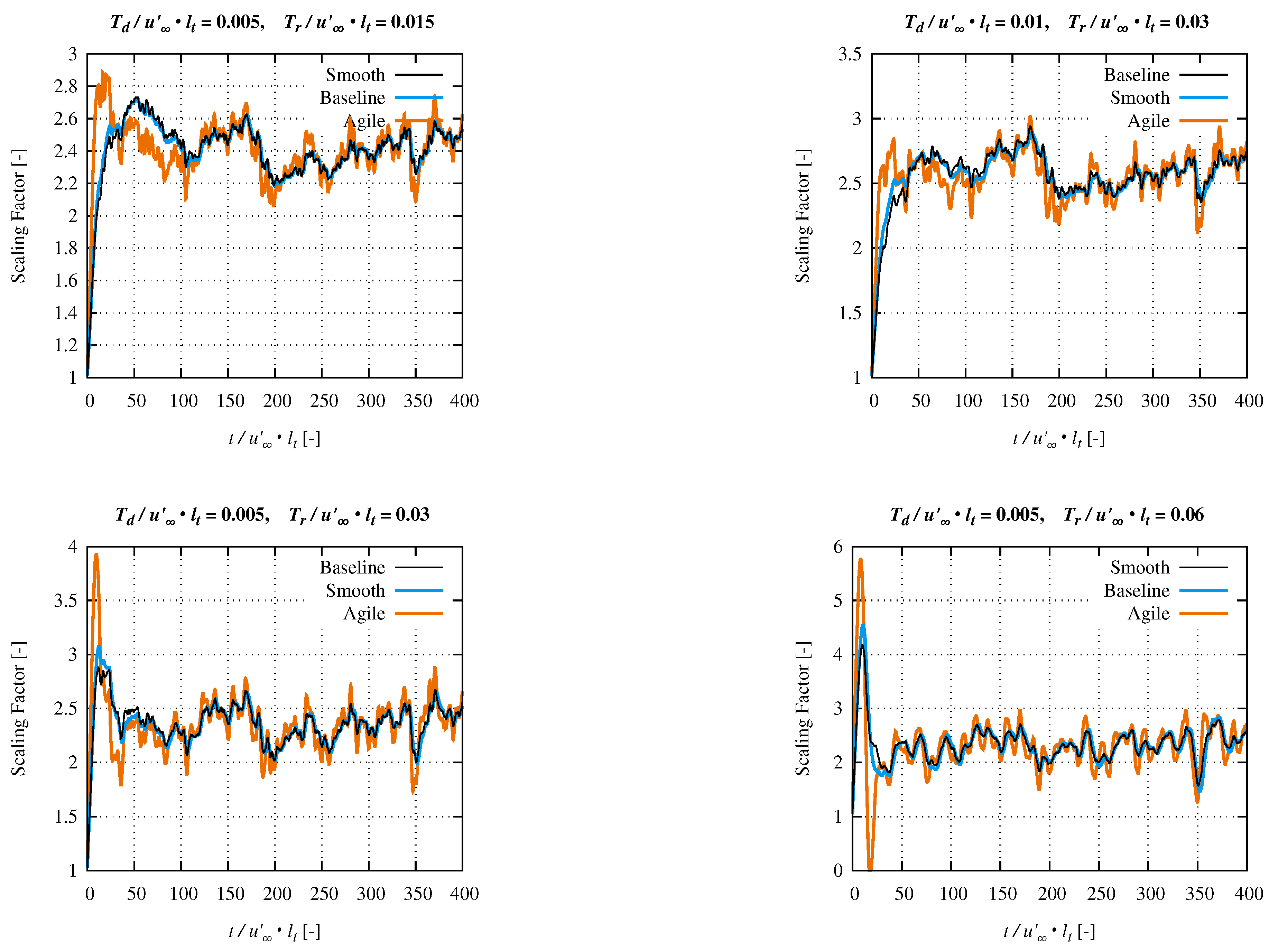
Three different tunings are presented in
Table 1. The baseline setting generally showed good results in keeping the measured error low as well as not allowing too much variation of the scaling factor. The smooth setting allows for slightly more measurement error variations and makes the controller reacting slower. This leads to a smoother behavior of the scaling factor. In the agile setting the controller allows quicker adaption of the scaling and reduces the measured error. It also tends to produce an overshoot in the initial phase. The evolution of the amplification factor for these three tunings is shown in
Figure 2 for a channel flow with 10% fluctuation intensity. The width of forcing and measurement zones is varied, which leads to different delay and rise times, respectively. Setting the width of the forcing zone to approximately the fluctuation length scale appears reasonable. With the measurement zone being two to three times as wide as the forcing zone the rise time can be kept low while still taking advantage of the smoothing effect by its size.
One might expect, that the coefficients should be dependent on the target fluctuation intensity. Taking such a dependency into account, indeed leads to a very quick response of the controller and the desired intensity level is reached soon. However, afterwards the scaling factor will show too strong variations. Instead it is advisable to estimate an initial setting for the scaling and delay the controller activation by , which will ease the initial adaptation.
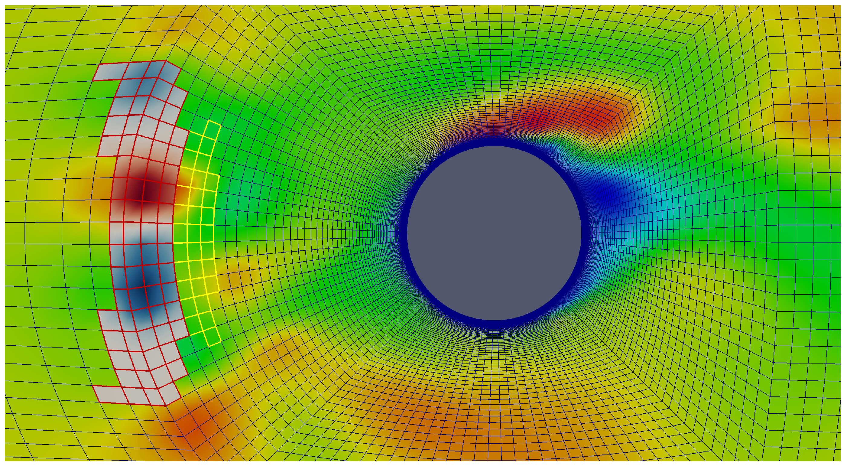
The schematic sketch for a practical application, an airfoil flow, is shown in
Figure 3. One slice of the synthetic fluctuation field is applied in the red forcing region. The result is measured in the yellow control region and fed back through the controller. The resulting turbulence field is indicated by blue iso-surfaces of Q criterion.
In all cases presented here the synthetic fluctuations have been generated using a method proposed by Kempf et al. [
2] based on diffusive filtering of a random field. Depending on the amount of diffusion applied, the length scale can be controlled. Finally, the field is normalized and transformed to fulfill the prescribed intensity or, if the specific applications requires this, even the full Reynolds stress tensor using the transformation by Lund [
22].
It is worth noting that the forcing method is completely independent of the generation method and it can be combined with synthetic or real turbulence from an arbitrary source. It is not necessary, that the fluctuation field is free of divergence. Unlike in a synthetic turbulence boundary condition as proposed by [
23] the volume force will not generate divergence of the velocity field beyond the limits of the pressure correction algorithm after the solution of a time step is converged.
3. Results and Discussion
3.1. Validation in Empty Domain with Farfield Boundary
The first step in the validation process is to verify that the fluctuations induced into the simulation domain agree with the prescribed statistical properties. To ensure that the turbulence does not interfere with geometry an empty farfield domain has been simulated. The setup is based on the flow around an obstacle like an airfoil. The entire domain extends 20 units of length in stream-wise and vertical direction with a farfield condition along the outer boundary. Its span-wise extension is 0.5 units with periodic boundaries. The unstructured hexahedra-based mesh features cells with hierarchical refinement towards the central region. Between the stages of refinement polyhedral cells are introduced to avoid hanging nodes. The fluctuations are introduced in the range of to immediately followed downstream by the controller measurement region up to . If an airfoil was present it could be expected within and and the refinement is kept further up to . In perpendicular direction the refined area extends between and . This is equivalent to the extension of the forcing region with the forcing being smoothed out towards top and bottom as described above.
The prescribed turbulence is set to a relatively low value of and an integral length scale of units of length. Even though the method would allow to specify individual components of the Reynolds stress tensor, in the present case only a homogeneous turbulence intensity has been prescribed using the diagonal tensor components. The Reynolds number based on one unit of length is 80,000.
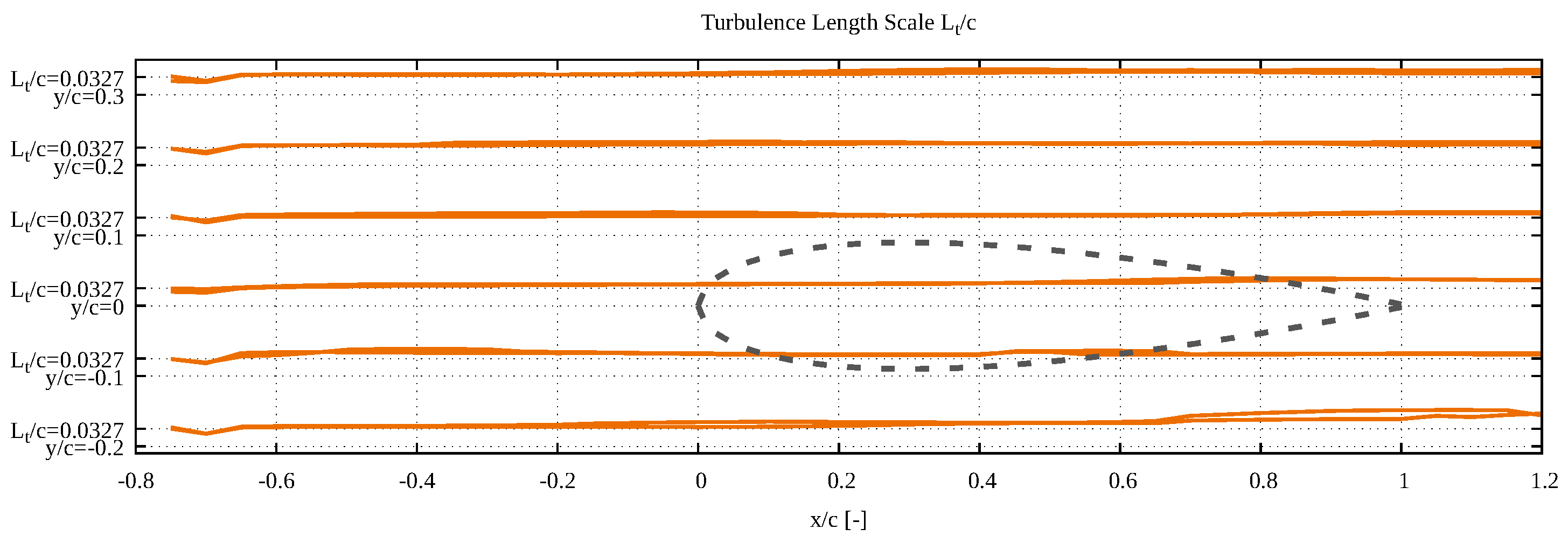
With this setup, after sufficient initial relaxation time, data have been collected for 10 convective time units, from which the achieved mean fluctuation intensity as well as the actual integral length scale, calculated from autocorrelation, have been determined. The development of both values is shown in
Figure 4 and
Figure 5, respectively, along lines ranging from the forcing zone through the fine mesh region in six vertical locations. Each of these is covered by two lines in periodic direction, which mostly coincide in the plots therefore showing only one line. An airfoil shape, which not has been present in the computations, is indicted in the figures by dashed lines to show a possible application setup.
It can be seen that after passing the forcing zone both quantities reach the prescribed values. In the topmost and lowermost lines the intensity stays slightly below the target value since the damping function towards the edges starts acting. During the downstream propagation, the fluctuation intensity shows a very slight decay as it can be expected. Accordingly, the value of the integral length scale rises slightly as the fluctuations decay. These results give confidence that the entire setup of forcing and controlling reliably produces the prescribed fluctuation properties and can be applied to more complex applications.
3.2. Performance Assessment
By introducing the controller mechanism the magnitude of the original input fluctuation field becomes irrelevant. Only the length scale and, if required, the cross correlations of the Reynolds stresses need to be prescribed correctly in advance. The magnitude of the fluctuations can then be amplified to an arbitrary value. Thus, series of simulations with variation of the turbulence intensity are possible with only a single set of synthetic fluctuations.
To demonstrate and validate this capability the two-dimensional flow around a cylinder with synthetic fluctuations in the approaching flow has been calculated with different settings for the turbulence intensity. Here, again, two-dimensionality has been chosen to reduce the computational effort. The demonstrative purpose is to show the behavior of the controller and not that of the turbulence field.
The setup is shown in
Figure 6, the forcing zone is located one diameter upstream of the cylinder and 1.5 times the diameter downstream of the inlet boundary. It extends up to five cells in stream-wise direction, which appears to be sufficient for stable operation. The measuring region of the controller is located immediately downstream of the forcing. For the controller it would be favorable to increase the width of the measurement zone. However, since the cylinder is affecting the flow upstream it is not suitable to further increase the measurement zone in this case.
From one field of synthetic fluctuations four different simulations have been performed with different levels of
. They range from from almost undisturbed flow (
) to high turbulence (
). At a Reynolds-number of
, based on bulk flow velocity and diameter, the cylinder wake flow forms a characteristic von Karman vortex street, which is disturbed by the approaching fluctuations. An instantaneous view to the flow field is given by
Figure 7 for the highest setting of turbulence intensity after sufficient computed time to achieve a relaxed quasi-steady state. The smaller scale eddies become dissipated very quickly downstream of the cylinder because the mesh is getting coarser.
The controller reaches the prescribed turbulence level approximately within one to five characteristic time units (
) depending on the intensity level as illustrated in
Figure 8. In the case with lowest turbulence intensity the amplification factor drops close to zero (where it is bounded) remains zero after about twelve CTU, when the vortex street has fully developed. The reason is, that the vortex street induces very small variations of the velocity upstream of the cylinder. These are recorded by the controller and in this case they are sufficient to pretend the presence of enough synthetic fluctuations. To overcome this, the mechanism would have to be placed further upstream of the cylinder, where no upstream influence of the vortex street is measurable. Consequently, this case is almost identical with a case without freestream fluctuations.
In the case with highest turbulence intensity a drop of the scaling factor at twelve CTU appears in the plot. This is a combined effect of one particular event in the synthetic turbulence field and the integral error term vanishing at the end of a slight controller overshoot. Hence afterwards the scaling coefficient remains at a slightly lower value.
The effect of turbulence in the approaching flow is, that the vortex street forms sooner. The fluctuations help breaking up the shear layer and form instabilities.
Figure 9 shows the temporal evolution of the lift coefficient. In the case with the lowest turbulence the longest time is needed to achieve the final amplitude of the alternating vortex separation. In the second case the development of the vortex street happens slightly sooner and it then reaches its final amplitude after a shorter time. The appearance of the lift curve still is regular with only slight disturbances.
In the third case the separation starts almost immediately compared to the previous two cases. The influence of the fluctuations is clearly visible but also the characteristic of the alternating separation remains visible in the lift plot. In the case of highest turbulence intensity the alternating pattern almost vanishes while the force is dominated by the fluctuations. The coefficient reaches values far higher than those seen purely from the vortex street. The events indicated by the drop of the amplification factor around twelve CTU also are visible in the lift coefficient as the pattern changes in the same interval. As also visible from the velocity field in
Figure 7 the vortex street is still present but it is deformed by the fluctuations.
In order to determine the significance of modifying the pressure equation by introducing the force term the same set of cases has been calculated again with the original pressure equation and the forcing term only being present in the momentum equation. As long as the iterative procedure of the PIMPLE algorithm converges, this is supposed to reach the same converged state for each time step as in the previous setup but might need more corrective iteration steps for the pressure equation. The result of the comparison is presented in
Table 2.
For all four cases the computing time and the number of iterations performed to achieve the convergence of the pressure correction algorithm are compared. The data is taken from a calculation at quasi-steady state simulating a range of five CTU starting after the first twenty CTU. In the first case it needs to be reminded, that the controller mechanism has faded out the turbulent forcing for most of the time. This still produces overhead to handle the zero-forcing in the pressure equation and leads to an increase of computing time. However, the number of pressure correction iterations decreases during the short phases, at which the amplification becomes greater than zero. This results in a slight decrease of the total number of pressure correction iterations.
For the three cases with significant fluctuation level the result changes considerably. The number of pressure iterations decreases by more than ten percent and up to thirteen percent. The reduction of computing time is not as big as the decrease of pressure iterations but still significant. It ranges from six to almost eight percent. It appears to be independent of the fluctuation magnitude. However, the difference for each case certainly has a strong dependence on the solver settings and can vary for different applications.
3.3. Airfoil in Freestream Turbulence
As mentioned before the two-dimensional cases presented here have been selected in order to reduce computational effort for validation and demonstration. Actual turbulence needs to be studied in three-dimensional applications to resolve the three-dimensional aspect of turbulent motion correctly. Such turbulence-resolving computations require parallelization to achieve results within reasonable computing wall time. It should be noted, that in a parallel computation the controller requires intercommunication between the parallel processes, which are involved in measurement and forcing, to produce one uniform amplification factor.
The flow around a wing is known to be very sensitive to freestream turbulence. Particularly at low Reynolds numbers, when the flow tends to separate easily, freestream turbulence changes the separation process significantly. While large scale turbulent eddies in the order of the chord length change the angle of attack globally, smaller eddies affect the momentum in the boundary layer and thus have an impact on transition and on separation of the flow.
In the present case a NACA0012 wing has been investigated in freestream turbulence. The case is quasi two-dimensional with periodic conditions in span-wise direction. The computational domain size in periodic direction is 50% of the chord length. The outer boundary is of farfield type and located 20 times the chord length from the wing. The mesh is of structured C-type topology even though it is treated in an unstructured way by the flow solver. The total number of cells results in . Gradients of the boundary layer are resolved in wall-normal direction with a of the first cell layer well below unity. and are selected higher using values of 30 and 50, respectively. The mesh is designed to be used with a k--SST-DDES turbulence model, which resolves large eddies in the separated flow region and models the immediate wall boundary layer turbulence using the k--SST two-equation model.
At an angle of attack of 12 and a Reynolds number of 50,000 based on freestream velocity and chord length the flow is separated along almost all the upper side of the wing. Therefore a very unsteady behavior with vortex shedding in the shear layer above the separation zone can be observed.
Freestream turbulence is applied with 10% fluctuation intensity based on the freestream velocity. The length scale is 10% of the chord length. This has primarily an effect on the boundary layer and shear layer momentum balance. It affects the vortex shedding and enhances the turbulent breakup of shear layer vortices, which then can reach the wing surface. Local variation of the angle of attack plays only a minor role.
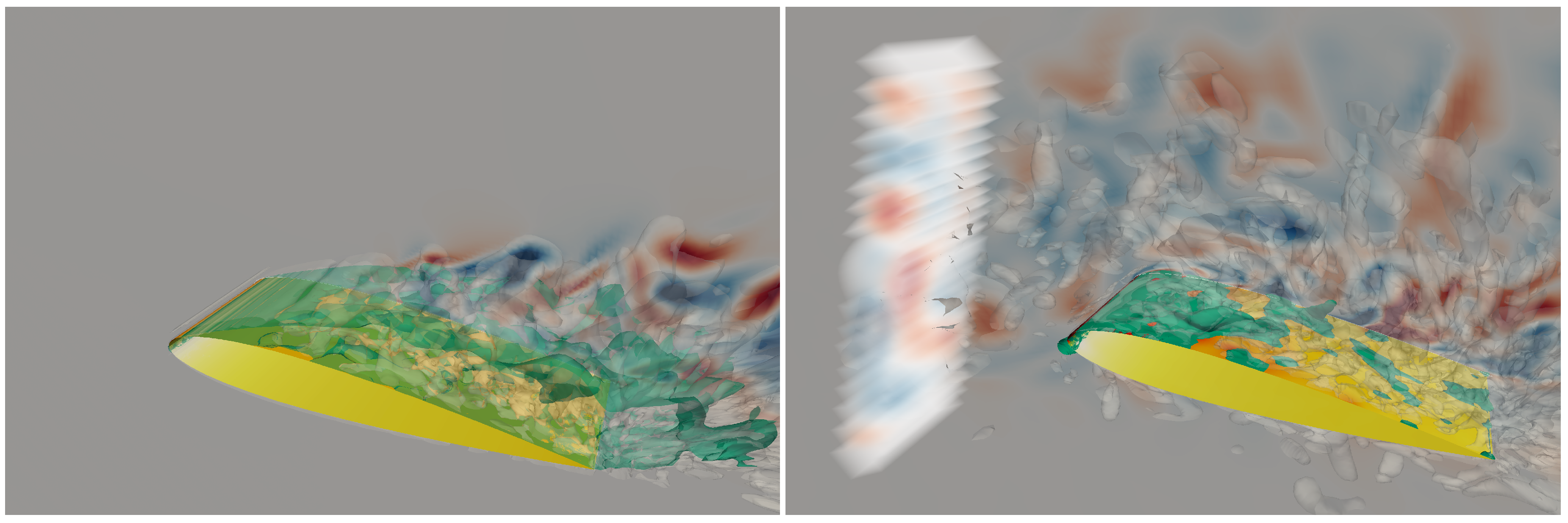
Figure 10 gives an instantaneous view to the flow in laminar and turbulent freestream conditions. The separated regions are marked by the green iso-surfaces of zero stream-wise velocity. It is obvious, that in turbulent freestream the flow reattaches quickly. Only some patches of reverse flow remain after about one third of the chord length, which are induced by larger vortices passing along the surface.
Conversely, in laminar freestream as mentioned above the flow is separated along almost the entire upper side of the wing. Within the reverse flow zone the flow also is not completely attached to the surface. Spots with secondary recirculation are embedded along the wing surface.
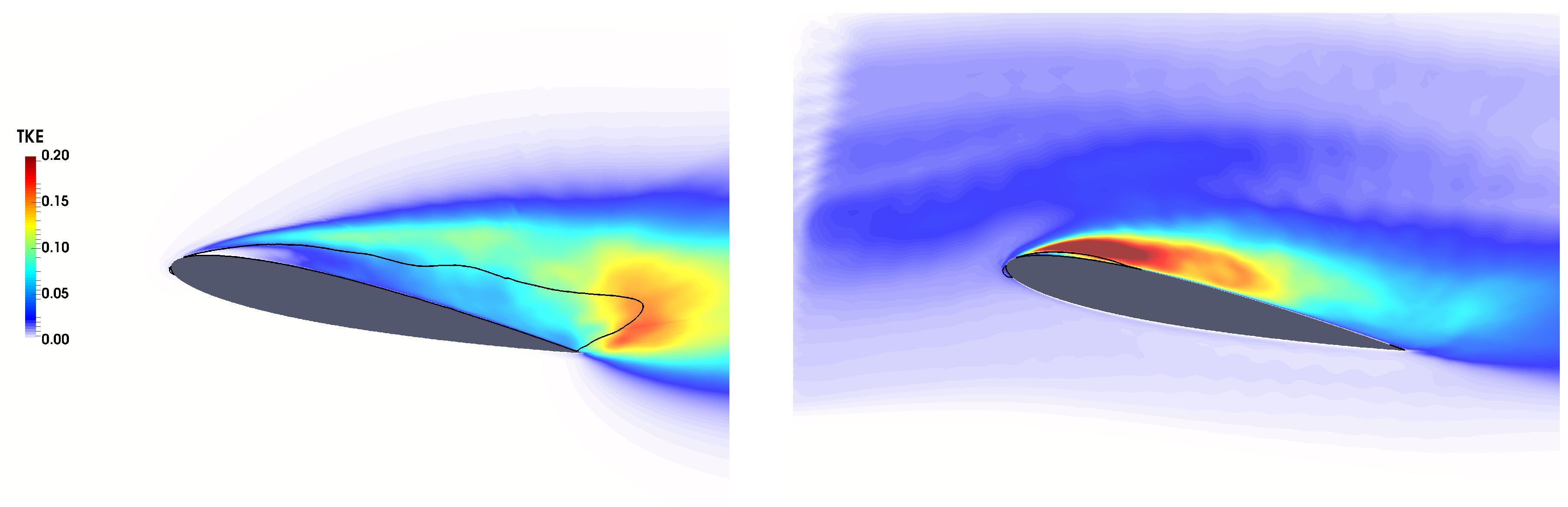
These mechanisms also appear in the averaged flow fields.
Figure 11 shows the mean turbulent kinetic energy. In the laminar freestream case the fluctuations increase along the shear layer and reach the maximum at the end of the reverse flow region above the trailing edge, whereas the turbulence reaches high intensity immediately after separation in turbulent freestream conditions. This turbulence develops close enough to the surface that it causes the flow to reattach soon.
The streamlines in
Figure 12 clearly indicate the locations of separation and reattachment. In the laminar freestream case the secondary recirculation, which has been seen instantaneously, also appears here. Inside the separated region a small system of recirculating vortices appears.
In order to validate the simulation setup results from a DNS of the flow in laminar freestream by Rodriguez et al. [
24] have been used.
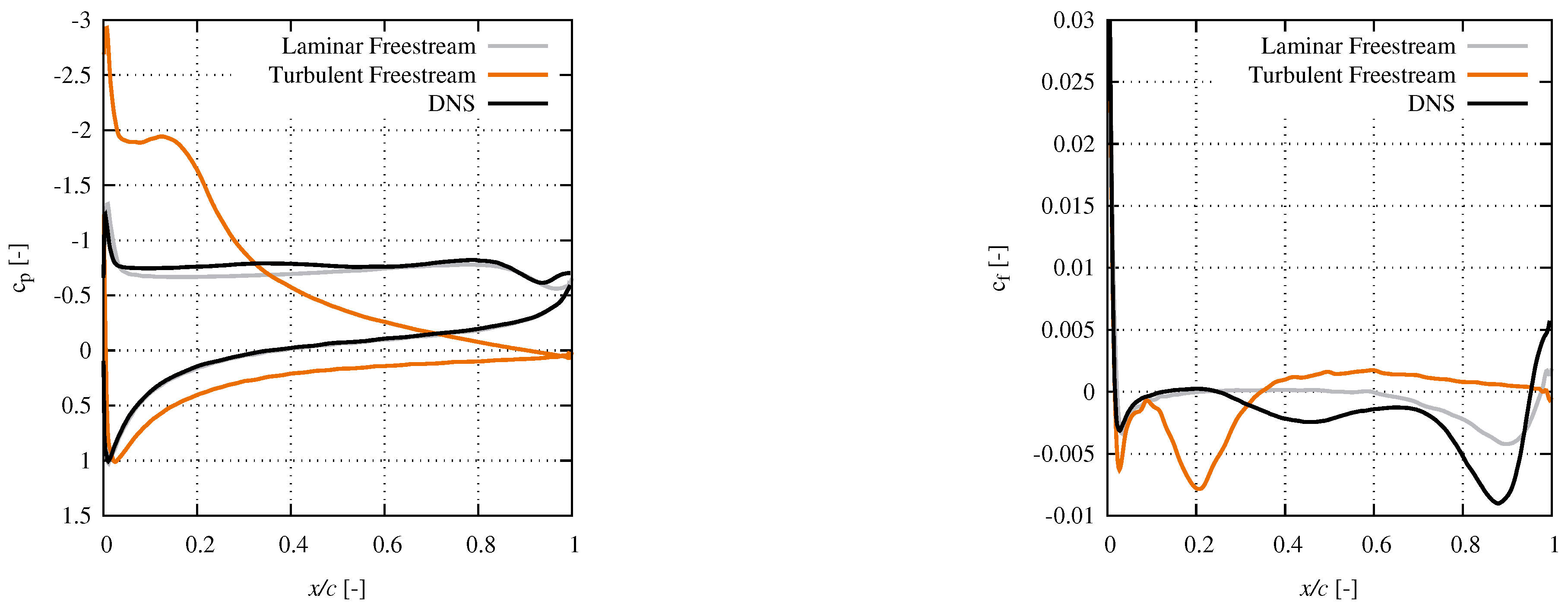
Figure 13 shows the averaged pressure coefficient on both and the friction coefficient on the upper side of the wing. The curves of
for laminar freestream are in very good agreement. On the lower side the curves are almost identical. Some differences appear along the front half of the upper side. They result from slightly different systems of the secondary recirculation between DNS and DDES. In the turbulent freestream case, the presence of a separation bubble in the front is obvious as a plateau forms in the
curve.
In the skin friction plot the locations of the first separation are very similar for all three cases, since this cannot be prevented or delayed by the approaching turbulence at such a high angle of attack. Then both the DDES and the DNS show a secondary recirculation region with positive pointing friction. However, in the DNS only a short range appears whereas in the DDES it is predicted further downstream and lasting for a longer range. The following part of the curves shows the same characteristic with a minimum close to the trailing edge indicating proximity to the recirculation vortex core with higher velocities. The flow reattaches shortly before the trailing edge. This occurs slightly further upstream in the DNS than predicted by the DDES, which is certainly connected with the slight differences in the recirculating flow structure. At turbulent freestream conditions the flow clearly reattaches soon and remains attached until very close to the trailing edge. A very slight separation is indicated around the trailing edge.
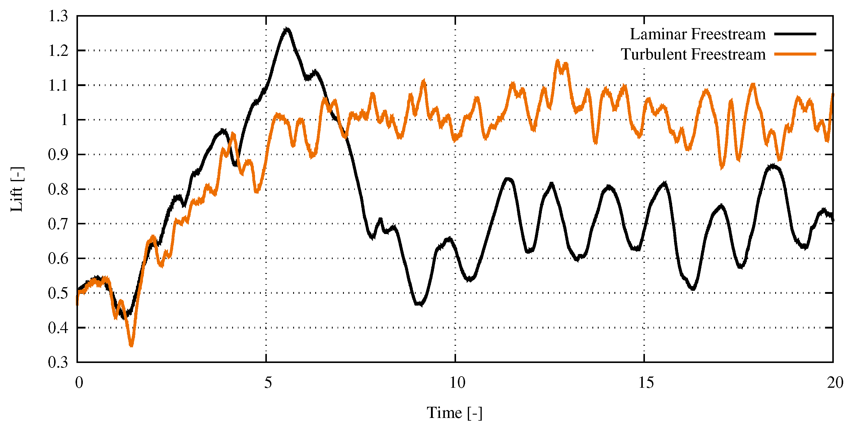
The flow process around the wing in these conditions is a highly unsteady system. Unsteadiness arises not only from the approaching freestream turbulence. The separation process involves vortex shedding and its turbulent breakup into smaller scales. The temporal evolution of the lift coefficient is shown in
Figure 14 for both cases. A quasi steady state is achieved after approximately ten characteristic time units based on chord length and bulk velocity. At laminar freestream one dominant frequency can be seen. It is the frequency of vortex shedding, which causes a periodic oscillation of the lifting force. The Strouhal number based on chord length and bulk velocity (
) is
. Rodriguez et al. state a value of
from their DNS data.
In turbulent conditions the evolution of the lift is determined by several modes. Two of them are dominant, namely and . The latter one is connected with the shear layer vortex shedding, which leads to an oscillation of the separation zone length. The origin of the former one cannot definitively be found based on the available data. It is suspected to arise from the interaction between vortices from the upper and the lower side and requires further investigation.
4. Conclusions and Outlook
A method to introduce turbulence at arbitrary locations within the computational domain by applying volume forces has been supplemented with a mechanism to control the turbulence intensity. The control loop becomes necessary since the turbulence is affected by several phenomena during this process. A set of gain coefficients for the controller terms has been proposed based on simulations of a plain channel to ensure stability of the control loop as well as reasonable response time to achieve a quasi steady state. In order to validate the method synthetic turbulence has been introduced within a farfield-bounded domain without any geometry present. In the resulting fluctuating flow, both turbulence length scale as well as intensity agree with the prescribed target values.
Modifying the momentum equation with a spatially varying volume force implies modifications in the pressure correction equation. The significance of those has been assessed in simulations of a cylinder in freestream turbulence. The cylinder setup also demonstrates, that the controller is capable of scaling the desired fluctuations to an arbitrary intensity. This allows to use one set of fluctuations for a series of simulations with different freestream turbulence intensities.
Finally, the method has been applied to a fully three-dimensional setup of the flow around a NACA0012 airfoil including parallel computing, which requires intercommunication between the processes to exchange the in- and output of the controller. In laminar freestream the flow features full separation, which has been compared and validated with DNS data. The freestream turbulence enhances the formation of shear layer turbulence and thereby causes the flow to reattach. This changes the flow structure above the airfoil entirely. As determined from the oscillations of the lifting force also the dominating frequencies are changed.
The application in separated airfoil and wing flows will be subject to further investigations and was a significant part of the motivation for this work. Laminar separation, particularly at lower angles of attack, is known to be very sensitive to freestream turbulence as shown in other work of the authors [
25,
26]. Further work is required to understand the ongoing phenomena.
Another aspect, which has not been taken into account here, is, that the length scale also is slightly modified in the process. This mainly occurs due to the width of the forcing region, which causes smaller fluctuation spots to be blurred. An approach as proposed in [
20] allows to adapt the length scale dynamically and hence will be followed in the context of controlled freestream turbulence in future work.


