Author Contributions
Conceptualization, C.W., N.F., Y.P.-S., D.G.-V., J.D., F.F. and J.V.R.; methodology, C.W. and J.D.; software, C.W.; formal analysis, C.W., Y.P.-S. and D.G.-V.; investigation, C.W.; data curation, C.W., N.F., Y.P.-S., D.G.-V. and F.F.; writing—original draft preparation, C.W., N.F., Y.P.-S., D.G.-V., J.D., F.F. and J.V.R.; supervision, J.V.R.; project administration, J.R.; funding acquisition, J.R. All authors have read and agreed to the published version of the manuscript.
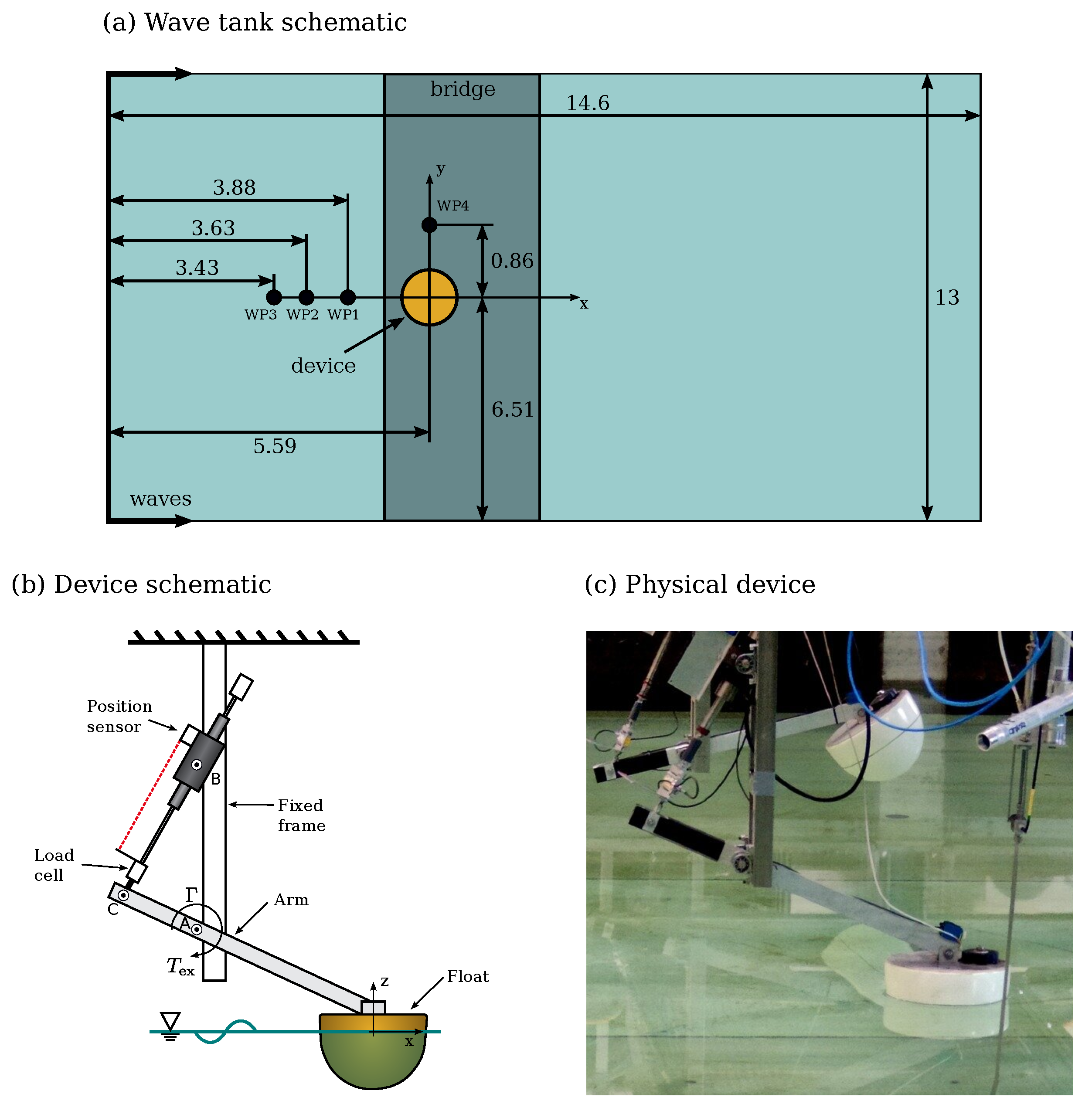
Figure 1.
Schematic (not at scale) of the physical wave tank including the wave probe (WP) positions (all dimensions in [m]) (a) and the device (b). (c) shows a photograph of the physical device.
Figure 1.
Schematic (not at scale) of the physical wave tank including the wave probe (WP) positions (all dimensions in [m]) (a) and the device (b). (c) shows a photograph of the physical device.
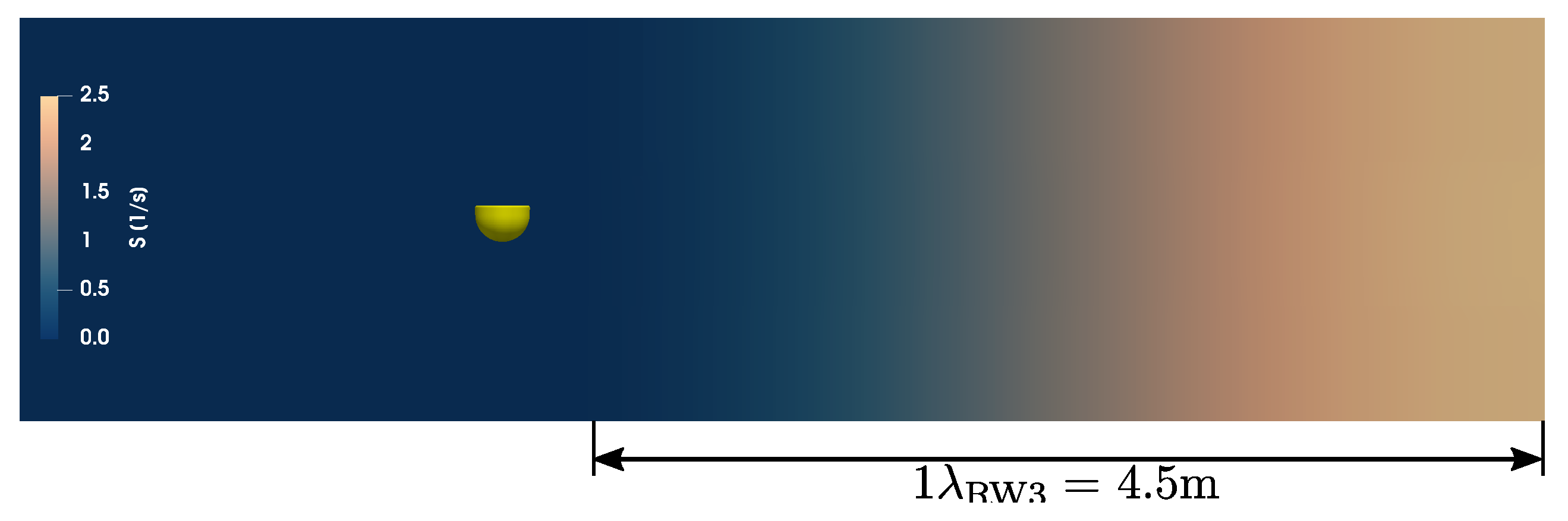
Figure 2.
Side view of the computational domain: Screen shot of the field.
Figure 2.
Side view of the computational domain: Screen shot of the field.
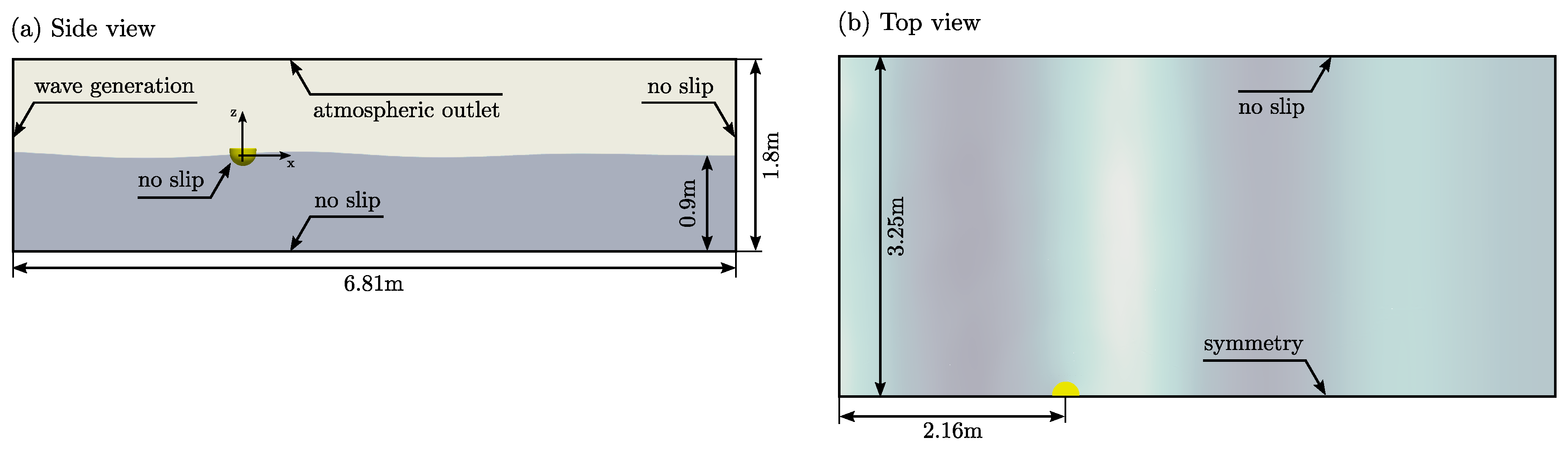
Figure 3.
Schematic of the numerical wave tank: Side view (a) and top view (b).
Figure 3.
Schematic of the numerical wave tank: Side view (a) and top view (b).
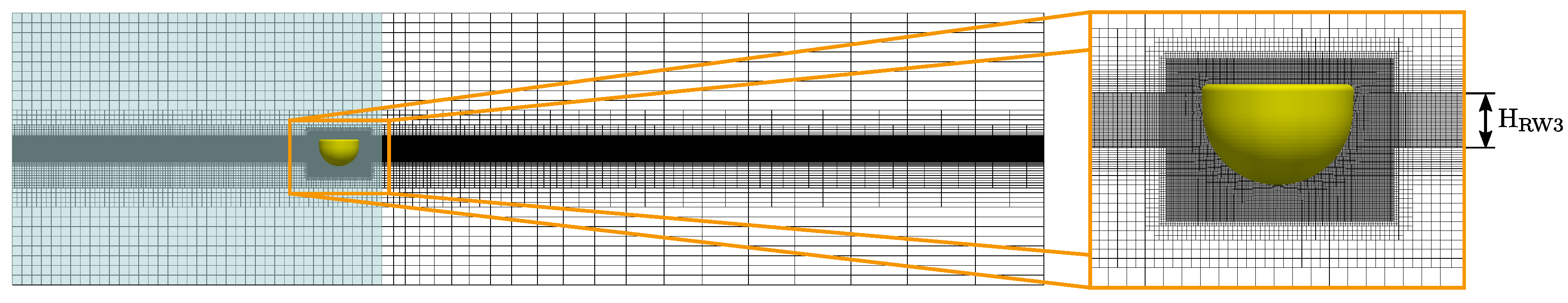
Figure 4.
Screen shot of the computational mesh in the -plane. The simulation zone, in which the damping factor , is highlighted in blue.
Figure 4.
Screen shot of the computational mesh in the -plane. The simulation zone, in which the damping factor , is highlighted in blue.
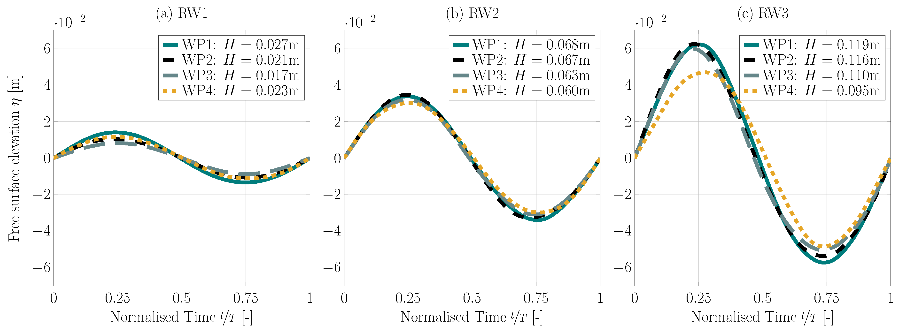
Figure 5.
Phase-averaged free surface elevation, measured at wave probes WP1–WP4 (see
Figure 1), for waves RW1 (
a), RW2 (
b), and RW3 (
c).
Figure 5.
Phase-averaged free surface elevation, measured at wave probes WP1–WP4 (see
Figure 1), for waves RW1 (
a), RW2 (
b), and RW3 (
c).
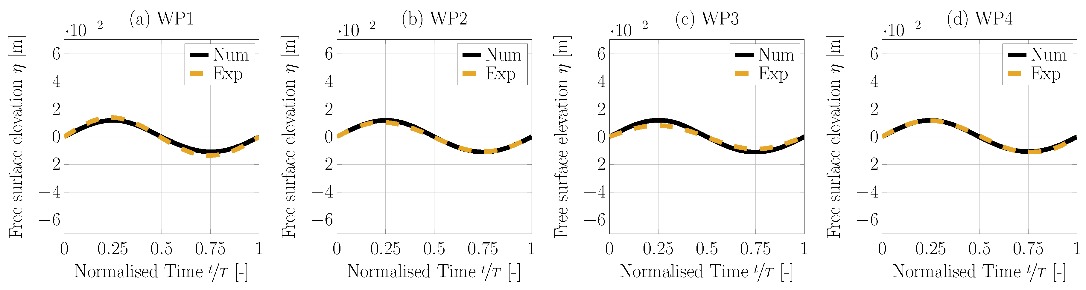
Figure 6.
Phase-averaged free surface elevation, measured at wave probes WP1–WP4 (a–d), for wave RW1.
Figure 6.
Phase-averaged free surface elevation, measured at wave probes WP1–WP4 (a–d), for wave RW1.
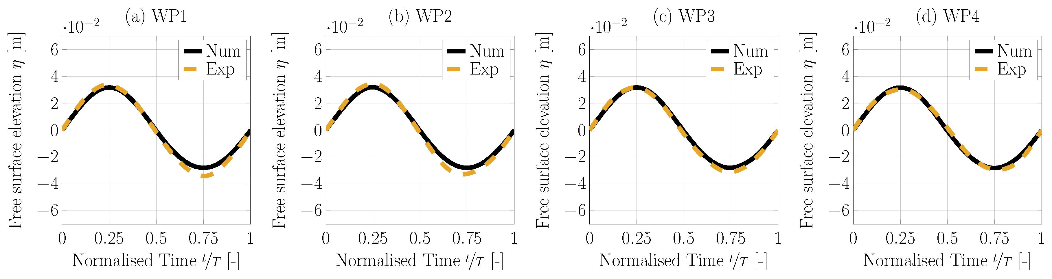
Figure 7.
Phase-averaged free surface elevation, measured at wave probes WP1–WP4 (a–d), for wave RW2.
Figure 7.
Phase-averaged free surface elevation, measured at wave probes WP1–WP4 (a–d), for wave RW2.
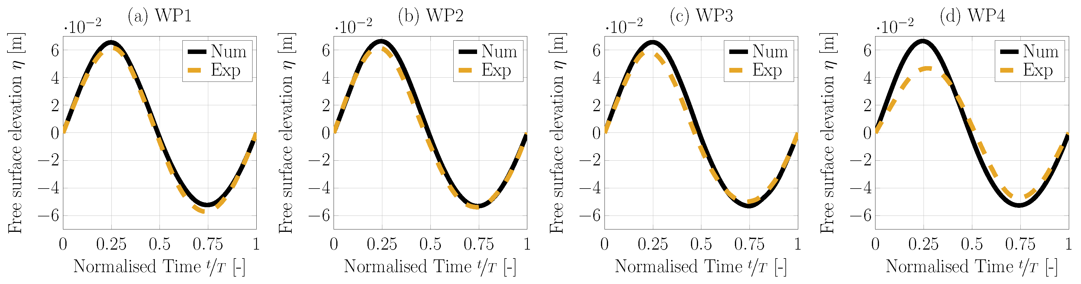
Figure 8.
Phase-averaged free surface elevation, measured at wave probes WP1–WP4 (a–d), for wave RW3.
Figure 8.
Phase-averaged free surface elevation, measured at wave probes WP1–WP4 (a–d), for wave RW3.
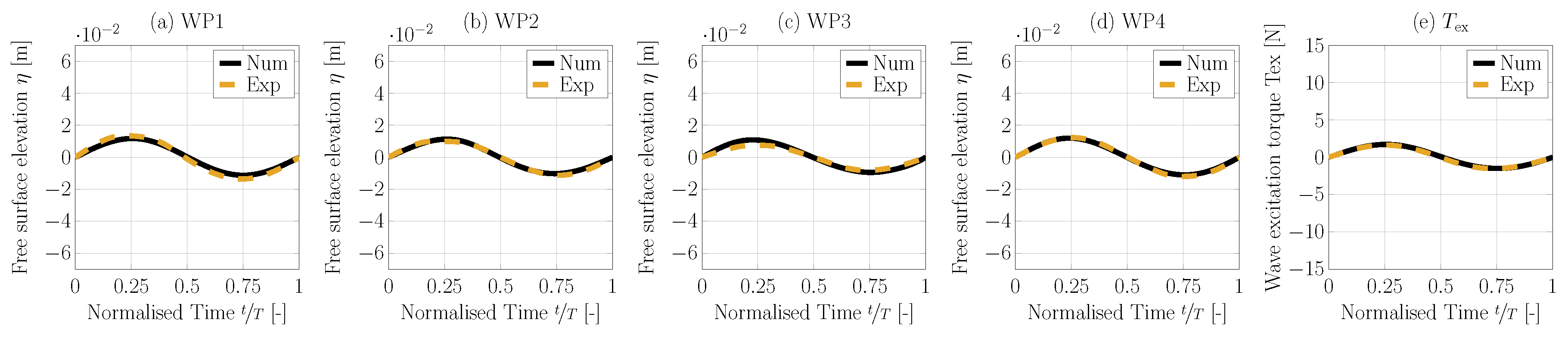
Figure 9.
Phase-averaged free surface elevation, measured at wave probes WP1–WP4 (a–d), and wave excitation torque (e) for wave RW1.
Figure 9.
Phase-averaged free surface elevation, measured at wave probes WP1–WP4 (a–d), and wave excitation torque (e) for wave RW1.
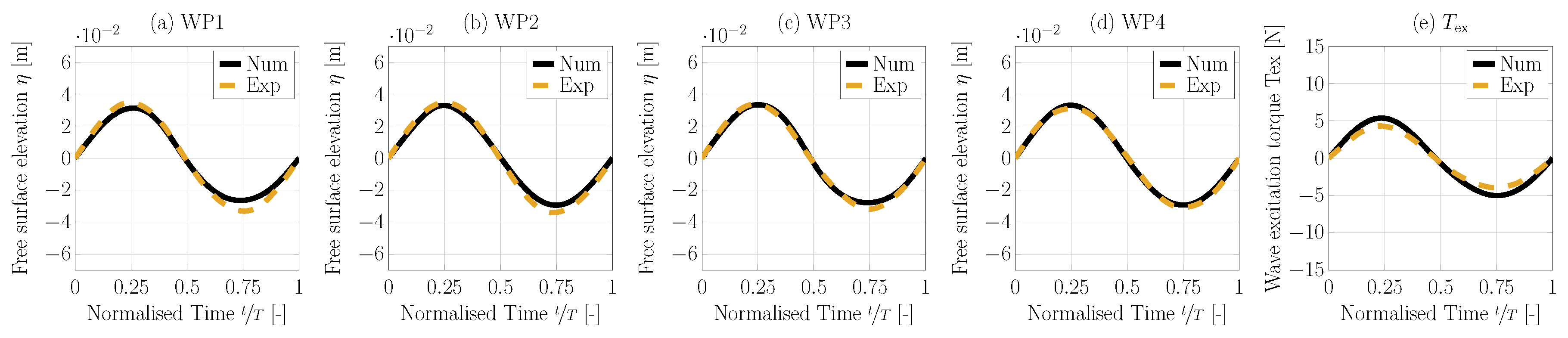
Figure 10.
Phase-averaged free surface elevation, measured at wave probes WP1–WP4 (a–d), and wave excitation torque (e) for wave RW2.
Figure 10.
Phase-averaged free surface elevation, measured at wave probes WP1–WP4 (a–d), and wave excitation torque (e) for wave RW2.
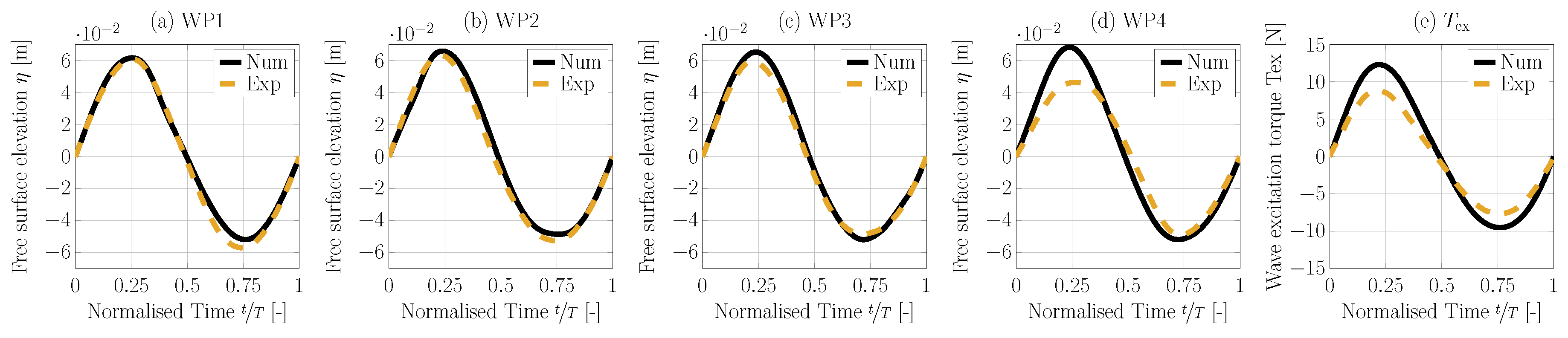
Figure 11.
Phase-averaged free surface elevation, measured at wave probes WP1–WP4 (a–d), and wave excitation torque (e) for wave RW3.
Figure 11.
Phase-averaged free surface elevation, measured at wave probes WP1–WP4 (a–d), and wave excitation torque (e) for wave RW3.
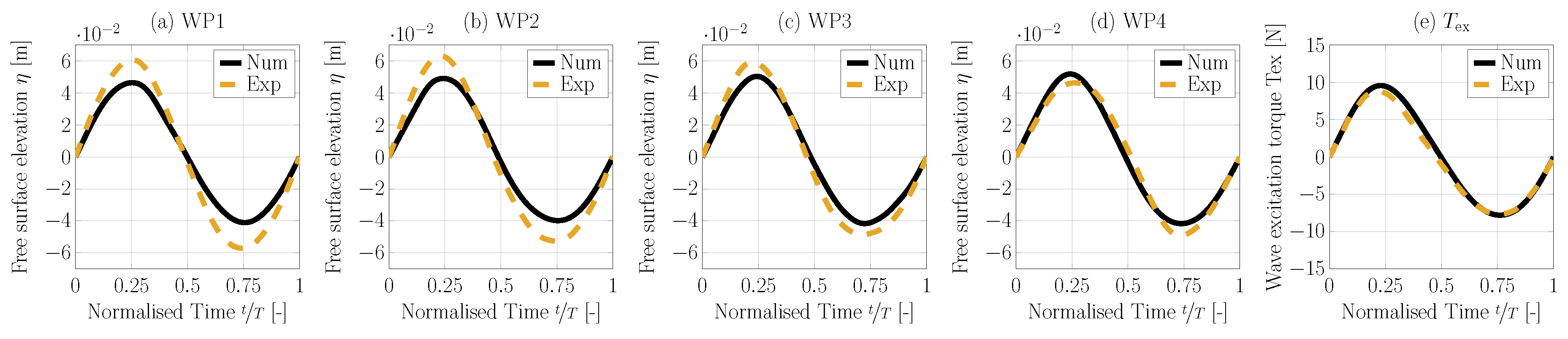
Figure 12.
Phase-averaged free surface elevation, measured at wave probes WP1–WP4 (a–d), and wave excitation torque (e) for wave RW3*.
Figure 12.
Phase-averaged free surface elevation, measured at wave probes WP1–WP4 (a–d), and wave excitation torque (e) for wave RW3*.
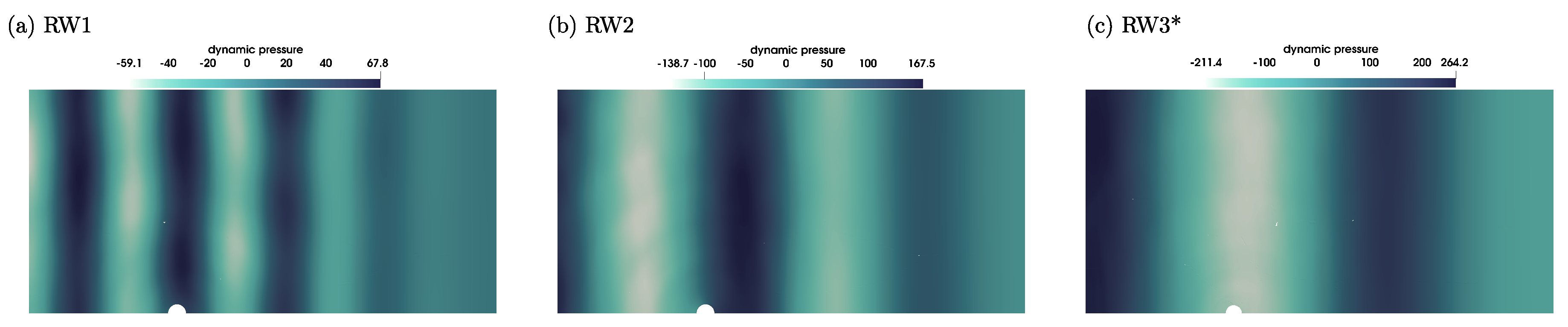
Figure 13.
Screen shot of the dynamic pressure for waves RW1 (a), RW2 (b), and RW3* (c).
Figure 13.
Screen shot of the dynamic pressure for waves RW1 (a), RW2 (b), and RW3* (c).
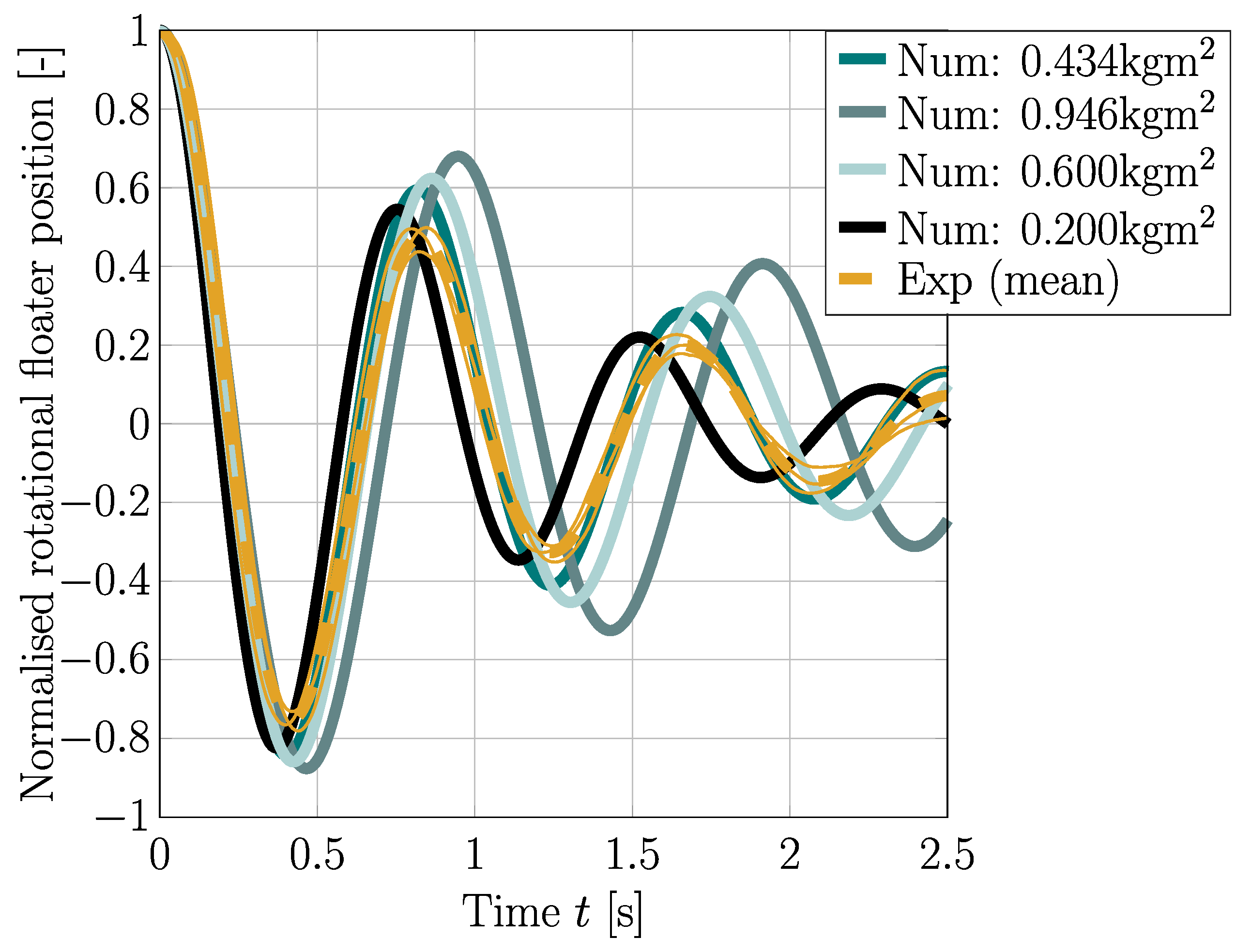
Figure 14.
Time trace of the normalised floater position during the free decay test.
Figure 14.
Time trace of the normalised floater position during the free decay test.
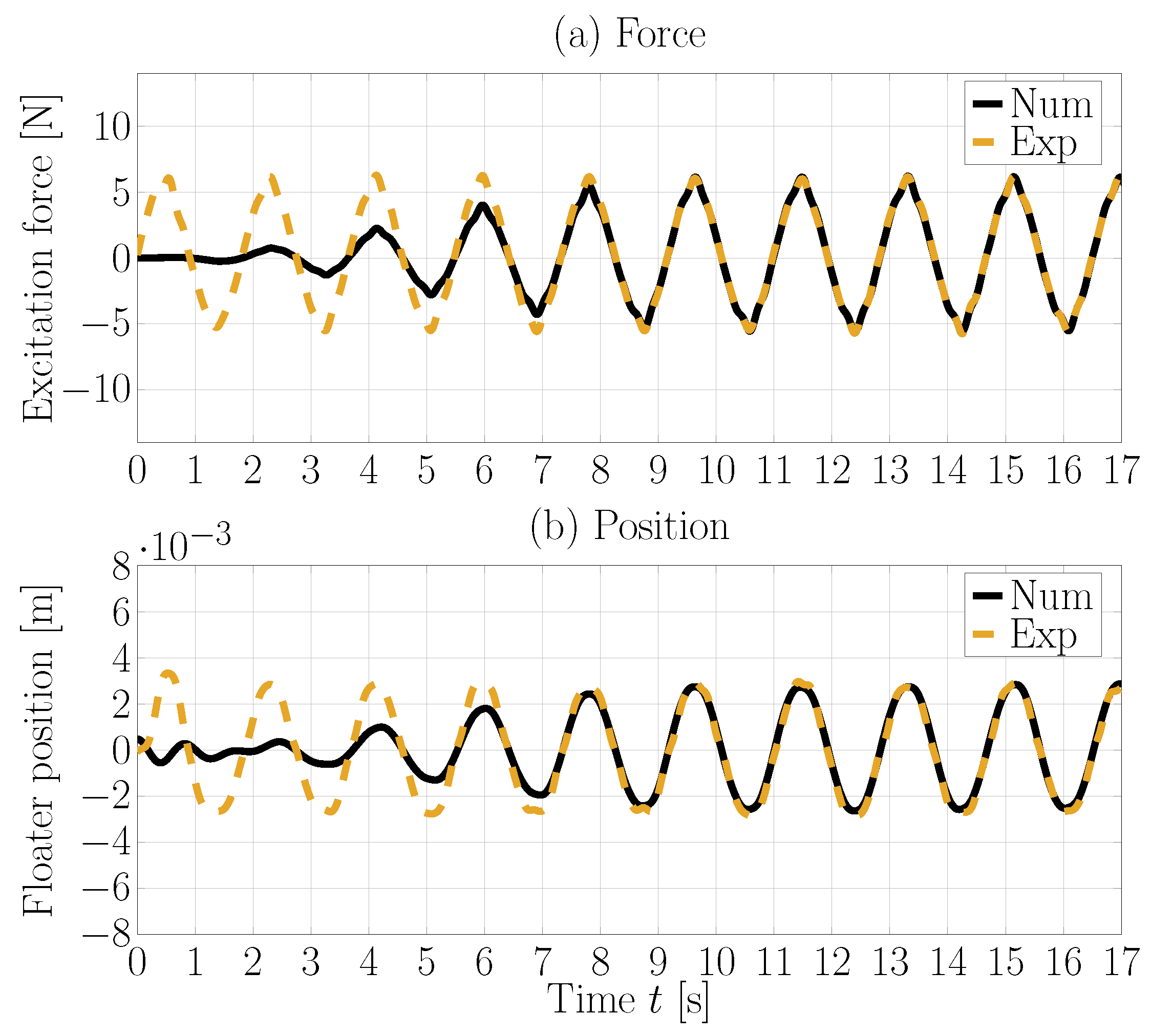
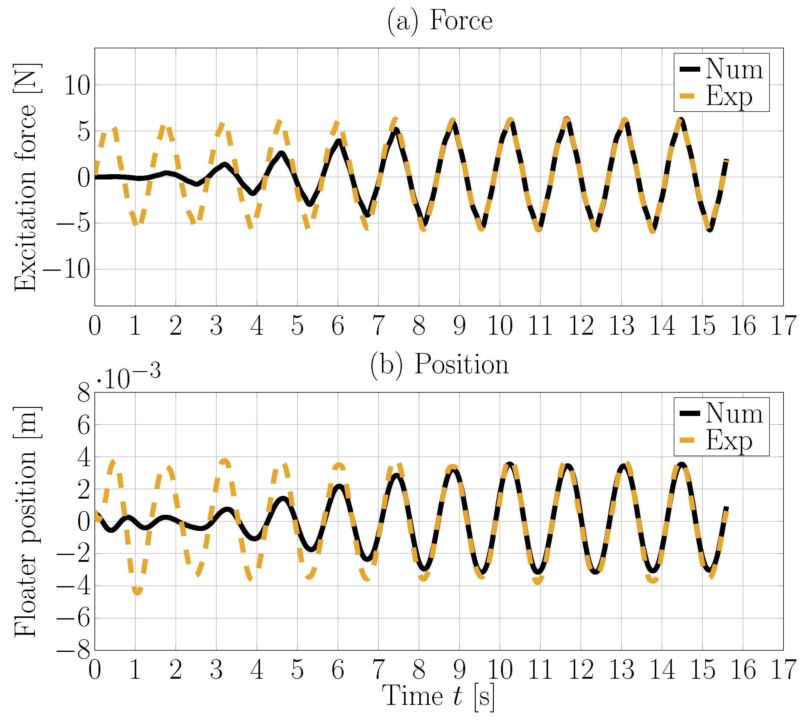
Figure 15.
Time trace of the single-frequency (0.54 Hz) excitation force (a) and the floater position (b).
Figure 15.
Time trace of the single-frequency (0.54 Hz) excitation force (a) and the floater position (b).
Figure 16.
Time trace of the single-frequency (0.54 Hz) excitation force (a) and the floater position (b).
Figure 16.
Time trace of the single-frequency (0.54 Hz) excitation force (a) and the floater position (b).
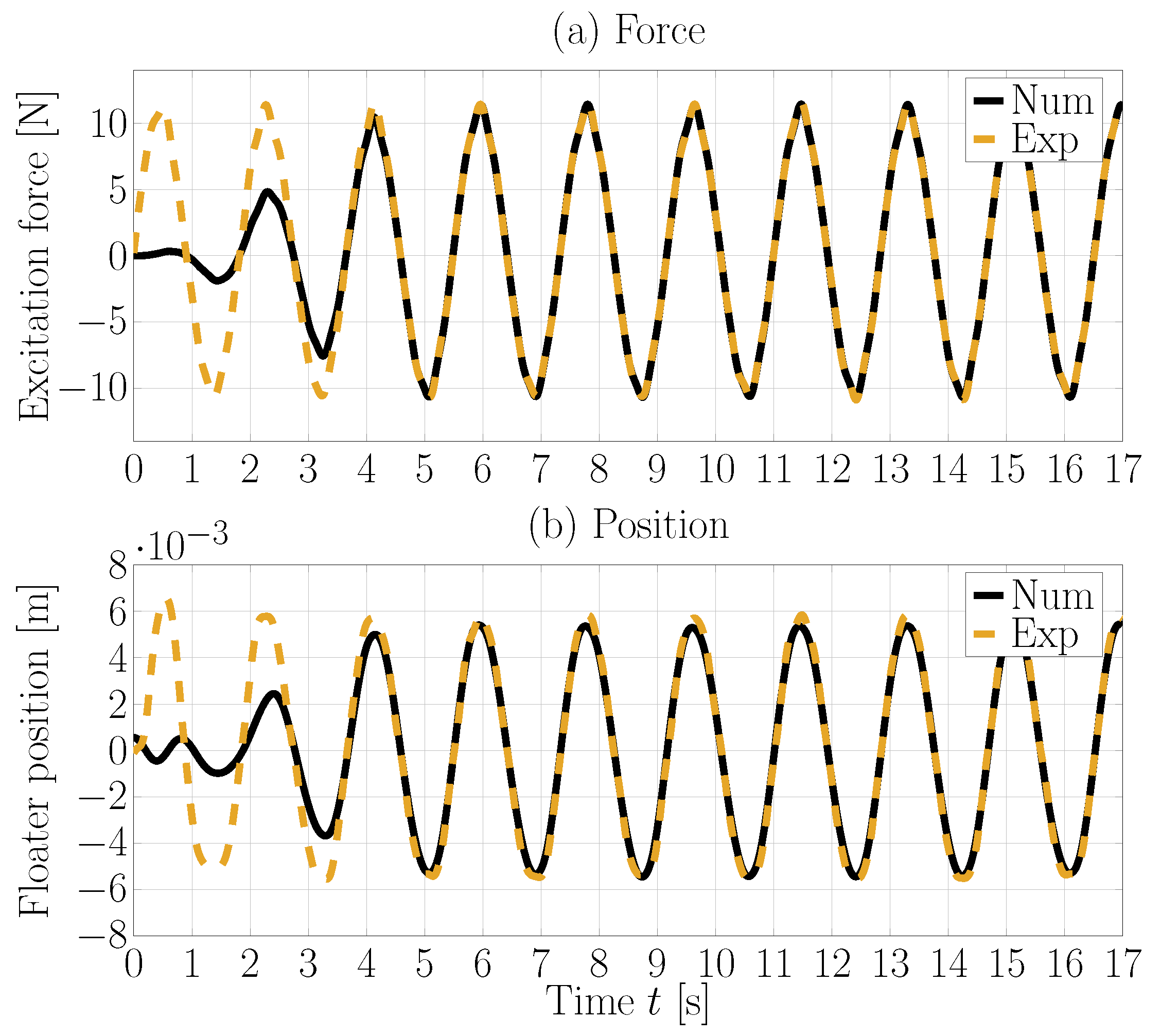
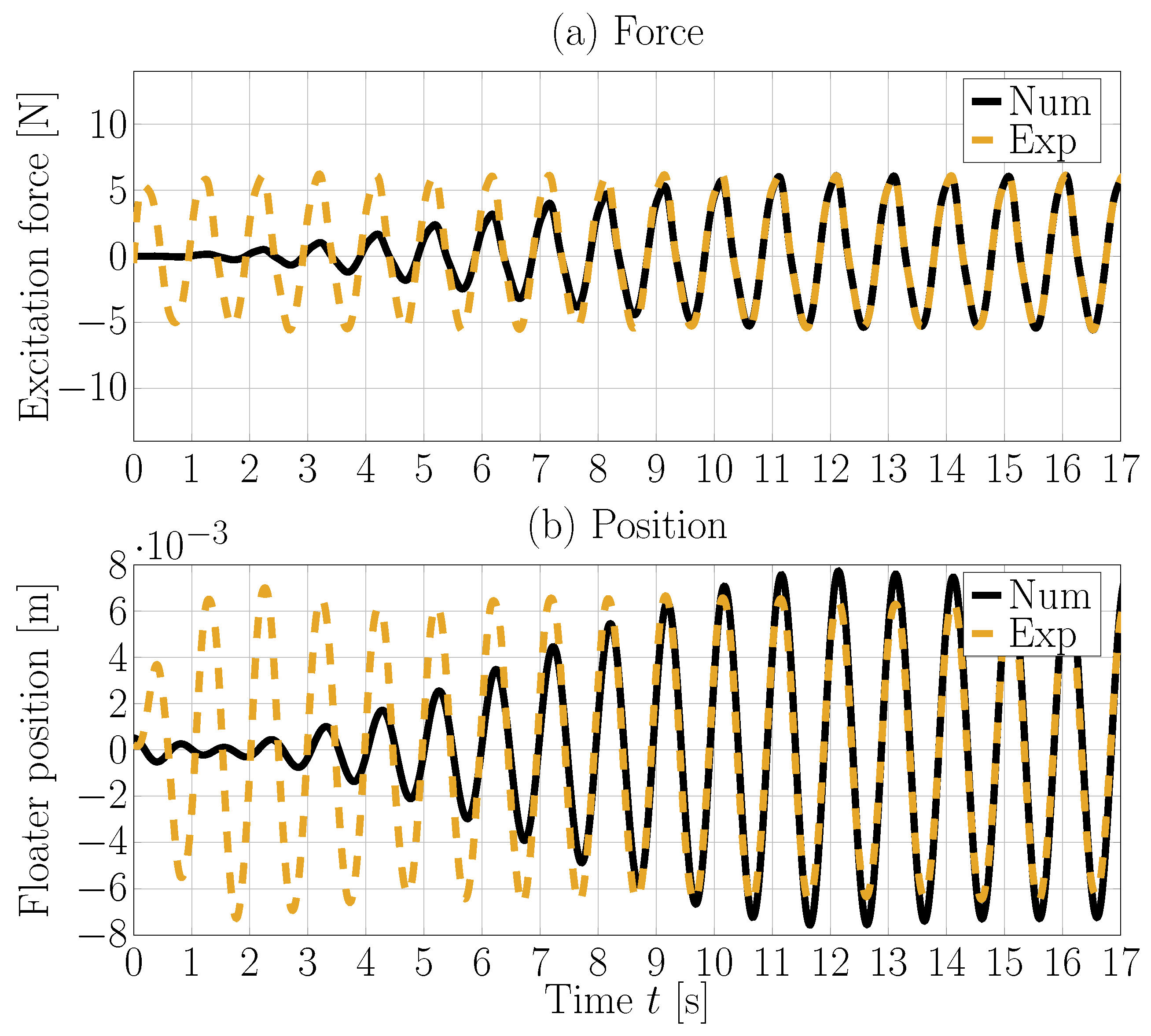
Figure 17.
Time trace of the single-frequency (0.71 Hz) excitation force (a) and the floater position (b).
Figure 17.
Time trace of the single-frequency (0.71 Hz) excitation force (a) and the floater position (b).
Figure 18.
Time trace of the single-frequency (1.01 Hz) excitation force (a) and the floater position (b).
Figure 18.
Time trace of the single-frequency (1.01 Hz) excitation force (a) and the floater position (b).
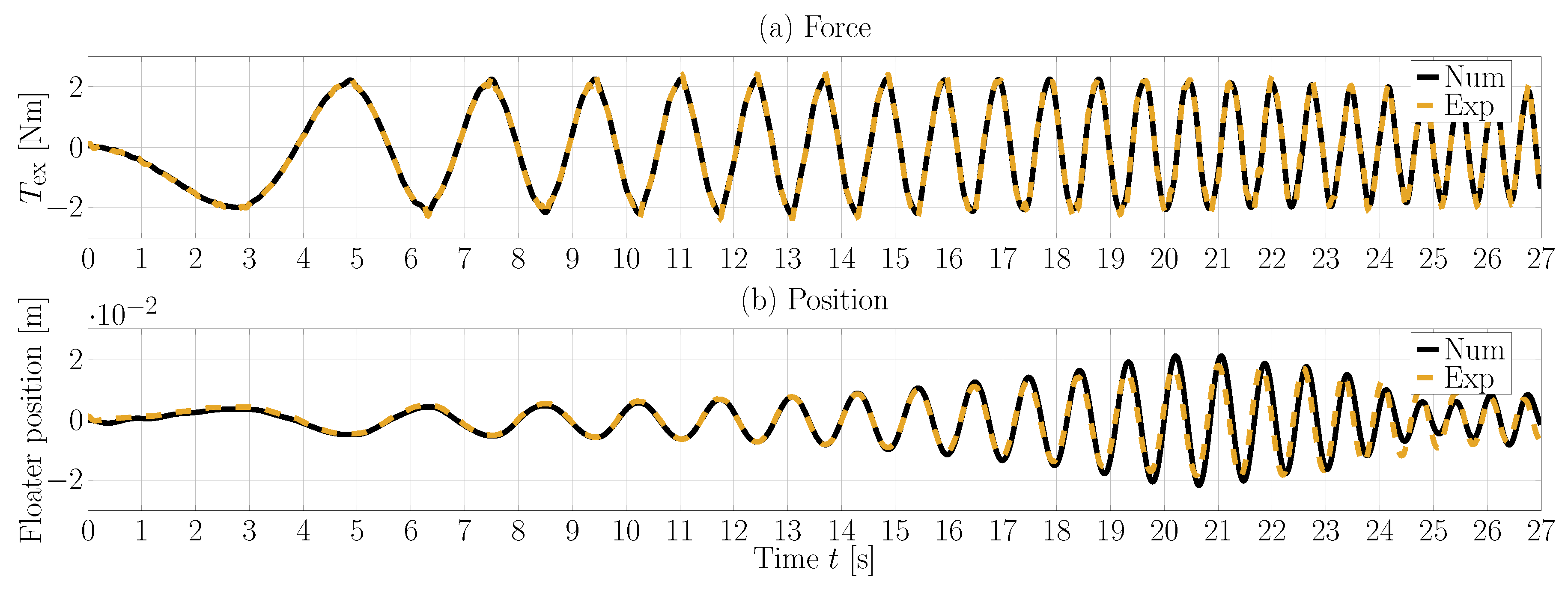
Figure 19.
Time trace of the multi-frequency excitation torque (a) and the floater position (b).
Figure 19.
Time trace of the multi-frequency excitation torque (a) and the floater position (b).
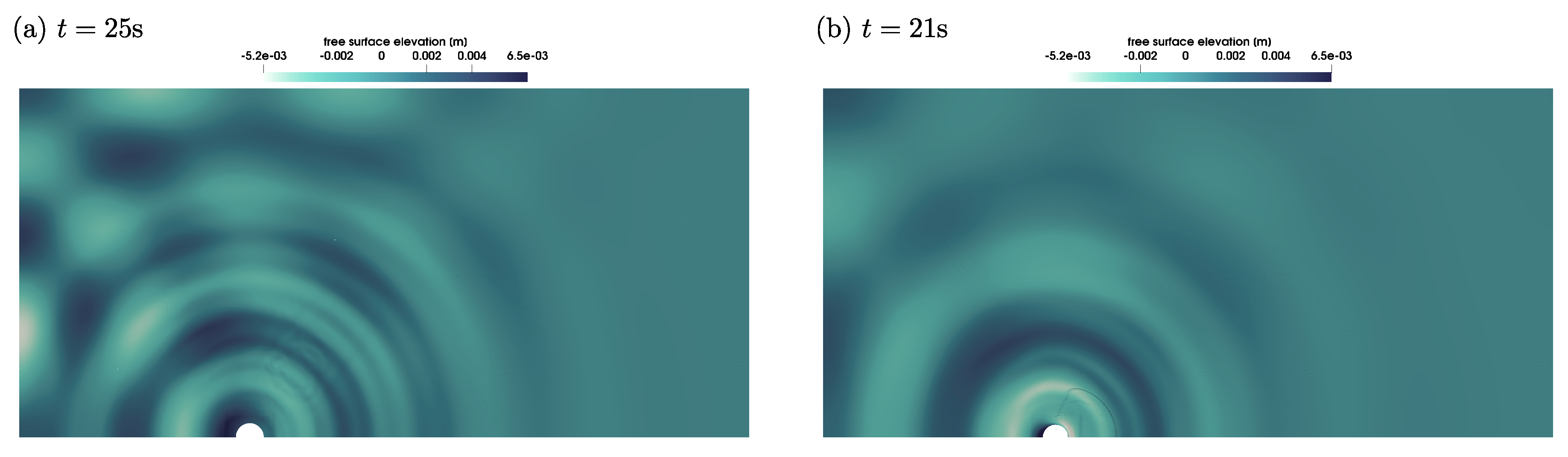
Figure 20.
Screen shots of the free surface during the multi-frequency forced oscillation test at s (a) s (b).
Figure 20.
Screen shots of the free surface during the multi-frequency forced oscillation test at s (a) s (b).
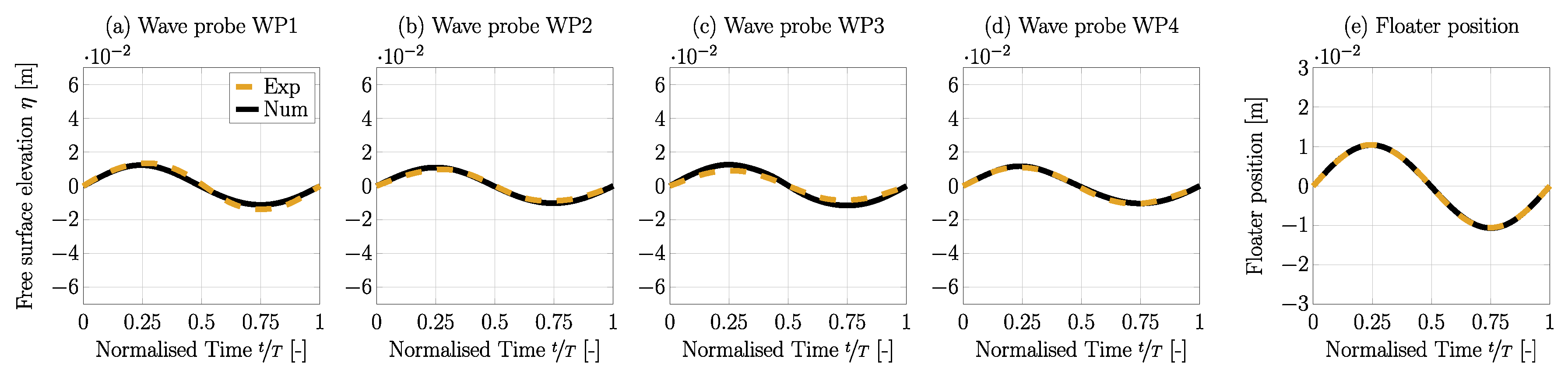
Figure 21.
Phase-averaged free surface elevation, measured at wave probes WP1–WP4 (a–d), and floater position (e) for wave RW1.
Figure 21.
Phase-averaged free surface elevation, measured at wave probes WP1–WP4 (a–d), and floater position (e) for wave RW1.
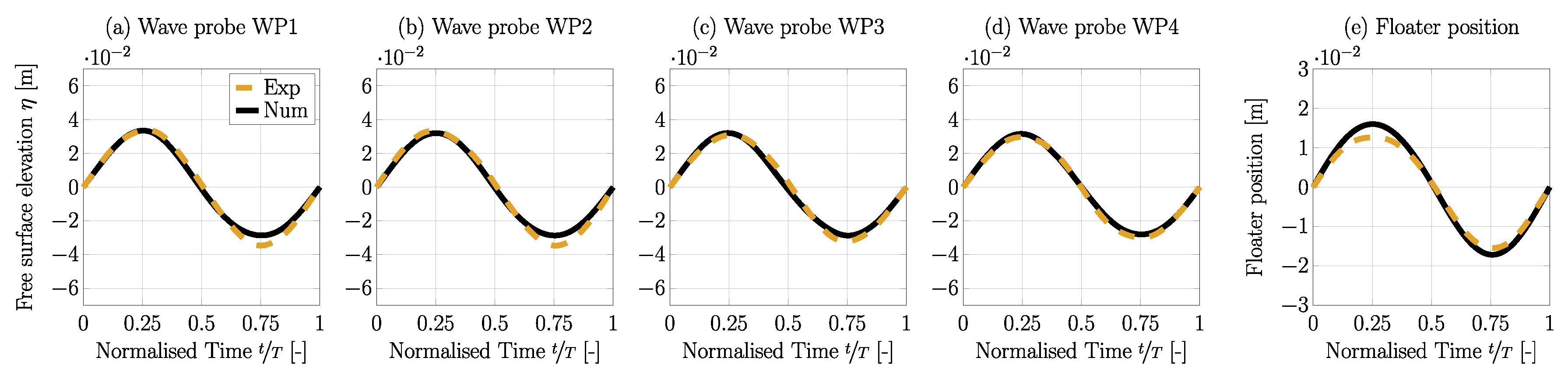
Figure 22.
Phase-averaged free surface elevation, measured at wave probes WP1–WP4 (a–d), and floater position (e) for wave RW2.
Figure 22.
Phase-averaged free surface elevation, measured at wave probes WP1–WP4 (a–d), and floater position (e) for wave RW2.
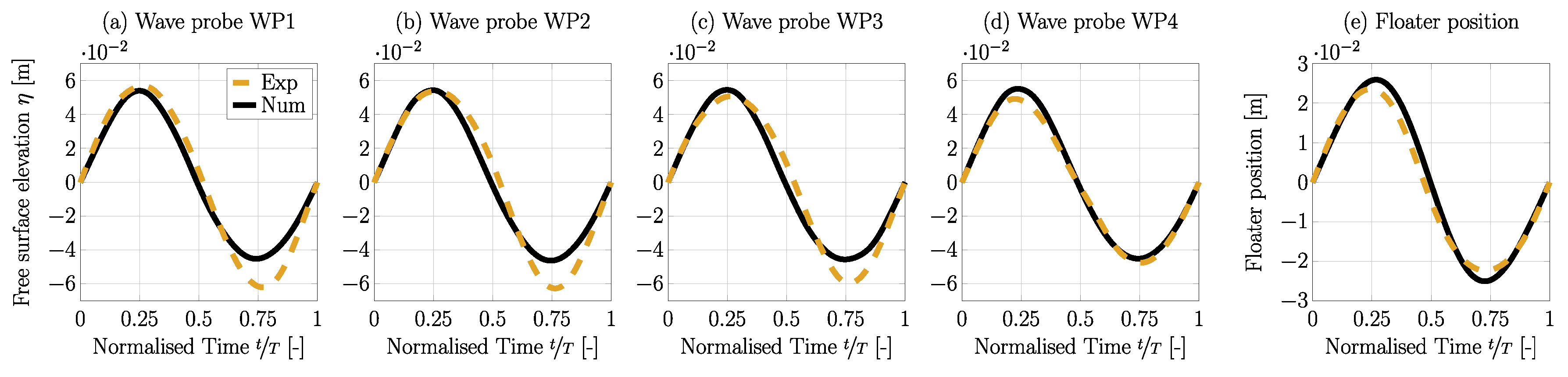
Figure 23.
Phase-averaged free surface elevation, measured at wave probes WP1–WP4 (a–d), and floater position (e) for wave RW3*.
Figure 23.
Phase-averaged free surface elevation, measured at wave probes WP1–WP4 (a–d), and floater position (e) for wave RW3*.
Table 1.
Physical properties of the 1/20th scale Wavestar model. All measurements taken from [
11] are printed in bold.
Table 1.
Physical properties of the 1/20th scale Wavestar model. All measurements taken from [
11] are printed in bold.
| Hinge A: | | |
| x | | |
| y | | |
| z | | |
| Hinge B: | | |
| x | | |
| y | | |
| z | | |
| Hinge C: | | |
| x | | |
| y | | |
| z | | |
| Centre of Mass (CoM): | | |
| x | | |
| y | | |
| z | | |
| Mass (Float & Arm) | | |
| Inertia (Float & Arm) | | |
| Floater diameter (at SWL) | | |
| Submergence (in equilibrium) | | |
| Water depth d | | |
Table 2.
Characteristics of the regular waves.
Table 2.
Characteristics of the regular waves.
| Wave ID | | T | f | | |
|---|
| RW1 | 0.021 m | 0.99 s | 1.01 Hz | 1.56 m | 0.0135 |
| RW2 | 0.063 m | 1.41 s | 0.71 Hz | 2.93 m | 0.0215 |
| RW3 | 0.115 m | 1.84 s | 0.54 Hz | 4.50 m | 0.0256 |
Table 3.
Wave height, H, and the mean standard deviation, , normalised against the mean wave height, from the experimental data for waves RW1–RW3.
Table 3.
Wave height, H, and the mean standard deviation, , normalised against the mean wave height, from the experimental data for waves RW1–RW3.
| RW1 | WP1 | WP2 | WP3 | WP4 |
|---|
| H [m] | 0.027 | 0.021 | 0.017 | 0.023 |
| [%] | 0.56 | 0.68 | 0.76 | 0.53 |
| RW2 | | | | |
| H [m] | 0.068 | 0.067 | 0.063 | 0.060 |
| [%] | 0.66 | 0.58 | 0.48 | 0.31 |
| RW3 | | | | |
| H [m] | 0.119 | 0.116 | 0.110 | 0.095 |
| [%] | 0.70 | 0.59 | 0.72 | 0.48 |
Table 4.
nRMSD between the experimental and numerical free surface elevation, for waves RW1–RW3.
Table 4.
nRMSD between the experimental and numerical free surface elevation, for waves RW1–RW3.
| RW1 | WP1 | WP2 | WP3 | WP4 |
|---|
| nRMSD [%] | 8.31 | 3.86 | 10.70 | 2.27 |
| RW2 | | | | |
| nRMSD [%] | 4.66 | 4.78 | 2.82 | 2.42 |
| RW3 | | | | |
| nRMSD [%] | 2.87 | 3.75 | 5.00 | 9.26 |
Table 5.
nRMSD between the experimental and numerical free surface elevation and excitation torque for waves RW1–RW3.
Table 5.
nRMSD between the experimental and numerical free surface elevation and excitation torque for waves RW1–RW3.
| RW1 | WP1 | WP2 | WP3 | WP4 | |
|---|
| nRMSD [%] | 8.49 | 3.83 | 8.42 | 3.04 | 2.70 |
| RW2 | | | | | |
| nRMSD [%] | 5.56 | 4.45 | 2.82 | 1.93 | 9.32 |
| RW3 (H = 0.115 m) | | | | | |
| nRMSD [%] | 3.17 | 3.77 | 3.42 | 9.76 | 12.48 |
| RW3* (H = 0.095 m) | | | | | |
| nRMSD [%] | 12.14 | 10.97 | 7.70 | 5.34 | 4.31 |
Table 6.
nRMSD between the experimental and numerical free surface elevation and floater position for waves RW1–RW3*.
Table 6.
nRMSD between the experimental and numerical free surface elevation and floater position for waves RW1–RW3*.
| RW1 | WP1 | WP2 | WP3 | WP4 | Floater Position |
|---|
| nRMSD [%] | 8.91 | 4.42 | 10.99 | 2.56 | 0.32 |
| RW2 | | | | | |
| nRMSD [%] | 4.45 | 4.56 | 3.73 | 2.28 | 6.06 |
| RW3* | | | | | |
| nRMSD [%] | 9.95 | 9.75 | 8.56 | 3.89 | 5.54 |

 ,
, 


