Abstract
A variety of devices and concepts have been proposed and thoroughly investigated for the exploitation of renewable wave energy. Many of the devices operate in nearshore and coastal regions, and thus, variable bathymetry could have significant effects on their performance. In particular, Oscillating Wave Surge Converters (OWSCs) exploit the horizontal motion of water waves interacting with the flap of the device. In this work, a Boundary Element Method (BEM) is developed, and applied to the investigation of variable bathymetry effects on the performance of a simplified 2D model of a surge-type wave energy converter excited by harmonic incident waves. Numerical results, illustrating the effects of depth variation in conjunction with other parameters, like inertia and power-take-off, on the performance of the device, are presented. Finally, a comparative evaluation of the present simplified surge-type WEC model and point absorbers is presented for a case study in a selected coastal site on the Greek nearshore area, characterized by relatively increased wave energy potential.
1. Introduction
During the last period, marine renewables have been the subject of intensive research worldwide, both by the industry and the academic community. More specifically, water waves provide a sustainable and widely available source of energy, which could be used to enhance the fraction of green energy in the global production. A great variety of Wave Energy Converters (WECs), devices and concepts based on oscillating systems have been proposed (e.g., see [1,2]), many of which have been also experimentally tested and are currently successfully contributing to the energy grid. In particular, Oscillating Wave Surge Converters (OWSCs) exploit the horizontal motion of water waves, interacting with the flap of the device, to generate renewable electricity [3,4,5]. A typical OWSC consists of a frame on which a shaft is mounted and a flap which performs angular oscillations, with the aforementioned shaft being the center of rotation. The frame is fastened at the seabed (or rests on an auxiliary structure at a lower depth) and is fitted with a hydraulic generator. Fluid is compressed into the hydraulic generator due to the angular oscillation, and the pressure is then transferred, by means of an appropriate pipeline system, to a hydroelectric power station to generate electricity. Methods for the analytical and computational modelling of such wave energy systems have been presented by various authors (e.g., see [6]).
As regards the devices that operate in nearshore and coastal regions, effects caused on their response due to finite water depth bathymetric inhomogeneities could be significant, and need to be considered; e.g., see [7]. This has been illustrated in the case of point absorbers operating in variable bathymetry regions, for which models based on the Boundary Element Method (BEM) have been developed, e.g., [8,9], where it is shown that bottom slope and curvature could have an effect on the performance of the systems, especially in shallow water conditions.
In this work, a novel BEM scheme is developed and applied to the investigation of depth inhomogeneity effects on the performance of surge-type wave energy converters excited by harmonic incident waves, studied in the context of linearized water-wave theory. For simplicity, we restrict ourselves to a two-dimensional flap-type configuration and normally incident waves. Although the present simplified 2D BEM model does not accurately treat the 3D effects of an OWSC like the Oyster device, as extensively discussed by Renzi et al. [4], it still provides useful information, especially as concerns the variable bathymetry effects on the performance of the device. The terminator-type model is studied in two dimensions, where the flap of the device is aligned perpendicular to the incident wave direction (e.g., see [4]). As well as the standard absorbing–radiating model depicted in Figure 1a, which includes additional effects due to wave transmission in the downwave region behind the flap-board, an absorbing–reflecting model, shown in Figure 1b, is also considered. The present numerical method is first validated by comparison to an analytical solution, derived in constant water depth and presented in detail in the Appendix A. Although the latter absorbing–reflecting configuration could be represented by the former absorbing–radiating model, with appropriate adjustment of the Power Take Off (PTO) parameters to achieve zero transmitted wave, still it is considered here as a special case, and used for the additional validation of the developed BEM model.
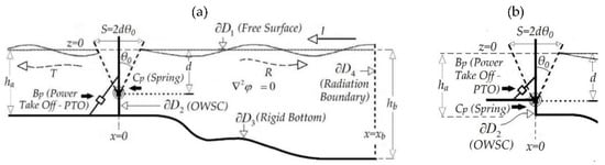
Figure 1.
Simplified 2D model of terminator-type Oscillating Wave Surge Converters (OWSC) (a) standard absorbing–radiating model including additional radiation effects in the downwave region behind the flap-board, and (b) the special case of an absorbing–reflecting model. Definition of the variable bathymetry domain and decomposition of the boundary into four sections.
Subsequently, the 2D BEM model is applied to illustrate the effects of depth variation, including sloping and corrugated seabeds, in conjunction with other parameters, like inertia and power-take-off coefficients. Results are used to show and discuss the response of the considered system in inhomogeneous regions. Although nonlinearity associated with large wave heights, wave breaking and viscous fluid effects are significant, a linear model could still provide useful information for the performance and optimization of the devices, as well as estimates of power performance measures that can be derived (e.g., see [10]).
In the last section of this work, a case study is presented providing useful data concerning the available wave energy at a nearshore/coastal site with relatively increased potential in the Aegean Sea. Using the latter data, a comparative evaluation of the present simplified surge-type WEC model and point absorbers is presented, deriving power performance measures that can be further exploited to levelized energy cost analysis. A discussion concerning the validity and shortcomings of the present simplified analysis is also included, especially as concerns the three dimensional and real fluid effects, which will be treated in future work.
2. Hydrodynamic Analysis of A Two-dimensional Flap-Type Model in Variable Bathymetry
In this work, a simplified two-dimensional BEM model is presented for the hydrodynamic analysis of a flap-type device, in the case of normally incident waves in variable bathymetry, shown in Figure 1, in the context of linearized wave theory. In all cases, a zero-thickness flap boundary is considered.
Without loss of generality, a left horizontally semi-infinite domain is considered, (see Figure 1), starting from xa = 0 where the flap-type device is located. In order to study variable bathymetry effects on the performance of the two-dimensional flap-type model (2dOSWC), a low-order Boundary Element Method (BEM) is developed (e.g., see [11]). The method is first validated by comparison between the numerical and the analytical results in constant water depth, for which an analytical solution is described in Appendix A. Subsequently, the numerical model is used in order to show and discuss the variable bathymetry effects.
The present panel method is based on the approximation of the boundary by linear elements/panels carrying simple source–sink distributions. We assume harmonic time dependence in the form , and the complex wave potential is represented by:
where denotes the fundamental solution of the Laplace Equation in the two-dimensional space, x(x,z) is a general field point in the domain, while x0(x,z) indicates the singularity point, and denotes the boundary of the domain decomposed into four sections, as presented in Figure 1: the free surface , the device part , the seabed and the vertical interface serving as an incidence–radiation boundary.
The solution to the potential flow problem is obtained by discretizing the boundary geometry into elements , in conjunction with the approximation of the unknown source–sink function—which is assumed to be piecewise constant on each element—and enforcing the boundary conditions on the control points of each boundary’s part (defined as the elements’ midpoints), from which the source–sink singularity strength on each element is determined. Under the assumption that the variable bathymetry domain, shown in Figure 1, ends in a semi-infinite constant-depth strip, and that the interface located at , lies well within the constant-depth region, where the effects of evanescent modes have died out, the complex wave potential consisting of the incident and reflected wave can be expressed by considering the propagating mode only, as follows:
where , with denoting the acceleration of gravity and H the incident wave height. Moreover, R is the reflection coefficient, the function and the wavenumber of the incident-reflected wave is obtained from the dispersion relation formulated at the radiation boundary depth :
Using Equation (2), the horizontal wave velocity is calculated by the partial x-derivative of the normalized complex wave potential φ at , as follows:
The vertical eigenfunctions are derived from the solution of the Sturm–Liouville problem, to which the Laplace equation is reduced in the constant depth strip The latter are , with the corresponding parameters obtained as the imaginary roots of Equation (3). By projecting the two members of Equation (2) in the above orthogonal vertical basis we obtain:
where . Consequently, Equation (5) can be solved for R, providing an expression of the reflection coefficient as a function of the complex wave potential in the water column at :
Substitution of the reflection coefficient’s expression in Equation (4) results in the following radiation condition, that applies on the interface (radiation boundary):
where denotes the normal derivative of the wave potential on the boundary, with respect to the outward directed unit normal vector . The boundary conditions that apply on the other three sections of the boundary are:
where the functions and represent the oscillatory normal component of the velocity due to the flap motion, and are simply zero on the wall below the pivot point of the OWSC, located at z = −d (see Figure 1).
2.1. Mesh Generation
The boundary is discretized by a closed polygonal line, which is formed by distributing nodes across its length. In particular, the free surface nodes are determined by specifying a number of nodes per characteristic wavelength in the domain that is usually larger than 30–40. Next, the free surface nodes are redefined, using a cosine spacing, to allow them to be more densely arranged approaching the corners of the domain. The z-coordinates of the free surface’s nodes are equal to , where denotes the number of elements on the free surface. The bottom boundary is discretized accordingly, with the z-coordinates set equal to , where is the number of elements on the seabed, is the depth function, and are the number of elements on the vertical boundaries (OWSC and radiation boundary, respectively). The node spacing is finer on the horizontal boundaries near the corners of the domain, while it is uniform on the vertical sides. The latter is selected to match the fine spacing of the horizontal sides at the corners. Based on the above discretization, the total number of elements is .
2.2. Discrete BEM Model
By assuming unit source–sink singularity strengths on each element, the induced potential and velocity matrices , from each element to each collocation point, are analytically calculated; see [11]. Using the latter quantities in the boundary conditions, the influence matrix of the discrete system is obtained, as explained in more detail in the sequel. By denoting with the strength of the source/sink of the j-element, and by the boundary data on the control point defined as the center of the k-element, the resulting linear system is:
Apart from the discrete source singularities’ strengths , the additional unknown parameters are the complex amplitude of the OWSC’s angular motion, calculated as the response of the system, as well as the reflection coefficient R. Given that the reflection coefficient has been expressed as a function of the complex wave potential Equation (6), the extra unknown is the complex oscillation amplitude only. The additional equation required to close the linear system is obtained from the equation of motion of the angular oscillator, expressed in the frequency domain (see also Equation (A14) in the Appendix A).
In order to construct the BEM model, it is necessary to express the boundary conditions in their discrete form. If we denote the unit normal vector on the k-boundary element (directed outwards) by nk, the boundary condition Equation (7a) on the radiation boundary is expressed as follows:
where
are the data associated with the incident wave on the incidence–radiation interface , and denotes the collocation points, located at the center of the k-element on . The auxiliary index α, introduced in Equation (9), spans the interval of integers that correspond to the elements distributed across ∂D4. Therefore, if δz4 is the constant length of the boundary elements on the radiation boundary, the integral of the above equation can be replaced by the relation arising from applying a numerical integration rule. Thus, by applying the trapezoidal rule, we get:
Moreover, the boundary condition on the boundary of the OWSC (see also Appendix A) is:
Using the matrix-coefficients for the induced potential and velocity, the above Equation is expressed in discretized form as follows:
where H denotes the Heaviside step function. Furthermore, the discretized boundary conditions on the free surface and the impermeable bottom, respectively, are expressed as follows:
Concerning the additional Equation closing the discrete system, with respect to the additional unknown , the dynamic Equation governing the angular harmonic oscillator that models the present 2dOWSC, expressed in the frequency domain, is considered:
and the coefficient B = 1 for the standard absorbing–radiating model, and in the special case of an absorbing-reflecting model (see also Appendix A). In the above equations, is the moment generated by wave pressure forces on the upwave side of the flap, and on the downwave side, respectively. Furthermore, , , are the coefficients of inertia, damping (representing the power-take-off system) and rotational spring constant, respectively; see the analysis of Appendix A, Equation (A14). Using Equations (15) and (16) we obtain:
Using the representation Equation (A5b) of the wave potential in the downwave side of the device to express , and setting the water depth , in conjunction with the expressions of the involved coefficients by Equations (A12b), the above equation can be put in its discrete form, by assuming that is the common length of the boundary elements on , and the result is
where the frequency-dependent coefficient is defined as follows:
In conclusion, the discrete BEM model consists of Equations (10), (12)–(14) and (17). After solving the linear system and obtaining the strengths of the unknown source–sink distribution , as well as the complex oscillation amplitude of the present 2dOWSC, the reflection coefficient can be calculated from Equation (6) as:
In the case of the open-type system shown in Figure 1a, the transmission coefficient is calculated by means of Equation (A12b). Finally, the performance of the system is calculated by
and the consideration of energy-flux conservation leads to the following equation:
where denotes the group velocity at depth in the far upwave incident region, and the group velocity at depth at the downwave region, which could be used for verifying the conservation of energy of the studied hydromechanical system in variable bathymetry regions.
2.3. Validation of the BEM Model
Applying the present BEM to constant depth regions allows the validation of the numerical method by comparing the results to the analytical solution, described in Appendix A. As an example, we consider the studied system, operating in incident waves of height H = 1 m in constant water depth equal to 10 m, with the hinge point located one meter above the seabed (d = 9m). The non-dimensional PTO parameters (see Appendix A) are set as:, and the flap’s density is considered as equal to the water’s density.
Figure 2a shows the complex amplitude of the device’s oscillation as a function of the non-dimensional frequency of the incident wave, as calculated both by the analytical and the numerical methods, while Figure 2b illustrates a comparison between the analytical and the numerical approach, regarding the performance of the device as well as the reflection and transmission coefficients. Both the standard absorbing–radiating model and the special case of the absorbing–reflecting model have been considered, and the results concerning the angular response and the reflection–transmission characteristics are plotted in the upper and lower subplots of Figure 2, respectively. The numerical results refer to a 200-m-long domain. The number of wavelengths contained in the domain is a function of the frequency (and the water depth), and thus, is recalculated for each frequency. In order to derive good quality convergent results, the nodes per wavelength, distributed across the free surface and the bottom boundaries, are set to a minimum of 70. In addition, a minimum of 1000 nodes is selected for discretizing the parts ∂D1 and ∂D3 of the boundary, in order to avoid coarse meshing at low frequencies (long wavelengths). It is noted that, for uniform bathymetry cases, altering the domain’s length for every iteration/frequency, so that it matches a certain number of wavelengths, does not affect the results. As seen in Figure 2, the differences between the two solutions are negligible. Τhe convergence of the numerical approach can lead to virtually zero differences between the two solutions by using finer meshes of the domain’s boundary. Finally, it is worth noticing that conservation of energy, expressed by Equation (19), is perfectly satisfied for both examined types and for all frequencies.
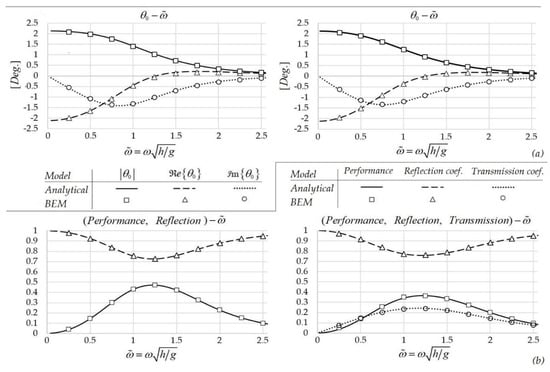
Figure 2.
Comparison between Boundary Element Method (BEM) numerical results (shown using symbols) and analytical solution (shown using lines) for terminator-type OWSC: (a) the special case of absorbing–reflecting model (left column subplots) and (b) the standard absorbing–radiating model (right column subplots). (a) Angular response and (b) performance, for incident wave height H = 1m and water depth , and the following set of parameters: .
2.4. Performance of OWSC in Variable Bathymetry
In this section, we present results concerning the calculation of device performance in regions of non-uniform bathymetry, characterized by a depth function h(x). For comparison purposes, all other parameters of the studied 2dOWSC remain the same as in the example previously presented in Figure 2. We first consider a shoaling environment as presented in the top subplots of Figure 3. The variable bathymetry subdomain is defined between two subregions of constant but different depth: the region of wave incidence with depth 25 m, and the vicinity of the device with depth 10 m, that remains constant in the downwave region, behind the flap. The water depth in the upwave subregion is defined by the function:
which describes a smooth shoal with maximum bottom slope controlled by the parameter , while is a function of finite support, modelling additional bottom corrugations. The parameter denotes the position of the maximum bottom slope, selected here to coincide with the middle x-coordinate of the domain. The seabed profiles shown in the upper left and right subplots of Figure 3 are determined, for , by setting the parameters as and , respectively.
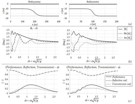
Figure 3.
Performance of the examined system in variable bathymetry corresponding to smooth underwater shoals. (a) Depth profiles, (b) Oscillation angle charts, (c) Performance, Reflection and Transmission coefficients as functions of the nondimensional frequency. Incident wave height H = 1 m and water depth in the far upwave region . .
In particular, in Figure 3b the calculated real and the imaginary part of the complex amplitude , as well as its absolute value, are plotted as a function of the non-dimensional frequency, while the graphs in Figure 3c depict the performance of the device and the reflection coefficient (R) and transmission coefficient (T) as functions of the same parameter. The water depth at the device’s boundary is used for nondimensionalization.
A maximum value of performance about 39% is observed for nondimensional frequency . According to the results shown in the above graphs, the maximum angle achieved during the oscillation is not substantially affected by changes in bathymetry (see Figure 2). On the other hand, the angular responses, especially in the low frequencies, differ significantly compared to the corresponding predictions at constant water depth, due to strong the interaction of the incident waves with the seabed. The observed oscillations in the numerical results are due to variations in the phase of various quantities excited by depth irregularities. By comparing the results presented in Figure 3 to the ones presented in the right column of Figure 2, we observe that as the mean bottom slope reduces, the responses and the performance converge to the results obtained at constant depth. On the other hand, as the bottom slope increases, there is a strong effect on the flap’s oscillation phase, particularly at lower frequencies, due to stronger wave–seabed interaction.
On the contrary, abrupt changes occurring over a short horizontal distance less affect the flap’s oscillation phase, but have a stronger effect on the performance curve, in the bandwidth of frequencies in which there is interaction of the incident waves with the seabed. Βy using an auxiliary grid spanning the entire two-dimensional domain, the distribution of the velocity potential can be calculated by the superposition of the potential induced from each one of the boundary elements to each point of the auxiliary grid. After obtaining the values of the complex wave potential on every point of the 2D grid, the induced field can be represented at any moment (t) by the real part of φ multiplied by . Figure 4 illustrates the wave field during the OWSC’s operation in a non-uniform bathymetry region, whose seabed profile is defined by Equation (20) for , by means of equipotential lines. For the specific period of 8 s (), the resulting reflection coefficient is R = 0.8287, and thus the performance of the device equals P = 31.32%. It can be observed that the wave field resembles an almost stationary wave for fractions of the period, and propagates gradually depending on the flap’s oscillation phase. Furthermore, it can be seen that the wave potential’s field satisfies the Neumann boundary condition Equation (14) on the seabed boundary, which is equivalent to the fact that the equipotential lines intersect the impermeable bottom perpendicularly.
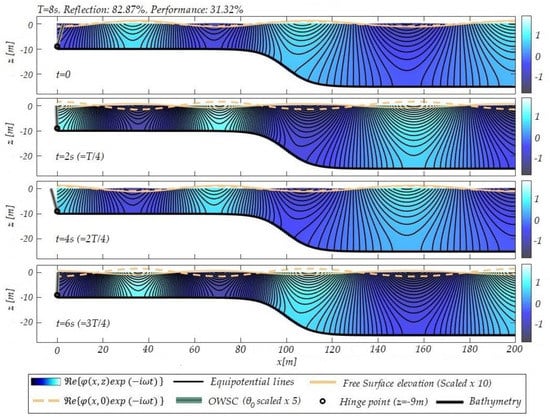
Figure 4.
Equipotential lines of the wave field and free surface elevation at different times as calculated by the present BEM in the case of the absorbing–reflecting model in a shoaling topography .
Apart from seabed profiles characterized by depth changes described by hyperbolic tangent functions, the present BEM is applicable to more realistic bathymetric variations which can be determined by considering bottom corrugations (in addition to shoaling effects). Such inhomogeneities can be determined by, among other ways, adding a damped sine or cosine term to the function describing the seabed. Before applying the method, one must ensure that the parameter selection leads the additional term completely dying out, in both the areas of the two vertical boundaries. As an example, we consider in Figure 5a the depth profile [Equation (20)], with and bottom corrugations For comparison purposes, all other parameters remain unchanged. The plot in Figure 5b illustrates the real and the imaginary part of the complex amplitude, as well as its absolute value, as a function of the nondimensional frequency, while Figure 5c of the figure depicts the performance of the device, and the reflection (R) and transmission (T) coefficients, as a function of the same parameter. The water depth at the device’s boundary is used for nondimensionalization. Ιn relation to the corresponding graphs of Figure 3, it can be observed that the current alteration of the seabed profile introduces a significant difference to the device’s performance in the bandwidth of the nondimensional frequency between 0.5 and 1. The wavelengths falling into this bandwidth are 60 m to 170 m long, and thus result in strong interaction with the seabed.
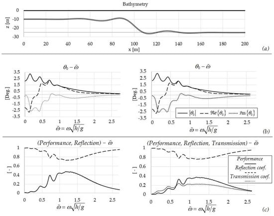
Figure 5.
Performance of studied system in variable bathymetry corresponding to underwater shoal in conjunction with bottom corrugations: (a) the special case of absorbing–reflecting model (left column subplots) and (b) the standard absorbing–radiating model (right column subplots). (a) Depth profile, (b) Oscillation angle chart, (c) Performance, Reflection and Transmission coefficients as a function of the nondimensional frequency. .
Figure 6 illustrates the calculated wave field during the absorbing–reflecting termination type OWSC operation in the non-uniform bathymetry region, whose seabed profile is defined by Equation (20) for the aforementioned parameter selection, by means of equipotential lines. For the specific period of 8 s, the resulting reflection coefficient is R = 0.8455, and thus the performance of the device equals P = 28.50%. The excellent satisfaction of the bottom boundary condition in the examined irregular seabed topography is clearly observed.
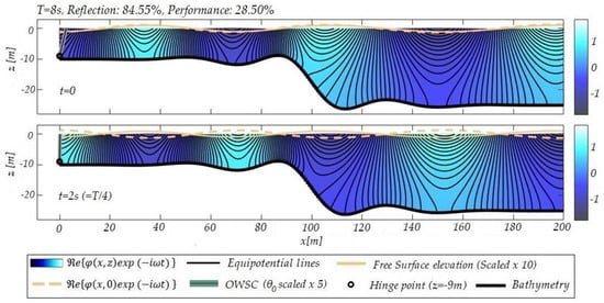
Figure 6.
Equipotential lines of the wave field and free surface elevation at different times as calculated by the present BEM in the case of the absorbing–reflecting model in a variable bathymetry region .
3. WEC Model
In this section, the BEM model developed by the authors of [8,9] is briefly reviewed. This model will be used to obtain numerical results concerning the performance of point absorbers, and present comparative results concerning an application to a nearshore/coastal site in Greece that will be presented in the next section. The point absorber is modelled by an axisymmetric floating body with radius a and draft T, operating in a coastal environment. As before, the bathymetry corresponds to the shoaling seabed profile with depth smoothly ranging from in the region of incidence, to in the region of transmission. As excitation of the floating device is assumed a harmonic wave of angular frequency ω and incident direction. For a relatively small wave slope, remaining within the limits of the linear theory, the wave potential and free surface elevation are:
where denotes the horizontal coordinates and is the frequency parameter. The wave potential is decomposed on the propagating wave potential , with the absence of the floating body, the diffraction potential due to the presence of the impermeable and motionless geometry of the WEC and the radiation potential , which is the summation of the radiating fields due to the six modes of oscillation of the WEC:
On the wetted surface of the WEC, the following boundary conditions are applied:
where is the normal vector directing inwards the geometry of the floater, and is the component of the normal vector in generalized form. Considering that heaving is the only power mode of the WEC, its response in the vertical oscillation can be obtained as:
In the above expression of heave response amplitude operator-ξ3 (RAO ξ3), the implemented Froude–Krylov Xp and diffraction XD exciting forces are evaluated by integration of the wetted surface of the body , as follows:
while is calculated by:
The hydrodynamic coefficients of added mass (α33) and damping (b33) in Equation (26) are obtained by integrating the heave-radiation potential on the submerged boundary surface of the WEC:
In addition, = ρgAWL is used for the hydrostatic coefficient and AWL refers to the waterline surface. Finally, Bs and Cs are the damping and spring coefficients of the involving linear PTO system, respectively. The expression for the time-averaged WEC power output of a WEC in heave power mode follows:
where is the PTO efficiency. The amount of the available wave power that can be harnessed by the device depends on the directional wave spectrum and PTO characteristics; see [8,9].
Evaluation of Wave Field
The total wave field, as already described, can be decomposed into mainly three quantities: the propagation field, the diffracted field and the radiated field. The Coupled Mode Model, developed in [12] and extended to 3D in [13], is used for the evaluation of the propagation field, over bathymetric topographies with even steep depth steps, where analytic solutions are infeasible, ensuring the energy conservation at the same time. The main formula is based on the following local-mode representation, with the enhancement of correction terms in order to globally satisfy the boundary condition of the rigid bottom:
The vertical functions Zn (z; x) are obtained as eigenfunctions of regular Sturm–Liouville problems, formulated at the local depth, while the functions are the complex amplitude of the nth-mode, and are found as the solution of the following Coupled Mode System (CMS)
where the coefficients , defined in terms of the vertical eigenfunctions, are described in Table 1 of Reference [13]. The CMS is also supplemented with boundary conditions to treat incidence, reflection and transmission phenomena over regions of general bathymetry.
For the evaluation of the diffraction and radiation potentials, a BEM method, developed in [14] and described in [8,9], is used. More specifically, the induced potential and velocity from the 4-node quadrilateral elements, used for the discretization of all the boundaries (body, free surface and seabed surface), is expressed as:
where summation refers to all the quadrilateral elements, and Φp and Up are used to denote, respectively, the potential and velocity induced from the pth element of unit singularity distribution to a random field point . These quantities, induced from each element, can be evaluated by semi-analytical expressions, and the final discrete solution is obtained using the collocation method, aiming to satisfy the boundary conditions at each panel’s centroid.
The aforementioned BEM, used to treat the hydrodynamic problem of a point absorber-type WEC, even in cases of operation over arbitrary bathymetric regions, is developed, validated against analytical solutions whenever possible, and used to obtain useful information regarding the response and power output of the devices, and assist the research towards optimized WECs and efficiency maximization, assuming cases of one-device installation or array deployments; see [8,9].
4. Application to A Specific Coastal Site in Greece
Greece is located at the eastern Mediterranean Basin, and its energy sector is still largely dependent on fossil fuels (coal and oil). On the other hand, the coastline extents to 16,000 km, and therefore marine renewable energy could be a contributor to the power production, especially as concerns the supply of islands. The Aegean Sea region is characterized by high wind potential, which gives rise to relatively intense wave activity. However, the wind fetches are not very long, due to the presence of island complexes. Nonetheless, channeling effects cause certain spots to develop high wave potential [15,16].
Estimation of the mean annual wave power in the Greek Sea region has been presented by various authors, based on calibrated hindcast wave data (e.g., see [15,16]). A nearshore hot spot which is exposed to relatively long wind fetches, corresponding to increased wave potential, is located at the nearshore area of the south-eastern part of Evia Island, in the central Aegean Sea. This region is highlighted in Figure 7.
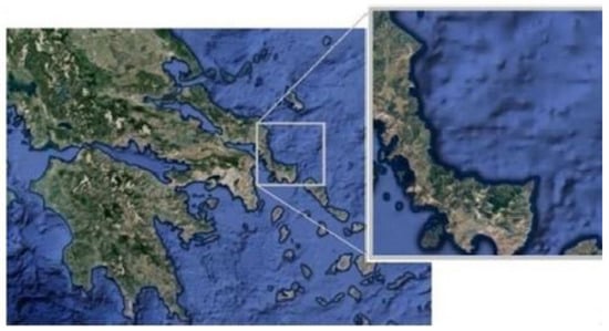
Figure 7.
Nearshore area of south-eastern part of Evia Island, in the central Aegean Sea (Source: Google Maps).
Wave energy devices are usually located relatively close to the shoreline. Hence, the vast majority of wave energy applications rely on the prediction of wave power availability in nearshore areas. Nonetheless, the data provided by global forecasting models, satellite or buoy measurements are available for off-shore regions. In order to obtain the near-shore wave conditions, the transformation of offshore sea states is required. This is achieved by using wave models for the transformation of waves using offshore wind and wave data, in conjunction with geographical (bathymetric and coastline) information in the examined area (e.g., see [17,18]). The geographical area considered in this study is enclosed by the box [24°10′E, 24°40′E]–[38°05′N, 38°30′N]. The area is shown in the map of Figure 8a, along with the nearest offshore data points (O1, O2 and O3). In a previous work [18], five representative nearshore target points of the specific area were studied in order to transform the offshore sea states and obtain the nearshore wave potential. The detailed analysis showed that the nearshore area around TP5 (North side of Cape Kafireas) is where the available wave potential is maximized. This site is furthermore suitable for the installation of a wave energy park, since it is not very close to villages, and there is the possibility of grid connection. The target points (TP) are shown in Figure 8a using circles. A nautical map illustrating the seabed’s morphology in the area, by means of isobath lines, is presented in Figure 8b.
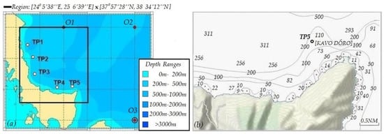
Figure 8.
(a) Map of the south-eastern part of Evia Island. Domain of wave calculation, offshore data points (Oi) and nearshore target points (TPi). (b) Nautical map of the region around the point TP5.
The wave data used in the study are available from the EUROWAVES database, in the form of time-series covering the 8-year period of 1992–1999, regularly sampled at 6-hour intervals, with a total sample size of 10,189 [18]. The overall mean value of the available wave potential in the offshore area (point O2) is equal to 7.2 kW/m. The calculated nearshore wave climatology is presented in Figure 9, and details concerning the analytical probability models used for univariate and multivariate data can be found in [19,20]. Based on the nearshore wave data, the annual distribution of the wave potential for the point TP5 is shown in Figure 10a, and the mean value is dropped to 3.86 kW/m. The mean monthly distribution is also presented in Figure 10b. The maximum value of available wave power (≈6 kW/m) is observed in winter, while it becomes lowest during spring (≈2 kW/m).
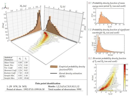
Figure 9.
Annual distribution of wave parameters at the nearshore point TP5.
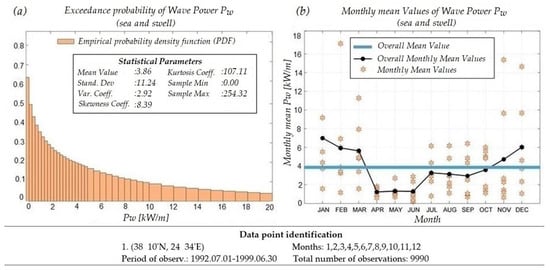
Figure 10.
Annual distribution of wave potential at the nearshore point TP5.
4.1. Estimation of Power Output by Application of OWSC
We next consider an OWSC device positioned along the 20-m isobath in the examined nearshore/coastal area. Due to the fact that the seabed slope in the nearshore area is very mild, we consider as a first approximation that the wave conditions at the OWSC (depth 20 m) remain the same as in TP5 (depth 137 m). Thus, for each pair of mean energy period and significant wave height of the nearshore climatology (Figure 9), the captured wave power per meter of wavefront is calculated by multiplying the resulting wave power flux per meter by the value of the device’s performance curve that corresponds to the given period.
Although the present model is restricted to two dimensions, it is approximately used in this section to investigate the effects of the geometrical inhomogeneities of the seabed boundary on the performance of the considered devices. The results concerning power output estimations are considered preliminary, and will be updated by future extensions of the present model to treat realistic three-dimensional and real fluid effects.
Using the analytical model described in the Appendix A, the PTO parameters are first optimized, and at a next step the shoaling effects on the OWSC performance are calculated by means of the present BEM model. The results are obtained under the assumption of a very narrow spectrum, and are based on summing monochromatic components. The device axis of rotation is positioned at a distance of 1 m above the seabed (d/h = 19/20). The site-specific Performance Index (P.I.) of the OWSC is defined as the percentage of the energy captured over the wave power contained in the whole data set, which is calculated by
where N is the sample size of the wave climate data at TP5. Figure 11 illustrates the site-specific Performance Indices, as calculated for various combinations of the PTO parameters, as well as the flap material density (defined relatively to the sea water density). Each point of the graphs corresponds to the Performance Index [Equation (33)] of an OWSC positioned at 20 m depth, for the given parameters, as calculated by the analytical model.
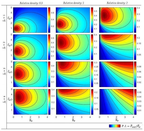
Figure 11.
Site Specific Performance Indices (Based on the analytical model for h = 20 m, d/h = 19/20).
In the sequel, in order to present more specific results, we shall restrict the analysis to an OWSC flap of relative density equal to 0.5, and with a nondimensional inertia parameter equal to . Figure 12 illustrates the site-specific performance indices along with resulting performance curves, presented as functions of the non-dimensional frequency. First, it is noted that the value of the nondimensional frequency which corresponds to the most probable period of the incident waves in the area, as obtained from the nearshore/coastal climatology (T ≈ 3.5 s), is equal to:
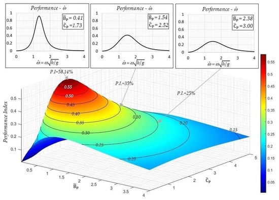
Figure 12.
Site-specific Performance Index of the Oscillating Wave Surge Converters (OWSC) equipped with a Power Take Off (PTO) system characterized by the corresponding parameters, along with specific resulting performance curves. (Based on the analytical model, using ).
Interestingly, we observe in Figure 12 that the optimal (maximum) Performance Index (= 58.14%) does not occur for configurations with eigenperiod coinciding with the above value of the mean period for the incident waves, but for OWSC configurations whose peak performances are achieved for greater oscillation periods of around 6.2 s, which is significantly higher. An explanation for this fact is that, although waves characterized by periods of about T = 3.5 s–4 s occur relatively often due to the climate characteristics of the considered region, these waves are associated with relatively low wave heights, and their energy contents are lower. On the other hand, the occurrence of waves characterized by a reasonably increased value of period of (e.g., Τ > 10 s) is very scarce in the specific geographical area.
A normalized distribution of the available wave energy, with respect to the incident period associated with the population of waves in the nearshore/coastal area examined, is presented in Figure 13, as obtained from the climatological data of Figure 9. It is clearly seen in this figure that the wave period with the largest energy content for the specific region’s wave climate characteristics is around 6.2 s. The latter result provides useful information concerning the selection of the PTO parameters of the device for the maximization of power capture in the specific area. In particular, the value of the corresponding nondimensional frequency is equal to , justifying the selection of a flap of relative density equal to 0.5 and PTO system parameters , which results in a performance curve with a peak of 40%, for a frequency close to the optimal operating point. The latter values will be used in the next part of the present study in order to investigate the effects of variable seabed topography by means of the developed BEM scheme.
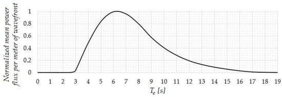
Figure 13.
Distribution of available wave energy at TP5 as a function of the incident wave period.
4.2. Bottom Topography Effects
As stated earlier, the water depth at the point TP5 is equal to 137 m. Furthermore, as shown in Figure 8b, the distance between point TP5 and the shoreline is approximately equal to 1 NM (≈1850 m). Assuming that the OWSCs array is located 150 m from the shoreline, the upwave length of the domain is 1700 m, and the seabed profile is modelled using Equation (20), as follows:
As previously discussed, relatively mild bottom slopes do not significantly affect the performance of the device. Applying the BEM, in the above domain and for the specific PTO parameters, results in the performance curve shown in Figure 14a,b. The corresponding results obtained by the analytical model, for a constant depth of 20 m, are presented in Figure 14c,d.
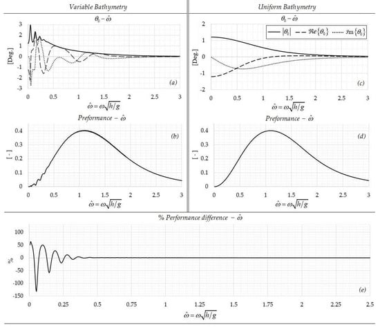
Figure 14.
Oscillation angle (a,c) and Performance (b,d) charts as a function of the nondimensional frequency, for variable and uniform bathymetry. (e) Percentage difference between the two performance curves .
The Performance Index, which results from calculating the percentage of the power that is captured for the given performance curve, was found to be equal to 34.6%, and differs by a small amount from the result at a constant depth (which is 34.8%). This implies that the effects of the seabed’s profile in this case are negligible. As depicted in Figure 14e, significant alterations to the performance curve, due to bathymetry inhomogeneities, occur within the bandwidth of the nondimensional frequency between 0 and 0.5, which corresponds to incident wave periods of 18 s or more. This corresponds to long swells, which result in strong seabed–wave–device interaction. Such data, however, are not present in the climatology of the specific coastal area, and thus, the variable bathymetry causes negligible changes in the performance of the OWSC. Nonetheless, in other cases possibly characterized by different wave statistics and stronger seabed topography variations, the sloping bottom effects are expected to be significant, and can be fully accounted for by the present model.
Based on the above calculated performance of the OWSC, the monthly mean power output, per meter of wavefront, in the examined nearshore/coastal area is presented in Figure 15a. Moreover, the monthly mean percentages of power capture are depicted in Figure 15b. It can be observed that the device’s performance is slightly reduced during the spring season, and appears increased during the winter months. This is mainly due to the variability of the monthly mean incident wave period, which results in a shifting of the device’s operation point on the performance curve, and leads to different fractions of the incident wave energy being captured. Subsequently, we assume an array of three OWSCs positioned along the 20-m isobath in the coastal area, and over the 20-m isodepth in the nearshore area, of the TP5 point, as shown in Figure 16. Each OWSC is considered to be 20 m wide. The assumed device’s spacing is defined in order to ignore, as a first approximation, interaction effects. Furthermore, the device’s width could modify the system’s eigenperiod, and such effects are left to be examined in future work extending the present method to 3D applications.
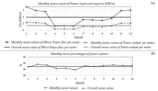
Figure 15.
(a) Monthly mean values of power input and output in kW/m; (b) Monthly mean percentages of power capture .
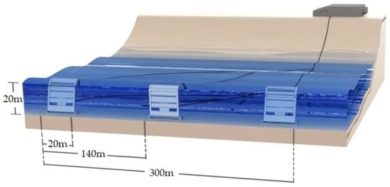
Figure 16.
Considered OWSC array.
The considered OWSC array is illustrated in Figure 16. Given that the results were extracted via a two-dimensional analogue, which refers to unit length in the third dimension, the power output of any unit of the considered OWSC park can be estimated by multiplying the power output per meter of wavefront with the unit’s width. An average of 5% losses was assumed due to the unit’s shut down for maintenance or repair works after failure (ηop = 0.95), and 2% losses due to transmission efficiency (ηtr = 0.98; see [21]). The monthly mean power output values of the OWSC energy park can then be obtained by multiplying the unit’s output power with the number of OWSCs, and the result concerning the estimated corresponding monthly mean power output in [kW] is depicted in Figure 17.
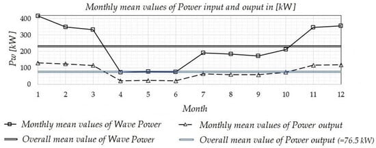
Figure 17.
Monthly mean values of power input and output in kW .
Eventually, the annual energy production (AEP) of the OWSC array is approximately estimated (in kWh) by multiplying the annual averaged electrical power output of the park by the total number of operating hours within a year, as follows:
4.3. Estimation of Power Output by Point Absorbers and Comparative Evaluation
For comparison purposes, the installation of an energy park, consisting of an array of point absorbers, is examined here, using the model presented in a previous section. The park is located in the exact same geographic area. The array consists of six point absorber buoys, with a diameter of 10 m, so that the total distance covered by wave energy-exploiting devices remains unchanged relative to the previously examined park (60 m), as illustrated in Figure 18. For the purposes of the comparative analysis, an indicative performance curve of these devices was adapted from [8,9].
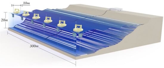
Figure 18.
Considered array of point absorbers.
The performance curve of the WEC point absorber is based on the assumption of a typical PTO damping coefficient, with an indicative value considered as 10 times the mean value of hydrodynamic damping coefficient . The expression used in [8,9] for the nondimensionalization of the incident waves’ frequency involves the heaving cylinder’s radius. Therefore, based on the considered diameter, the performance of the buoys can be expressed as a function of the nondimensional frequency , as depicted in Figure 19.
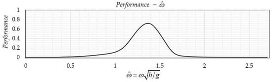
Figure 19.
Performance of heaving buoys as a function of the non-dimensional frequency .
It can be observed in Figure 19 that the maximum performance achieved is about 70%, for , which implies a natural period of around 6.5 s, compatible with the peak of the distribution of available wave energy at TP5. The monthly mean power output per meter of wavefront, based on the nearshore data calculated for the wave climate in TP5 (Figure 10) and the WEC performance curve of Figure 19, is presented in Figure 20a. Moreover, the monthly mean percentages of power capture are depicted in Figure 20b. It can be observed that the device’s performance differs significantly between months, which is a result of the increased performance in a very limited frequency range, which mainly occurs during winter, based on the available wave climate data.
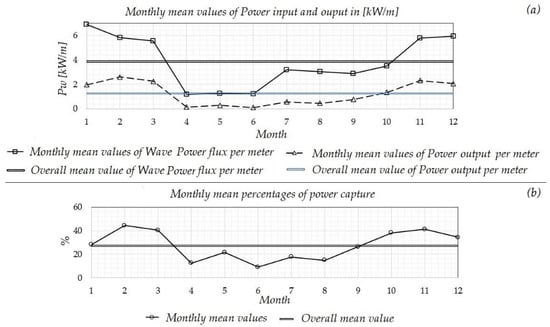
Figure 20.
(a) Monthly mean values of power input and output in kW/m (b) Monthly mean percentages of power capture .
The power output of any unit of the considered point WEC array can be estimated by multiplying the power output per meter of wavefront with the unit’s diameter. The losses due to device availability and transmission efficiency are considered to be the same as before (ηop = 0.95, ηtr = 0.98). Therefore, for the WEC array of Figure 18, the estimated corresponding monthly mean power output is the one depicted in Figure 21. The annual energy production (AEP) is 0.581 GW/h. The AEP of the point absorbers array is found to be lower than that of the OWSCs park by a factor of around 15%, despite the fact that the performance curve of the heaving buoys reaches a maximum value of 70%, which is greater than that of the OWSC. This is due to the limited frequency range within which the considered WEC performance (without fancy control) is increased, in comparison to the OWSC response and performance, which is more broadband.
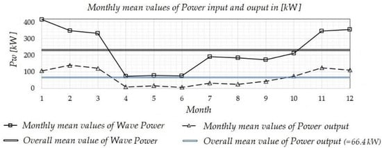
Figure 21.
Monthly mean values of power input and output in kW .
Specifically, unlike OWSCs, which are excited by the wave field in a significant fraction of the fluid channel, the point absorber buoys only exploit the power flux concentrated near the free surface’s level. As a result, the performance indices corresponding to frequencies that imply shallow water wave propagation are relatively lower for this type of energy device.
The above analysis is based on a simplified extension of a two-dimensional analogue, and therefore all the effects induced from the three-dimensional nature of the phenomenon, as well as oblique wave incidence, are neglected. The function of individual point absorbers is independent of the propagation direction of the excitation wave field. However, this is not the case for arrays or grids consisting of several such devices, due to the hydrodynamic interactions between the different units. The latter effects are left to be examined in more detail in future works.
In conclusion, the proper design and dimensioning of the wave energy technologies, as the ones studied here, can lead to significant exploitation of marine renewable energy. In addition, with appropriate optimization of device parameters, taking into account the wave climatology of the considered location of installation, significant output can be achieved. As regards Greece’s nearshore/coastal region, the development of wave energy parks would probably lead to increased energy costs, except for sites with increased wave potential. However, as the relative technology and know-how reach new levels of maturity, the costs associated with designing and manufacturing wave energy devices will most likely reduce, and from this perspective, the development of wave energy parks in Greece is likely to take place in the near future. For this purpose, more detailed investigation of various successful devices and concepts is needed in order to identify the most efficient solution.
5. Conclusions
In this work a simplified BEM is developed and applied to the investigation of variable bathymetry effects on the performance of surge-type wave energy converters (OWSC) excited by harmonic incident waves. The terminator-type model is studied in two dimensions, where the flap of the device is aligned perpendicularly to the incident wave direction. On top of the standard absorbing–radiating model, which includes additional effects due to wave transmission in the downwave region behind the flap-board, the special case of absorbing–reflecting model is also considered. Although the present study is restricted for simplicity to two dimensions, the model offers a useful tool that could be systematically applied, with low computational cost, to investigate the effects of the geometrical inhomogeneities of the seabed’s boundary, and could support future extensions into more realistic three-dimensional configurations.
The present method is first validated with the prediction of results against analytical solutions derived at a constant depth. Subsequently, the relation between the various sea states and the device performance is investigated by systematic application of the BEM model, and the effects of several important parameters that characterize the configuration are examined and discussed. Numerical results, illustrating the modification of the wave field and the effects of depth variation in conjunction with other parameters, like inertia and power-take-off, are illustrated.
It is also shown that the effects of bottom slope and curvature, especially on the response and secondly on the performance of the studied device, could be important, especially for low and moderate wave frequencies, and should be taken into account. Finally, the installation of wave energy devices in specific nearshore/coastal regions of Greece, characterized by increased potential, is examined, and the power output from OWSCs is compared with WEC point absorber installations. Future work will be directed towards the extension of the present model into studying the responses and the performance of three-dimensional systems in more realistic, irregular and general-incidence wave conditions, as well as the consideration of non-linear effects.
Author Contributions
Conceptualization, K.B.; methodology, K.B., A.M. and M.B.; software, A.M. and M.B.; validation, A.M. and M.B.; formal analysis, A.M. and M.B., writing—original draft preparation, A.M. and M.B.; writing—review and editing, K.B., supervision, K.B. All authors have read and agreed to the published version of the manuscript.
Funding
This research received no external funding.
Conflicts of Interest
The authors declare no conflict of interest.
Abbreviations
| BEM | Boundary Element Method |
| CMS | Coupled Mode System |
| OWSC | Oscillating Wave Surge Converter |
| PTO | Power Take Off |
| TP | Target Point |
| WEC | Wave Energy Converter |
Appendix A. Linearized 2dOWSC Model in Constant Water Depth
Assuming, for simplicity, the two-dimensional problem concerning normally incident waves at a constant depth, the linearized model of the considered terminator flap-type model is shown in Figure A1. In particular, except of the standard absorbing–radiating model depicted in Figure A1a, which includes additional effects due to wave transmission in the downwave region behind the flap-board, an absorbing–reflecting model, shown in Figure A1b, is also considered. Although the latter configuration could be represented by appropriately adjusting the PTO parameters to achieve zero transmitted wave, it is still considered here as a special configuration of the 2dOWSC problem, and the solution is used for the validation of the developed BEM.

Figure A1.
Simplified 2D model of terminator-type OWSC in constant water depth: (a) the standard absorbing–radiating model, and (b) the special case of an absorbing–reflecting model.
Given that the flap motion is generated by incident waves, a fraction of the incoming wave energy (I) received by the device is expected to be reflected (R), while in the case of the more general absorbing–radiating model, another fraction is transmitted (T). Considering that the flap performs harmonic angular oscillations, of maximum width θ0 with frequency ω, the angle of oscillation at any time is given by:
In order to ensure that the system will perform harmonic oscillations, a torsional spring at the hinge point is considered, which restores the flap after its deviation from the vertical position during each period, due to the incident waves. Moreover, the hydraulic generator, which compresses fluid and supplies the hydroelectric power station, uses part of the oscillation’s energy, and therefore acts as a damper in the contemplated torsional oscillator. For simplicity, power extracted by the system (PTO) is considered to be converted into electricity at the hydroelectric power station, without any further losses, e.g., due to transmission through the pipeline system, or mechanical losses. The equation for the motion of the angular oscillator is:
where is the moment of inertia of the flap with respect to the axis of rotation, is the damping coefficient associated with the PTO, is the spring constant of the installed torsional spring and M(t) is the time dependent torque that the flap receives from the waves. Assuming small angles of deviation from the vertical position (), the horizontal velocity of any point on the flap will be equal to:
and indicates the lever arm of a given point on the flap, located at depth , with respect to the center of rotation, and is the hinge point’s depth; see Figure A1. Given the assumption of small angles of deviation from the vertical position (), the horizontal excursion of the flap motion at the free surface level is:
The general expression of the complex potential describing the wave field in the semi-infinite constant depth strip is as follows:
where and H is the incident wave height. The first term in Equation (A5) corresponds to the left-propagating mode. R represents the complex amplitude of the reflected component and represent the corresponding amplitudes of the evanescent modes. In the case of the more general absorbing–radiating model of Figure A1a, the expression of the wave potential in the downwave region behind the flap-board is given by:
where T represents the complex amplitude of the transmitted wave and are the corresponding evanescent modes. Moreover, represents the vertical structure of each mode, while and are obtained as the real and imaginary roots of the dispersion relation:
The free surface’s elevation is given by:
By using the above representations, the free surface elevation in the upwave direction can be expressed as:
and in the case of the more general absorbing–radiating model of Figure A1b, the free surface elevation in the downwave direction is:
The boundary condition on the surface of the flap specifies that the horizontal body velocity is equal to the fluid’s horizontal velocity for , and in terms of the complex potential φ, it is expressed as follows:
The above boundary condition must be satisfied by the wave potential, along with the free surface and bottom boundary conditions, which respectively are:
The x-derivative of the wave potential provides the horizontal component of the fluid’s particles’ velocity in the flow field. The latter evaluated at the position of the flap x = 0 reads as follows:
In the case of the more general absorbing–radiating model of Figure A1a, the x-derivative of the wave potential in the downwave side is obtained from Equation (A5b) as
By expressing the function f(z) of the horizontal velocity of the flap in terms of the vertical eigenfunctions , and using it in the boundary condition Equations (A9) and (A11), we obtain the following relations for the coefficients , and , Bn, respectively:
where
The equation of motion of the angular oscillator [Equation (A2)] is expressed in the frequency domain as follows:
where is the moment applied to the flap as a result of the fluid’s pressure from the upwave side, and is the moment due to pressure forces from the downwave side, which is only included in the open-type model. The latter quantities are expressed in terms of the complex wave potential by integrating the pressure forces evaluated from a linearized Bernoulli’s equation , multiplied by the lever arm across the flap’s length:
which respectively become
Using Equation (A12) and substituting in the above the coefficients R and An, and T and Bn, respectively, we finally get:
and
By using the above in Equation (A14) and solving for , we obtain for the angular response of the system:
where
and the coefficient
in the absorbing–reflecting model, while B = 1 for the absorbing–radiating model. Finally, by substituting the flap angular response (θ0) in the Equations (A12), the coefficients R and An, and T and Bn, are calculated. The complex wave potential and the free surface elevation are obtained from Equations (A5) and (A8), respectively.
The performance of the device is estimated as the fraction of the power input that is converted into beneficial output power. The average wave power (Pin) associated with the incident wave is given by:
where is the group velocity of water waves in the constant depth strip:
The average output power converted by the device is calculated through the damping coefficient (modelling the hydraulic generator) as:
Subsequently, the Performance Index () of the device can be estimated by the quotient of the two above. In addition, for a given incident wave height H, the reflected wave height will be equal to
, and in the case of the open-type model (B = 1), the transmission coefficient is equal to , and thus,
is a relation that can be used to verify conservation of energy in the examined hydromechanical system.
In order to illustrate the numerical performance of the above simple model, the following dimensionless parameters are introduced concerning the coefficients of the OWSC Power Take Off model:
where ρm represents the density of the flap’s material. It is noted that, since a two-dimensional analogue of the flap type surge converter is being considered, all the terms of the differential equation of motion of the angular oscillator refer to their respective units per unit length in the transverse direction. The extension of the model for the study of three-dimensional phenomena will be examined in future work.
As an example, we consider an OWSC, with non-dimensional PTO parameters equal to and density ratio ρm/ρ = 1, operating in water depth equal to h = 10 m, with the device’s hinge point located at the depth of 8 m (d/h = 0.8). Numerical results are presented in Figure A2 for incident waveheight H = 1 m, illustrating the calculated performance of the examined system obtained by keeping 10 terms in the modal series Equation (A5), which is found to be enough for the convergence of the results in the whole band of frequencies considered. Both absorbing–radiating and absorbing–reflecting systems have been considered, and the results concerning the angular response and the reflection–transmission characteristics are plotted in the upper and lower subplots of Figure A2, respectively.

Figure A2.
(a) Oscillation Angle Chart, (b) Performance, reflection and transmission coefficients, as a function of the nondimensional frequency in the case of terminator-type OWSC at a constant depth: the special case of absorbing–reflecting model (left column subplots), and (b) the standard absorbing–radiating model (right column subplots). (a) Angular response and (b) performance, for incident wave height H = 1 m and water depth H = 10 m, and the following set of parameters: .
More specifically, the first-row subplots of Figure A2 illustrates the real and the imaginary part of the calculated complex amplitude θ0, as well as its absolute value, as a function of the nondimensional frequency. Moreover, the second-row subplots depict the performance of the studied device (plotted by using thick solid lines) and the reflection coefficient R (plotted by using dashed lines), while in the case of the open-type system the transmission coefficient is also included (by using dotted lines). It is worth noticing that the conservation of energy expressed by Equation (A23) is perfectly satisfied for both examined types and for all frequencies. We also observe in this figure that in the case of the more general absorbing–radiating system, the calculated performance is a few percent lower than in the absorbing–reflecting system, due to additional losses associated with radiating wave energy in the downwave side of the flap-board. On the other hand, the change concerning the angular response of the flap is much smaller.
References
- Falnes, J. Ocean Waves and Oscillating Systems, 1st ed.; Cambridge University Press: Cambridge, UK, 2002. [Google Scholar]
- Babarit, A. Ocean Wave Energy Conversion, 1st ed.; ISTE Press-Elsevier: Amsterdam, The Netherlands, 2017. [Google Scholar]
- Whittaker, T.; Folley, M. Nearshore oscillating wave surge converters and the development of Oyster. Philos. Trans. R. Soc. 2012, 370, 345–364. [Google Scholar] [CrossRef]
- Renzi, E.; Doherty, K.; Henry, A.; Dias, F. How does Oyster work? The simple interpretation of Oyster mathematics. Eur. J. Mech.-B/Fluids 2014, 47, 124–131. [Google Scholar] [CrossRef]
- Whittaker, T.; Folley, M.; Osterried, M. The oscillating wave surge converter. In Proceedings of the International Society of Offshore and Polar Engineers (ISOPE), Toulon, France, 23–28 May 2004. [Google Scholar]
- Dias, F.; Renzi, E.; Gallagher, S.; Sarkar, D.; Wei, Y.; Abadie, T.; Cummins, C.; Rafiee, A. Analytical and computational modelling for wave energy systems: The example of oscillating wave surge converters. Acta Mech. Sin. 2017, 33, 647–662. [Google Scholar] [CrossRef] [PubMed]
- Folley, M.; Whittaker, T.; Henry, A. The effect of water depth on the performance of a small surging wave energy converter. Ocean Eng. 2007, 34, 1265–1274. [Google Scholar] [CrossRef]
- Belibassakis, K.A.; Bonovas, M.; Rusu, E. A novel method for estimating wave energy converter performance in variable bathymetry regions and applications. Energies 2018, 11, 2092. [Google Scholar] [CrossRef]
- Bonovas, M.; Belibassakis, K.A.; Rusu, E. Multi-DOF WEC performance in variable bathymetry regions using a hybrid 3D BEM and optimization. Energies 2019, 12, 2108. [Google Scholar] [CrossRef]
- Babarit, A.; Hals, J.; Muliawan, M.; Kurniawan, A.; Moan, T.; Krokstad, J. Numerical benchmarking study of a selection of wave energy converters. Renew. Energy 2012, 41, 44–63. [Google Scholar] [CrossRef]
- Katz, J.; Plotkin, A. Low-Speed Aerodynamics, 2nd ed.; Cambridge University Press: Cambridge, UK, 2001. [Google Scholar]
- Athanassoulis, G.A.; Belibassakis, K.A. A consistent coupled-mode theory for the propagation of small-amplitude water waves over variable bathymetry regions. J. Fluid Mech. 1999, 389, 275–301. [Google Scholar] [CrossRef]
- Belibassakis, K.A.; Athanassoulis, G.; Gerostathis, T. A coupled-mode model for the refraction–diffraction of linear waves over steep three-dimensional bathymetry. Appl. Ocean Res. 2001, 23, 319–336. [Google Scholar] [CrossRef]
- Belibassakis, K.A.; Gerostathis, T.; Athanassoulis, G.; Soares, C. A 3D-BEM coupled-mode method for WEC arrays in variable bathymetry. In Proceedings of the 2nd International Conference on Renewable Energies Offshore (RENEW2016), Lisbon, Portugal, 24–26 October 2016. [Google Scholar]
- Soukissian, T.; Gizari, N.; Chatzinaki, M. Wave potential of the Greek seas. WIT Trans. Ecol. Environ. 2011, 143, 203–213. [Google Scholar] [CrossRef]
- Lavidas, G. Energy and socio-economic benefits from the development of wave energy in Greece. Renew. Energy 2019, 132, 1290–1300. [Google Scholar] [CrossRef]
- Athanassoulis, G.; Belibassakis, K.A.; Gerostathis, T. The POSEIDON nearshore wave model and its application to the prediction of the wave conditions in the Nearshore/Coastal Region of the Greek Seas. J. Atmos. Ocean Sci. 2002, 8, 201–217. [Google Scholar] [CrossRef]
- Athanassoulis, G.A.; Belibassakis, K.A.; Stefanakos, C.N. Wave Power Prediction in nearshore areas based on offshore wave information. A case study. In Proceedings of the 2nd IASTED International Conference, Crete, Greece, 25–28 June 2002. [Google Scholar]
- Athanassoulis, G.; Skarsoulis, E.; Belibassakis, K.A. Bivariate distributions with given marginals with an application to wave climate description. Appl. Ocean Res. 1994, 16, 1–17. [Google Scholar] [CrossRef]
- Ochi, M.K. Ocean Waves: The Stochastic Approach; Cambridge University Press: Cambridge, UK, 1998. [Google Scholar]
- Neary, V.; Previsic, M.; Jepsen, R.; Lawson, M.; Yu, Y.; Copping, A.; Fontaine, A.; Hallett, K.; Murray, D. Methodology for Design and Economic Analysis of Marine Energy Conversion (MEC) Technologies (Report No. SAND2014-9040); Report by Sandia National Laboratories (SNL); Sandia National Laboratories: Albuquerque, NM, USA, 2014; pp. 1–261.
© 2020 by the authors. Licensee MDPI, Basel, Switzerland. This article is an open access article distributed under the terms and conditions of the Creative Commons Attribution (CC BY) license (http://creativecommons.org/licenses/by/4.0/).