Abstract
A performance simulator of spiral wound membrane (SWM) modules used for desalination is a valuable tool for process design and optimization. The existing state-of-the-art mesoscale simulation tools account for the spatial non-uniformities created by the operation itself (flow, pressure, and concentration distributions) but they assume uniform membrane properties. However, experimental studies reveal that membrane properties are by no means uniform. Therefore, the need arises to account for this non-uniformity in simulation tools thus enabling a systematic assessment of its impact, among other benefits; a first step toward this goal is presented herein. In particular, the issue of an organic fouling layer growing on a membrane with non-uniform permeability is analyzed. Several mathematical treatments of the problem are discussed and indicative results are presented. The concept of fouling layer thickness probability density function is suggested as a means to introduce sub-grid level calculations in existing simulation tools. The analysis leads to the selection of an appropriate methodology to incorporate this effect in the dynamic simulation of fouling layer evolution at the membrane-sheet scale.
1. Introduction
The spiral wound membrane (SWM) modules have been established in reverse osmosis desalination as well as in water treatment and other applications due to their elegant design and their capability of achieving efficient performance with modest energy consumption. In SWM modules, reverse osmosis (RO), nanofiltration (NF) and ultrafiltration (UF) type of membranes are employed for various applications. However, the performance of SWM modules is commonly degraded due mainly to several types of material accumulation on the membranes [1]; i.e., colloidal fouling [2,3], scaling caused by sparingly soluble salts [4], organic matter fouling [5,6] and biofouling [7]. The focus in the present work will be on the common case of fouling by organic macromolecules [6,8] that are ever-present in feed-waters to membrane plants.
Computational simulation tools of the membrane operation are considered necessary for several types of applications including design and optimization of SWM modules and of entire water treatment plants. In pursuing the development of such model-based tools, it has been recognized that simulating the SWM-module operation necessitates a multi-scale approach; thus, models at several scales are available in the literature, from the small scale (“unit cell”) of feed-spacers in membrane channels [9] to the large scale of an entire membrane sheet/envelope [10]. In efforts to systematically tackle this problem, the present authors have proposed a multiscale approach based on scale decomposition [11]. This approach, indicated in Figure 1, combines the results of spacer-scale Computational Fluid Dynamics simulations [12] with detailed mesoscale balances for the entire membrane sheet [13] and flowsheet level treatment of the membrane module. Regarding organic fouling, the above studies suggest that the fouling layer develops non-uniformly at the membrane-sheet scale due to the spatial variation of trans-membrane pressure and permeate flux, which are caused by the respective spatial variation of retentate-side pressure, permeate-side pressure and osmotic pressure [14]. Moreover, it has been shown that (for a constant permeate recovery operation) as the fouling layer thickness increases there is a tendency for increased uniformity throughout a membrane sheet [14]. This kind of spatial smoothing effect on the evolving fouling layer is due to the increased resistance to permeate flow presented by the growing layer.
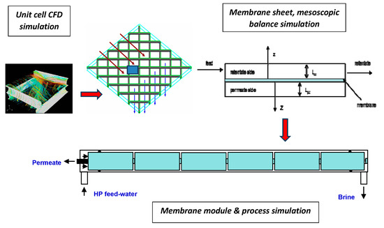
Figure 1.
The multiscale membrane module simulation approach.
In parallel, regarding membrane-material properties, it has been found that the RO membrane permeability is not uniform throughout a membrane sheet, but it can significantly vary with a characteristic length that could be even on the order of a few centimeters [15]. Very recently it has been also shown that disc-shaped ultrafiltration membrane samples (of active area 12.7 cm2) can exhibit a relatively large variation of their permeability [16]. The non-uniform permeability behavior and the related effect on the fouling layer development have not been considered so far in modeling and simulation of membrane operation. However, the impact of membrane permeability on the uniformity of fouling layer thickness can be very significant, since the respective non-uniformity seems to be larger than that due to trans-membrane pressure variation (already considered [13,17]). Therefore, the scope of this work is to analyze the effect of the spatial variation of membrane permeability on the morphology of the evolving organic fouling layer. Recently, the concern about issues dealt with in this paper, and in particular about membrane (non-uniform) permeability effects on fouling, is growing because of the novel high permeability membranes (e.g., aquaporin-and carbon-nanotube-based membranes) which are under development [18]. In addition to improved understanding of the aforementioned effect, a key target of this study is the development of an appropriate methodology to take into account the membrane permeability variation in existing membrane-performance computer-aided simulation tools [13,14,17], whose improvement has been systematically pursued by the authors in recent years.
2. Problem Formulation for Fouling Layer Thickness Evolution
To simplify matters (with no impact on the problem to be analyzed), a membrane module is considered with (i) negligible pressure drop in the permeate side, (ii) negligible osmotic pressure (low solute concentration) and (iii) negligible pressure drop in the retentate side (compared to the trans-membrane pressure). The resulting model can be also considered to hold “locally” on a size scale that is too small compared to the membrane-sheet scale (being of order 104 cm2) but large enough to contain considerable permeability variation. The relation between wall velocity or wall flux and trans-membrane pressure is typically given in terms of membrane flow resistance. The effect of the fouling layer or “cake”, as usually called, is to increase the flow resistance; thus [19]:
where uw is the wall flux, Rm and Rc are the clean membrane resistance and the time-dependent fouling layer/cake resistance, respectively, μ is the fluid viscosity and Δp is the trans-membrane pressure which for the present conditions is the same as the feed liquid pressure p(t). The fouling layer resistance is proportional to the deposit mass per unit surface area m; i.e., Rc = αm, where α is the specific cake resistance. Typically, α is considered to be affected by permeate flux, pressure and possibly deposit thickness [6,8]. Moreover, recent experimental studies of organic fouling layer formation in channels with spacers have shown that the results can be described by a rather simple relation between specific fouling/cake resistance α and wall flux [20]; i.e., α = γ(uw)β. This type of relation (obtained in the authors’ laboratory) greatly simplifies the mathematical analysis of fouling layer non-uniformity and will be adopted here. The analysis will be made in terms of membrane permeability (inverse of resistance) instead of membrane resistance since it facilitates handling of averages; it is noted that arithmetic instead of harmonic average must be considered.
Furthermore, it is considered that the membrane permeability is non-uniform on the membrane sheet and it is described by k(x,y) where x and y designate planar coordinates in the direction along the mean flow and normal to this flow, respectively. Summarizing the above discussion, it can be readily shown that the local wall flux is given as
The mass surface density m on the membrane is related to the fouling layer thickness h as h = m/ρf where ρf is the layer density. A simple evolution equation for h is obtained by considering that all the organic material contained in the filtered water is deposited (as the macromolecules completely follow the fluid streamlines), thus contributing to fouling layer formation:
where c is the mass concentration of depositing organic compounds in the liquid. In general, under conditions of constant-flux operation, the feed pressure tends to increase with time due to increasing fouling resistance. Its initial value (at t = 0) is designated as po. The average value of the permeability is defined as , where A is the membrane area; furthermore, the reference wall flux is defined as . Introducing the following dimensionless variables: ,, , , , the governing equation of fouling layer growth takes the form:
The above system must be solved for each location of the membrane (x,y) with initial condition H = 0. The solution of the system will yield the spatio-temporal evolution of the layer thickness H(x,y,T). It is noted that Equation (5) is implicit with respect to Uw, thus it must be solved numerically at each time step and spatial location. In case of constant pressure operation of the membrane, one can simply set P = 1 in Equation (5). In case of constant flux operation, the additional condition
is used to determine the feed pressure evolution P(T) due to fouling. This equation is just a statement that all the foulant mass entering the system contributes to the increase of fouling layer. A major simplification arises for the particular case of β = 1 (which is in the range of β values found experimentally [20]). In this case, Equation (5) can be solved analytically, leading to the following explicit equation for the layer thickness evolution:
A one-dimensional permeability profile of the form K(x) = 1 + 0.5cos(2πx) is assumed and the corresponding fouling layer evolution problem is solved for constant pressure (P = 1) and constant flux (P from condition (6)). The use of harmonic functions, as the one employed here, to represent non-uniform property or geometry variation is typical in science and engineering literature [21]. This treatment is focused on the evolution of non-uniformity of H; therefore, the evolution of the ratio H/Hm (where Hm is the average film thickness) is shown in Figure 2 and Figure 3 for operation under constant pressure and constant flux, respectively.
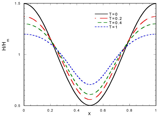
Figure 2.
Evolution of fouling layer thickness profile for a cosine variation of membrane permeability (β = 1, constant flux operation).
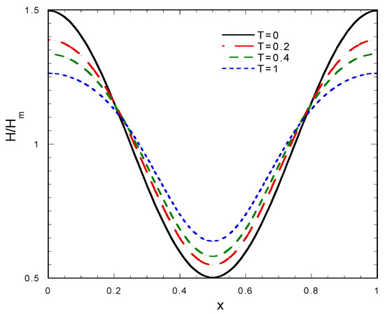
Figure 3.
Evolution of fouling layer thickness profile for a cosine variation of membrane permeability (β = 1, constant pressure operation).
In both cases the initial profile of H is similar to that of K. As the layer grows, the relative non-uniformity decreases due to the smoothing effect of H in the denominator of Equation (5). The higher the H the smaller the wall flux, leading to a self-regulation of the growing fouling layer non-uniformity. On the other hand, the quantity Uw in the denominator of Equation (5) also affects this smoothing process. The normalized profile depends mainly on the total amount of material accumulated (equivalent to Hm) which increases faster with T for constant flux, compared to constant pressure, because in the latter case the flux tends to be reduced with time. Dealing with characteristic length of K variability will be discussed in subsequent Section 5.
3. Problem Formulation for the Evolution of Thickness Probability Density Function
The above procedure of computing the fouling layer shape evolution requires many discretization points in order to cope with the shape of the function K(x,y). For example, a membrane sheet with dimensions 1 m × 1 m and characteristic area of K variation 1 cm × 1 cm needs 10,000 discretization points to be modeled. For the present simplified example, such a computational effort is acceptable. However, in case of a realistic membrane simulation, fully coupled non-linear balances must be solved for each discretization point; thus, the problem becomes computationally cumbersome [22]. To proceed, an important observation is that the fouling layer evolution model is non-topological; i.e., the thickness evolution at one point is independent of the shape of the fouling layer in its neighborhood. This means that the fouling layer, and its evolution, can be described by its probability density function (PDF) instead of its detailed shape. In the same spirit, very recently, the use of the PDF of mass transfer coefficient (computed by CFD codes) is proposed for the computation of permeate concentration without incorporating wall flow in CFD simulations [23]. Dealing with the evolution of PDF is computationally much easier than with the evolution of the detailed layer shape. Therefore, to proceed, the permeability distribution K(x,y) is described through its probability density function g(K). The physical meaning of this function is that the fraction of the membrane surface having permeability between K and K + dK is g(K)dK. By definition, and considering that K is a normalized variable, one obtains:
The lower bound of integral K = 0 denotes a completely impermeable region of the membrane. The upper bound K = ∞ denotes a kind of rupture in the membrane and for any practical purpose g(K) goes to zero as K goes to infinity; thus, the upper bound in the integrals is retained only for generality (instead of truncating at a finite value). Furthermore, the function H(K,t) is introduced describing the local thickness evolution at a location with permeability K. The equation governing dynamics of this function is
In the following, the focus will be on the case β = 1 (i.e., for specific resistance α = γuw) that allows more explicitly derived model equations; then, Equation (9) takes the form:
The average thickness Hm is computed by integrating over the permeability PDF:
The quantity of interest here is the PDF of fouling layer thickness f(H). The fraction of membrane surface covered by layer of thickness between H and H + dH is f(H)dH. The function f(H) can be constructed at each time step using the functions H(K) and g(K) as:
The discretization points, in this case, are determined by the need to sample the function g(K) and to construct H(K). Their number can be a few decades instead of thousands needed to follow the detailed shape evolution. The initial condition for the model is H(K) = 0; additionally, for the constant pressure case P = 1, whereas for constant flux the pressure evolution must be determined from the following condition, which must hold always (i.e., for every T value).
To demonstrate this approach, a membrane is considered with uniformly distributed permeability between 80% and 120% of its average value. The evolution of the PDF of H for the case of constant flux is shown in Figure 4. The way of reading this figure is the following: for a particular value of H in horizontal axis, the corresponding probability of existence appears in vertical axis. As time proceeds, the existing values of H increase and the PDF appears to broaden; however, this picture is misleading. In order to assess the evolution of the morphology, the normalized thickness H/Hm and the corresponding PDF should be considered (i.e., the same approach followed in presenting layer shape in Figure 1 and Figure 2). The evolution of the PDF of the variable H/Hm, under the same conditions as those of Figure 4, is shown in Figure 5. Initially, the PDF of H/Hm is the same with the PDF of K. As time proceeds the PDF starts narrowing. This is due to the fact that the growth rate is not the same for all H; actually it decreases with increasing H, so there is an accumulation of material (i.e., increase of layer thicknesses) in a smaller region of H/Hm followed by reduction of the spread of the corresponding PDF. The shape of the PDF also varies in time. The initial uniform distribution evolves to one with higher probability at its upper edge. This shape is also due to the reduction of growth rate as H increases, leading to probability accumulation in the region of high H/Hm values.
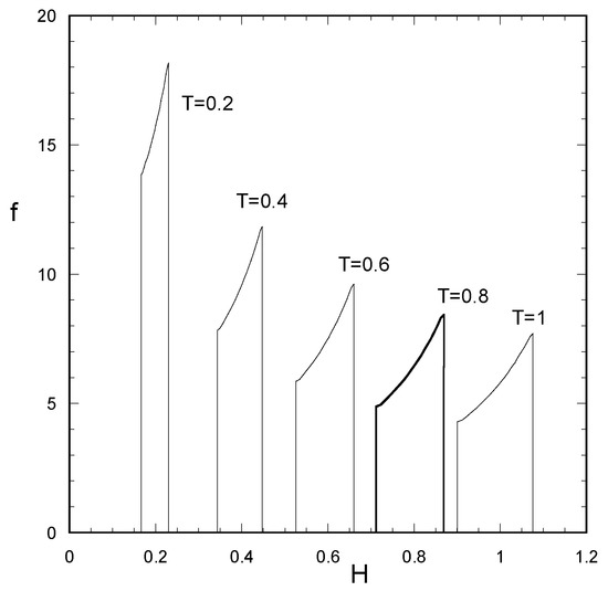
Figure 4.
Evolution of probability density function f of the fouling layer thickness H for uniformly distributed permeability between 0.8 and 1.2. (β = 1, constant flux operation).
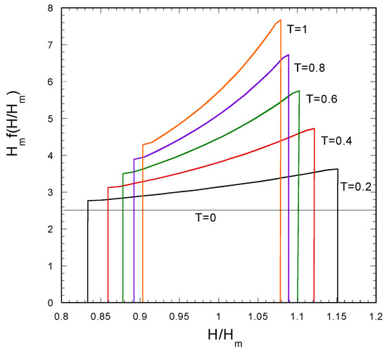
Figure 5.
Evolution of the probability density function of the normalized fouling layer thickness H for uniformly distributed permeability between 0.8 and 1.2. (β = 1, constant flux operation).
A Special Result: Small H First Order Perturbation Solution
To get additional analytical insight into the problem of thickness-PDF evolution, a first order perturbation expansion (small H limit) will be dealt with. The perturbation will be with respect to the basic solution with Uw = PK and H = PKT, resulting from Equations (4) and (5) in the limit H→0. Let us consider that
where the prime denotes the first-order correction term. Replacing in Equation (5) and taking the Taylor expansion of the denominator leads to
Taking the Taylor expansion of the power term, and retaining only the dominant term for the primed flux, leads to
Keeping only the zeroth and first order expansion terms of Uw leads to the following evolution equation for H:
In the particular case of constant pressure (i.e., P = 1) the above differential equation can be solved analytically leading to
Keeping in mind that the analysis refers to first order correction in H (so, based on the zero order solution, KT is also small) and given that K is of order unity, the above exponential can be expanded to give
Substitution of this result in Equation (12) leads, after some algebra, to the following first order analytical solution for the evolving PDF of H
Furthermore, Fi and Gi define the i-th moments of the functions f and g, respectively; i.e.,
Substitution of the relation (20) into the equation for the moments Fi leads to:
Fo = 1
The standard deviation σf of the layer thickness is given as
Substituting in Equation (25) the relations for Fi, expanding with respect to T and retaining only the first two terms, leads to
where σg = (G2-1)1/2 is the standard deviation of the permeability. Consequently, the standard deviation of the layer thickness increases in proportion to the standard deviation of the permeability, whereas the retarding effect of the denominator of Equation (5) is expressed through the coefficient . To demonstrate the effect of β and of the spread of the permeability distribution on retarding the non-uniformity of layer thickness distribution, a uniform shape of g between K = 1 − ε and K = 1 + ε will be considered. The value of ε is between 0 and 1 and denotes the spread of the permeability distribution. Replacing in equation for Cf leads to
In Figure 6, the coefficient Cf is shown as a function of ε, for three values of β. As expected, the retardation coefficient tends to increase with increasing spread of the permeability distribution (leading to spread of wall fluxes). It is interesting that Cf also increases with the exponent β. This can be explained by observing that the larger the β the larger the dampening of the permeability nonuniformity by wall flux. It is noted that Equation (26) resulted from a first order perturbation expansion, thus it holds for T much smaller than one.
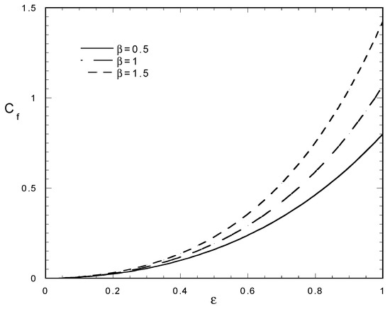
Figure 6.
Retardation factor Cf of the first order perturbation model versus permeability spread factor ε for several values of the exponent β in fouling model.
4. Effect of Concentration Polarization on Thickness Uniformity
The approach presented herein can be generalized to include additional phenomena such as the concentration polarization [24] and the cake enhanced concentration polarization [25,26]. Let us consider that the bulk concentration of the solute is non-negligible (in terms of osmotic pressure) and in the examined region of the module it is equal to cb. The wall concentration in this region (assuming complete solute rejection) will be , where kmt is the mass transfer coefficient. In the presence of spacers, the exponent in the above relation is much smaller than one [12], so a linearization is possible; i.e., cw = cb(1 + uw/kmt). The mass transfer coefficient has contributions from two resistances in series; the first is the convective diffusion in the liquid and the second the diffusion through the fouling layer (i.e., the so-called “cake” enhanced polarization). In particular, where kmto is the liquid side mass transfer coefficient and De is the effective solute diffusivity in the fouling layer. Summarizing, the relation for wall flux takes the form:
A non-dimensionalization different than the previous one will be introduced here. The constant pressure case is examined, so p is constant and equal to po. The reference flux is uwo = K(po − Γcb)/μ. The other dimensionless variables are as before. The dimensionless equation for the flux is:
where E = Γcb/(po − Γcb), Z = uwo/kmto, . A typical value of Z for a spiral wound module equal to 0.2 will be assumed here in order to demonstrate the effect of dimensionless osmotic coefficient E, and of dimensionless diffusivity in the fouling layer Δ, on fouling layer uniformity evolution. The particular case β = 1 will be considered that allows a closed form solution for the wall flux:
The distribution of permeability is the same as in the previous case (i.e., uniform between 80% and 120% of its average value). The probability density function of the variable H/Hm at the moment T = 1 for several combinations of the parameters E and Δ are presented in Figure 7. The case E = 0 corresponds to the absence of concentration polarization. The smoothing effect of concentration polarization on evolution of non-uniformity of layer thickness is evident. The explanation is that the thicker the film, the greater the “cake” enhanced concentration polarization and the smaller the wall flux leading to reduction of non-uniformity. As expected, the tendency of concentration polarization to promote uniformity of the film thickness tends to increase with increasing osmotic coefficient (E) and with decreasing diffusivity in the fouling layer (Δ). Thus, the scope of the present section is to indicate/demonstrate that the proposed simulation approach (in a generalized sense and not with particular details considered here) using PDF can be employed for any fouling layer growth model and not only for the simplest one considered in the preceding sections.
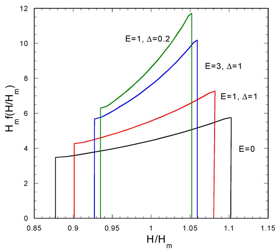
Figure 7.
Probability density function of the normalized fouling layer thickness H for uniformly distributed permeability between 0.8 and 1.2 at time T = 1, for several values of the concentration polarization related parameters E and Δ (β = 1, constant pressure operation).
5. Discussion
A key issue here is how the spatial variation of the membrane permeability can be dealt with in the current multiscale framework of modeling membrane operation [13]. The smallest scale of the analysis is that of unit cell; i.e., a periodic unit of the spacer pattern [12]. This is the finest scale for which variation can be considered. If the spatial distribution of permeability is exactly known, a direct discretization is possible. However, this information is typically not available, and it can be replaced by the probability density function of the permeability. The length scale of membrane sheet cannot be treated with the techniques presented here, since there are topological contributions to the film evolution (due to variation of transmembrane pressure) in addition to the non-topological ones (due to non-uniform permeability). The permeability variation can be treated in a statistical way; i.e., values assigned randomly, from the prevailing permeability PDF, to domains of the membrane. This technique has been used to simulate the non-uniform spatial distribution of the hollow fibers in dealing with fluid dynamics in devices like hemodialyzers [27,28]. The question is, which will be the characteristic size of regions considered to be of uniform permeability? One might consider using the small unit cell scale (1 cm × 1 cm) but then the computational load to simulate the whole sheet would be unnecessarily high. The recommendation here is the use of a coarse grid to capture the topological variation of fouling layer thickness (and also the large-scale permeability variation) combined with a subgrid non-topological handling in terms of a PDF for each mesh region. This approach bears similarities to the large eddy simulation technique for turbulence flow analysis [29]. The subgrid analysis can be implemented with the techniques presented here; i.e., at each time step and at each discretization point the probability density function distribution of thickness has to be determined by considering several permeability values and their PDF. If, instead of its complete PDF, only the average values and standard deviation of thickness are of interest (i.e., similarly to the well-known methods of moments in population balance literature [30]), the number of considered permeability values can be minimized by their appropriate choice. For example, in the case of Gaussian permeability PDF, the normalized zeros of corresponding Hermite polynomials is the optimum choice [31]. The proposed approach allows the handling of high-resolution non-uniformities in membrane permeability and fouling layer thickness without a considerable increase of the computational load of the existing simulation approaches. This approach can be also extended to the modeling of other membrane processes (e.g., membrane distillation [32]) that exhibit the same non-uniformity problems. It is important to clarify that the present work refers to intrinsic non-uniformities of the membrane itself. Their computational treatment is important not only for the fouling process but also for the clean membrane operation. The organic fouling is deterministic since it is convection dominated. Not only it does not produce non-uniformities, but it also smears out the intrinsic membrane permeability non-uniformity as it is shown above. On the opposite, biofouling is a highly stochastic process that creates non-uniformities even for an otherwise uniform membrane. This type of fouling associated non-uniformities have been treated in detail in [33] regarding their effect of membrane permeate flux. Three models for the computation of this flux are assessed in [33] and it was found that the preferred one that combines accuracy and simplicity is the so-called 1-d model which is equivalent to the model used here (i.e., Equations (2) and (3)) for the flow through the fouled membrane.
6. Conclusions
This study deals with the problem of evolution of organic fouling layer spatial non-uniformity during operation of spiral wound desalination-membrane modules. A new approach to model fouling layer thickness evolution is proposed. Two types of non-uniformities are considered; i.e., topological (induced by trans-membrane pressure variation) and non-topological (induced by membrane permeability variation). The latter can be simulated through the use of probability density functions. Several results are presented indicating the tendency for self-regulation of the fouling layer (toward uniform spatial distribution) during its growth. A methodology is suggested for the dynamic simulation of fouling layer evolution at the membrane sheet scale, which is based on a coarse grid to account for topological thickness non-uniformity combined with a subgrid treatment of non-topological non-uniformities. The results of this work are considered a necessary building block in the systematic efforts aiming to develop reliable simulators of membrane-desalination processes; incorporation of these results in an existing general modeling framework is the next step.
Author Contributions
Conceptualization, M.K. and A.K.; methodology, M.K. and A.K; software, M.K and A.K.; validation, M.K. and A.K.; formal analysis, M.K.; investigation, M.K. and A.K.; writing—original draft preparation, M.K.; writing—review and editing, A.K.
Funding
This research received no external funding.
Conflicts of Interest
The authors declare no conflict of interest.
List of Symbols
| Symbols | Explanation |
| A | membrane surface area |
| c | mass concentration of the foulant in liquid |
| cb | bulk concentration of solute |
| Cf | coefficient arising in Equation (26) for σf |
| cw | wall concentration of solute |
| De | effective diffusivity of solute in fouling layer |
| E, Z, D | dimensionless parameters |
| Fi | i-th moment of function f |
| g | probability density function of K |
| Gi | i-th moment of function g |
| H | dimensionless fouling layer thickness |
| h | fouling layer thickness |
| Hm | dimensionless average fouling layer thickness |
| K | dimensionless membrane permeability |
| k | membrane permeability |
| km | average membrane permeability |
| kmt | mass transfer coefficient |
| m | fouling layer mass per membrane unit area |
| p | pressure difference at the membrane |
| P | dimensionless pressure |
| Rc | fouling layer flow resistance |
| Rm | clean membrane flow resistance |
| T | dimensionless time |
| t | time |
| uw | liquid flux through the membrane wall |
| Uw | dimensionless wall flux |
| x,y | cartesian coordinates system on membrane surface |
| α | specific resistance of fouling layer |
| γ,β | parameters of the constitutive law relating α to uw |
| Γ | osmotic pressure coefficient |
| ε | parameter in assumed shape of function g |
| μ | liquid viscosity |
| ρf | liquid density |
| σf | standard deviation of dimensionless fouling layer thickness |
| σg | standard deviation of dimensionless permeability distribution |
References
- Karabelas, A.J. Key issues for improving the design and operation of spiral-wound membrane modules in desalination plants. Desalin. Water Treat. 2014, 52, 1820–1832. [Google Scholar] [CrossRef]
- Tang, Y.; Chong, T.H.; Fane, A.G. Colloidal interactions and fouling of NF and RO membranes: A review. Adv. Colloid Interface Sci. 2011, 164, 126–143. [Google Scholar] [CrossRef] [PubMed]
- Yiantsios, S.G.; Sioutopoulos, D.C.; Karabelas, A.J. Colloidal fouling of RO membranes: An overview of key issues and efforts to develop improved prediction techniques. Desalination 2005, 183, 257–272. [Google Scholar] [CrossRef]
- Hasson, D.; Drak, A.; Semiat, R. Inception of CaSO4 scaling on RO membranes at various water recovery levels. Desalination 2001, 139, 73–81. [Google Scholar] [CrossRef]
- Schaefer, A.I.; Fane, A.G.; Waite, T.D. Nanofiltration of natural organic matter: Removal, fouling and the influence of multivalent ions. Desalination 1998, 118, 109–122. [Google Scholar] [CrossRef]
- Sioutopoulos, D.; Karabelas, A.J.; Yiantsios, S.G. Organic fouling of RO membranes: Investigating the correlation of RO and UF fouling resistances for predictive purposes. Desalination 2010, 261, 272–283. [Google Scholar] [CrossRef]
- Vrouwenvelder, J.S.; Graf von der Schulenburg, D.A.; Kruithof, J.C.; Johns, M.L.; van Loosdrecht, M.C.M. Biofouling of spiral-wound nanofiltration and reverse osmosis membranes: A feed spacer problem. Water Res. 2009, 43, 583–594. [Google Scholar] [CrossRef] [PubMed]
- Karabelas, A.J.; Sioutopoulos, D.C. New insights into organic gel fouling of reverse osmosis desalination membranes. Desalination 2015, 368, 114–126. [Google Scholar] [CrossRef]
- Fimbres-Weihs, G.A.; Wiley, D.E. Review of 3D CFD modelling of flow and mass transfer in narrow spacer-filled channels in membrane modules. Chem. Eng. Process. Process. Intensif. 2010, 49, 759–781. [Google Scholar] [CrossRef]
- Karabelas, A.J.; Kostoglou, M.; Koutsou, C.P. Modeling of spiral wound membrane desalination modules and plants—Review and research priorities. Desalination 2015, 356, 165–186. [Google Scholar] [CrossRef]
- Kostoglou, M.; Karabelas, A.J. On the fluid mechanics of spiral wound membrane modules. Ind. Eng. Chem. Res. 2009, 48, 10025–10036. [Google Scholar] [CrossRef]
- Koutsou, C.P.; Yiantsios, S.G.; Karabelas, A.J. A numerical and experimental study of mass transfer in spacer-filled channels: Effects of spacer geometrical characteristics and Schmidt number. J. Membr. Sci. 2009, 326, 234–251. [Google Scholar] [CrossRef]
- Kostoglou, M.; Karabelas, A.J. Dynamic operation of flat sheet desalination-membrane elements: A comprehensive model accounting for organic fouling. Comput. Chem. Eng. 2016, 93, 1–12. [Google Scholar] [CrossRef]
- Kostoglou, M.; Karabelas, A.J. A mathematical study of the evolution of fouling and operating parameters throughout membrane sheets comprising spiral wound modules. Chem. Eng. J. 2012, 187, 222–231. [Google Scholar] [CrossRef]
- Mitrouli, S.T.; Karabelas, A.J.; Isaias, N.P. Polyamide active layers of low pressure RO membranes: Data on spatial performance non-uniformity and degradation by hypochlorite solutions. Desalination 2010, 260, 91–100. [Google Scholar] [CrossRef]
- Sioutopoulos, D.; Karabelas, A.; Mappas, V. Membrane fouling due to protein—Polysaccharide mixtures in dead-end ultrafiltration; the effect of permeation flux on fouling resistance. Membranes 2019, 9, 21. [Google Scholar] [CrossRef] [PubMed]
- Koutsou, C.P.; Karabelas, A.J.; Kostoglou, M. Membrane desalination under constant water recovery—The effect of module design parameters on system performance. Sep. Purif. Technol. 2015, 147, 90–113. [Google Scholar] [CrossRef]
- Tang, C.Y.; Zhao, Y.; Wang, R.; Hélix-Nielsen, C.; Fane, A.G. Desalination by biomimetic aquaporin membranes: Review of status and prospects. Desalination 2013, 308, 34–40. [Google Scholar] [CrossRef]
- Ruth, B.F. Correlating filtration theory with industrial practice. Ind. Eng. Chem. 1946, 328, 564–571. [Google Scholar] [CrossRef]
- Karabelas, A.J.; Sioutopoulos, D.C. Toward improvement of methods for predicting fouling of desalination membranes—The effect of permeate flux on specific fouling resistance. Desalination 2014, 343, 97–105. [Google Scholar] [CrossRef]
- Kostoglou, M.; Karabelas, A.J. Effect of roughness on energy of repulsion between colloidal surfaces. J. Colloid Interface Sci. 1995, 171, 187–199. [Google Scholar] [CrossRef]
- Kostoglou, M.; Karabelas, A.J. Mathematical analysis of the meso-scale flow field in spiral-wound membrane modules. Ind. Eng. Chem. Res. 2011, 50, 4653–4666. [Google Scholar] [CrossRef]
- Fernandez de Labastida, M.; Bernal, E.E.L.; Yaroshchuk, A. Implications of inhomogeneous distribution of concentration polarization for interpretation of pressure driven membrane measurements. J. Membr. Sci. 2016, 520, 693–698. [Google Scholar] [CrossRef]
- Lyster, E.; Cohen, Y. Numerical study of concentration polarization in a rectangular reverse osmosis membrane channel: Permeate flux variation and hydrodynamic end effect. J. Membr. Sci. 2007, 303, 140–153. [Google Scholar] [CrossRef]
- Hoek, E.M.V.; Elimelech, M. Cake-enhanced concentration polarization: A new fouling mechanism for salt rejecting membranes. Environ. Sci. Technol. 2003, 37, 5581–5588. [Google Scholar] [CrossRef] [PubMed]
- Hoek, E.M.V.; Kim, A.S.; Elimelech, M. Influence of cross flow membrane filter geometry and shear rate on colloidal fouling in reverse osmosis and nanofiltration separations. Environ. Eng. Sci. 2002, 19, 357–372. [Google Scholar] [CrossRef]
- Ding, W.; He, L.; Zhao, G.; Luo, X.; Zhou, M.; Gao, D. Effect of distribution tabs on mass transfer of artificial kidney. AIChE J. 2004, 50, 786–790. [Google Scholar] [CrossRef]
- Li, W.; Liu, J.; He, L.; Liu, J.; Sun, S.; Huang, Z.; Liang, X.; Gao, D.; Ding, W. Simulation and experimental study on the effect of channeling flows on the transport of toxins in hemodialyzers. J. Membr. Sci. 2016, 501, 123–133. [Google Scholar] [CrossRef]
- Glasgow, L.A. Transport Phenomena: An Introduction to Advanced Topics; Wiley: New York, NY, USA, 2010. [Google Scholar]
- Williams, M.M.R.; Loyalka, S.K. Aerosol Science: Theory and Practice; Pergamon Press: New York, NY, USA, 1991. [Google Scholar]
- Press, W.H.; Teukolsky, S.A.; Vetterling, W.T.; Flannery, B.P. Numerical Recipes: The Art of Scientific Computing; Cambridge University Press: New York, NY, USA, 1992. [Google Scholar]
- La Cerva, M.; Ciofalo, M.; Gurreri, L.; Tamburini, A.; Cipollina, A.; Micale, G. On some issues in the computational modelling of spacer-filled channels for membrane distillation. Desalination 2017, 411, 101–111. [Google Scholar] [CrossRef]
- Martin, K.J.; Bolstera, D.; Derlon, N.; Morgenroth, E.; Nerenberg, R. Effect of fouling layer spatial distribution on permeate flux: A theoretical and experimental study. J. Membr. Sci. 2014, 471, 130–137. [Google Scholar] [CrossRef]
© 2019 by the authors. Licensee MDPI, Basel, Switzerland. This article is an open access article distributed under the terms and conditions of the Creative Commons Attribution (CC BY) license (http://creativecommons.org/licenses/by/4.0/).