Experimental Study of a Gas–Liquid Flow in Vacuum Air-Lift Column Using an Optical Bi-Probe

Abstract

The vacuum airlift column process was patented in 2007 and is under development. The experimental study of its hydrodynamics is one of the axes explored to optimize its design and operation. The object of the study presented in this paper is to determine the functions of phase indicator (gas holdup, superficial gas velocity and bubble size) of the gas–liquid flow. The experimental analysis is carried out using a two-phase instrumentation consisting of an optical fiber bi-probe. The use of experimental techniques has made it possible to better understand the hydrodynamics of a two-phase flow. The optical bi-probe placed between two column flanges made it possible to have a complete mapping of the flow of the dispersed phase. The use of a mass flow meter and an ultrasonic flowmeter, in different flow configurations, provided data on the column operation.

1. Introduction

Bubble columns are industrial (process) devices that provide a mixture of a bubbly gas phase and a liquid phase. For some decades, studies carried out on this device contributed to the understanding of their hydrodynamics [1]. An air-lift column is a bubble column in which a partition has been introduced to channel the flow of the liquid and gaseous phases between several compartments of the column. The injection of air made into one of the compartments makes it possible to modify the apparent density and expansion of the two-phase fluid, causing the circulation of the initially immobile liquid phase [2]. Air-lift columns have been the subject of several studies in the mining and oil industry [3]; in aquaculture [2] as well as in chemical and biochemical processes [3]. The air-lift vacuum column that is the subject of this study is based on the principle of air-lift and flotation, under vacuum. The technology has been patented by the French Research Institute for the Exploitation of the Sea (IFREMER) and the National Institute of Applied Science (INSA) Lyon [4]. The column combines in its operation the functions of hydraulic pumping, solute transfer and particulate phase separation and minimizing energy costs [2]. The gas–liquid flows in these columns are intrinsically unstable and the dynamics of such flows influence the mixing and mass transfer performance of the bubble columns. It is therefore important to characterize the dynamics of the gas–liquid flow [5]. Moreover, the complete knowledge of the overall dynamics of the fluids in the bubble column rests on that of the bubbles [6]. Knowledge of bubble size distribution and gas holdup is crucial for determining interfacial gas–liquid mass transfer [7]. The analysis of the particle size of the bubbles in the columns can be is either performed by intrusive techniques, disturbing the flow or by non-intrusive techniques. Non-intrusive techniques use either tomographic probes [8,9], or image analysis by particle image velocimetry (PIV) [3,10,11,12], intrusive techniques rely on the usage of probes like fiber-optic probes, etc. [3]. In terms of results, intrusive techniques provide local measurements, while non-intrusive techniques provide a cross-sectional distribution with different spatial and temporal resolutions [6]. The advantages and disadvantages of different intrusive and non-intrusive techniques and their applications to multiphasic flows have been presented by several previous works [13]. Optical probes are phase detection devices that have been developed for several decades [14,15,16,17,18]. The optical probe uses the variation of the refractive index of the medium which characterizes the phase change. This is a principle that has been used for a long time for level detection and has resulted in several achievements. Optical probes are intrusive devices used very widely because of their great ease of use and the quality of the measurements obtained [19,20,21,22,23,24,25]. They have several advantages including a very fast response (less than $1\mathsf{\mu }$s for a single fiber probe), a very good spatial resolution (less than $10\mathsf{\mu }$m for a single fiber probe) and their use in a wide range of pressure and temperature [26]. Among the authors who have carried out work with the optical probe, Cartellier [14] has characterized the performance of single-fiber optical probes for measuring gas holdup. Serdula and Loewen [27] conducted a series of experiments to evaluate the feasibility of using a single-fiber optical probe to measure the gas holdup. They found that these probes could be used to perform measurements of gas holdup, bubble size and velocity. Kiambi et al. [28] evaluated the accuracy of an optical bi-probe technique to perform two-phase local flow measurements for 2.15 and 4.5 mm size bubbles. Comparing this technique with imaging, they concluded that optical probes underestimate the gas holdup from about $6\%$ to $14\%$. They also reported errors of less than $5\%$ for gas velocity up to 38 cm·s${}^{-1}$. Rojas and Loewen [20] demonstrated that single-fiber optical probes are capable of accurate and simultaneous measurements of gas holdup and bubble sizes under breaking waves. Vejrazka et al. [29] studied the mechanisms contributing to errors in optical probe measurements. Measurement errors have been reported based on a modified Webber number (M), which is the holdup of the bubble moment to the pulse of the surface tension of the probe, and characterizes the ability of the bubble to overcome the surface tension. It is reported that, in the case of M greater than 50, the gas holdup and the maximum chord measurement error should be less than $10\%$. Mizushima and Saito [30] developed a 35° angle single-fiber optical probe that generated a pre-signal when the bubble is pierced in the center, allowing differentiation between bubble detection and diameter measurement. Pjontek et al. [22] used a single-fiber optical probe to measure local bubble characteristics in a 101.6 mm diameter column operating at pressures up to 9 MPa. Aliyu et al. [25] have developed a dual optical fiber probe system for measuring the hydrodynamic characteristics of a gas–liquid flow. The gas velocity and bubble size values measured by the fiber optic probe are in line with those estimated using a photographic method using a fast camera system. In addition, the vacuum levels obtained with fiber optic probes showed good agreement with the holdup of air drawn in the two-phase mixture as measured by a flow meter. Fiber optic probes have the advantage of high sensitivity and minimal intrusion due to their micrometric size, and can be used when other instruments are difficult to deploy or do not give the temporal resolutions. The study presented in this paper consists of the determination of the phase indicator functions of two-phase flows in a vacuum air-lift column. These functions are the gas holdup, the superficial gas velocity and the particle size of the bubbles, the flow rate and the velocity of the liquid phase. The experimental analysis will be carried out using two-phase instrumentation consisting of an optical fiber bi-probe, a mass flow meter and an ultrasonic flow meter.

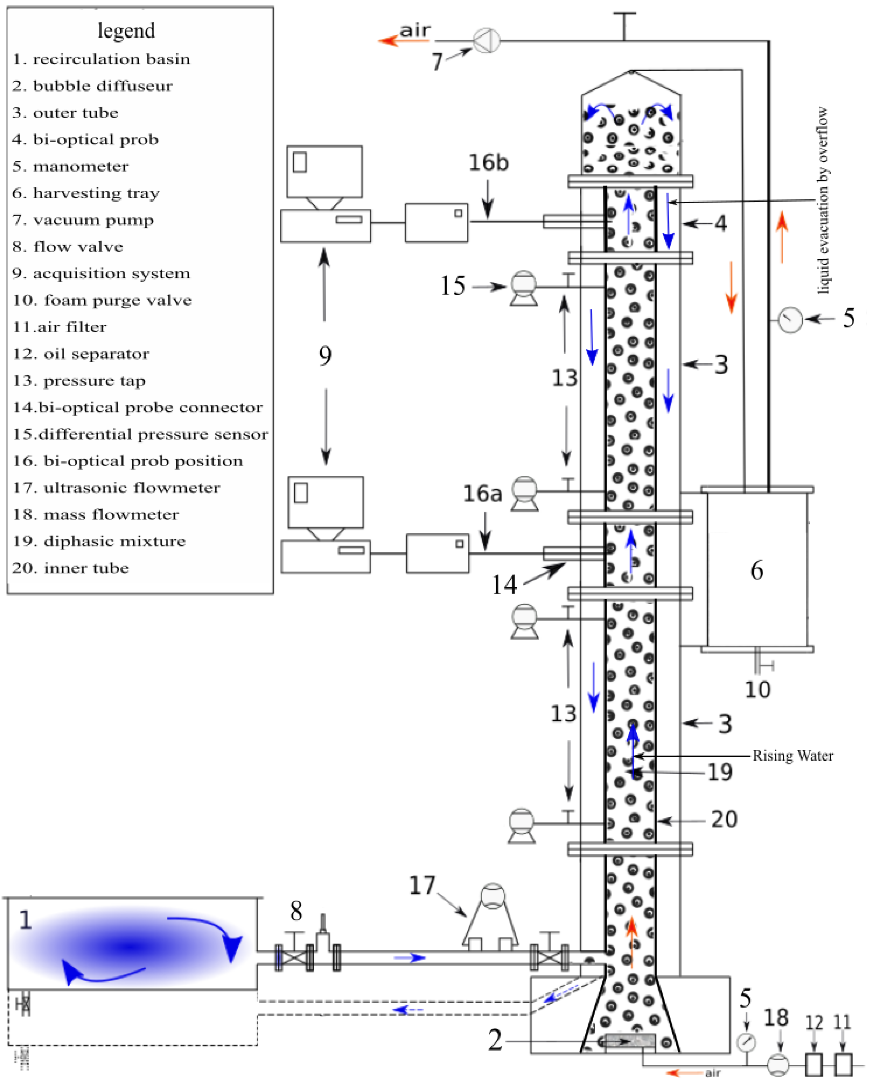
2. Materials and Methods

The experimental study of the hydrodynamics of the vacuum column was carried out on a test bench shown schematically in Figure 1 below. The system consists a vertical column (two concentric Plexiglas tubes of 80 and 150 mm diameter respectively), a storage tank and a vacuum pump. The vertical column ends with cone placed at its top and connected to a vacuum pump. The column is made of two sections of 1 m length each and a 25 mm section equipped with a plug for the optical bi-probe. Its base is equipped with a ceramic bubble diffuser and connected to a water recirculation basin. This basin is connected to the column by two parallel 50 mm diameter PVC pipes. A suction pipe connected to the inner tube and a discharge pipe, to the outer tube. A harvesting tank which acts as a suction chamber of the vacuum pump and a collection tank for the particles trapped by the bubbles is appended to the air-lift column. The injection of air is made in the central tube at the bottom of the column through the ceramic bubble diffuser. The compressed air used is that of the collective air supply system of the laboratory. It is supplied under a maximum pressure of 6 bar. A pneumatic circuit has been designed for our device in order to be able to filter the air and to control its pressure using a pressure switch. The compressed air is filtered and then passed through a pressure switch before entering a mass flow meter to record the effective air flow for the air-lift. Tap water is used at room temperature; distilled water will alternatively be used. The liquid flow rate of the air-lift is measured by an ultrasonic flow meter. An optical bi-probe equipped connected to an acquisition system is inserted into the inner tube of the column in order to characterize the gas phase. The air injection causes an air lift effect that draws water from the recirculation basin and drives it upward into the central tube. At the top of the central tube, the water flows into the peripheral ring and goes down to the recirculation basin. The vacuum pump allows for putting the column under vacuum which raises the water level in the column and the maintenance above the inner tube to allow the hydraulic circulation. The characterization of the continuous (liquid) phase flow was made using an ultrasonic flowmeter. Bubble flow was characterized by two-phase instrumentation consisting of an optical bi-probe, an optoelectronic module, an oscilloscope, and an acquisition and processing unit. A global study of the hydrodynamics of the differential pressure sensors is made before the study by optical bi-probe. Differential pressure sensors are used to determine global parameters: pressure and holdup. The density of the gas is defined from the pressure at mid-height of the column.

2.1. Local Gas Holdup

The local gas holdup is directly obtained by dividing the total time ($\sum {\tau }_i$) of presence of the gas phase in contact with the sensitive tip of the optical probe by the full time (T) of observation. The optical bi-probe provides a gas holdup for each probe. The gas holdup at the point of measurement is obtained by the following relation:

$$\alpha =\frac{\sum {\tau }_i}{T}.$$

(1)

2.2. Bubble Rise Velocity

The bubble rise velocity is obtained by processing the signals delivered by the sensitive points of the optical bi-probe. The use of a single fiber probe does not make it possible to deduce the bubble rise velocity, which becomes possible with a bi-probe. The principle of calculating the average bubble rise velocity is quite simple: the distance separating the sensitive zones being known (gap between the probe), a measurement of the time taken by the interface to pass from one to the other leads to the estimate velocity by the expression:

$$v=\frac{d}{\tau }$$

(2)

with:

• v the average bubble rise velocity;
• D the distance between the tips of the bi-probe (2 mm);
• $\tau$ the time shift between the signals of the two optrodes.

2.3. Bubble Size

The phase indicator functions of the acquisition system consists of slots representing contact times of the bubbles with the optrodes of the optical bi-probe. When the rate of evolution of bubbles is known, this contact time can be directly connected to a length. The average diameter of the bubbles is determined from the local gas holdup and the interfacial area by applying the formula:

$$d_{probe}=\frac{6\alpha }{A_i}$$

(3)

where $A_i$ is the interfacial area and $\alpha$ the local gas holdup. The “average diameter” of bubbles determined by the VIN 2.0 software (RBI Instrumentaion, Meylan, France) of the optical bi-probe actually corresponds to a chord average. An equivalent diameter of bubbles is proposed in the literature. This average diameter is directly estimated from the diameter obtained at the bi-probe ($d_{probe}$) and a form factor denoted $\chi$ of the bubbles [31,32]. The expression of this equivalent diameter is given by the formula:

$$d_{eq}=K.d_{probe}.{\chi }^{2/3}$$

(4)

$d_{probe}$ is the diameter of the bubbles at the optical bi-probe; $\chi$ a form factor of the bubbles.

K is a constant often taken equal to 1.5 for spherical bubbles [15,33,34,35].

3. Results and Discussion

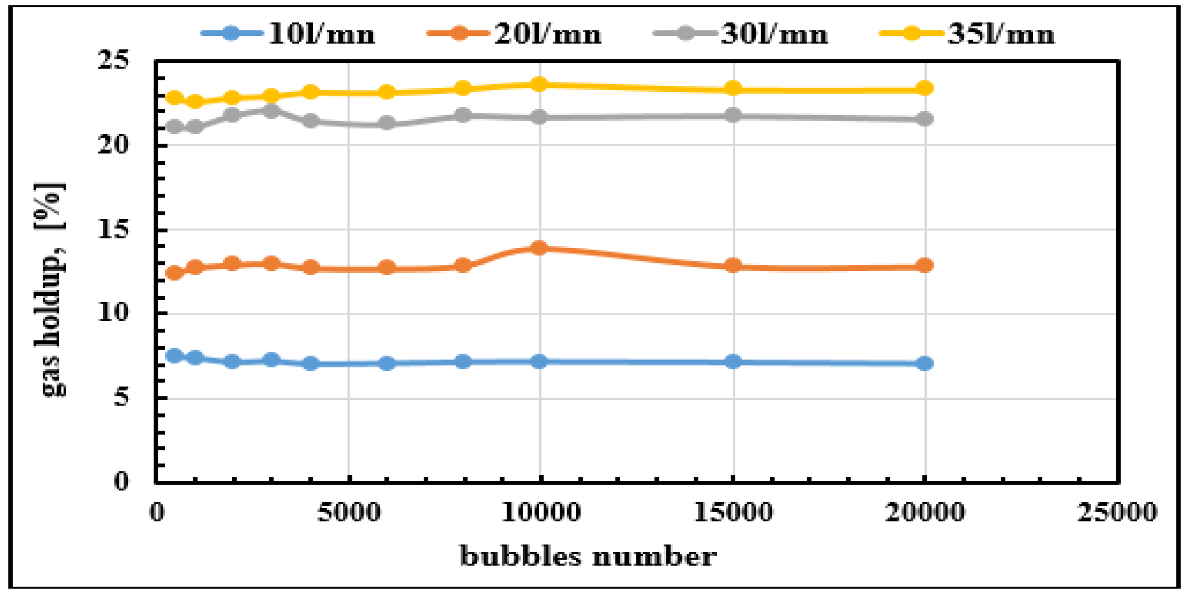
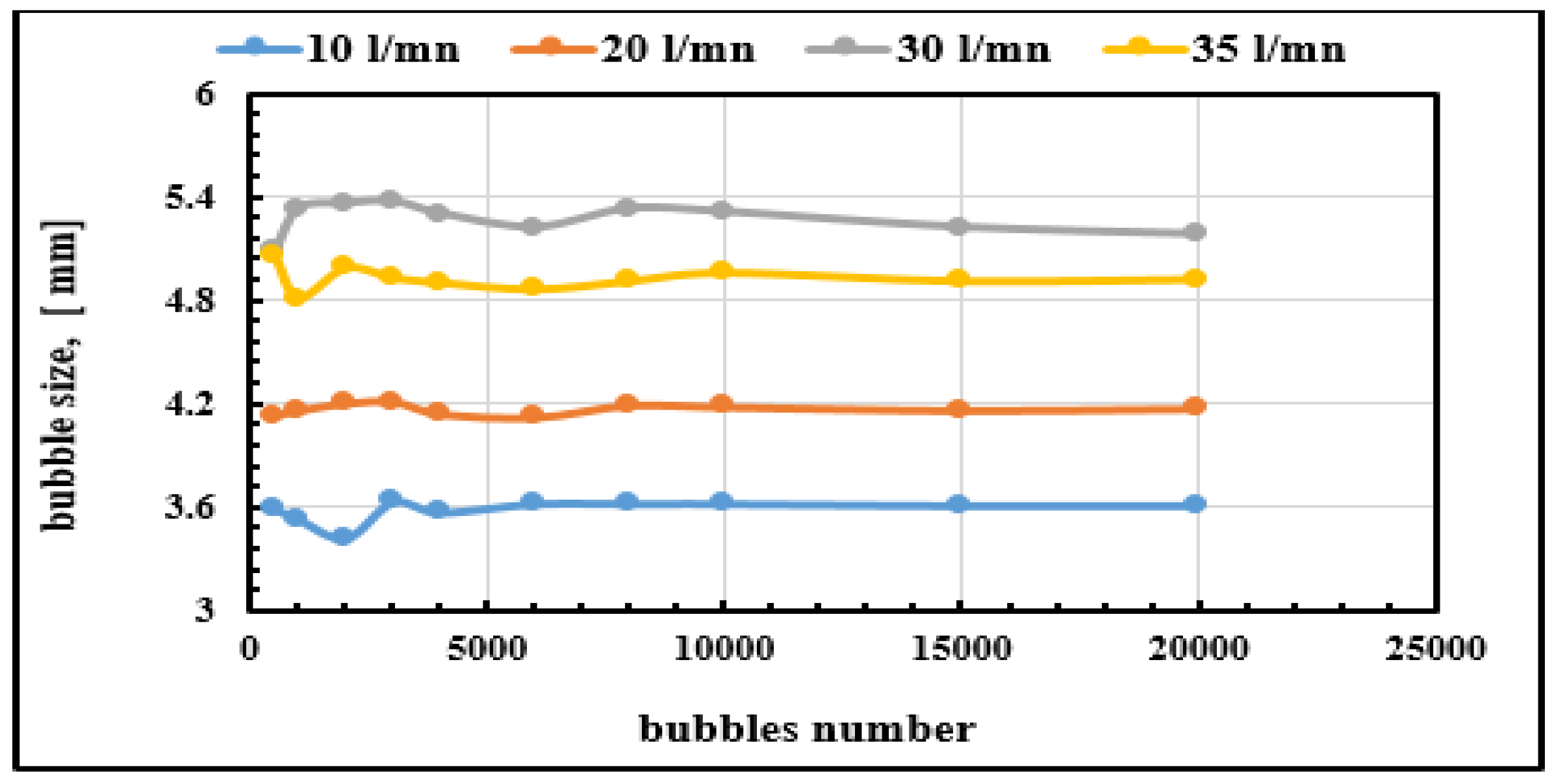
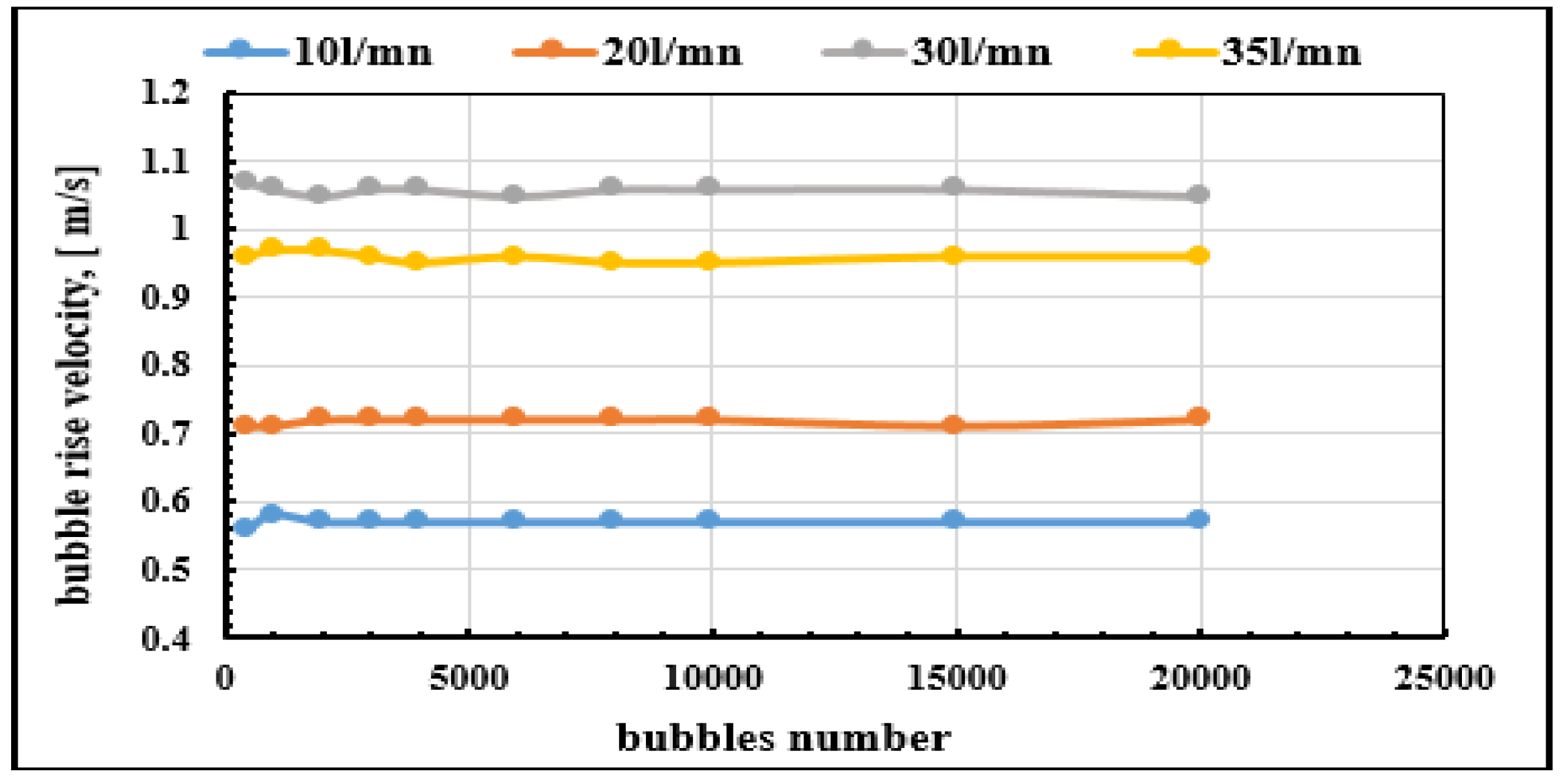
3.1. Convergence of Optical Bi-Probe Measurements

In this study, the convergences of the optical bi-probe measurements are observed as a function of the bubble number for gas holdup ${\alpha }_G$ (Figure 2), bubble size (Figure 3) and bubble rise velocity (Figure 4). The observations of convergence curves indicate that a bubble number of $1\times {10}^4$ is sufficient to guarantee at the same time the convergence of the measurements of gas velocity, bubble size and gas holdup. This result is valid for all gas flow rates.

3.2. Hydrodynamics of the Liquid Phase

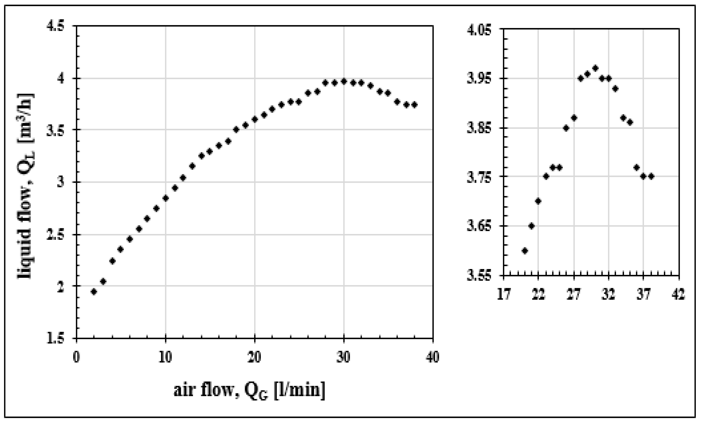
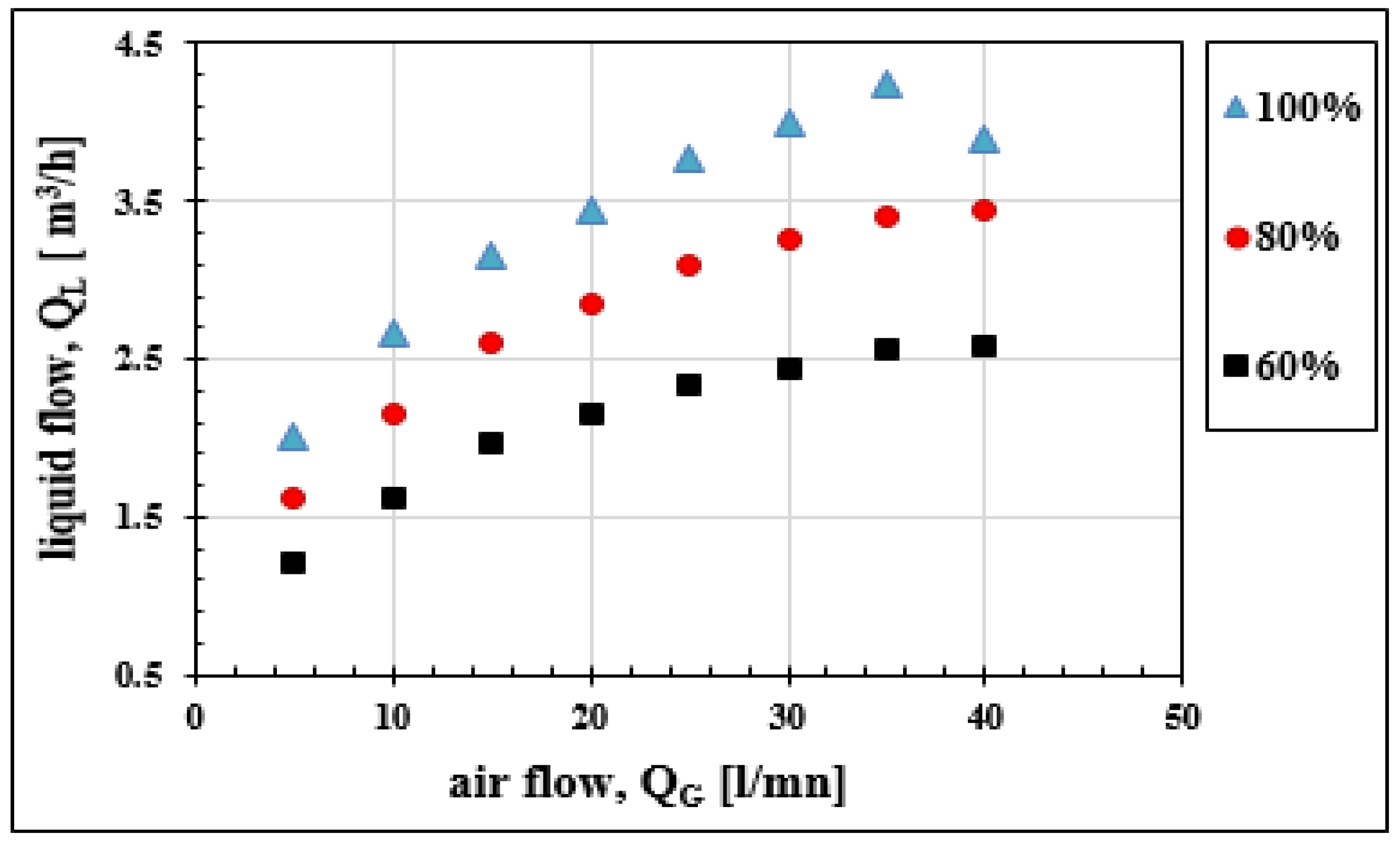
3.2.1. Analysis of the Pumping Function through the Liquid Flow

The goal is here to analyse the pumping capacities of the column. The experimental device studied is that illustrated in Figure 1. The analysis of the Figure 5 makes it possible to observe that the liquid flow rate in the air-lift column is directly proportional to the flow rate of injected air over the range from 2 to 30 L·mn${}^{-1}$. On the other hand, for air flows above 30 L·mn${}^{-1}$, we observe an inverse phenomenon on the liquid flow, with a decrease of the latter.

This phenomenon is explained by the appearance of a counter air-lift effect in the outer tube of the column materialized by the presence of air bubbles at the outer tube of the column: this slows the return of the liquid to the recirculation basin of the column and decreases the velocity of hydraulic circulation and therefore the liquid flow.

Since the liquid flow is a function of the air-lift airflow, we installed a shut-off valve on each duct connecting the column to the recirculation basin. These valves allow us to modify the liquid flow rate for a fixed air flow. In Figure 6 below, the liquid flowrate evolution at the three regimes are shown. At the first rate curve corresponding to a total opening of the valve ($Q_L=100\%$) of liquid flow, two others are added, corresponding to 80 and $60\%$ of the initial flow. The two new curves illustrate that, whatever the liquid flow rate, the pumping regime keeps the same profile with a maximum reached for an air flow of 30 L·mn${}^{-1}$.

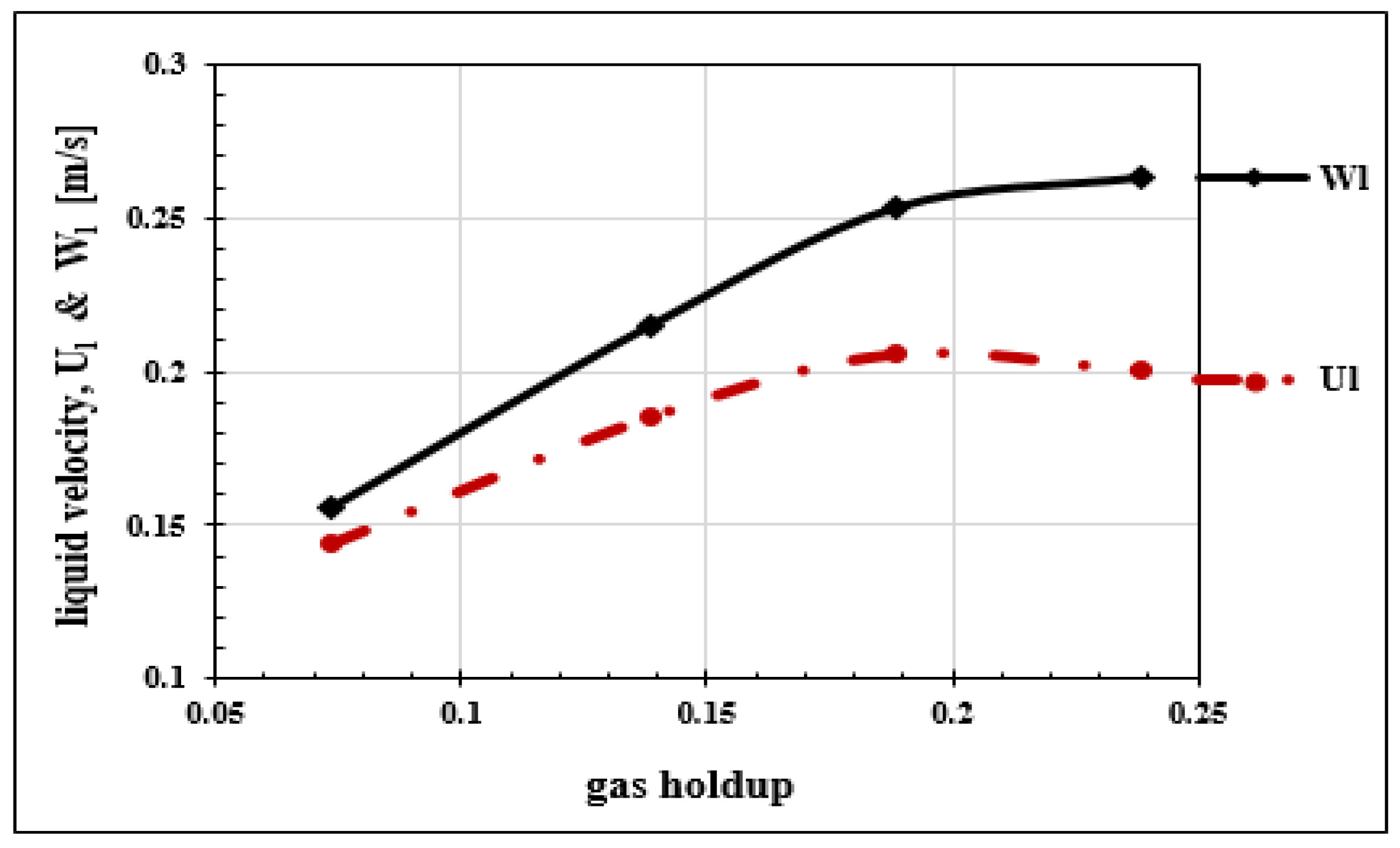
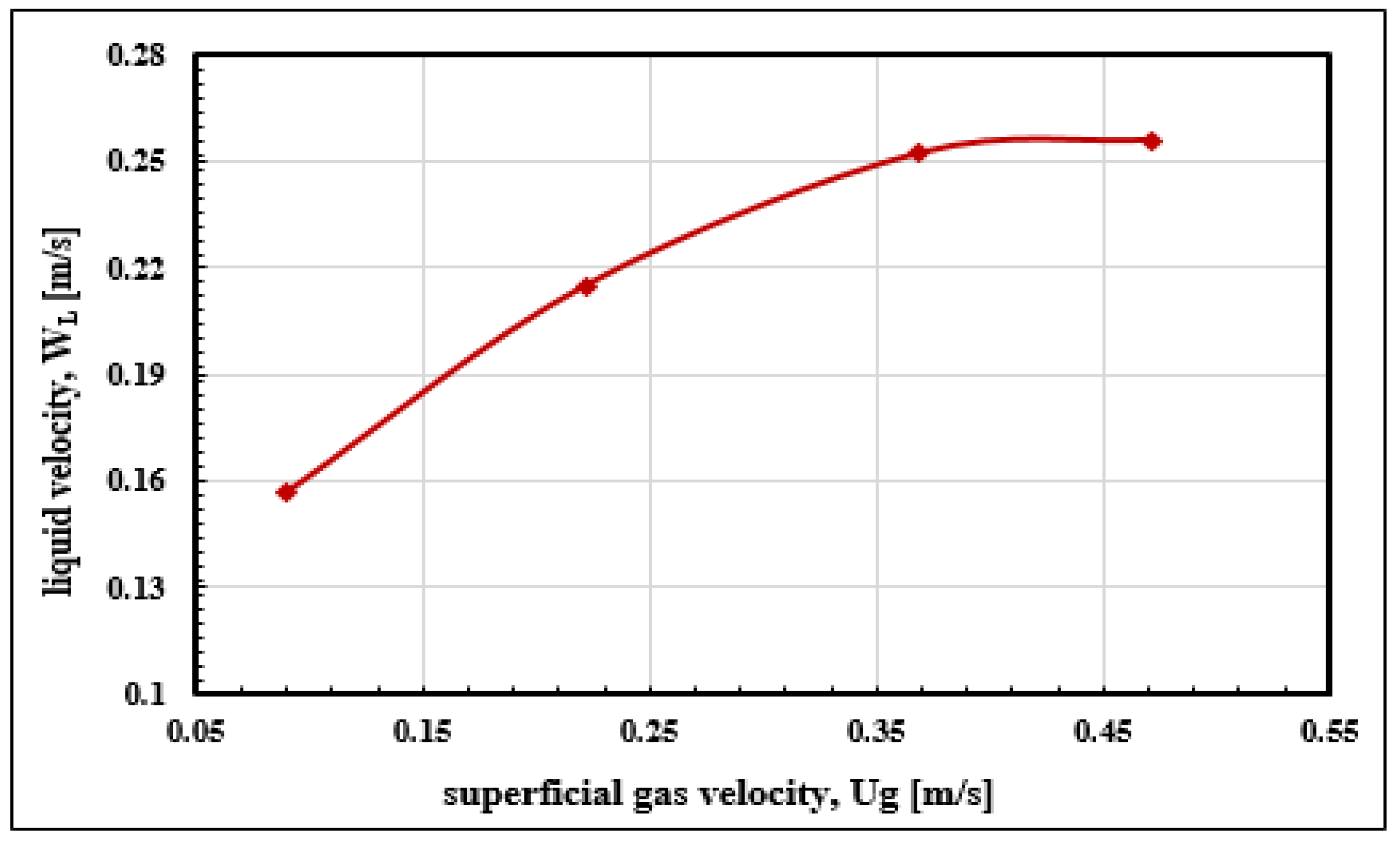
3.2.2. Analysis of the Liquid Phase Velocity

The liquid velocity of the two-phase mixture of the bubble column is initially estimated from the liquid flow obtained by direct measurement using an ultrasonic flow meter. The velocity is obtained by the following expression:

$$U_L=\frac{Q_L}{A_c},$$

(5)

where:

• $Q_L$: liquid flow measured in m${}^3·$s${}^{-1}$;
• $U_L$: liquid velocity in m·s${}^{-1}$;
• $A_c$: total section of the inner tube of the column in m${}^2$.

This first liquid phase velocity ($U_L$) does not take into account the diphasic mixture, that is to say, the presence of a gas holdup in the column. We will determine from the liquid velocity above an effective liquid velocity that takes into account the presence of a gas phase in the mixture. The actual velocity of the liquid is determined by the expression:

$$W_L=\frac{U_L}{{\epsilon }_L},$$

(6)

where:

• $W_L$: actual liquid velocity in m·s${}^{-1}$;
• $U_L$: liquid velocity in m·s${}^{-1}$;
• ${\epsilon }_L$ is the volume holdup of the air given by the expression:

  $${\epsilon }_L=1-{\alpha }_G$$

  (7)

  with ${\alpha }_G$ the gas holdup.

Figure 7 shows the two calculated velocities of water ($U_L$ and $W_L$) as a function of the gas holdup. An analysis of the two curves shows that the two velocities increase with the gas holdup reaching a threshold for a gas holdup of $19\%$. It also appears that the gap between the two velocities is widening with the gas holdup. This difference is well marked for gas holdups above $14\%$. This difference is stabilized from a gas holdup of $19\%$ where the liquid velocity $W_L$ is $25\%$ higher than $U_L$. This difference indicates the importance of knowing $W_L$ on which depend the microscopic characteristics or the local flow.

3.3. Hydrodynamics of the Dispersed Phase

The hydrodynamic study of the gaseous phase of the vacuum air lift was carried out using an optical bi-probe of the RBI brand. This instrument measures local parameters, so in the context of the present study a cartography of the flow has been made in a horizontal plane. In total, six axes or diameters are subject to local measurement. On each axis, the bi-probe measured seven points. The schematic representation of the different measurement axes of the bi-probe is shown in Figure 8.

3.4. Study of Global Parameters

Here, we define two global parameters that make it possible to characterize the hydrodynamics of the dispersed phase of the air-lift. This is the global gas holdup and the superficial gas velocity.

3.4.1. Superficial Gas Velocity

The superficial gas velocity in the air-lift column takes several expressions. We are going in a first approach to determine a superficial gas velocity. This is a global gas velocity used very often in the hydrodynamic study of bubbly flows. This superficial gas velocity is obtained from the volumetric flow and the cross sectional area of the bubble column. The superficial gas velocity is thus given by the expression:

$$U_G=\frac{Q_v}{A_c},$$

(8)

• $A_c$ is the area of the total section of the inner tube of the column m${}^2,$
• $Q_v$ is the volumetric gas flow, m${}^3·$s${}^{-1},$
• $Q_v=\frac{Q_m}{\rho },$
• $Q_m$ is the mass gas flow in m${}^3·$s${}^{-1},$

with:

• $Q_m=\frac{Q_G}{\rho },$
• $Q_G$ is the gas flow rate is obtained by direct measurement with the mass flow meter, m${}^3·$s${}^{-1},$
• $\rho$ and $\rho {}^{\prime }$: gas density (Kg·m${}^{-3}$),
• ${\rho }_G=\frac{P}{RT},$
• T: temperature,
• P: pressure.

This superficial gas velocity ($U_G$) is a linear function of the airflow. From the superficial gas velocity ($U_G$), we will determine a velocity more representive of bubbles rise velocity. This new gas velocity, denoted $W_G$, takes into account the volume fraction of the liquid (${\epsilon }_L$) itself taking into account the gas holdup (${\alpha }_G$). The bubble rise velocity $W_G$ is obtained by the expression:

$$W_G=\frac{U_G}{{\alpha }_G},$$

(9)

• ${\alpha }_G$ is the gas holdup,
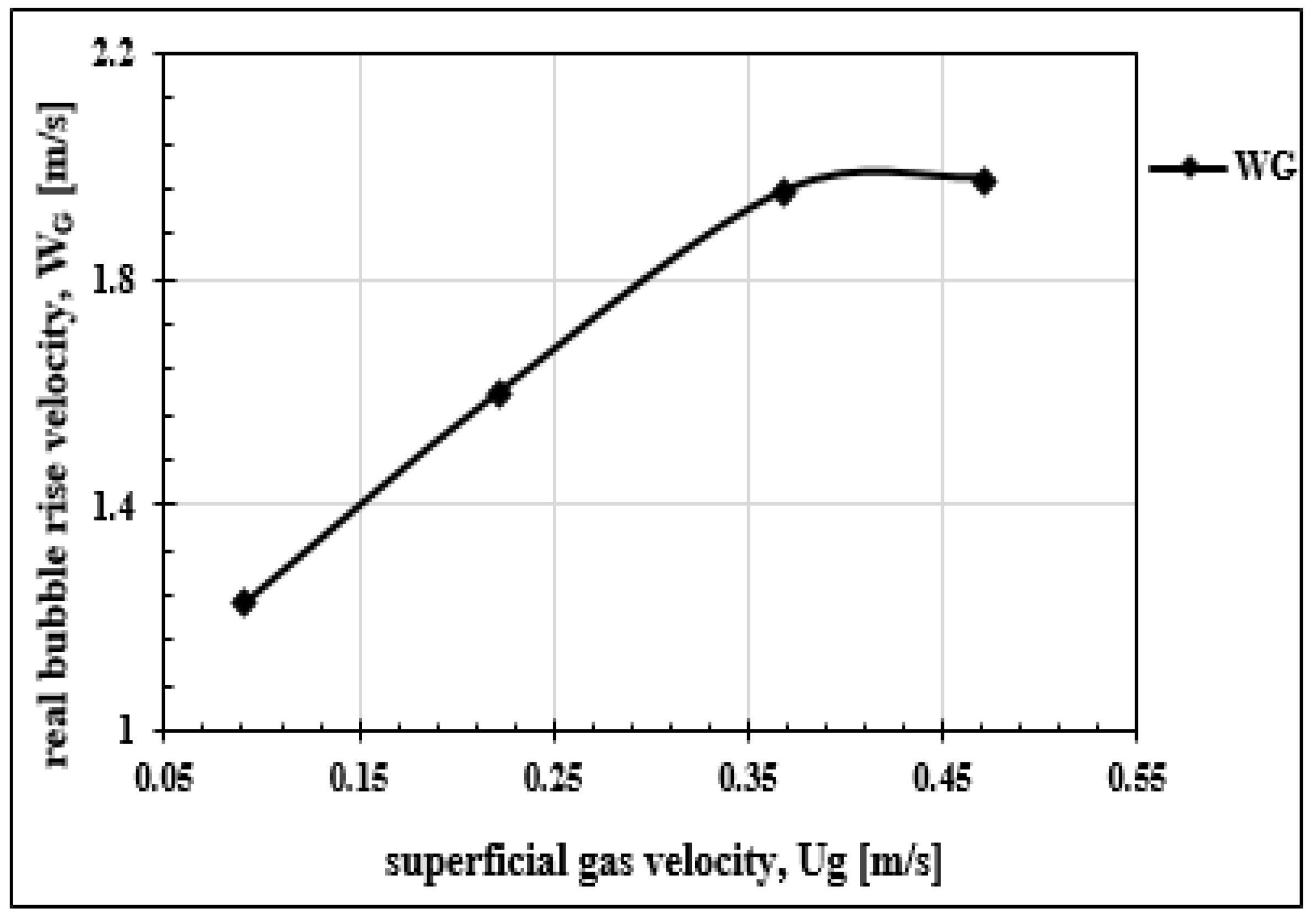
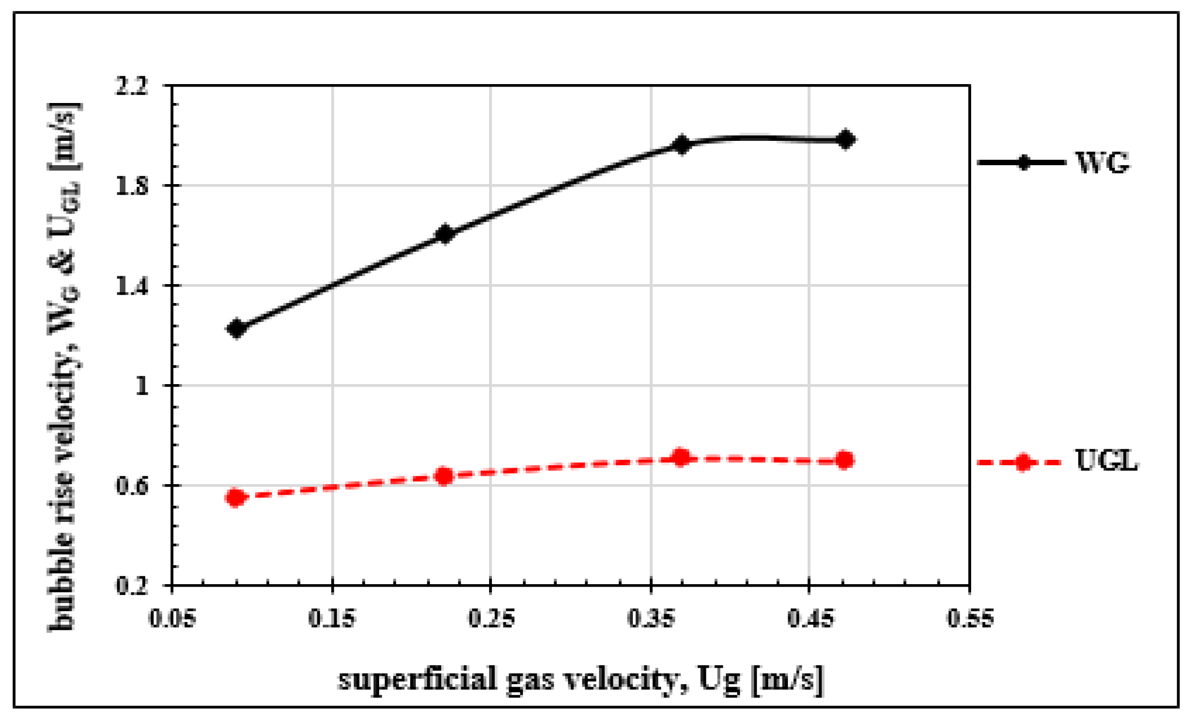
• $W_G$ is the bubble rise velocity,
• $U_G$ is the superficial gas velocity ($m.s^{-1}$).

The profile of bubble rise velocity $W_G$ as a function of the superficial gas velocity $U_G$ (Figure 9) shows that the bubble rise velocity reaches a plateau starting from a superficial gas velocity $U_G=0.36$m·S${}^{-1}$. The plot of the real liquid velocity $W_L$ as a function of the superficial gas velocity $U_G$ (Figure 10) also shows the same threshold effect for the same value of $U_G$ ($U_G=0.36$ m·S${}^{-1}$).

Knowing the real velocities of the liquid and those of the air bubbles, we can deduce the gas slip velocity ($W_{G-L}$) of the bubbles with respect to the water, by the expression:

$$W_{G-L}=W_G-W_L.$$

(10)

In Figure 11, we find that this gas velocity has the same profile as that of $W_G$ and with the same plateau starting from $U_G=0.36$ m${}^{-1}$.

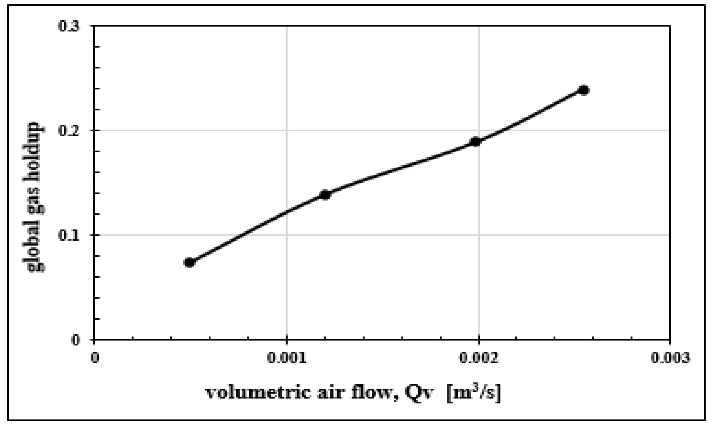
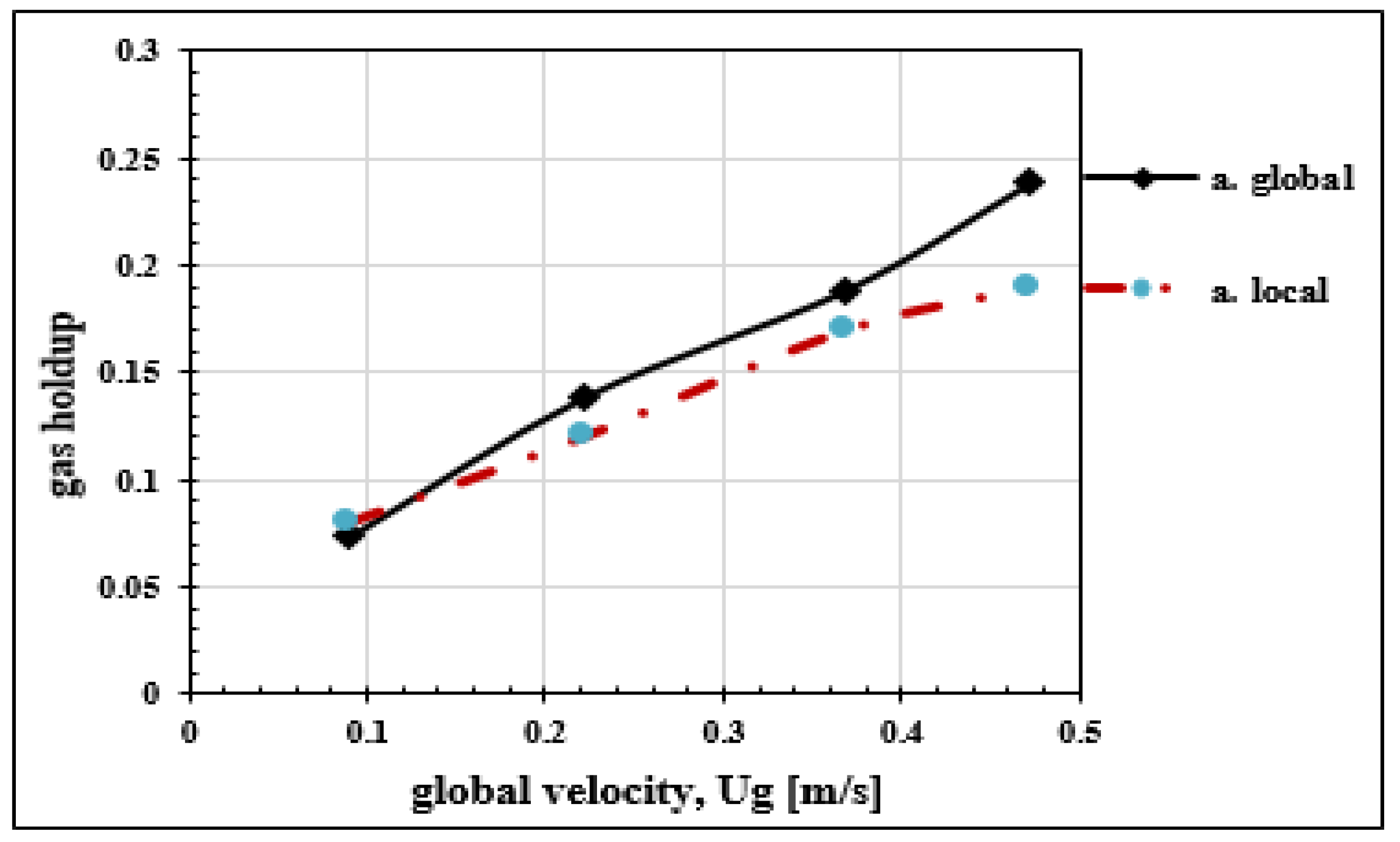
3.4.2. Global Gas Holdup

The global gas holdup is defined as the volume of dispersed gas relative to the total volume of the two-phase mixture. It is obtained by pressure measurements using the differential pressure sensors placed on the column (Figure 1). Differential pressures are measured in water height. Each air flow leads to a differential pressure measurement and therefore to a different global gas holdup. To determine the pressure variation, we made two hypotheses:

• there is conservation of gas velocity;
• the pressure losses in the column are negligible (because the wall of the Plexiglas column is smooth).

The variation of the pressure is given by the expression:

$$\Delta P={\rho }_{L}gh{\alpha }_L+{\rho }_{G}gh{\alpha }_G,$$

(11)

with:

${\alpha }_L=1-{\alpha }_G$ the volumetric fraction of the liquid we will have the expression:

$$\Delta P={\rho }_{L}gh(1-{\alpha }_G)+{\rho }_{g}gh{\alpha }_G.$$

(12)

The contribution of the mass of gas in the mixture is negligible. It is in the order of $1.13\times {10}^{-4}$ and is practically within the margin of error made by the pressure sensor. Thus, we could very well neglect the term ${\rho }_{g}gh{\alpha }_G$ in the expression of the gas holdup. We will then have the following relationship:

$$\Delta P={\rho }_{L}gh(1-{\alpha }_G),$$

(13)

$${\alpha }_G=1-\Delta P/({\rho }_{L}gh),$$

(14)

where:

• g: acceleration of gravity;
• h: mix height;
• ${\rho }_L$: density of the liquid;
• $\Delta P$: variation of the measured pressure;
• $\alpha {}_G$: global gas holdup.

The gas holdup increases with the air flow ($Q_G$) while the variation of the pressure ($\Delta P$) is inversely proportional to the same air flow. In Figure 12, the global gas holdup is represented in relation with volumetric air flow ($Q_v$); as expected, the overall gas holdup increases with the injected air flow rate and will be compared hereafter to the local gas holdup measured by the optical bi-probe as in Besagni et al. [36]. This accuracy will also depend on the difference that will be obtained between the values of the two gas holdup measurements.

3.5. Hydrodynamics Parameters by Optical Bi-Probe

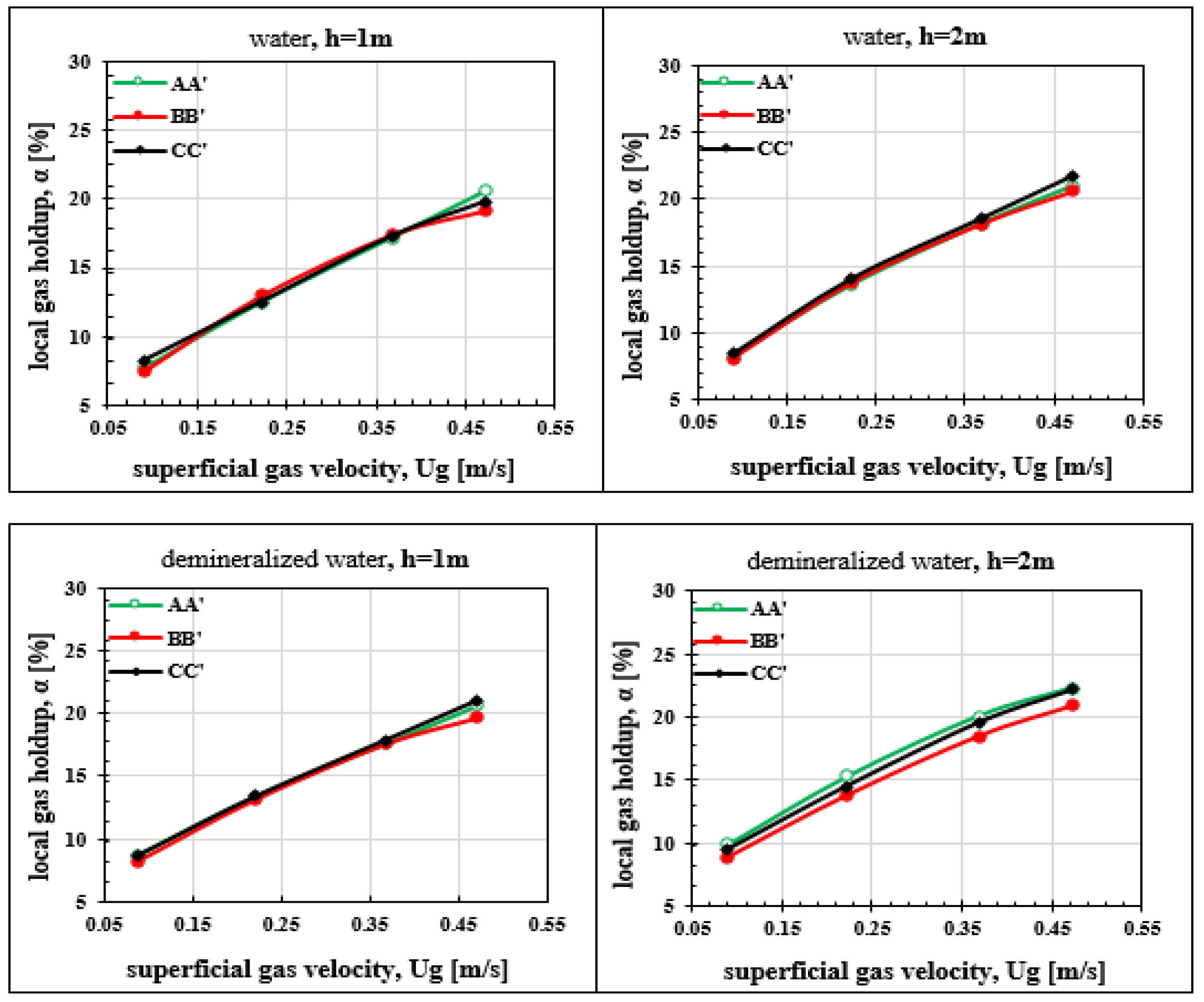
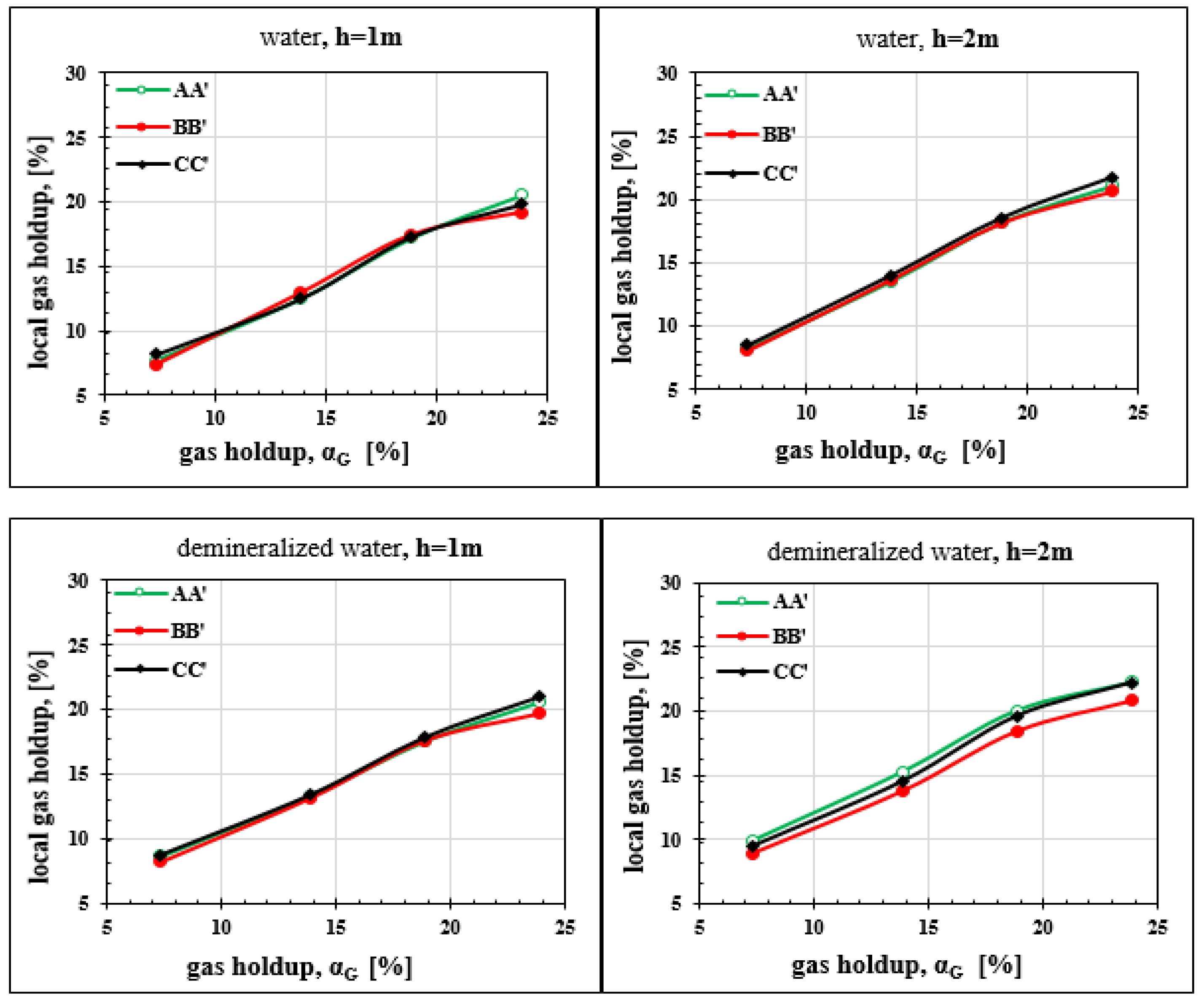
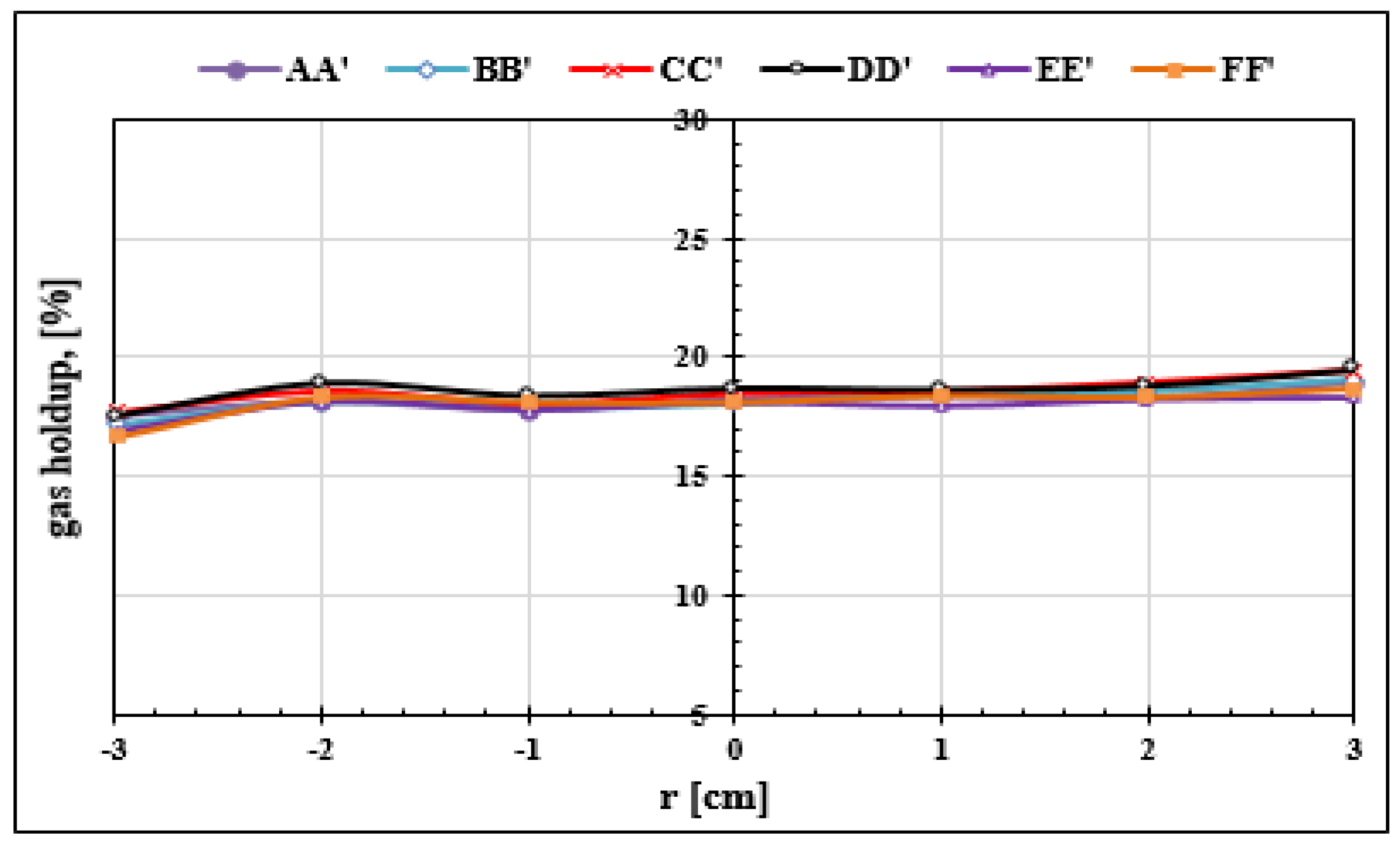
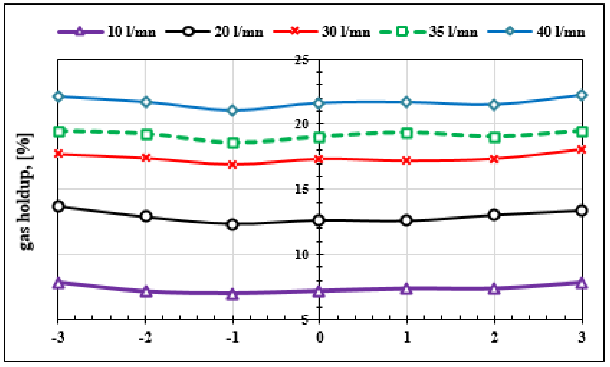
3.5.1. Local Gas Holdup

Local gas holdup is deduced from one of the two channels of the optical probe. Only one tip of the probe can be used to measure time during which it is exposed to gas and time for liquid. This measurement is made in two different sections of the column one meter apart. Measurements are carried out, first, in the presence of tap water, subsequently with demineralised water to analyze the effect of the hardness of the water on the gas holdup. The results of the various measurements illustrated in Figure 13 and Figure 14 point out that, in the configuration of our study, the hardness of water has pratically no effect on the gas holdup. The results for both types of water are very close for the first section. With demineralised water, there is a slightly higher gas holdup at 2 m. The difference is small, BB’ results are for example practically identical for both tests (nature of water). With demineralised water, a slight dissymmetry appears with a slightly higher gas holdup in AA’ and CC’. This increase in the gas holdup is explained by the phenomenon of bubble coalescence, which is more important in demineralised water. The increase of gas holdup with height has already been reported by Besagni et al. [36]. The coalescence of the bubbles seems to have as much impact on the detection time of the bubble by the probe tip as on the bubble size; this would explain the slight increase in gas retention with height. In addition, Wilkinson et al. [37] reported that, when $H/D>5$ (height over diameter), the effect of the column height becomes negligible, which is the case of the geometric configuration of the column studied here.

Optical bi-probe measurements are also made along six radial axes, in order to see the transversal profile of the gas holdups. Figure 15 does not show any disparity of the gas holdup values according to the different measurement axes. The radial distribution is practically homogeneous for the same air flow. By varying the air flow, it naturally results in an increase in the gas holdup with the injected air flow. This phenomenon is illustrated in Figure 16 below.

On the other hand, knowing the global gas holdup, previously determined, in Figure 17 below, the profiles of the global and local gas holdup are shown in order to see the difference between the two. It appears that the difference is small between the two profiles, which leads to concluding that the optical bi-probe gives good accuracy in the measurement of the gas holdup. These results are consistent with those of optical probe measurements obtained in the literature.

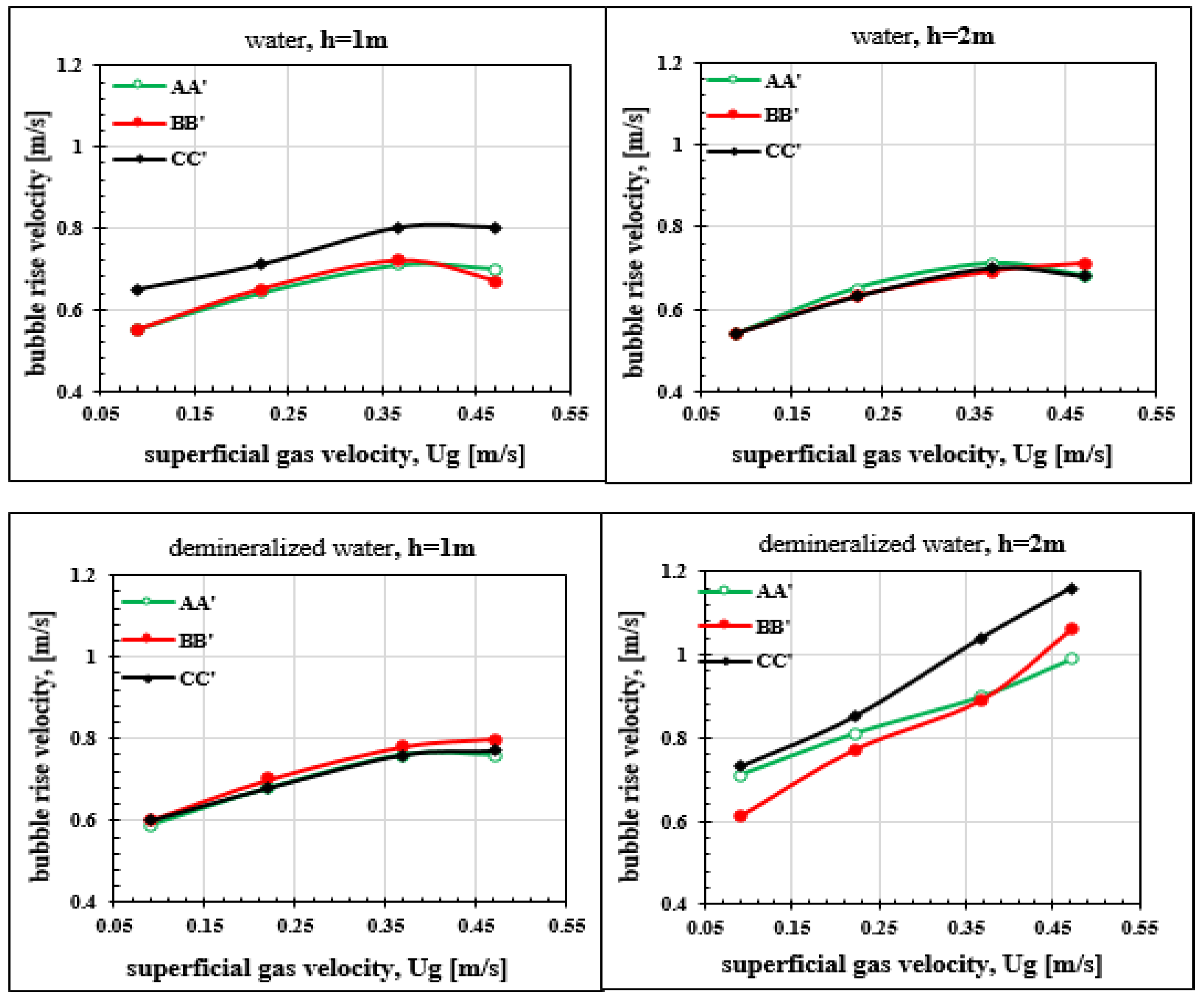
3.5.2. Bubble Rise Velocity

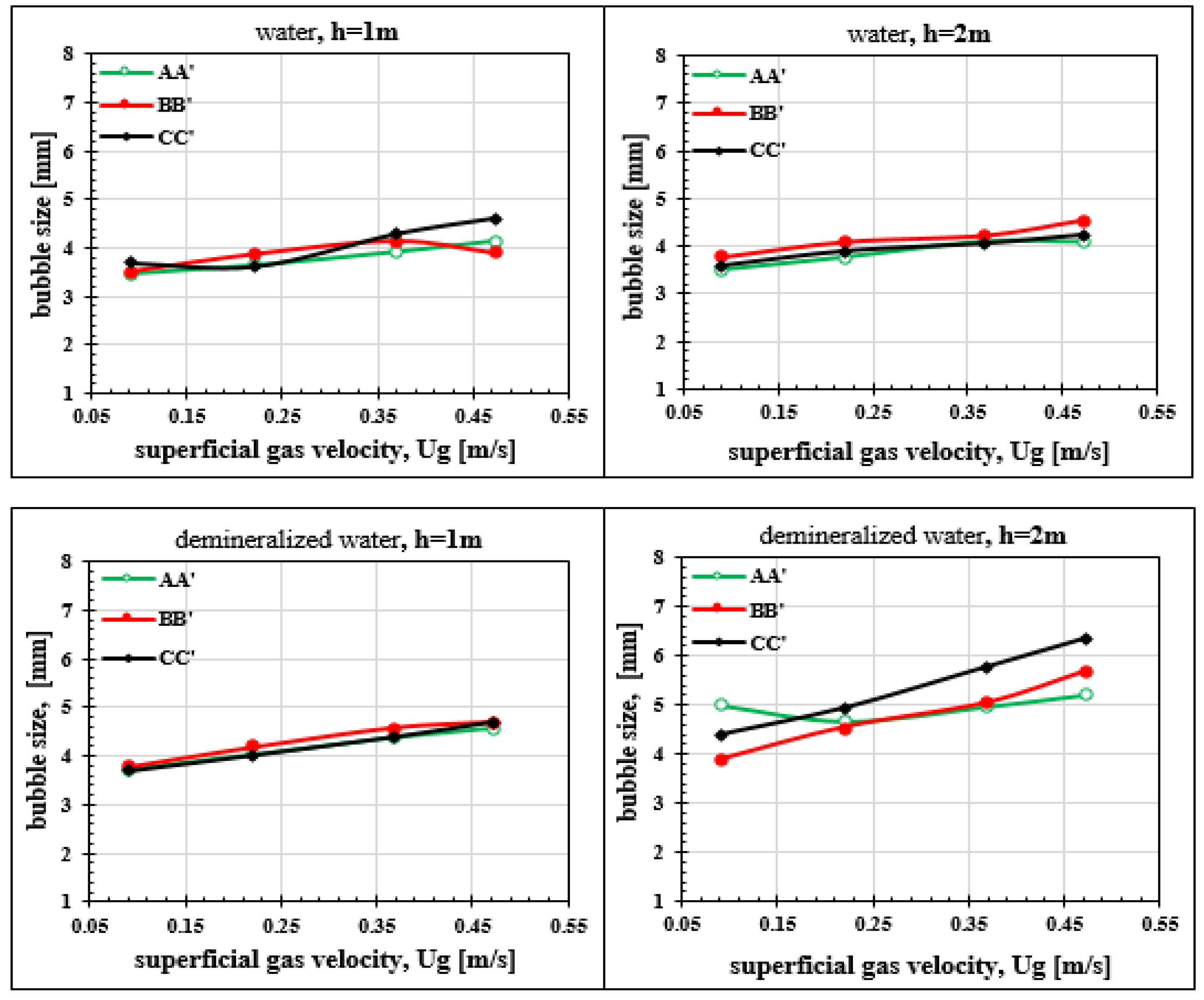
The bubble rise velocities measured with the optical bi-probe are averages made on a sample of ${10}^4$ bubbles. These measurements are made in ordinary water and demineralized water to evaluate the effect of water quality on the rate of rise of air bubbles. For each of these types of water, the measurements are also made on the two vertical measurement positions: 1 m and 2 m from the column base. The results of the bubble rise velocity measurements are presented as a function of according to the superficial gas velocity on Figure 18. For each measurement configuration, five air flows are tested: 10 L·min${}^{-1}$; 20 L·min${}^{-1}$; 30 L·min${}^{-1}$; 35 L·min${}^{-1}$ and 40 L·min${}^{-1}$. In order to observe the transverse gas velocity profile, measurements on the radial plane and along three diameters (AA’, BB’ and CC’) are also presented in the same figures. For all cases of velocity measurement, the radial gas velocity profile is homogeneous and the values obtained for the three diameters are very close. The bubble rise velocity increases until airflow of 35 L·min${}^{-1}$. Beyond this rate (35 L·min${}^{-1}$), a threshold effect is set up and the velocity no longer increases. As explained for $W_G$, this is due to the appearance of the counter air-lift causing a slowing of the flow velocity of the two-phase mixture. The effect of counter air-lift appears as soon as one reaches a superficial gas velocity of rise $U_G=0.36$ m·s${}^{-1}$ (Figure 9).

The quality of the water, as the hardness, has a significant effect on the bubble rise velocities which is greater in deionized water than in ordinary water. This difference is more pronounced at 2 m height: $U_G=0.75$ m·s${}^{-1}$ in ordinary water and $U_G=1.16$ m·s${}^{-1}$ in demineralized water, which gives a difference of 46% (Figure 19). These results are consistent with Clift et al. [38] who has reported that speed decreases when water is contaminated. Thus, the evolution towards an increase or a decrease of the coalescence, thus of the bubble velocity, will depend on the nature of impurities present in the water. Figure 19 below represents the real rise velocities of the bubbles obtained by global measurement and the bubble rise velocities obtained with the optical bi-probe. There is a large difference between these two velocities. The optical bi-probe seems to underestimate the bubble rise velocity rates of about $50\%$ [39]. To Besagni et al. [36] his underestimation is mainly due to the impact of the bubbles with the tips of the bi-probe. This impact induces a deformation of the morphology of the bubbles and leads to an over-estimation of the rise time of the bubbles. The increase in bubble rise time leads to an underestimation of the rate of rise obtained by the optical bi-probe. The relative difference reported in literature concerning the measurement of the bubble rise velocity using an optical bi-probe reaches up to 45% [19].

3.5.3. Bubble Size

Average bubble diameter is determined using the optical bi-probe. The results show that the bubble size distribution is uniform on the horizontal plane. The diameter of the bubbles increases linearly with the superficial gas velocity and, for all measurement axes, the profile remains practically the same even with a mean diameter of 4.17 mm (Figure 20). In ordinary water, the height position of the measuring point by the optical bi-probe does not seem to have a significant effect on the bubble size. On the other hand, in demineralised water, diameters are larger than in ordinary water. The diameters measured at 2 m height in demineralized water are larger than those obtained at 1 m. This difference in bubble size is explained by the fact that, in demineralized water, the coalescence of the bubbles is more significant during their rise. Measurements made in demineralized water at 2 m height indicate a great irregularity of the horizontal profile of the mean diameters of the bubbles.

4. Conclusions

The Hydrodynamic study presented in this paper is carried out on a bubble column under depression. The column studied consists of two vertical concentric tubes (inside diameter 0.08 m and 0.15 m) connected at a raceway. The objective of this study was to experimentally determine the phases characterization of an airlift under vacuum: gas holdup, bubble rise velocity and bubble size. These hydrodynamic parameters are studied using an optical bi-probe for local measurement and a differential pressure sensor for global characterization of gas holdup. Global measurement of gas holdup made it possible to determine the superficial gas velocity and thus to relate the global hydrodynamics of the system to the properties of the local flow. The measurements are made with tap and demineralized water in order to study the effect of water quality on the desired hydrodynamic parameters. The global analysis made it possible to demonstrate that beyond a superficial gas velocity $U_G=0.36$ m·s${}^{-1}$ a transition flow regime is observed, giving rise to a counter-airlift effect. This effect reduces the bubble rise velocity, liquid velocity and therefore the pumping capacity is limited. A clamping of the liquid flow does not seem to influence the appearance of the counter-airlift at the same limit superficial gas velocity and the pumping rate is always the same because the liquid velocity is linked in this airlift configuration at the superficial gas velocity. The analysis of the bubble rise velocity obtained with optical bi-probe shows that this velocity increases with gas holdup. Water quality seems to have a significant effect on it, the values with deionized water are higher than in tap water. It thus appears that the evolution towards an increase or a decrease of the coalescence, therefore of bubble rise velocity, will depend on the nature of impurities in the water. There is also an underestimation of bubble rise velocity by the optical bi-probe of about $50\%$. This is due to the fact that the probe tip hooks the bubble at the time of detection and induces a deformation of its morphology leading to an overestimation of the rise time. Results of various measurements indicate that the water quality does not seem to have an effect on gas holdup. Measurements made at two heights are very close, the measuring section height does not significantly influence the gas holdup. However, in demineralized water, a slight asymmetry of gas holdup is observed. Coalescence seems to have as much impact on sensor probe detection time as on bubble size, which would explain the limited increase in gas holdup with height. Bubble diameter increases linearly with gas holdup. It is larger in demineralized water than in tap water, which confirms the important influence of water quality earlier observed with the bubble rise velocity. Finally, this article contributes to the existing discussion on the hydrodynamics of bubble columns and is, to our knowledge, the first experimental study on hydrodynamic characterization of a bubble column under vacuum. Results obtained could be useful for an optimization study of airlift under depression.

References

1. Deen, N.G.; Mudde, R.F.; Kuipers, J.A.M.; Zehner, P.; Kraume, M. Bubble columns. In Ullmann’s Encyclopedia of Industrial Chemistry; Wiley-VCH Verlag: Weinheim, Germany, 2000. [Google Scholar]
2. Barrut, B. Etude et Optimisation du Fonctionnement d’une Colonne Airlift à Dépression: Application à L’aquaculture. Ph.D. Thesis, Université Montpellier, Montpellier, France, 2011. [Google Scholar]
3. Chaumat, H.; Billet-Duquenne, A.; Augier, F.; Mathieu, C.; Delmas, H. On the reliability of an optical fibre probe in bubble column under industrial relevant operating conditions. Exp. Therm. Fluid Sci. 2007, 31, 495–504. [Google Scholar] [CrossRef]
4. Rene, F.; Lemarie, G.; Champagne, J.Y.; Morel, R. Procédé et Installation de Traitement d’un Effluent Aqueux, en vue d’en Extraire au Moins un Composé Gazeux Dissous; Application à L’aquaculture en Milieu Aqueux Recirculé. FR0702308A, 29 March 2007. (In French). [Google Scholar]
5. Singh, B.K.; Quiyoom, A.; Buwa, V.V. Dynamics of gas–liquid flow in a cylindrical bubble column: Comparison of electrical resistance tomography and voidage probe measurements. Chem. Eng. Sci. 2017, 158, 124–139. [Google Scholar] [CrossRef]
6. Besagni, G.; Inzoli, F.; De Guido, G.; Pellegrini, L.A. The dual effect of viscosity on bubble column hydrodynamics. Chem. Eng. Sci. 2017, 158, 509–538. [Google Scholar] [CrossRef]
7. Azzopardi, B.; Zhao, D.; Yan, Y.; Morvan, H.; Mudde, R.; Lo, S. Hydrodynamics of Gas-Liquid Reactors: Normal Operation and Upset Conditions; John Wiley & Sons: Hoboken, NJ, USA, 2011. [Google Scholar]
8. Young, M.A.; Carbonell, R.G.; Ollis, D.F. Airlift bioreactors: Analysis of local two-phase hydrodynamics. AIChE J. 1991, 37, 403–428. [Google Scholar] [CrossRef]
9. Adetunji, O.; Rawatlal, R. Estimation of bubble column hydrodynamics: Image-based measurement method. Flow Meas. Instrum. 2017, 53, 4–17. [Google Scholar] [CrossRef]
10. Besbes, S.; El Hajem, M.; Aissia, H.B.; Champagne, J.Y.; Jay, J. PIV measurements and Eulerian–Lagrangian simulations of the unsteady gas–liquid flow in a needle sparger rectangular bubble column. Chem. Eng. Sci. 2015, 126, 560–572. [Google Scholar] [CrossRef]
11. Giovannettone, J.; Tsai, E.; Gulliver, J. Gas void ratio and bubble diameter inside a deep airlift reactor. Chem. Eng. J. 2009, 149, 301–310. [Google Scholar] [CrossRef]
12. Lau, Y.M.; Sujatha, K.T.; Gaeini, M.; Deen, N.G.; Kuipers, J.A.M. Experimental study of the bubble size distribution in a pseudo-2D bubble column. Chem. Eng. Sci. 2013, 98, 203–211. [Google Scholar] [CrossRef]
13. Chaouki, J.; Larachi, F.; Duduković, M.P. Noninvasive Tomographic and Velocimetric Monitoring of Multiphase Flows. Ind. Eng. Chem. Res. 1997, 36, 4476–4503. [Google Scholar] [CrossRef]
14. Cartellier, A. Optical probes for local void fraction measurements: Characterization of performance. Rev. Sci. Instrum. 1990, 61, 874–886. [Google Scholar] [CrossRef]
15. Galaup, J.P.; Delhaye, J.M. Utilisation de sondes optiques miniatures en écoulement diphasique gaz-liquide. Application à la mesure du taux de présence local et de la vitesse locale de la phase gazeuse. La Houille Blanche 1976, 1, 17–30. [Google Scholar] [CrossRef]
16. Hinata, S. A study on the measurement of the local void fraction by the optical fiber glass probe. Bull. JSME 1972, 15, 1228–1235. [Google Scholar] [CrossRef]
17. Danel, F.; Delhaye, J.M. Sonde optique pour mesure du taux de présence local en écoulement diphasique. Mes. Regul. Autom. 1971, 36, 99–101. [Google Scholar]
18. Miller, N.; Mitchie, R.E. The Development of a Universal Probe for Measurement of Local Voidage in Liquid-Gas Two-Phase Flow Systems; Atomic Power Constructions Ltd.: Heston, UK, 1969. [Google Scholar]
19. Cartellier, A.; Barrau, E. Monofiber optical probes for gas detection and gas velocity measurements: Conical probes. Int. J. Multiph. Flow 1998, 24, 1265–1294. [Google Scholar] [CrossRef]
20. Rojas, G.; Loewen, M.R. Fiber-optic probe measurements of void fraction and bubble size distributions beneath breaking waves. Exp. Fluids 2007, 43, 895–906. [Google Scholar] [CrossRef]
21. Yamada, M.; Saito, T. A newly developed photoelectric optical fiber probe for simultaneous measurements of a CO2 bubble chord length, velocity, and void fraction and the local CO2 concentration in the surrounding liquid. Flow Meas. Instrum. 2012, 27, 8–19. [Google Scholar] [CrossRef]
22. Pjontek, D.; Parisien, V.; Macchi, A. Bubble characteristics measured using a monofibre optical probe in a bubble column and freeboard region under high gas holdup conditions. Chem. Eng. Sci. 2014, 111, 153–169. [Google Scholar] [CrossRef]
23. Raimundo, P.M. Analysis and Modelization of Local Hydrodynamics in Bubble Columns. Ph.D. Thesis, Université Grenoble Alpes, Grenoble, France, 2015. [Google Scholar]
24. Besagni, G.; Brazzale, P.; Fiocca, A.; Inzoli, F. Estimation of bubble size distributions and shapes in two-phase bubble column using image analysis and optical probes. Flow Meas. Instrum. 2016, 52, 190–207. [Google Scholar] [CrossRef]
25. Aliyu, A.M.; Kim, Y.K.; Choi, S.H.; Ahn, J.H.; Kim, K.C. Development of a dual optical fiber probe for the hydrodynamic investigation of a horizontal annular drive gas/liquid ejector. Flow Meas. Instrum. 2017, 56, 45–55. [Google Scholar] [CrossRef]
26. Peytraud, J.F. Etude de la Tomographie Electrique Pour la Mesure du Taux de Vide Local en Ecoulements Diphasiques. Ph.D. Thesis, Grenoble INPG, Grenoble, France, 1995. [Google Scholar]
27. Serdula, C.D.; Loewen, M.R. Experiments investigating the use of fiber-optic probes for measuring bubble-size distributions. IEEE J. Ocean. Eng. 1998, 23, 385–399. [Google Scholar] [CrossRef]
28. Kiambi, S.L.; Duquenne, A.M.; Dupont, J.B.; Colin, C.; Risso, F.; Delmas, H. Measurements of Bubble Characteristics: Comparison Between Double Optical Probe and Imaging. Can. J. Chem. Eng. 2003, 81, 764–770. [Google Scholar] [CrossRef]
29. Vejražka, J.; Večeř, M.; Orvalho, S.; Sechet, P.; Ruzicka, M.C.; Cartellier, A. Measurement accuracy of a mono-fiber optical probe in a bubbly flow. Int. J. Multiph. Flow 2010, 36, 533–548. [Google Scholar] [CrossRef]
30. Mizushima, Y.; Sakamoto, A.; Saito, T. Measurement technique of bubble velocity and diameter in a bubble column via single-tip optical-fiber probing with judgment of the pierced position and angle. Chem. Eng. Sci. 2013, 100, 98–104. [Google Scholar] [CrossRef]
31. Clark, N.N.; Turton, R. Chord length distributions related to bubble size distributions in multiphase flows. Int. J. Multiph. Flow 1988, 14, 413–424. [Google Scholar] [CrossRef]
32. Liu, W.; Clark, N.N. Relationships between distributions of chord lengths and distributions of bubble sizes including their statistical parameters. Int. J. Multiph. Flow 1995, 21, 1073–1089. [Google Scholar] [CrossRef]
33. Simonnet, M. Étude Expérimentale du Mouvement de Bulles en Essaim: Application à la Simulation Numérique de Colonnes à Bulles. Ph.D. Thesis, Vandoeuvre-les-Nancy, INPL, Lorraine, France, 2005. [Google Scholar]
34. Colombet, D. Modélisation de Réacteurs Gaz-Liquide de Type Colonne à Bulles en Conditions Industrielles. Ph.D. Thesis, Toulouse, INSA, Toulouse, France, 2012. [Google Scholar]
35. Moujaes, S.; Dougall, R.S. Experimental investigation of cocurrent two-phase flow in a vertical rectangular channel. Can. J. Chem. Eng. 1987, 65, 705–715. [Google Scholar] [CrossRef]
36. Besagni, G.; Inzoli, F. Influence of internals on counter-current bubble column hydrodynamics: Holdup, flow regime transition and local flow properties. Chem. Eng. Sci. 2016, 145, 162–180. [Google Scholar] [CrossRef]
37. Wilkinson, P.M.; Spek, A.P.; van Dierendonck, L.L. Design parameters estimation for scale-up of high-pressure bubble columns. AIChE J. 1992, 38, 544–554. [Google Scholar] [CrossRef]
38. Clift, R.; Grace, J.; Weber, M. Bubbles, Drops, and Particles; Academic Press: New York, NY, USA, 1978. [Google Scholar]
39. Xue, J.; Al-Dahhan, M.; Dudukovic, M.P.; Mudde, R.F. Bubble Dynamics Measurements Using Four-Point Optical Probe. Can. J. Chem. Eng. 2003, 81, 375–381. [Google Scholar] [CrossRef]
Figure 1. Experimental setup.
Fluids 04 00080 g001
Figure 2. Convergence of gas holdup.
Fluids 04 00080 g002
Figure 3. Convergence of bubble size.
Fluids 04 00080 g003
Figure 4. Convergence of bubble rise velocity.
Fluids 04 00080 g004
Figure 5. Evolution of the liquid flow as a function of the air flow.
Fluids 04 00080 g005
Figure 6. Effect of the clamping of the liquid flow on the pumping regime.
Fluids 04 00080 g006
Figure 7. Relationship between theoretical liquid velocity ( U L ) and actual liquid velocity ( W L ).
Fluids 04 00080 g007
Figure 8. Schematic representation of the radial measurement axes by the optical bi-probe.
Fluids 04 00080 g008
Figure 9. Relationship between bubble rise velocity and superficial gas velocity.
Fluids 04 00080 g009
Figure 10. Relationship between actual liquid velocity and superficial gas velocity.
Fluids 04 00080 g010
Figure 11. Relationship between slip gas velocity and superficial gas velocity.
Fluids 04 00080 g011
Figure 12. Relationship between global gas holdup and volumetric air flow.
Fluids 04 00080 g012
Figure 13. Relationship between local gas holdup and global gas velocity.
Fluids 04 00080 g013
Figure 14. Relationship between local and global gas holdup.
Fluids 04 00080 g014
Figure 15. Radial distribution of gas holdup for different traverses.
Fluids 04 00080 g015
Figure 16. Evolution of radial distribution of gas holdup with air flow.
Fluids 04 00080 g016
Figure 17. Relationship between global and local gas holdup with superficial gas velocity.
Fluids 04 00080 g017
Figure 18. Relationship between bubble rise velocity and superficial gas velocity.
Fluids 04 00080 g018
Figure 19. Relationship between bubble rise velocity ( U G L and W G ) and superficial gas velocity ( U G ).
Fluids 04 00080 g019
Figure 20. Relationship between bubble size and superficial gas velocity.
Fluids 04 00080 g020