Meshless Modeling of Flow Dispersion and Progressive Piping in Poroelastic Levees ^†

Abstract

Performance data on earth dams and levees continue to indicate that piping is one of the major causes of failure. Current criteria for prevention of piping in earth dams and levees have remained largely empirical. This paper aims at developing a mechanistic understanding of the conditions necessary to prevent piping and to enhance the likelihood of self-healing of cracks in levees subjected to hydrodynamic loading from astronomical and meteorological (including hurricane storm surge-induced) forces. Systematic experimental investigations are performed to evaluate erosion in finite-length cracks as a result of transient hydrodynamic loading. Here, a novel application of the localized collocation meshless method (LCMM) to the hydrodynamic and poroelastic problem is introduced to arrive at high-fidelity field solutions. Results from the LCMM numerical simulations are designed to be used as an input, along with the soil and erosion parameters obtained experimentally, to characterize progressive piping.

1. Introduction

Water retaining structures, such as dams, canals, and levees, are essential for managing water resources. Often, the most economical, environmentally-conscious, and sustainable construction methods require construction using locally available soils. At times, it can be possible to construct these structures economically with masonry, concrete, and alternative materials. However, it is necessary that these structures be placed on high-quality foundation soils for satisfactory performance in the event that a solid rock stratum is not available at a reasonable depth. Therefore, the safety of these hydraulic structures depends on the capacity of the soils in the body and/or the foundation of the structure to resist the seepage forces generated by the retained water. That is, the soils should be able to safely allow the flow of retained without sustaining structural damage or erosion of soils.

Often times, the seepage on the downstream sides of hydraulic structures is found to be laden with soil particles, commonly referred to as “sand boils.” Excessive seepage at specific points on the downstream side is indicative of preferential flow that may be due to anomalies in construction, foundation strata, or may indicate the formation of internal cracks voids due to movement of soils under seepage forces. Formation and gradual expansion of internal voids is frequently referred to as “progressive piping.” This phenomenon may proceed unnoticed as this phenomenon occurs deep within the structure. These internal voids may collapse and form surface sinkholes, and in some cases may rapidly cause breaching failure of the structure. ICOLD [1] and Foster et al. [2] conducted statistical analyses of dam failures and found that internal soil erosion is a predominant cause of failure. Furthermore, Zaslavsky and Kassiff [3], Vallejo [4], and Kakuturu and Reddi [5] have described the conditions that promote progressive piping and outlined some basic methods for their assessment.

The success of any numerical method depends on the input of appropriate material characteristics and the experimental methods that are adopted for obtaining those characteristics. In our numerical approach, we consider the levee soil as an isotropic poroelastic material, neglecting the effects of internal particle movement. Therefore, a set of three unique values of the hydraulic conductivity, elastic modulus, and Poisson’s ratio are used for calculating the pore pressures and internal stresses around a typical crack in a levee. It should be pointed here that the levee soils exhibit much higher hydraulic conductivity in the two horizontal directions compared to the vertical direction, because of the rolling compaction of the soil in horizontal layers during construction. The stresses experienced by the levee soils are usually much smaller compared to the stresses experienced by foundation soils for which a lot of data is available in the literature. Most relevant stress–strain characteristics for soils can be obtained by conducting tri-axial shear tests, which; however, produce non-linear curves with initial portions being unreliable due to experimental and equipment limitations. Therefore, it is customary to take either a tangent modulus or secant modulus for the desirable range of stresses. The triaxial sear test also facilitates measurement of volume change for reliable estimation of the Poisson’s ratio.

1.1. Background

The first reservoir filling is considered very crucial to the integrity of the structure, as desiccation cracks may develop between reservoir construction and reservoir filling, and the filling may result in stresses that enlarge these cracks. A similar seepage failure mechanism is reported by Zhang and Chen [6], whereby catastrophic failure occurred in the first reservoir filling of a 71 m high Chinese rockfill dam. Additionally, cracks may develop during the service life of the structure, especially during intermittent dry periods, when foundation compression or even minor earthquakes may result in differential settlement of structural components. In laboratory-controlled conditions, Lakshmikantha et al. [7] employed image analysis techniques on clay-like soils to develop predictive models for the development of desiccation cracks and understand the conditions that influence cracking.

There are several documented instances of major piping-induced failures of water retaining structures, such as that of the Teton Dam as reported by Watts et al. [8], the Chagrin River Dam in Ohio described by Evans et al. [9], among several other cases reported by ICOLD (1995) [1]. Frequent problems faced by levees along the Mississippi, Red and Sacramento rivers. In the light of the Katrina disaster in Louisiana, public concerns have been heightened over frequent levee problems along the Mississippi, Sacramento, and Red rivers. These levee problems have been documented in several instances. Mansur et al. [10] reported the presence of sand boils caused by piping along the Mississippi river. Sills et al. [11] inferred that piping was the probable reason for failure of some levees in New Orleans that were not overtopped during the Katrina hurricane. Hagerty [12,13] provides a comprehensive and visual description of conditions that result in piping and methods for identifying piping erosion amid the complex mechanisms and interactions involved in emergent seepage failures. Gattinoni and Francani [14] analyzed the evolution of piping phenomenon and developed a model for studying the slope instability triggered by piping to understand failure conditions and applied it to the 1985 Stava Valley disaster that took place in Italy.

Internal erosion and progressive piping were detected in several experimental and in situ investigations of problem-riddled levees and dams. Through exhuming operations that confirmed piping, Johansen and Eikevik [15] described the internal erosion suffered by the Jukla Dams in Norway and the rehabilitation measures implemented. Studies by Chen et al. [16], Sjödahl [17], Inazaki [18], Rucker et al. [19], and Hung et al. [20] relied upon non-invasive geophysical methods that provided qualitative evidence of progressive piping in water retaining structures. Williams [21], Holden [22], Wang and Chen [23], and Lee et al. [24] made use of chemical or temperature tracers in combination with other methods for detection of progressive piping.

Though thousands of small cracks may develop in a hydraulic structure over the course of a year, most of these will self-heal with only a very few having a likelihood of growing larger and eroding to form the progressive piping conditions that result in failure. Some of the studies for developing a mechanistic understanding of progressive piping are by Sellmeijer and Koenders [25], Ojha et al. [26,27], Kakuturu and Reddi [5], Bonelli et al. [28], El Shamy and Aydin [29], and Bonelli and Brivois [30]. Recent research investigations by Fell et al. [31], Ojkan [32], and Yi [33] have focused on the transience and evolution of progressive piping due to natural conditions. Experimental methods are described by Kakuturu and Reddi [34] for the evaluation and characterization of some soil properties that influence progressive piping and, conversely, self-healing of cracks in earth dams.

Thus, it can be summarized that the mechanics of both fluidic and solid stratum field variables such as pore water pressures, hydraulic gradients, and principal stresses in the region surrounding the tiny cracks are the prime external drivers of crack expansion, erosion and progressive piping. These factors in conjunction with soil properties, shear strength, compressibility, gradation, interlocking, particle transportability, pore water chemistry, etc., govern the fate of tiny cracks.

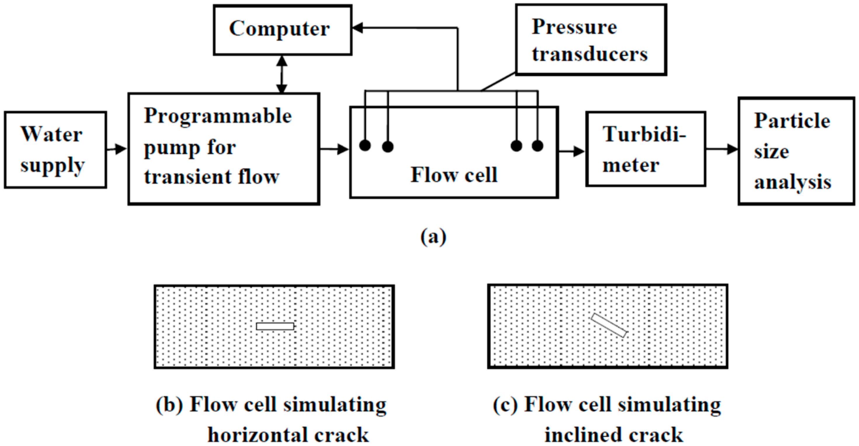
1.2. Experimental Investigations of Progressive Piping

The objective of experimentation is to empirically quantify the progressive piping of cracks in soil samples, namely by applying a transient force system that represents typical hurricane forces in levees [34]. The forces in this system were estimated by considering the relevant surface water hydrodynamics on the levees. Laboratory experiments were conducted on soils that typically form the body and foundation of levees. In addition to observing piping, the experiment focused on obtaining soil properties needed for the development of the mathematical model.

A design of the experimental setup is shown in Figure 1. One of the important components of this experimental setup was the computer programmable pump that created a chosen transient force system. The flow cell housed a soil sample with pre-formed cracks of given dimensions in chosen orientations. Two simple experimental features successfully implemented were: (1) Pressure transducers in and outside the flow cell to minute pressures as the initial cracks grow into large pipes, and (2) particle size analyses of effluent to observe the mass concentration and size of eroded particles.

Another objective of experimentation is to evaluate the soil properties required for numerical implementation of the mathematical model of progressive piping. The soil properties that are characterized are: (1) Critical hydraulic gradient that must be exceeded for particle dislodgment in the upstream part of the crack, (2) rate of particle dislodgement once the actual hydraulic gradient exceeds the critical value, (3) critical shear stress that must be exceeded for surface erosion on the walls of the crack, (4) rate of the surface erosion once the actual shear stress exceeds that critical value, (5) parameters influencing the hydraulic fracturing, and (6) particle entrapment parameter of soil downstream of the crack. Example designs of the flow cells for obtaining these parameters are shown as Figure 2.

The results of aforementioned experimentation were used in defining parameters implemented in the numerical modeling techniques employed here.

1.3. Numerical Modeling

While conventional modeling techniques, such as the finite element methods (FEM) and finite volume methods (FVM) have been developed and routinely implemented to model complex multi-physics problems, they both require significant effort in mesh generation. The term “meshless methods” refers to a class of numerical techniques that typically rely on either a global or localized interpolation on non-ordered spatial point distributions, as opposed to a connected mesh that discretizes the domain of interest. Given the independence of an ordered mesh, there has been much interest in the development of meshless techniques, which are a relative newcomer to field of numerical methods, as they offer the hope of reducing the effort devoted to model preparation [35,36,37,38,39,40,41]. The meshless approach finds its origin in classical spectral or pseudo-spectral methods [42,43,44,45,46], which are based on global orthogonal functions such as Chebyshev or Legendre polynomials. However, these methods require a regular nodal point distribution for the implementation of orthogonal polynomials. This is contrasted with meshless methods which use a nodal or point distribution that is not required to be uniform or regular without loss of accuracy in field representation, due to the fact that most meshless techniques rely on global radial-basis functions (RBF) [47,48,49,50,51,52,53,54,55,56,57]. However, global RBF interpolation poses several issues and so, localized collocation meshless methods [58,59,60] have recently been proposed to address many of these issues.

In a series of recent publications [61,62,63,64,65,66,67,68,69,70], the co-authors have developed and validated a localized collocation meshless method (LCMM) based on the radial-basis function (RBF) interpolation for modeling of coupled viscous fluid flow, heat transfer problems, and fluid–structure interaction problems. The LCMM is shown to be computationally more efficient than a comparative finite volume method (FVM) [66,67] code whilst solving the partial differential conservation field equations of fluid flow and heat transfer on a non-ordered set of points. The method has been validated and verified against benchmark problems consisting of conventional finite volume codes for several cases, including lid-driven cavity flow, flow over a cylinder, the backward-facing step problem, and others [61,62,63,64,65,66,67,68,69,70].

2. Materials and Methods

2.1. Mathematical Model and Governing Equations

The equations that govern the flow of a fluid through a poroelastic medium are the Navier equation coupled with the Richards equations [71,72] as:

$$\begin{array}{c}G{\nabla }^2\overrightarrow{u}+\frac{G}{\left(1-2\nu \right)}\nabla \left(\nabla \cdot \overrightarrow{u}\right)=\nabla p\hfill \\ \varphi {\beta }_f\frac{\partial p}{\partial t}=\nabla \cdot \left[\frac{\kappa }{{\mu }_f}\left(\nabla p+{\rho }_f\overrightarrow{g}\right)\right]-\frac{\partial }{\partial t}\left(\nabla \cdot \overrightarrow{u}\right)\hfill \end{array}$$

(1)

Here, $p$ is the pore pressure, $\varphi$ is the porosity of the medium, $\kappa$ is the permeability of the medium, and ${\beta }_f, {\rho }_f, {\mu }_f$ are respectively the compressibility, density, and viscosity of the fluid flowing through the porous medium.

The Navier and Richards governing equations in (1) are strongly coupled (two-way) given the derivative operators on the field variables defined by both equations; the pore pressure appears on the right-hand side of the Navier equation, while the deformation field dilatation, $(\nabla \cdot \overrightarrow{u})$, appears on the right-hand side of the Richards equation.

The hydraulic conductivity, which indicates the relative permeability of the porous media to flow, is defined as:

$$K_h=\frac{\kappa {\rho }_f\left|\overrightarrow{g}\right|}{{\mu }_f}$$

(2)

The Darcy velocity of the flow through the porous medium is defined as:

$$\overrightarrow{V}=-\frac{\kappa }{{\mu }_f}\left(\nabla p+{\rho }_f\overrightarrow{g}\right)$$

(3)

Therefore, the actual front velocity of the flow is given by:

$${\overrightarrow{V}}_f=\frac{\partial \overrightarrow{u}}{\partial t}-\frac{\kappa }{\varphi {\mu }_f}\left(\nabla p+{\rho }_f\overrightarrow{g}\right)$$

(4)

The front velocity of the flow, ${\overrightarrow{V}}_f$, is used to track the location of the saturation time within the porous medium by adopting a volume-of-fluids (VOF) approach [73] as in two-phase flows. Thus, the location of the saturation (phreatic) line, $s$, at any time-level can be traced by a transport equation as:

$$\frac{\partial s}{\partial t}+\left({\overrightarrow{V}}_f\cdot \nabla \right)s=0$$

(5)

Thus, the VOF parameter, $s$, which indicates the saturation of the porous media by the fluid can be used to weight the value of the mechanical properties between the saturated and unsaturated values as:

$$G=\left(1-s\right)G^u+s{G}^s$$

(6)

Where, for instance, $G^u$, is the shear modulus of the unsaturated medium while $G^s$ is the shear modulus of the saturated medium.

Returning to the equations in (1), notice that the Navier equation is assumed to have reached steady-state while the Richards equation is assumed to be transient to account for porous media compressibility effects. These can be addressed by explicitly evolving the Richards equation in time using a first-order (Euler) time-derivative approximation, where:

$$p^{k+1}=p^k+\frac{\mathsf{\Delta }t}{\varphi {\beta }_f}\left\{\nabla \cdot \left[\frac{\kappa }{{\mu }_f}\left(\nabla p^k+{\rho }_f\overrightarrow{g}\right)\right]-\frac{\partial }{\partial t}\left(\nabla \cdot {\overrightarrow{u}}^k\right)\right\}$$

(7)

while updating the deformation field, $\overrightarrow{u}$, quasi-statically according to the Navier equation. Additionally, it is not necessary that the deformation field, $\overrightarrow{u}$, be updated at every time-level but rather every few time-levels, allowing one to accelerate the solution process. A simple systematic approach is adopted to determine when the deformation field needs to be updated based on quantified changes of such field.

Furthermore, it is important to note the difference in the time scale between which the pressure signal, $p$, propagates throughout the medium and the time scale at which the saturation front, $s$, moves within the medium. The difference is most easily observed in Equation (7), above, where the fluid compressibility, ${\beta }_f$, appears in the denominator of the right-hand side. Given the relative incompressibility of the fluid, ${\beta }_f$ is usually very small, which renders the propagation of the pressure signal, $p$, very fast when compared to the fluid velocity, ${\overrightarrow{V}}_f$, at which the saturation line, $s$, moves. Thus, special attention must be given when progressing Equations (5) and (7) as different time-steps, $\mathsf{\Delta }t$, will be implemented to advance the equations.

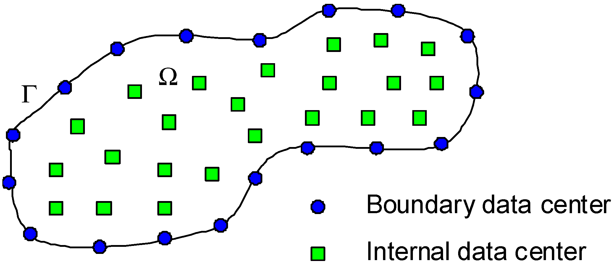
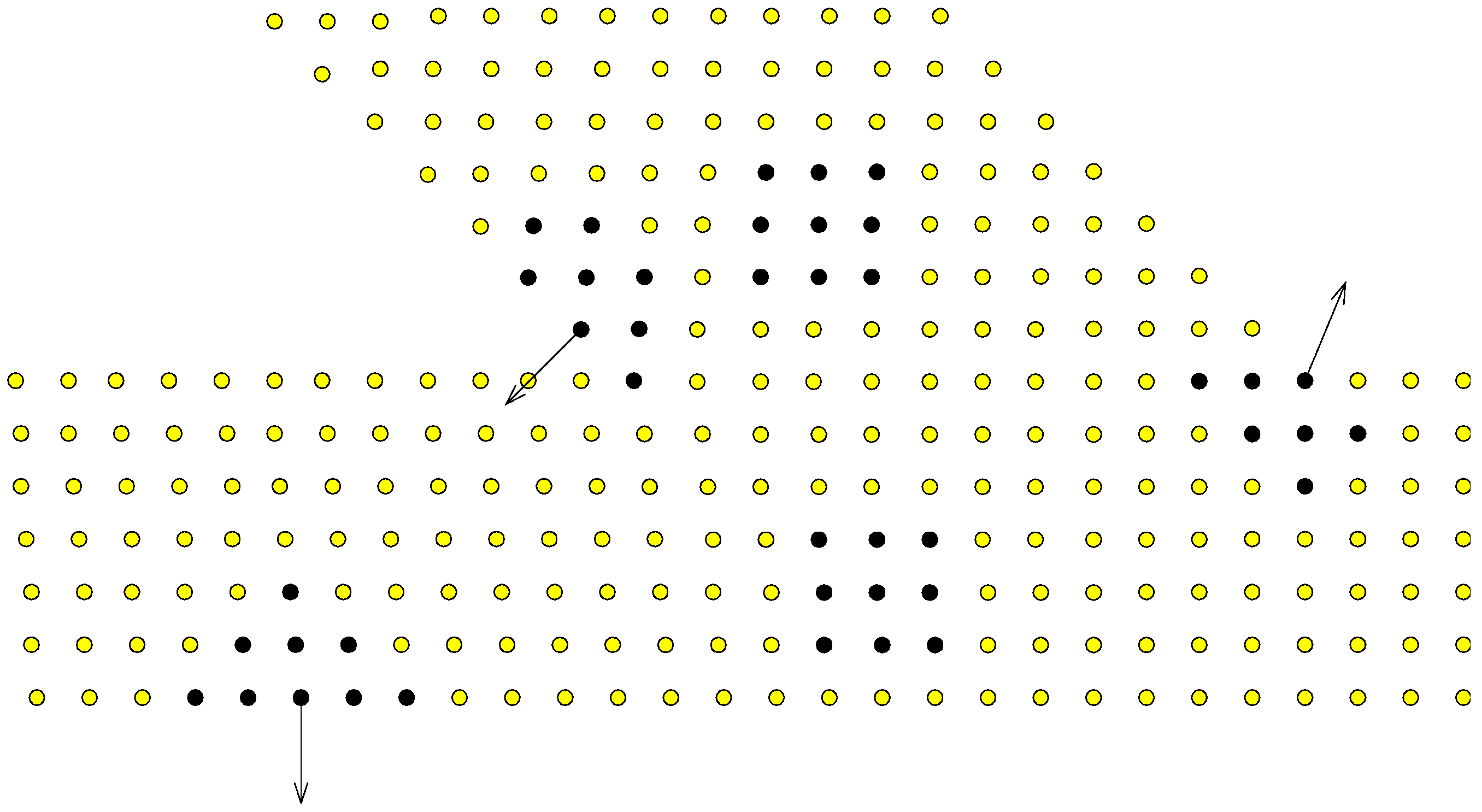
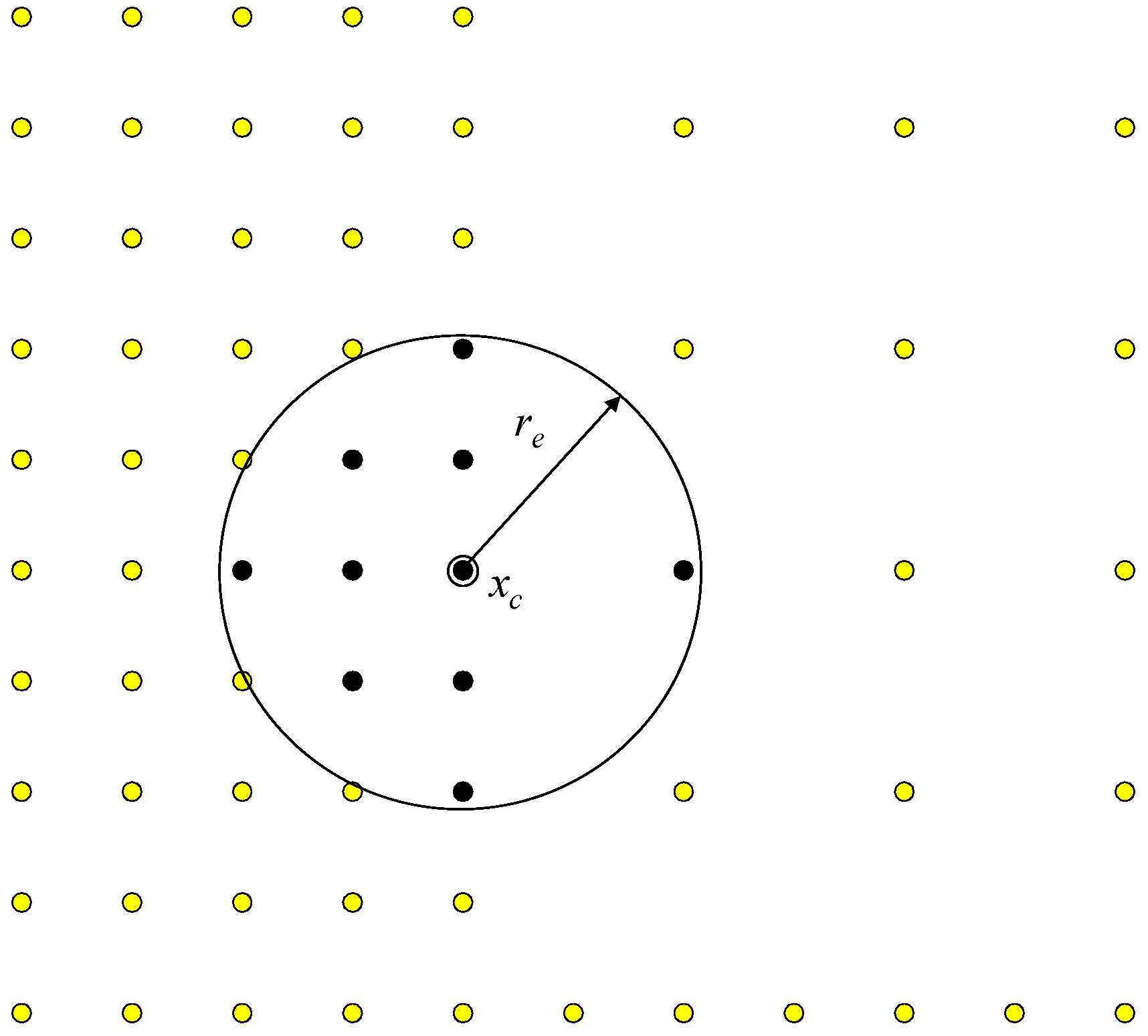
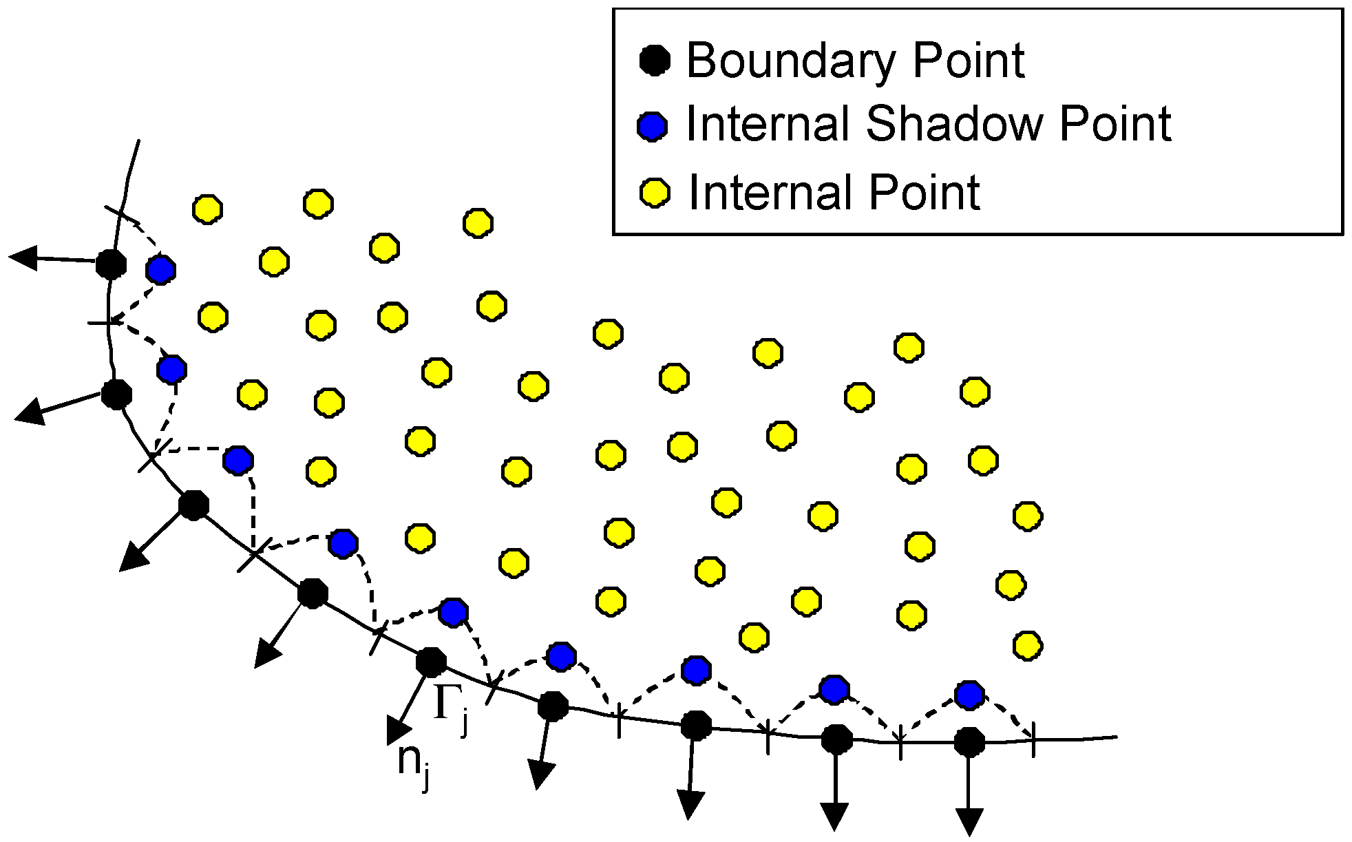
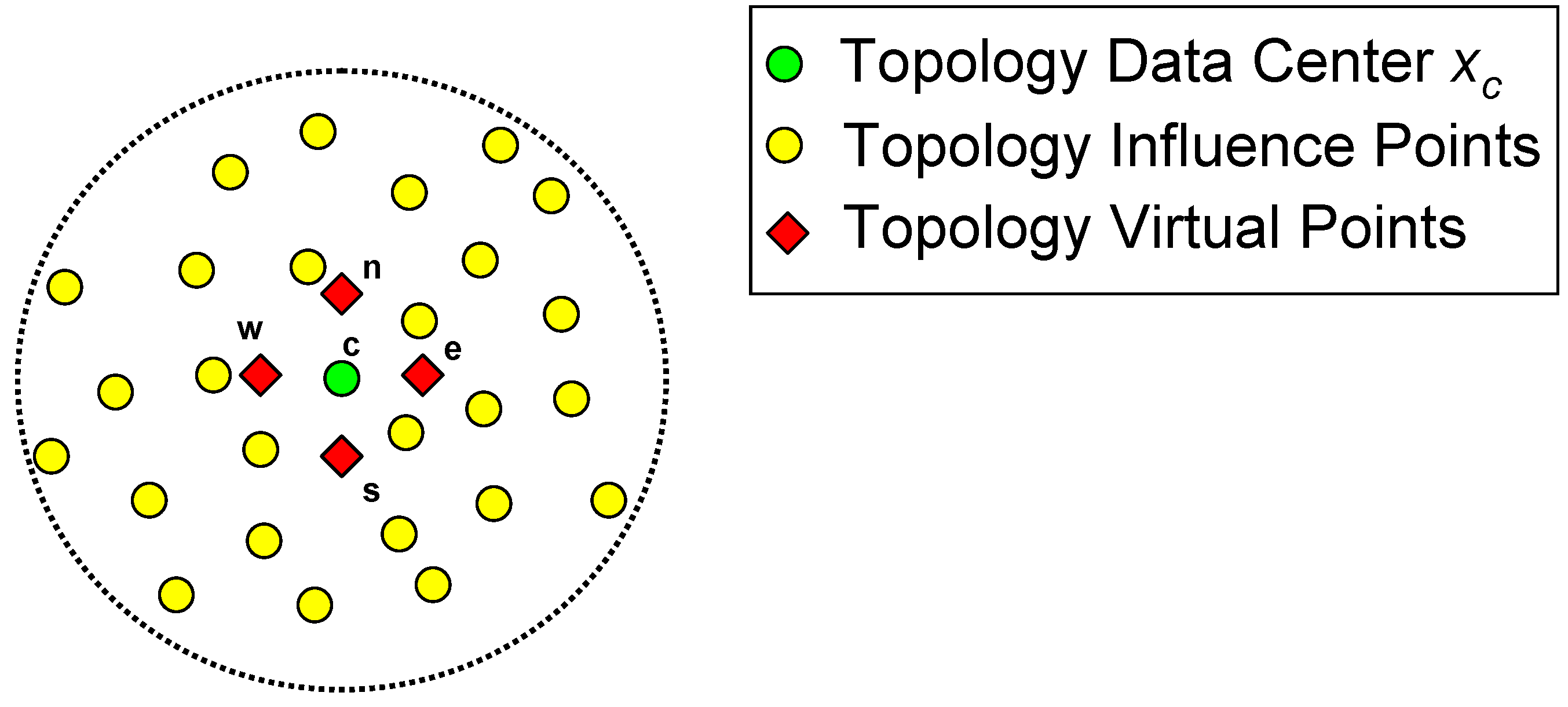
2.2. Localized Collocation Meshless Method Formulation

The meshless formulation begins by defining a domain, Ω, which is circumscribed by boundary, Γ, as depicted in Figure 3. A finite set of data centers, NC, are defined and is comprised of NB points on the boundary, and NI interior points within the domain. All the NC data centers will serve as collocation points for the localized expansion of the field variables in the domain. The only difference between boundary data centers and internal data centers is simply that boundary conditions are applied to the former while governing equations are applied to the latter.

To illustrate the meshless formulation, the diffusion for a general field variable, $\varphi$, in a generalized coordinate system, $x$, time, $t$, and a general diffusion coefficient, $\kappa$, will be taken into consideration as the governing equation valid in the domain, $\mathsf{\Omega }$, as:

$$\frac{\partial \varphi }{\partial t}\left(x,t\right)=\kappa {\nabla }^2\varphi \left(x,t\right)$$

(8)

In addition, a set of generalized boundary conditions for the variable, $\varphi$, on the boundary, $\mathsf{\Gamma }$, are given by:

$${\widehat{\beta }}_1\frac{\partial \varphi }{\partial n}+{\widehat{\beta }}_2\varphi ={\widehat{\beta }}_3$$

(9)

where ${\widehat{\beta }}_1, {\widehat{\beta }}_2,\mathrm{and}{\widehat{\beta }}_3$ are imposed coefficients of $\left(x,t\right)$ that dictate the boundary condition type and constrain values.

A linear localized expansion of a group or topology of influence points, NF, around each data center is sought such that:

$$\varphi \left(x\right)={\displaystyle \sum }_{j=1}^{NF}{\alpha }_j{\chi }_j\left(x\right)+{\displaystyle \sum }_{j=1}^{NP}{\alpha }_{j + NF}{P}_j\left(x\right)$$

(10)

The terms ${\alpha }_j$ represent unknown expansion coefficients, while the terms ${\chi }_j\left(x\right)$ are expansion functions defined a priori. At each time level, a different expansion will be performed; therefore, the expansion coefficients, ${\alpha }_j$, will vary as time progresses.

The expansion functions, ${\chi }_j\left(x\right)$, are selected from the family of radial-basis functions (RBF), particularly the inverse multiquadrics RBF. The family of RBF consist of algebraic expressions uniquely defined in terms of the Euclidean distance, $r_j\left(x\right)$, from a general field point, $x$, to an expansion point, $x_j$. Examples of these functions include the polyharmonics RBF, multiquadrics RBF, and gaussian RBF. For the examples presented in this paper, the multiquadrics RBF with $\left(n=1\right)$ is chosen as the expansion function and is given such that:

Multiquadrics RBF:

$${\chi }_j\left(x\right)={\left[r_j^2\left(x\right)+c^2\right]}^{n-\frac{3}{2}}$$

(11)

where $n$ is a positive exponent parameter and $c$ is a shape parameter. The effects of these parameters on the interpolation will be discussed later. In all cases, the radial distance, $r_j\left(x\right)$, is defined in the Cartesian coordinate system as:

$$r_j\left(x\right)=\sqrt{{(x-x_j)}^2+{(y-y_j)}^2},\hspace{1em}\hspace{1em}\hspace{1em}in 2D$$

(12)

To ensure that the general field variable approximation can capture constant and linear fields exactly, the interpolation functions are modified by NP additional polynomial functions, $P_j\left(x\right)$.

To reiterate, the globally collocated RBF-based meshless methods have some drawbacks, including poor conditioning of the ensuing algebraic set of equations. This can be addressed to some extent by domain decomposition and appropriate pre-conditioning [60]. Although very promising, these techniques can also be computationally intensive. A localized expansion approach [61,62,63,64,65,66,67,68,69,70,71,72,73] reduces the burden of the more common global interpolation methods [55,56,57,58,59,60] by limiting the field variable expansion over a smaller local topology around each data center, as opposed to the entire domain, to obtain field derivatives which are then implemented in time-marching or iterative numerical schemes. This yields multiple small interpolation matrices, which are significantly more manageable than the fully-populated global interpolation matrix of standard global. Since the approach relies on expanding known values of the field variables, it is only applicable if an explicit time-marching scheme with known initial conditions or an iterative solution scheme is formulated and is inapplicable directly to steady problems. However, this is not a drawback, as time marching can always be framed as a relaxation scheme for the iterative solution of steady-state problems. Thus, the selection of an influence region or localized topology of expansion around each data center is necessary for an accurate and unencumbered solution of the expansion and is easily accomplished by a circular search around each data center. For internal topologies, the search is automated to guarantee two conditions; first, that a minimum number of points will be included in the local topology and, second, that enough points are included in all directions around the internal data centers. For the topologies existing at domain boundaries, the search must also guarantee that points on opposing boundaries or points around a re-entry corner are not included within the topology. Figure 4 shows typical collocation topologies for internal and boundary data centers describing re-entry corners and opposing boundaries. Figure 5 shows an example of the circular search to build the topology around an internal data center of a non-uniform point distribution.

The collocation of the known field variable, f, (from previous time level or iteration step) at the points within the localized topology, leads to the following in matrix-vector form:

$$\left\{\varphi \right\}=\left[C\right]\left\{\alpha \right\}$$

(13)

Therefore, the expansion coefficients can be determined as:

$$\left\{\alpha \right\}={[C]}^{-1}\left\{\varphi \right\}$$

(14)

where the resulting collocation matrix is given by:

$$[C]={\left[\begin{array}{cccc}\begin{array}{c}{\chi }_1(x_1)\\ ⋮\end{array}& \begin{array}{c}\cdots \\ \ddots \end{array}& \begin{array}{c}{\chi }_{NF}(x_1)\\ ⋮\end{array}& \begin{array}{c}{P}_1(x_1)\\ ⋮\end{array}\\ {\chi }_1(x_{NF})& \cdots & {\chi }_{NF}(x_{NF})& P_1(x_{NF})\\ P_1(x_1)& \cdots & P_1(x_{NF})& 0\\ \begin{array}{c}\cdots \\ P_{NP}(x_1)\end{array}& \begin{array}{c}\ddots \\ \cdots \end{array}& \begin{array}{c}\cdots \\ P_{NF}(x_{NF})\end{array}& \begin{array}{c}⋮\\ 0\end{array}\end{array}\begin{array}{c}\begin{array}{c}\cdots \\ \ddots \end{array}\\ \cdots \\ \cdots \\ \begin{array}{c}\ddots \\ \cdots \end{array}\end{array}\begin{array}{c}\begin{array}{c}{P}_{NF}(x_1)\\ ⋮\end{array}\\ P_{NF}(x_{NF})\\ 0\\ \begin{array}{c}⋮\\ 0\end{array}\end{array}\right]}_{NF+NP,NF+NP}$$

(15)

And the right-hand side known vector is augmented as:

$$\left\{\varphi \right\}={\left\{\begin{array}{c}\varphi \left(x_1\right)\\ ⋮\\ \varphi \left(x_{NF}\right)\\ 0\\ ⋮\\ 0\end{array}\right\}}_{NF+NP,1}$$

(16)

To reiterate, the NF expansion functions, ${\chi }_j\left(x\right)$, are written in terms of the inverse multiquadrics RBF defined in Equation (11). Initially, c is determined for each expansion over the different localized topologies that span the domain based on (1) the average distance between data centers within the topology and (2) the total number of points within the topology. Then, an optimization routine is employed to modify the value of the shape parameter until the resulting collocation matrix, $\left[C\right]$, yields a condition number in the range between ${10}^{11}$ and ${10}^{12}$ (in double-precision), which has been documented to produce smooth derivative fields over the domain for a wide range of test functions.

It is important to mention that the collocation matrix, $\left[C\right]$, is dependent only on the geometrical point distribution within the localized topology. Thus, the optimization of the shape parameter, c, can be done at a setup stage when the topologies are assembled and prior to the actual solution process. However, there may be instances when optimization of the shape parameter, c, may be necessary at each solution time level, for example, when adaptive refinement is performed or when sharp discontinuities in the solution field are found.

The real advantage of the localized collocation approach is found in the calculation of derivatives of the field variable at the data center, $x_c$, of each topology. For instance, any linear differential operator, $L$, can be applied over the localized expansion equation as:

$$L\varphi \left(x_c\right)={\displaystyle \sum }_{j=1}^{NF}{\alpha }_{j}L{\chi }_j\left(x_c\right)+{\displaystyle \sum }_{j=1}^{NP}{\alpha }_{j + NF}L{P}_j\left(x_c\right)$$

(17)

This can be written in matrix-vector form, allowing the evaluation of the field variable derivatives at each of the data centers, $x_c$, to be found by a simple inner product of two small vectors: $\left\{L\right\}$ which can be pre-built and stored and $\left\{\varphi \right\}$ which is the updated field variable distribution in the topology of the data center. The derivation of the vector, $\left\{L\right\}$, is given in the Appendix A in Equations (A1)–(A5).

To illustrate this approach, the generalized diffusion equation, Equation (8), will be marched explicitly in time at each data center, $x_c$, using a first-order finite-differencing approximation as:

$${\varphi }_c^{k+1}={\varphi }_c^k+\kappa \mathsf{\Delta }t\left({\nabla }^2{\varphi }_c^k\right)$$

(18)

where the superscript, $k$, denotes the time level and $\mathsf{\Delta }t$ denotes the size of the time step. The Laplace operator on the right-hand side can be replaced by the localized RBF interpolation as:

$${\varphi }_c^{k+1}={\varphi }_c^k+\kappa \mathsf{\Delta }t{\left\{L\right\}}^T{\left\{\varphi \right\}}^k$$

(19)

Thus, the value of the solution field, $\left\{\varphi \right\}$, at every data center, $x_c$, at the next time level, k + 1, can be calculated from the solution field at the current time level, k, beginning with the initial field condition. This is done very efficiently, requiring only the current field solution and a simple inner product of the linear derivative operator.

The ability to estimate the field variables and their derivatives by simple inner products of pre-built vectors is precisely what makes the LCMM an attractive solution method. Notice that while the expansion coefficients need to be rebuilt at each time level, the multiquadrics RBF only need to be evaluated at the setup stage, when these vectors are being built. This provides tremendous computational advantages over global methods. First, this reduces the CPU burden of evaluating fractional powers and complicated functions at every level of a time-marching or iterative scheme. Additionally, without the need to allocate a global collocation matrix, using only very small vectors for each data center, the memory demands of this approach are minimal.

Furthermore, imposition of the generalized boundary conditions in Equation (9), at the boundary data centers, $x_c$, can be accomplished in a similar fashion. Recalling the general boundary condition from Equation (9) and replacing the normal derivative, $\partial /\partial n$, at the data center, $x_c$, with a localized expansion, yields:

$${\widehat{\beta }}_1{\{\partial n\}}^T\left\{\varphi \right\}+{\widehat{\beta }}_2{\varphi }_c={\widehat{\beta }}_3$$

(20)

where the interpolation vector, $\left\{\partial n\right\}$, yields the normal derivative of the field variable, $\left\{\varphi \right\}$, at the boundary topology data center, $x_c$. Ultimately, through some algebraic manipulation of the expression in Equation (20), a simple relation can be arrived at to determine the boundary field variable at the current time level, $k+1$, as:

$${\varphi }_c^{k+1}={\left\{\Gamma \right\}}^T{\left\{\varphi \right\}}^k$$

(21)

where the boundary interpolation vector, $\left\{\Gamma \right\}$, is composed by a combination of the normal derivative interpolation vector, $\left\{\partial n\right\}$, and the boundary condition coefficients, ${\widehat{\beta }}_1,{\widehat{ \beta }}_2, \mathrm{and} {\widehat{\beta }}_3$, and; therefore, can be pre-built at a setup stage for every boundary data center, $x_c$.

The normal derivative interpolation vector, $\left\{\partial n\right\}$, may be pre-built in one of two ways. A simple approach is to express this vector as a combination of derivative vectors in all directions and multiplied by their corresponding unit normal vector components. For instance, in 3D Cartesian coordinates, this is:

$$\left\{\partial n\right\}=\left\{\partial x\right\}{n}_x+\left\{\partial y\right\}{n}_y+\left\{\partial z\right\}{n}_z$$

(22)

For more stable results, additional internal points can be generated that “shadow” each of the boundary points. The points that make up this shadow layer are defined using the normal vector at each boundary point and point into the domain. This approach is slightly more involved; however, it allows for the direct approximation of the normal derivative at each boundary data center. The shadow layer is illustrated relative to the boundary in Figure 6.

This shadow layer approach mitigates the inaccuracies of directional derivative vectors for topologies that exist at, and are truncated by, the domain boundary. This approach is especially advantageous in corners and highly curved boundaries. With the implementation of the shadow layer, the normal derivative interpolation vector, $\left\{\partial n\right\}$, can be computed simply as:

$$\left\{\partial n\right\}=\left\{\begin{array}{c}1/r_s\\ 0\\ ⋮\\ 0\\ -1/r_s\\ 0\\ ⋮\\ 0\end{array}\right\}$$

(23)

where, $r_s$ is the distance from the boundary data center to its corresponding shadow point in the domain. Notice that all elements of the interpolation vector except two vanish. This shadow layer approach also allows the implementation of higher-order derivatives by simply including additional shadow layers in the normal direction of the boundary data center.

In addition, this approach can be implemented to estimate not only the normal derivatives but the tangential derivatives as well. That is, an interpolation in the tangential direction can be formulated such that the tangential derivative at the boundary data center, $x_c$, is estimated as:

$$\frac{\partial {\varphi }_c}{\partial s}={\{\partial s\}}^T\left\{\varphi \right\}$$

(24)

where the tangential derivative interpolation vector, $\left\{\partial s\right\}$, is found through direct finite-differencing in the tangential direction, similarly to the way it is done in the normal direction. This approach is very useful as it can be employed to estimate other directional derivatives by simple rotations. For instance, in 2D Cartesian coordinates, the $x$ and $y$ derivatives can be computed from the normal and tangential derivatives as:

$$\left\{\begin{array}{c}\frac{\partial {\varphi }_c}{\partial x}\\ \frac{\partial {\varphi }_c}{\partial y}\end{array}\right\}=\left[\begin{array}{cc}{n}_x& -n_y\\ n_y& n_x\end{array}\right]\left\{\begin{array}{c}\frac{\partial {\varphi }_c}{\partial n}\\ \frac{\partial {\varphi }_c}{\partial s}\end{array}\right\}$$

(25)

To take full advantage of the highly accurate field variable interpolation capabilities, the field variable can be interpolated with the RBF to virtual locations and passed to the data center like, for instance, to a set of locations where finite-differencing approximation of derivatives can be performed. This can be implemented in the same localized topologies previously defined for the LCMM and formulated, as it will be seen shortly, to pass the desired information to the data center via an up-winding scheme, as it will be shown in the following section.

To begin, a set of “virtual” points are distributed in the topology at the locations required by finite-differencing evaluation of the derivatives (i.e., at points n, s, e, w, indicating the north, south, east, and west directions, respectively). It is important to note that these virtual points are not additional internal data centers added to the field. Instead, they are locations at which the field will be interpolated. However, the spacing employed in the distribution of the virtual points is consistent with the average spacing of data centers within the topology. This virtual point approach is illustrated in Figure 7.

Using a finite-differencing approach, the field derivatives can be evaluated through the RBF-interpolation at the virtual locations. For example, the Laplace operator can be defined at the data center, $x_c$, assuming uniform virtual spacing, $h$, in all directions, using the RBF-interpolated field value at the north, south, east, and west virtual points, $x_n$, $x_s$, $x_e$, $x_w,$ respectively, such that:

$${\nabla }^2\varphi \left(x_c\right)=\frac{\varphi \left(x_e\right)+\varphi \left(x_n\right)+\varphi \left(x_w\right)+\varphi \left(x_s\right)-4\varphi \left(x_c\right)}{h^2}$$

(26)

Of course, it is not necessary to require uniform spacing, h, of virtual points within the topology, and an equivalent form of the Laplace operator can be derived if such a case were implemented. Additionally, it is worth mentioning here that any derivative operator can similarly be defined with a finite-differencing approximation using virtual points within the topology.

The field variable, $\varphi \left(x\right)$, can be evaluated at any of the virtual locations, for instance, $x_e$, using the polynomial-augmented RBF interpolation expansion described in the previous sections, reducing to:

$$\varphi \left(x_e\right)={\displaystyle \sum }_{j=1}^{NF}{\alpha }_j{\chi }_j\left(x_e\right)+{\displaystyle \sum }_{j=1}^{NP}{\alpha }_{j+NF}{P}_j\left(x_e\right)$$

(27)

Likewise, this can be written in matrix-vector form, allowing the offset evaluation by formulation of a directional interpolation vector, denoted as $\left\{I_e\right\}$ for the easterly direction. The derivation of this interpolation vector is given in Equations (A6)–(A10), resulting in:

$${\varphi }_e={\left\{I_e\right\}}^T\left\{\varphi \right\}$$

(28)

where the east interpolation vector, $\left\{I_e\right\}$, is given by:

$${\left\{I_e\right\}}^T={\left\{{\Psi }_e\right\}}^T{[C]}^{-1}$$

(29)

The expression in Equation (28) can be easily extended to other Virtual points as:

$$\begin{array}{l}{\varphi }_w={\left\{I_w\right\}}^T\left\{\varphi \right\}\\ {\varphi }_n={\left\{I_n\right\}}^T\left\{\varphi \right\}\\ {\varphi }_s={\left\{I_s\right\}}^T\left\{\varphi \right\}\end{array}$$

(30)

Therefore, the Laplace operator over the field variable, $\varphi \left(x\right)$, at the data center, $x_c$, reduces to:

$${\nabla }^2{\varphi }_c={\left\{L\right\}}^T\left\{\varphi \right\}$$

(31)

where:

$${\left\{L\right\}}^T=\frac{1}{h^2}\left({\left\{I_e\right\}}^T+{\left\{I_n\right\}}^T+{\left\{I_w\right\}}^T+{\left\{I_s\right\}}^T-4{\left\{I_c\right\}}^T\right)$$

(32)

This definition still retains the capability of defining field variable derivatives at the data center, $x_c$, through the inner product with a derivative interpolation vector, $\left\{L\right\}$, which is also pre-built and stored at the setup stage of the problem. Again, for consistency in the field interpolation within a localized topology, this can be implemented over the exact same local topology employed for the localized RBF interpolation and moving least-squares smoothing.

Note that in the case that such a virtual point coincides with an actual meshless data center within the same localized topology, the interpolation vector, $\left\{I\right\}$, at the virtual point in question, reduces to zero in all entries except for at the entry of the coincident point, where the vector evaluates to one. For instance, in the case of the interpolation vector, $\left\{I_c\right\}$, where the virtual point always coincides with the actual point, $x_c$, the interpolation vector reduces to:

$$\left\{I_c\right\}=\left\{\begin{array}{c}1\\ 0\\ ⋮\\ 0\end{array}\right\}$$

(33)

Similarly for the cases where any other virtual point $\left(x_e, x_w, x_n, x_s,\cdots \right)$ coincides with an actual point in the topology. This dramatically reduces the computational time required for setup, especially in cases where the topologies contain uniformly-distributed points, as it is no longer necessary to optimize the shape parameter, c, for the topology and no matrix inversion is necessary to generate derivative interpolation vectors.

This finite-differencing enhanced LCMM approach proves advantageous in up-winding schemes for highly convective flow solutions, as will be seen in the following section, because it affords the possibility of having control over virtual point location within the topology, allowing for higher-order and offset finite-differencing approximations of the derivatives.

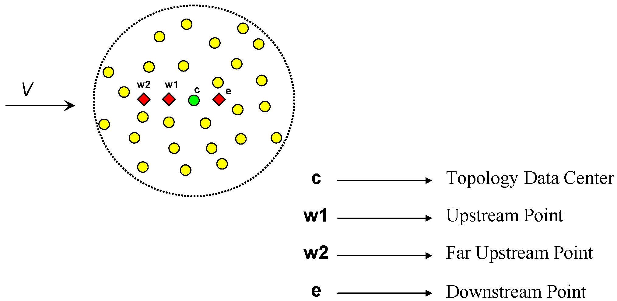
2.3. Up-Winding Schemes

In the cases when the field variable is not only diffused within the domain but convected by a flow field, $\overrightarrow{V}$, the governing equation for the field variable becomes a transport equation as:

$$\frac{\partial \varphi }{\partial t}+\left(\overrightarrow{V}\cdot \nabla \right)\varphi =\kappa {\nabla }^2\varphi$$

(34)

Special attention should be given to the convective derivative term, $(\overrightarrow{V}\cdot \nabla )\varphi$, in the event that a threshold is surpassed where the convective forces dominate the diffusion forces. A grid-based Reynolds number is employed for this purpose as:

$$R{e}_h=\frac{\left|V\right|h}{\kappa }$$

(35)

where $h$ can be assumed to be the average point spacing within the topology. The usual threshold that requires special treatment of the convective derivative is when $R{e}_h>1$, in which case an upwinded or offset derivative in the opposite direction of the flow field, $\overrightarrow{V}$, is necessary to achieve stability of the numerical solution scheme.

For example, in the case of 2D Cartesian coordinate system, the convective derivative has the following form:

$$(\overrightarrow{V}\cdot \nabla )\varphi =V_x\frac{\partial \varphi }{\partial x}+V_y\frac{\partial \varphi }{\partial y}$$

(36)

where $V_x$ and $V_y$ are the $x$ and $y$ components, respectively, of the flow field, $\overrightarrow{V}$. Concentrating on the x-direction and placing a set of virtual points in the topology as illustrated in Figure 8, three types of finite-differencing schemes for offset derivatives in the x-direction may be formulated and are given in Equations (A11)–(A13).

As it is well known, high-order finite-differencing approximation schemes are more accurate but tend to yield unnatural oscillations that can render the solution process unstable, while first-order finite-differencing approximation schemes are very stable at the expense of artificially diffusing the solution. Therefore, a blend between low- and high-order approximation schemes is necessary to compromise between accuracy and stability. In any case, all these operators can be pre-built and stored at the problem setup stage in the same way it is done for the standard differential operators discussed in previous sections, that is, for example:

$$\begin{array}{l}{\frac{\partial {\varphi }_c}{\partial x}|}_w^{1^{st}}={\left\{\partial x_w^1\right\}}^T\left\{\varphi \right\}\\ {\frac{\partial {\varphi }_c}{\partial x}|}_w^{2^{nd}}={\left\{\partial x_w^2\right\}}^T\left\{\varphi \right\}\\ {\frac{\partial {\varphi }_c}{\partial x}|}_w^{3^{rd}}={\left\{\partial x_w^3\right\}}^T\left\{\varphi \right\}\end{array}$$

(37)

where ${\left\{\partial x_w^1\right\}}^T, {\left\{\partial x_w^2\right\}}^T, \mathrm{and} {\left\{\partial x_w^3\right\}}^T$ are the first-, second-, and third-order x-derivative interpolation vectors, respectively, up-winded from the west to approximate the derivative at the topology data center, $x_c$.

A limiter is introduced to the current up-winding technique to suppress potential oscillations. Compared to the cell-based finite volume method (FVM), the LCMM is a point-based method where no cell face values are reconstructed. Hence, a direct application of the flux corrected transport (FCT) [74,75], the total variation diminishing (TVD) [76,77,78,79] or normalized variable diagrams (NVDs) [80,81,82] limiter schemes is not possible. However, the FCT, TVD, and NVDs concepts of monotonicity could be used as basis to form a limiter for the LCMM. To this end, the field variable is first evaluated at the Vvirtual points (downstream point, the data center, the upstream point, and one far upstream point) to detect if a minimum or maximum occur at the data center or upstream point, meaning that the field is not monotonic on that particular direction. If neither a minimum nor a maximum is detected at these locations no limiting action is needed and major up-winding (third-order approximation of the derivative) is performed. If a minimum or a maximum is detected at any of these locations a limiting action is introduced and minor up-winding (first-order approximation of the derivative) is performed. This minor up-winding leads to stable solutions; however, these are highly dissipative. Similar up-winding techniques were reported in [83].

3. Results

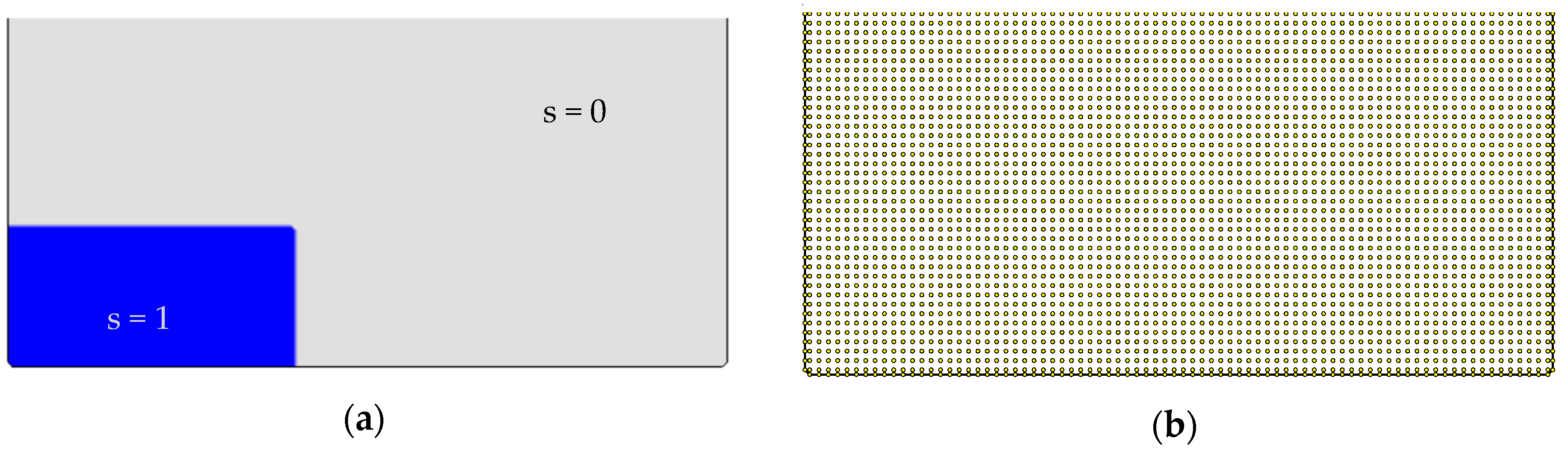
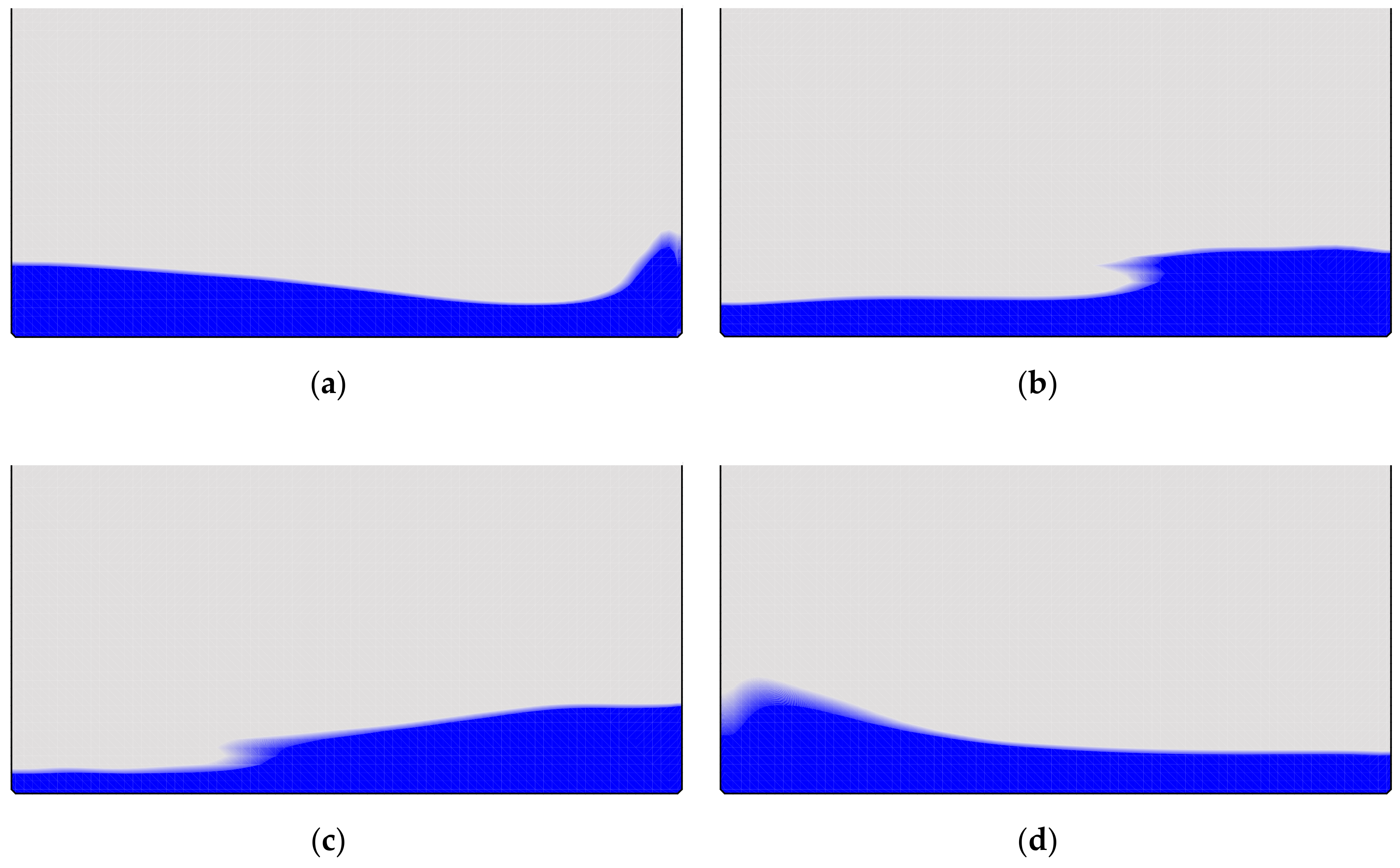
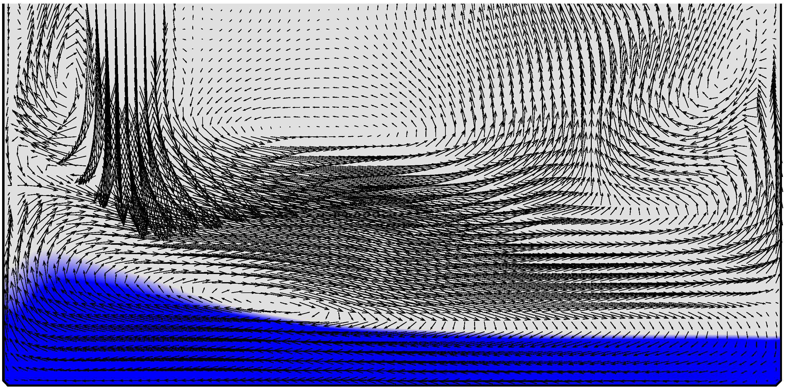
3.1. Dam-Breaking Problem

The progressive piping process is driven to a large extent by the pumping mechanism caused by transient hydrodynamics. To this end, a test of the LCMM numerical methodology is a transient hydrodynamics problem that simulates waves generated by tidal influence or hurricane force winds. The classical benchmark problem of the instantaneous dam-breaking in a “sloshing” tank was chosen for this purpose and solved using the LCMM volume of fluid (VOF) approach adopting a standard pressure-velocity correction scheme for the fluid flow problem [84,85,86,87]. This approach has been previously implemented and validated by the authors in highly-convective flows using the LCMM, see [70,71,72,73]. Here, the tank was initially filled with air $\left(s=0\right)$ everywhere except on the bottom left corner where a block of water $\left(s=1\right)$ was trapped by a dam, as seen in Figure 9a. The tank was $20\mathrm{m}$ wide by $10\mathrm{m}$ high and the initial water content was $8\mathrm{m}$ wide by $4\mathrm{m}$ high. The LCMM point distribution is also shown in Figure 9b.

The dam was instantaneously removed at $t=0$ and the water was allowed to slosh towards the right-hand side of the tank. Plots of the time-progression of the water sloshing is shown in Figure 10 for time values of $t=3,6,9,12\mathrm{s}$. A plot of the velocity vectors is shown in Figure 11 revealing the motion of the air $\left(s=0\right)$ induced by the water $\left(s=1\right)$ sloshing.

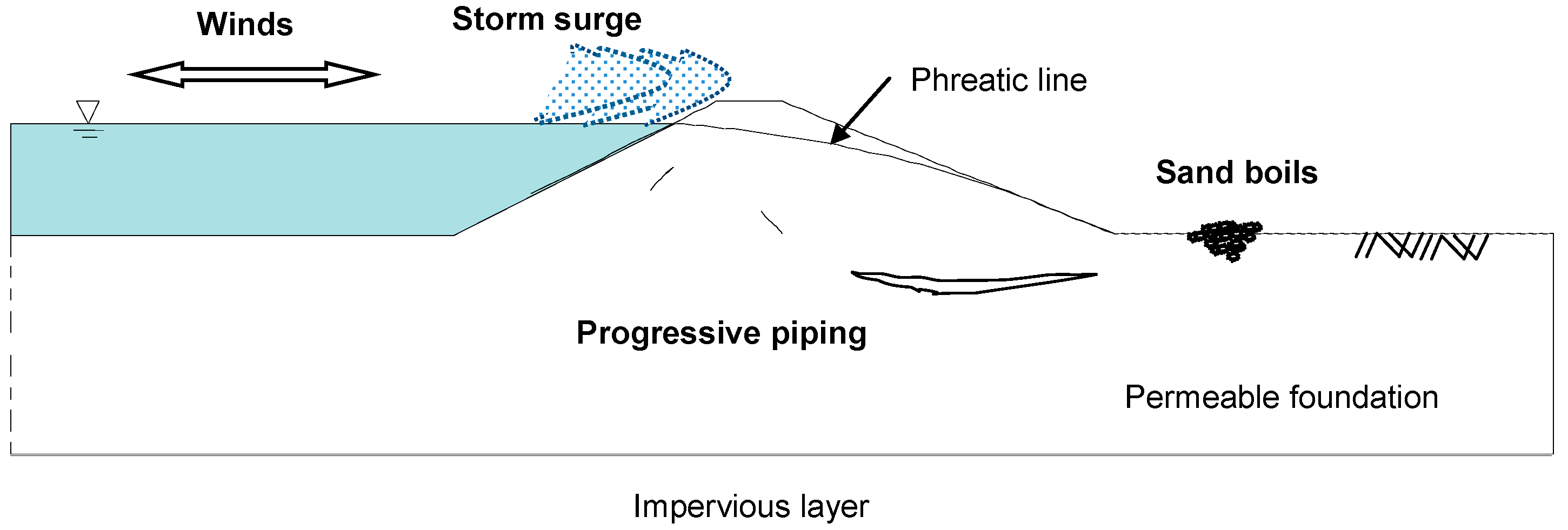
3.2. The Levee Problem

The final example deals with the problem of water flow through a compacted sand poroelastic levee. This problem combines the effects of storm surges to the levee as well as the progressive piping within the levee due to the pore pressure and stress field. The schematics of this problem are illustrated in Figure 12. The trapezoidal portion of the levee is $40\mathrm{m}$ at the base and $3\mathrm{m}$ at the top with a height of $6\mathrm{m}$. The water level on the left-hand side of the levee is $1\mathrm{m}$ from the top of the levee. A $3\mathrm{m}$-long pipe (crack) inclined 45° is included $8\mathrm{m}$ from the left-hand corner of the trapezoidal section of the levee. The levee properties where characterized as: hydraulic conductivity $K_h={10}^{-7} \mathrm{m}/\mathrm{s}$, Poisson ratio $\nu =0.35$, modulus of elasticity $E=120\mathrm{MPa}$, dry density $\rho =1500\mathrm{kg}/{\mathrm{m}}^3$, specific gravity of soil particles $SG=2.65$, and porosity $\varphi =0.3$. The water density, viscosity, and compressibility are ${\rho }_f=1000\mathrm{kg}/{\mathrm{m}}^3$, ${\mu }_f={10}^{-3} \mathrm{Pa}\cdot \mathrm{s}$, and ${\beta }_f=4.55\cdot {10}^{-10}{\mathrm{m}}^2/\mathrm{N}$, respectively. The contour plots of hydrostatic pressure levels and water flow vectors within the levee and around the pipe are shown in Figure 13 after a steady-state solution is achieved. The time progression of the saturation front within the poroelastic levee at $t=20,40,60,80,100,120$ days is shown in Figure 14.

4. Conclusions

The formation and expansion of internal voids within a water retaining structure, referred to as “progressive piping,” is a predominant cause of failure in such structures. Given that crack formation and propagation is internal to the structure, and the methods required to obtain in situ measurements, progressive piping may occur undetected. It is understood that crack expansion is dependent on hydraulic and mechanical conditions in their vicinity. Therefore, fundamental consideration of these conditions would provide insight to the mechanism of progressive piping.

To this end, the localized collocation meshless method (LCMM) is applied to the numerical analysis of pore water pressures, hydraulic gradients, and principal stresses around such cracks in levees, both here and in prior work. The LCMM formulation is an adaptation to conventional numerical techniques, leveraging localized collocation of radial basis functions to create a robust and accurate solution scheme to model poroelastic behavior through a VOF approach, while reducing the effort required to generate said model. Additionally, the LCMM scheme lends itself to the implementation of more advanced numerical formulations, such as up-winding with a limiter, to more accurately resolve the field variables in question.

The behavior of the fluid and porous media as modeled through the LCMM are used to develop a mechanistic understanding of the conditions necessary to prevent piping and to enhance the likelihood of self-healing of cracks in levees. The field results, such as principal stresses, from the enhanced LCMM approach are to be used as an input to the development of the progressive piping model. This modeling approach, used in conjunction with empirically-derived soil and erosion parameters, are used to further develop the model for progressive piping.

References

1. ICOLD. Dam Failures—Statistical Analysis; Bulletin 99; International Commission on Large Dams: Paris, France, 1995; pp. 30–31. [Google Scholar]
2. Foster, M.; Fell, R.; Spannagle, M. The statistics of embankment dam failures and accidents. Candian Geotech. J. 2000, 37, 1000–1024. [Google Scholar] [CrossRef]
3. Zaslavsky, D.; Kassiff, G. Formulation of piping mechanism in cohesive soils. Geotechnique 1965, 15, 305–316. [Google Scholar] [CrossRef]
4. Vallejo, L.E. Shear stress and the hydraulic fracturing of earth dam soils. Soils Found. 1993, 33, 14–27. [Google Scholar] [CrossRef]
5. Kakuturu, S.; Reddi, L.N. Mechanistic Model for Self-Healing of Core Cracks in Earth Dams. ASCE J. Geotech. Geoenviron. Eng. 2006, 132, 890–901. [Google Scholar] [CrossRef]
6. Zhang, L.M.; Chen, Q. Seepage failure mechanism of the Gouhou rockfill dam during reservoir water infiltration. Soils Found. 2006, 46, 557–568. [Google Scholar] [CrossRef]
7. Lakshmikantha, M.R.; Prat, P.C.; Ledesma, A. An experimental study of cracking mechanisms in drying soils. In Proceedings of the 5th ICEG Environmental Geotechnics: Opportunities, Challenges and Responsibilities, Wales, UK, 26–30 June 2006; Volume 1, pp. 533–540. [Google Scholar]
8. Watts, R.; Burk, K.; McLaren, M.; Wolfe, J.; Zender, K. Failure of the Teton dam: Geotechnical aspects. Int. Water Power Dam Constr. 2002, 54, 30–31. [Google Scholar]
9. Evans, J.E.; Scuddkr, D.M.; Gottgens, J.F.; Gill, W.M. Lessons from a Dam Failure. Ohio J. Sci. 2000, 100, 121–131. [Google Scholar]
10. Mansur, C.I.; Postol, G.; Salley, J.R. Performance of relief well systems along Mississippi River levees. J. Geotech. Geoenviron. Eng. 2000, 126, 727–738. [Google Scholar] [CrossRef]
11. Sills, G.L.; Vroman, N.D.; Wahl, R.E.; Schwanz, N.T. Overview of New Orleans levee failures: Lessons learned and their impact on national levee design and assessment. J. Geotech. Geoenviron. Eng. 2008, 134, 556–565. [Google Scholar] [CrossRef]
12. Hagerty, D.J. Piping/sapping erosion. I: Basic considerations. J. Hydraul. Eng. 1991, 117, 991–1008. [Google Scholar]
13. Hagerty, D.J. Piping/sapping erosion. II: Identification-diagnosis. J. Hydraul. Eng. 1991, 117, 1009–1025. [Google Scholar] [CrossRef]
14. Gattinoni, P.; Francani, V. A Tool for Modeling Slope Instability Triggered by Piping. World Acad. Sci. Eng. Technol. 2009, 56, 471–477. [Google Scholar]
15. Johansen, P.M.; Eikevik, J.H. Internal erosion and rehabilitation of Jukla rockfill dams. Int. Congr. Large Dams 1997, 19, 245–253. [Google Scholar]
16. Chen, C.; Liu, J.; Xia, J.; Li, Z. Integrated geophysical techniques in detecting hidden dangers in river embankments. J. Environ. Eng. Geophys. 2006, 11, 83–94. [Google Scholar] [CrossRef]
17. Sjödahl, P. Resistivity Investigation and Monitoring for Detection of Internal Erosion and Anomalous Seepage in Embankment Dams. Ph.D. Thesis, Engineering Geology, Lund University, Sweden, 2006. [Google Scholar]
18. Inazaki, T. Integrated geophysical investigation for the vulnerability assessment of earthen levee. In Proceedings of the Symposium on the Application of Geophysics to Environmental and Engineering Problems (SAGEEP), Denver, CO, USA, 1–5 April 2007. [Google Scholar]
19. Rucker, M.L.; Greenslade, M.D.; Weeks, R.E.; Fergason, K.C.; Panda, B. Geophysical and remote sensing characterization to mitigate McMicken Dam. In Proceedings of the GeoCongress 2008: Geosustainability and Geohazard Mitigation, GSP, New Orleans, LA, USA, 9–12 March 2008; Volume 178, pp. 207–214. [Google Scholar]
20. Hung, M.-H.; Lauchle, G.C.; Wang, M.C. Seepage-Induced Acoustic Emission in Granular Soils. J. Geotech. Geoenviron. Eng. 2009, 135, 566–572. [Google Scholar] [CrossRef]
21. Williams, G.W. Seepage studies using tracers and the self potential test. In Use of In Situ Tests in Geotechnical Engineering; ASCE Geotechnical Special Publication: Reston, VA, USA, 1986; Volume 6, pp. 1134–1149. [Google Scholar]
22. Holden, J. Hydrological connectivity of soil pipes determined by Ground Penetrating Radar tracer detection. Earth Surf. Process. Landf. 2004, 29, 437–442. [Google Scholar] [CrossRef]
23. Wang, X.-J.; Chen, J.-S. Research of temperature tracer method to detect tubular leakage passage in earth-dam. J. China Univ. Min. Technol. 2006, 16, 353–358. [Google Scholar]
24. Lee, J.-Y.; Kim, H.-S.; Choi, Y.-K.; Kim, J.-W.; Cheon, J.-Y.; Yi, M.-J. Sequential tracer tests for determining water seepage paths in a large rockfill dam, Nakdong River basin, Korea. Eng. Geol. 2007, 89, 300–315. [Google Scholar] [CrossRef]
25. Sellmeijer, J.B.; Koenders, M.A. A mathematical model for piping. Appl. Math. Model. 1991, 15, 646–651. [Google Scholar] [CrossRef]
26. Ojha, C.S.P.; Singh, V.P.; Adrian, D.D. Influence of porosity on piping models of levee failure. J. Geotech. Geoenviron. Eng. 2001, 127, 1071–1074. [Google Scholar] [CrossRef]
27. Ojha, C.S.P.; Singh, V.P.; Adrian, D.D. Determination of critical head in soil piping. J. Hydraul. Eng. 2003, 129, 511–518. [Google Scholar] [CrossRef]
28. Bonelli, S.; Brivois, O.; Borghi, R.; Benahmed, N. Observation, analysis and modeling in complex fluid media—On the modeling of piping erosion. C. R. Mec. 2006, 334, 555–559. [Google Scholar] [CrossRef]
29. El Shamy, U.; Aydin, F. Multi-scale modeling of flood-induced piping in river levees. J. Geotech. Geoenviron. Eng. 2008, 134, 1385–1389. [Google Scholar] [CrossRef]
30. Bonelli, S.; Brivois, O. The scaling law in the hole erosion test with a constant pressure drop. Int. J. Numer. Anal. Methods Geomech. 2008, 32, 1573–1595. [Google Scholar] [CrossRef]
31. Fell, R.; Wan, C.F.; Cyganiewicz, J.; Foster, M. Time for Development of Internal Erosion and Piping in Embankment Dams. ASCE J. Geotech. Geoenviron. Eng. 2003, 129, 307–314. [Google Scholar] [CrossRef]
32. Ozkan, S.; Adrian, D.D.; Sills, G.L.; Singh, V.P. Transient Head Development due to Flood Induced Seepage under Levees. ASCE J. Geotech. Geoenviron. Eng. 2008, 134, 781–789. [Google Scholar] [CrossRef]
33. Yi, C.; Wang, B.; Jin, M.; Guo, Z. Two-dimensional simulation of underground seepage in a dangerous piping zone of the Jingjiang Great Levee, the middle reach of the Yangtze River. Q. J. Eng. Geol. Hydrogeol. 2007, 40, 85–92. [Google Scholar] [CrossRef]
34. Kakuturu, S.; Reddi, L.N. Evaluation of the Parameters Influencing Self-Healing in Earth Dams. ASCE J. Geotech. Geoenviron. Eng. 2006, 132, 879–889. [Google Scholar] [CrossRef]
35. Belytscho, T.; Lu, Y.Y.; Gu, L. Element-free Galerkin methods. Int. J. Numer. Methods 1994, 37, 229–256. [Google Scholar] [CrossRef]
36. Atluri, S.N.; Shen, S. The Meshless Method; Tech. Science Press: Henderson, NV, USA, 2002. [Google Scholar]
37. Atluri, S.N.; Zhu, T. A new meshless local Petrov-Galerkin (MLPG) approach in computational mechanics. Comput. Mech. 1998, 22, 117–127. [Google Scholar] [CrossRef]
38. Onate, E.; Idehlson, S.; Zienkiewicz, O.C.; Taylor, R.L.; Sacco, C. A stabilized finite point method for analysis of fluid mechanics problems. Comput. Methods Appl. Mech. Eng. 1996, 139, 315–346. [Google Scholar] [CrossRef]
39. Liu, G.R. Mesh Free Methods: Moving Beyond the Finite Element Method; CRC Press: Boca Raton, FL, USA, 2002. [Google Scholar]
40. Melenk, J.M.; Babuska, I. The partition of unity finite element method: Basic theory and application. Comput. Meth. Appl. Mech. Eng. 1996, 139, 289–316. [Google Scholar] [CrossRef]
41. Gu, Y.T.; Liu, G.R. Meshless techniques for convection dominated problems. Comput. Mech. 2006, 38, 171–182. [Google Scholar] [CrossRef]
42. Gottlieb, D.; Orzag, S.A. Numerical Analysis of Spectral Methods: Theory and Applications; Society for Industrial and Applied Mathematics: Bristol, UK, 1977. [Google Scholar]
43. Maday, Y.; Quateroni, A. Spectral and Pseudo-Spectral Approximations of the Navier-Stokes Equations. SIAM J. Numer. Anal. 1982, 19, 761–780. [Google Scholar] [CrossRef]
44. Patera, A. A Spectral Element Method of Fluid Dynamics: Laminar flow in a channel expansion. J. Comput. Phys. 1984, 54, 468–488. [Google Scholar] [CrossRef]
45. Macaraeg, M.; Street, C.L. Improvement in Spectral Collocation Discretization through a Multiple Domain Technique. Appl. Numer. Math. 1986, 2, 95–108. [Google Scholar] [CrossRef]
46. Hwar, C.K.; Hirsch, R.; Taylor, T.; Rosenberg, A.P. A Pseudo-Spectral Matrix Element Method for Solution of Three Dimensional Incompressible Flows and its Parallel Implementation. J. Comput. Phys. 1989, 83, 260–291. [Google Scholar]
47. Fasshauer, G. RBF Collocation Methods as Pseudo-Spectral Methods. Boundary Elements XVII; Kassab, A., Brebbia, C.A., Divo, E., Eds.; WIT Press: Billerica, MA, USA, 2005; pp. 47–57. [Google Scholar]
48. Powell, M.J.D. The Theory of Radial Basis Function Approximation. In Advances in Numerical Analysis; Light, W., Ed.; Oxford Science Pub.: Oxford, UK, 1992; Volume 2, pp. 143–167. [Google Scholar]
49. Buhmann, M.D. Cambridge Radial Basis Functions: Theory and Implementation; Cambridge University Press: Cambridge, UK, 2003. [Google Scholar]
50. Dyn, N.; Levin, D.; Rippa, S. Numerical Procedures for Surface Fitting of Scattered Data by Radial Basis Functions. SIAM J. Sci. Stat. Comput. 1986, 7, 639–659. [Google Scholar] [CrossRef]
51. Hardy, R.L. Multiquadric Equations of Topography and Other Irregular Surfaces. J. Geophys. Res. 1971, 176, 1905–1915. [Google Scholar] [CrossRef]
52. Kansa, E.J. Multiquadrics—A scattered data approximation scheme with applications to computational fluid dynamics I-surface approximations and partial derivative estimates. Comput. Math. Appl. 1990, 19, 127–145. [Google Scholar] [CrossRef]
53. Kansa, E.J. Multiquadrics- a scattered data approximation scheme with applications to computational fluid dynamics II-solutions to parabolic, hyperbolic and elliptic partial differential equations. Comput. Math. Appl. 1990, 19, 147–161. [Google Scholar] [CrossRef]
54. Kansa, E.J.; Hon, Y.C. Circumventing the Ill-Conditioning Problem with Multiquadric Radial Basis Functions: Applications to Elliptic Partial Differential Equations. Comput. Math. Appl. 2000, 39, 123–137. [Google Scholar] [CrossRef]
55. Franke, R. Scattered data interpolation: Test of some methods. Math. Comput. 1982, 38, 181–200. [Google Scholar]
56. Mai-Duy, N.; Tran-Cong, T. Mesh-Free Radial Basis Function Network Methods with Domain Decomposition for Approximation of Functions and Numerical Solution of Poisson’s Equation. Eng. Anal. Bound. Elem. 2002, 26, 133–156. [Google Scholar] [CrossRef]
57. Cheng, A.H.-D.; Golberg, M.A.; Kansa, E.J.; Zammito, G. Exponential Convergence and H-c Multiquadric Collocation Method for Partial Differential Equations. Numer. Methods Part Differ. Equ. 2003, 19, 571–594. [Google Scholar] [CrossRef]
58. Sarler, B.; Vertnik, R. Local Explicit Radial Basis Function Collocation Method for Diffusion Problems. Comput. Math. Appl. 2006, 51, 1269–1282. [Google Scholar] [CrossRef]
59. Vertnik, R.; Sarler, B. Meshless local radial basis function collocation method for convective-diffusive solid-liquid phase change problems. Int. J. Numer. Methods Heat Fluid Flow 2006, 16, 617–640. [Google Scholar] [CrossRef]
60. Vertnik, R.; Zaloznik, M.; Sarler, B. Solution of transient direct-chill aluminium billet casting problem with simultaneous material and interphase moving boundaries by a meshless method. Eng. Anal. Bound. Elem. 2006, 30, 847–855. [Google Scholar] [CrossRef]
61. Divo, E.; Kassab, A.J. A Meshless Method for Conjugate Heat Transfer Problems. Eng. Anal. 2005, 29, 136–149. [Google Scholar] [CrossRef]
62. Gerace, S.A.; Divo, E.; Kassab, A.J. A Localized Radial-Basis-Function Meshless Method Approach to Axisymmetric Thermo-Elasticity. In Proceedings of the 9th AIAA/ASME Joint Thermophysics and Heat Transfer Conference 2006, San Francisco, CA, USA, 5–8 June 2006. [Google Scholar]
63. Divo, E.; Kassab, A.J. Iterative Domain Decomposition Meshless Method Modeling of Incompressible Flows and Conjugate Heat Transfer. Eng. Anal. 2006, 30, 465–478. [Google Scholar] [CrossRef]
64. Divo, E.; Kassab, A.J. An Efficient Localized RBF Meshless Method for Fluid Flow and Conjugate Heat Transfer. ASME J. Heat Transf. 2007, 129, 124–136. [Google Scholar] [CrossRef]
65. Divo, E.; Kassab, A.J. Localized Meshless Modeling of Natural Convective Viscous Flows. Numer. Heat Transf. Part A Fundam. 2008, 53, 487–509. [Google Scholar] [CrossRef]
66. Erhart, K.; Kassab, A.J.; Divo, E. An Inverse Localized Meshless Technique for the Determination of Non-Linear Heat Generation Rates in Living Tissues. Int. J. Numer. Methods Heat Fluid Flow 2008, 18, 401–414. [Google Scholar] [CrossRef]
67. El Zahab, Z.; Divo, E.; Kassab, A.J. A Localized Collocation Meshless Method (LCMM) for Incompressible Flows CFD Modeling with Applications to Transient Hemodynamics. Eng. Anal. Bound. Elem. 2009, 33, 1045–1061. [Google Scholar] [CrossRef]
68. El Zahab, Z.; Divo, E.; Kassab, A. Minimization of the Wall Shear Stress Gradients in Bypass Grafts Anastomoses using Meshless CFD and Genetic Algorithms Optimization. Comput. Methods Biomech. Biomed. Eng. 2010, 13, 35–47. [Google Scholar] [CrossRef] [PubMed]
69. Divo, E.; Kassab, A.J.; Reddi, L.; Kakuturu, S.; Hagen, S. RBF-FVM Numerical Solution of the Poro-Elasticity Levee Problem with Time-Varying Boundary Conditions. In Proceedings of the ECCOMAS Couple Problems 2009, Ischia Island, Italy, 8–10 June 2009. [Google Scholar]
70. Gerace, S.; Erhart, K.; Divo, E.; Kassab, A.J. Adaptively Refined Hybrid Meshless Scheme with Applications to High-Speed Turbulent Flow. Comput. Model. Eng. Sci. 2011, 1927, 1–33. [Google Scholar]
71. Bear, J. Dynamics of Fluids in Porous Media; Dover Publications, Inc.: New York, NY, USA, 1988. [Google Scholar]
72. Wang, H.F.; Anderson, M.P. Introduction to Groundwater Modeling: Finite and Finite Element Methods; W.H. Freeman and Company: San Francisco, CA, USA, 1982. [Google Scholar]
73. Hirt, C.W.; Nichols, B.D. Volume of Fluid (VOF) Method for the Dynamics of Free Boundaries. J. Comput. Fluids 1981, 39, 201–225. [Google Scholar] [CrossRef]
74. Leonard, B.P. A stable and accurate convective modelling procedure based on quadratic interpolation. Comput. Methods Appl. Mech. Eng. 1979, 19, 59–98. [Google Scholar] [CrossRef]
75. Borris, J.P.; Book, D.L. Flux-corrected transport II: Generalizations of the method. J. Comput. Phys. 1983, 18, 248. [Google Scholar]
76. Harten, A. High resolution schemes for hyperbolic conservation laws. J. Comput. Phys. 1983, 49, 357–393. [Google Scholar] [CrossRef] [Green Version]
77. Van Leer, B. Towards the ultimate conservative difference scheme. V. A second order sequel to Godunov’s method. J. Comput. Phys. 1979, 32, 101–136. [Google Scholar] [CrossRef]
78. Chakravarthy, S.R.; Osher, S. High resolution applications of the OSHER upwind scheme for the Euler equations. In Proceedings of the 6th Computational Fluid Dynamics Conference Danvers, Danvers, MA, USA, 13–15 July 1983. [Google Scholar]
79. Roe, P.L. Some contributions to the modelling of discontinuous flows. Lect. Appl. Math. 1985, 22, 163–193. [Google Scholar]
80. Gaskell, P.H.; Lau, A.K.C. Curvature compensated convective transport: SMART, a new boundedness preserving transport algorithm. Int. J. Numer. Methods Fluids 1988, 8, 617–641. [Google Scholar] [CrossRef]
81. Leonard, B.P. The ULTIMATE conservative difference scheme applied to unsteady one-dimensional advection. Comput. Methods Appl. Mech. Eng. 1991, 88, 17–74. [Google Scholar] [CrossRef]
82. Jasak, H.; Weller, H.G.; Gosman, A.D. High resolution NVD differencing scheme for arbitrary unstructured meshes. Int. J. Numer. Methods Fluids 1999, 31, 431–449. [Google Scholar] [CrossRef]
83. Chandhini, G.; Sanyasiraju, Y.V.S. Local RBF-FD solutions for steady convection–diffusion problems. Int. J. Numer. Methods Eng. 2007, 72, 352–378. [Google Scholar] [CrossRef]
84. Harlow, F.H.; Welch, J.E. Numerical Calculation of time dependent viscous incompressible flow of fluids with a free surface. Phys. Fluids 1965, 8, 2182–2189. [Google Scholar] [CrossRef]
85. Patankar, S.V. Numerical Heat Transfer and Fluid Flow; Hemisphere Press: Coral Gables, FL, USA, 1980. [Google Scholar]
86. Kim, D.; Choi, H. A Second-order time-accurate finite volume method for unsteady incompressible flow on hybrid unstructured grids. J. Comput. Phys. 2000, 162, 411–428. [Google Scholar] [CrossRef]
87. Zhang, Y.; Street, R.L.; Koseff, J.R. A Non-staggered grid, fractional step method for time-dependent incompressible Navier-Stokes equations in curvilinear coordinates. J. Comput. Phys. 1994, 114, 18–33. [Google Scholar] [CrossRef]
Figure 1. Experiments for observing progressive piping: (a) Schematic of the setup, (b,c) flow cells with simulated cracks.
Fluids 04 00120 g001
Figure 2. Schematic of flow cells for estimation of model parameters associated with (a) dislodgement of particles in the upstream part, (b) erodibility of crack walls, and (c) particle entrapment capacity of soil in the downstream side of crack.
Fluids 04 00120 g002
Figure 3. Scattered point distribution in generalized domain.
Fluids 04 00120 g003
Figure 4. Collocation topology for internal, boundary, and corner data centers.
Fluids 04 00120 g004
Figure 5. Collocation topology selection on a non-uniform point distribution.
Fluids 04 00120 g005
Figure 6. Distribution of internal shadow points to compute normal derivatives.
Fluids 04 00120 g006
Figure 7. Illustration of a topology with virtual points around the data center, x c .
Fluids 04 00120 g007
Figure 8. Localized topology with virtual point distribution for up-winding schemes.
Fluids 04 00120 g008
Figure 9. Schematics of (a) the initial condition and (b) LCMM point distribution of the dam-breaking problem.
Fluids 04 00120 g009
Figure 10. Time-progression of dam-breaking problem at (a) t = 3 s, (b) t = 6 s, (c) t = 9 s, (d) t = 12 s.
Fluids 04 00120 g010
Figure 11. Velocity vector plot of the dam-breaking problem solution at t = 12   s .
Fluids 04 00120 g011
Figure 12. Schematics of the groundwater flow through a poroelastic sand levee problem.
Fluids 04 00120 g012
Figure 13. Contour plots of hydrostatic pressure levels and water flow vectors within the levee.
Fluids 04 00120 g013
Figure 14. Time progression of the saturation front in the poroelastic levee at (a) t = 20 days, (b) t = 40 days, (c) t = 60 days, (d) t = 80 days, (e) t = 100 days, and (f) t = 120 days.
Fluids 04 00120 g014