1. Introduction
Vehicle emissions on highways can lead to air pollution and some symptoms of disease in people, especially young children, who live in the proximity of heavily trafficked highways [
1].
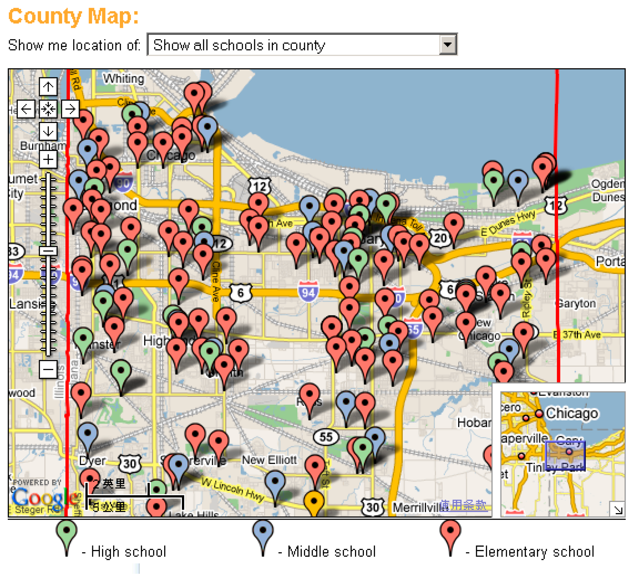
Figure 1 is a Google Maps search result of schools in Lake County, Indiana, where many schools are located near highways. Previous research showed that vehicle emissions could cause prematurity and low birth weight among mothers [
2] and respiratory problems to residents [
3]. Air pollution has been a serious global issue. One major source of air pollutants is vehicle emissions, which contain toxic nitrogen oxides (NO
x), carbon monoxide (CO), and particle matter (PM). According to the Environmental Protection Agency (EPA), vehicles that are larger, heavier, and more powerful generally, have lower fuel economy and higher CO
2 emissions than other comparable vehicles. The mix of vehicles in the sedans/wagons vehicle type have an average weight that is still 13% below 1975 values, but trucks are now almost 30% heavier than in model year 1975. Vehicle power and acceleration have increased across all vehicle types [
4]. It is important to study automobile-induced highway emission dispersion.
Highway noise barriers were originally designed to protect communities near highways from vehicle noise. Recent study has suggested that roadside barriers have positive effects on reducing downstream emission concentration. The level of reduction can be determined by a variety of factors, such as roadway configuration, local meteorology, barrier height and other factors [
5].
A commonly cited study is the wind tunnel study published by Heist et al., 2009 [
6]. They modeled 12 different roadway configurations, including noise barriers and roadway elevation or depression, and discussed the effect of those configurations on the dispersion of traffic emission. The study concluded that all 12 configurations reduced the downstream near-ground concentration compared with that for a flat and unobstructed roadway [
6]. Amini et al., 2016, found that a 4 m high barrier resulted in a 35% reduction in average concentration within 40 m of the barrier, relative to the no-barrier site. Also, the concentration reduction could be 55% if the barrier height was doubled [
7]. Previous research also focused on noise barrier side edge effects under different thermal conditions, but only rectangular noise barriers were studied [
8].
Because noise barriers are designed to suppress the spread of noise, the way noise barriers affect emissions dispersion is different than the way they impede sound propagation, so governing equations and mechanisms are completely different. A lot of research has focused on the acoustic performance of barriers with different shapes and surface conditions [
9,
10,
11,
12,
13]. Scholes et al. carried out field research to obtain the acoustic performance of full-scale noise barriers of various heights under a range of wind conditions [
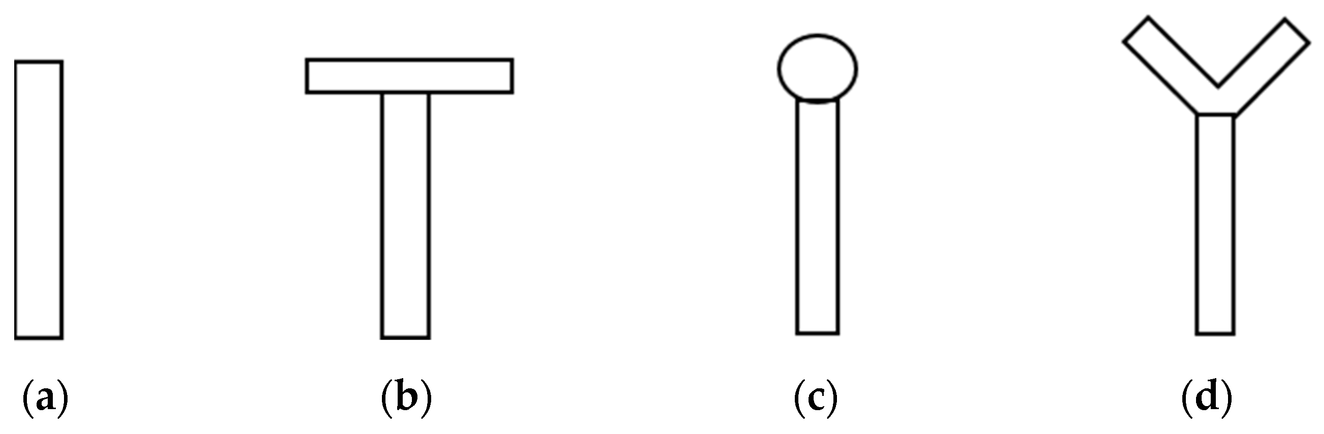
9]. Ishizuka and Fujiwara introduced a different type of commonly used noise barrier in their paper [
10], as shown in
Figure 2. They tested the acoustic performance of common noise barriers using the boundary element method (BEM) and suggested that the soft T-shaped barrier had the best results in noise reduction. Baulac et al. analyzed the acoustical efficiency of T-shaped noise barriers whose top is covered with a series of wells [
11]. Unfortunately, the study of barrier shape effect was limited on acoustic performance. To the best of the authors’ knowledge, there was no further study about the noise barrier shape effect on highway emission dispersion in the literature.
Besides field study and wind tunnel testing, numerical simulation has become prevalent due to the rapid development of computational resources and techniques. A numerical study by Hagler et al., 2011 [
14], matched the previous wind tunnel study. Their results further implied that roadside barriers may mitigate near-road air pollution. Furthermore, Finn et al. [
15], conducted a roadway toxics dispersion study to document the effects on concentrations of roadway emissions behind a roadside sound barrier in various conditions of atmospheric stability; and Steffens et al. [
16], modeled a solid noise barrier under various atmospheric stability conditions by employing Reynolds Averaged Navier-Stokes (RANS) and Large Eddy Simulation (LES) models.
As mentioned above, the level of pollutant reduction can be determined by the local meteorology and inflow conditions. Three inflow conditions were adopted in this study: (1) uniform inlet wind profile without wind shear, which is commonly used in wind tunnel testing; (2) linear wind shear profile, which has the same mass flow rate as the uniform inlet wind profile; (3) normal wind profile, steady vertical wind shear, which uses a power law velocity profile [
17]. The existence of wind shear could create a very complex wake structure with substantial asymmetries, streamwise vorticity generation, and non-periodicities [
18]. Consequently, the wake and turbulence were expected to influence the emission dispersion downstream.
In this paper, ANSYS®Fluent 19.2 (Ansys Inc., Canonsburg, PA, USA) was applied to simulate noise barrier shape effects on the emission dispersion on the highway and in the downstream region. The influences from different inflow conditions on the emission dispersion were also analyzed.
2. Materials and Methods
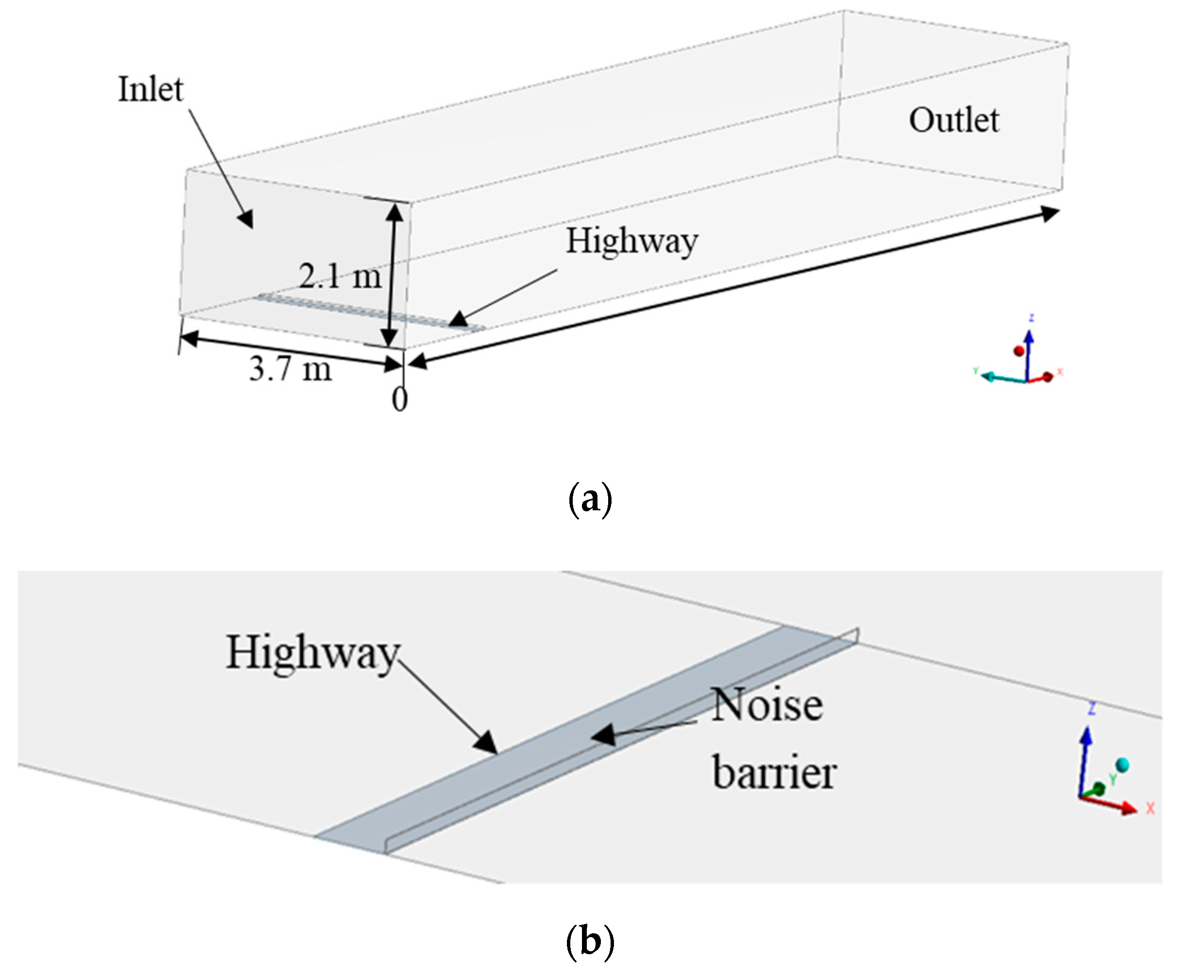
The model configuration followed the wind tunnel experiment conducted by Heist et al. [
6]. The wind tunnel was a 1:150 model (18.3 m × 3.7 m × 2.1 m), and the tracer gas ethane (C
2H
6) represented the automobile emission on the highway. The noise barrier was 6 m high (H) in the full scale and spanned along the highway. The wind tunnel experiments modeled 12 different roadway configurations in total, for validation study one configuration was adopted.
The computational domain in this paper was not in the full scale considering the whole computational time. Instead, the computational domain was also a 1:150 model and had the same dimensions as those for the wind tunnel. The x-axis was extended along with the wind direction perpendicular to the highway. The highway was 2 m away from the inlet and treated as the emission source. The highway noise barrier was 0.04 m high, 0.003 m thick (6 m high, 0.5 m thick in the full scale). The computational domain is shown in
Figure 3.
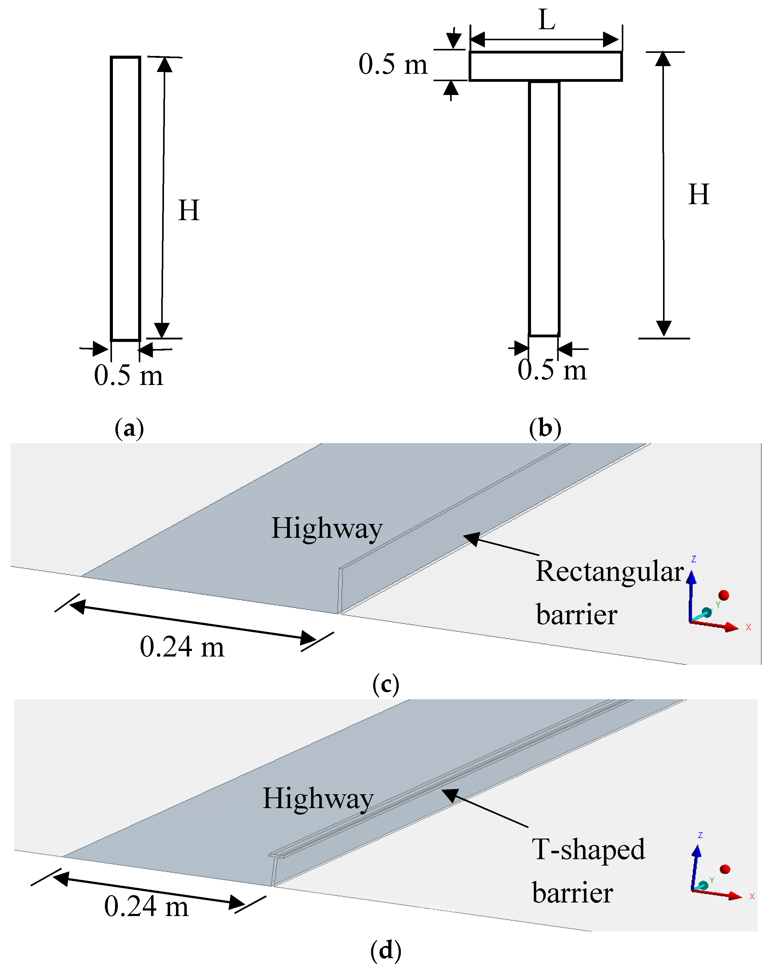
Different shapes of noise barrier in this study are classified by the cross-sectional geometry. The profiles of noise barrier are shown in
Figure 4, which shows the full-scale dimensions. All barriers would become a 1:150 model in the computational domain.
The rectangular noise barrier has one critical parameter, i.e., height H. The T-shaped noise barrier, however, has an additional important parameter, i.e., top length L. For T-shaped noise barriers, a ratio of the top length to the height, L/H, becomes a dimensionless parameter. In order to study the shape effects, four T-shaped and one rectangular barrier were tested. The dimensions are detailed in
Table 1. The thickness of the noise barrier in all simulation cases is 0.5 m.
Commercial software ANSYS
®Fluent 19.2 (Ansys Inc., Canonsburg, PA, USA) was used in the numerical simulation. RANS averages parameters in N-S equations on time and simulates all the turbulence scales; LES averages the parameters on space so that large eddies could satisfy governing equations and simulate only the smallest eddies. Reynolds Averaged Navier-Stokes modeling is a widely used scheme for simulating turbulent flow because it is relatively accurate and computationally efficient compared to Large Eddy Simulation. RANS modelling is selected in this paper with a consideration for timesaving. RANS equation is expressed as [
19]:
Different turbulence models, including standard/RNG/realizable k-ε model and standard/SST k-ω model were tested in this study. The major differences in three k-ε models are the method of calculating turbulent viscosity, the turbulent Prandtl numbers governing the turbulent diffusion of k and ε, and the generation and destruction terms in the ε equation [
20]. The major differences in two k-ω models are the gradual change from the standard k-ω model in the inner region of the boundary layer to a high-Reynolds number version of the k-ε model in the outer part of the boundary layer, and the modified turbulent viscosity formulation to account for the transport effects of the principal turbulent shear stress [
21]. The simulation results were compared at the beginning in order to find a better model that can give valid results. Finally, the realizable k-ε model with turbulent Schmidt number of 1.0 was selected due to its best match with the wind tunnel experimental data.
The governing equations for the turbulence kinetic energy, k, and the turbulence dissipation rate, ε, in the realizable k-ε model are described as [
22]:
and
where
The non-reaction species transport model was able to simulate transportation and dispersion of various species. Carbon monoxide (CO) was selected as the representative of automobile emissions and defined as an emission source on the highway in this paper. A mixture of air and CO was regarded as the material in the whole computational domain. The concentration of CO was normalized to a dimensionless concentration [
6]:
where
are length and width of the emission source, which are 0.24 m and 3.7 m respectively. Reference velocity
is 2.46 m/s. Volumetric flow rate
is 1500 cc/min.
The general form in the non-reaction species transport equations for the
ith species is expressed as [
23]:
is equal to 0 in this study due to no chemical reactions occurring in the computational domain.
The inflow condition was the power law profile, which is widely used to describe the wind profile. The power law at constant temperature (300 K) was integrated to define the incoming wind profile. The power law represents a simple model for the vertical wind speed profile [
24]. The equation is defined as:
In the full scale, the reference velocity at the reference height of 30 m was 2.46 m/s [
6]. The power law exponent α was generally defined as a constant, here 1/7 power law is implemented. Afterwards, the other three different inflow conditions [
17] were used to study the influence of inflow conditions.
Boundary conditions applied in the computational domain were listed in
Table 2. The inlet is a velocity inlet, and the velocity is determined either by a user-defined function or by a constant number. The outlet is defined as outflow. The highway is regarded as the automobile emissions source and defined as a mass flow inlet. The magnitude is the product of volumetric flow rate multiplied by density. The emission gas in this paper is CO whose density is 1.165 kg/m
3. The volumetric flow rate is 1500 cc/min given by the wind tunnel study [
6]. Therefore, the mass flow rate is 2.9 × 10
−5 kg/s. In this paper, the bottom surface represents the ground and is considered a stationary and very smooth wall. Noise barriers are also stationary and smooth walls. The top and other two side surfaces are symmetry boundary conditions.
3. Results
The results from the numerical simulation were first validated with the wind tunnel experiment. The main results in this paper included noise barrier shape effects and influence of inflow conditions. The representative automobile emission in this paper is carbon monoxide (CO). The whole numerical simulation domain is the mixture of carbon monoxide and air. The concentration of CO would have been expected to decrease if other automobile emission elements were included. All results were reflected in contours of CO molar concentration and vertical distribution of CO normalized concentration at different locations.
3.1. Mesh Independent Study
In order to study how mesh size would influence the results, three sets of mesh of the base case were tested. The realizable k-ε turbulence model was used. Face sizing was inserted onto highway face and noise barrier surfaces. Different mesh size, thus, could be obtained by modifying the element size of mesh and face size.
Table 3 lists the number of cells and nodes for each mesh. The smallest cell number means the coarsest mesh, and the largest cell number means the finest mesh.
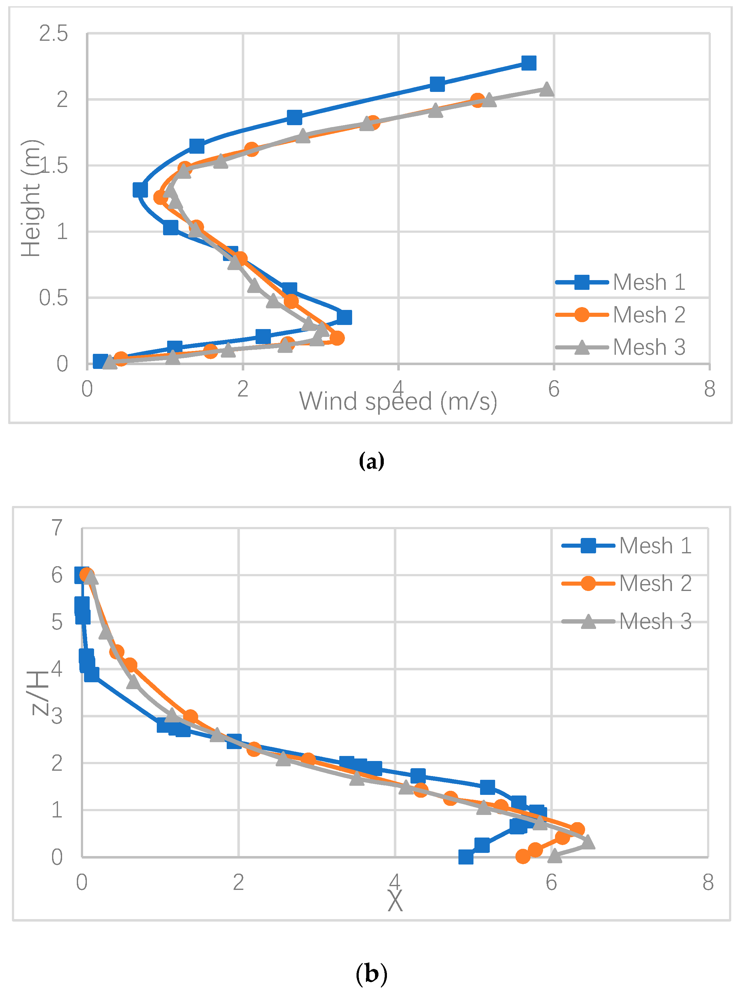
Three sets of meshes were tested in this study. Results of velocity profiles and the vertical distribution of the normalized concentration at x/H = 5 were compared by using the three sets of meshes, as shown in
Figure 5. Steady state simulation results from mesh 2 and 3 were very close, while those from mesh 1 deviated from the other two slightly. The mesh with large elements cell number increased simulation accuracy, but also prolonged computational time. Therefore, the mesh with the medium cell number, mesh 2, was selected for later simulation, which brought a better balance in computational accuracy and computing time.
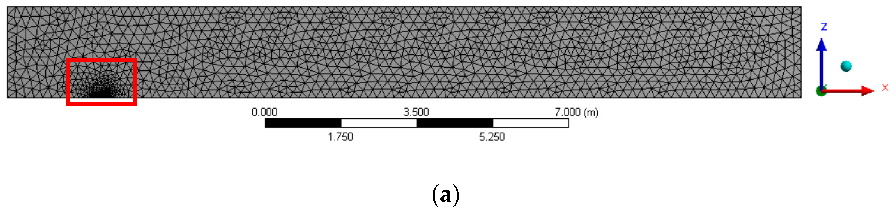
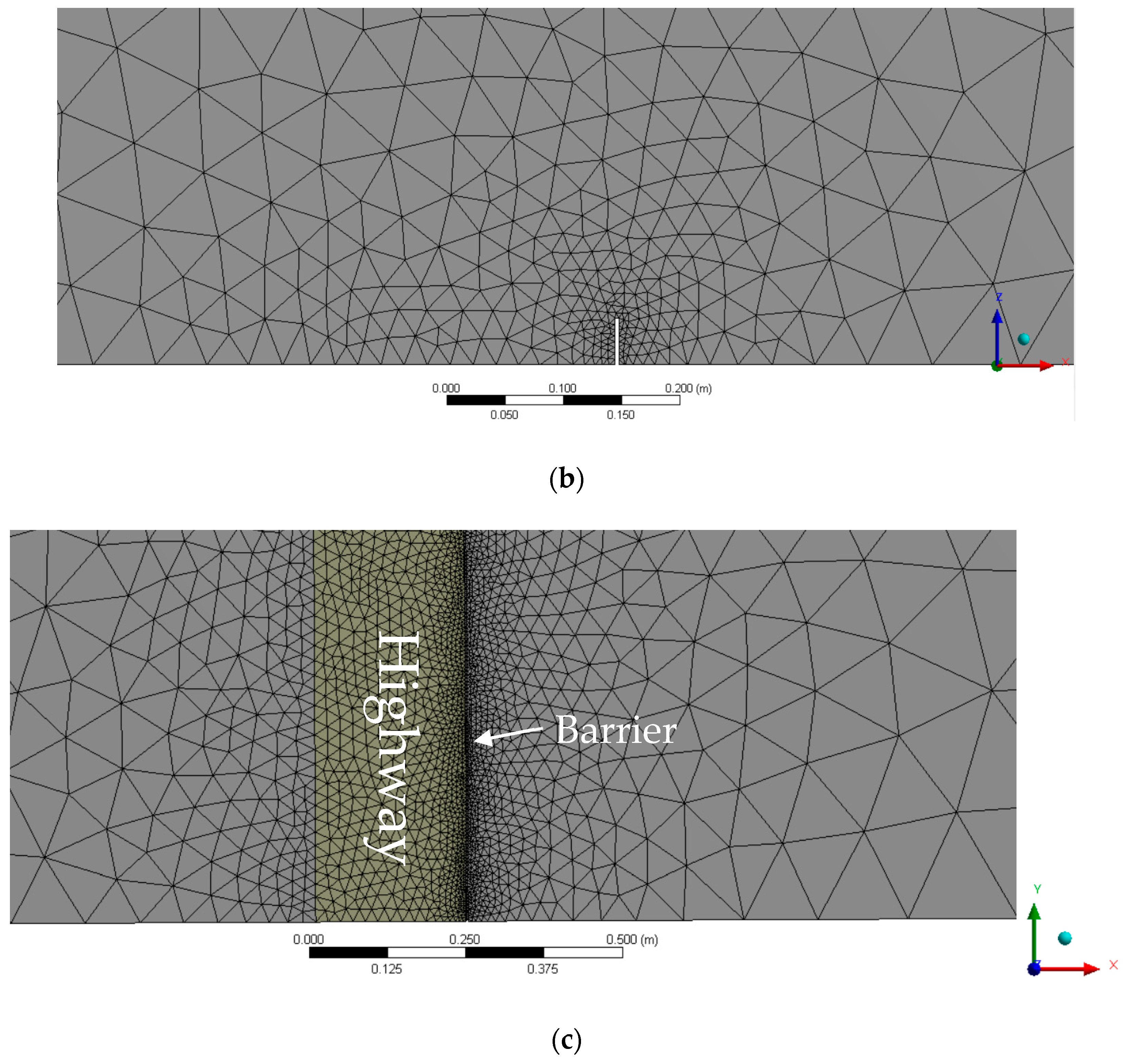
Mesh 2 is shown in
Figure 6.
Figure 6a is the front view of the overall computational mesh.
Figure 6b is the close-up front view and (c) is the close-up bottom view of the meshes around the noise barrier and highway. The clustered meshes around the noise barrier and highway can be seen clearly, which can resolve the flow features accurately near the highway and noise barrier.
3.2. Turbulence Model Selection
The numerical model was validated with the wind tunnel study by comparing the vertical distribution of the emission concentration at the location x/H = 5 (5 times noise barrier height far behind the barrier). The base case in this study was compared with one of 12 configurations in the wind tunnel study. The reference configuration is a flat highway along with a single 6 m high rectangular noise barrier. Note that the tracer gas in the wind tunnel study is ethane (C
2H
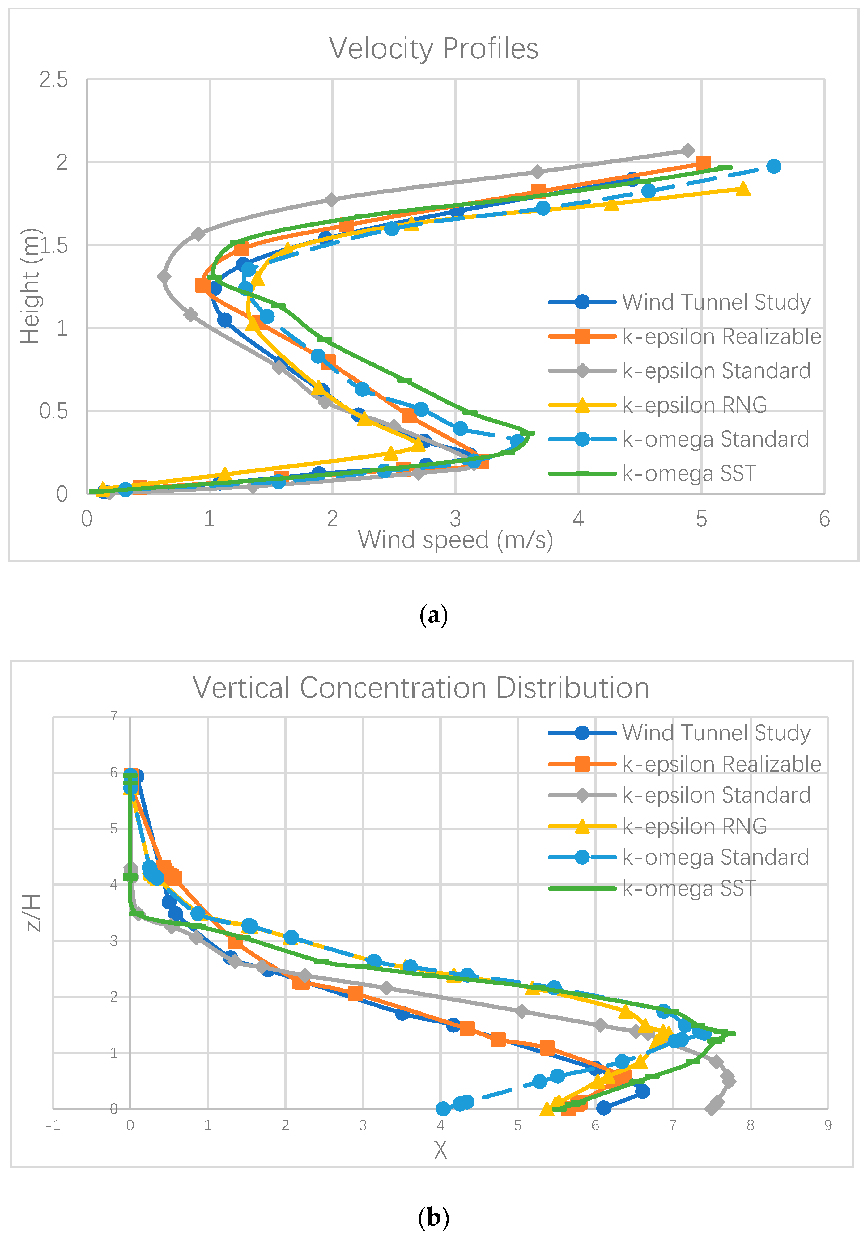
6). The mesh 2, with grid points 121,383 was used for the following calculation. All results obtained by realizable/standard/RNG k-ε and standard/SST k-ω turbulence models are shown in
Figure 7.
In
Figure 7a, the biggest differences between each model were at two turning points where the realizable k-ε model matched better with the wind tunnel study. In
Figure 7b, all turbulence models matched well with the wind tunnel study in the high altitude (z/H ≥ 3; higher than 3 times noise barrier height). However, in the near-ground region (z/H ≤ 3), the result for each turbulence model varied a lot. This study focused more on the near-ground region because there are many communities and buildings that are located near highways. Under z/H = 3, the realizable k-ε model matched better with the wind tunnel study. Consequently, the realizable k-ε model was used in the following simulation for T-shaped noise barriers.
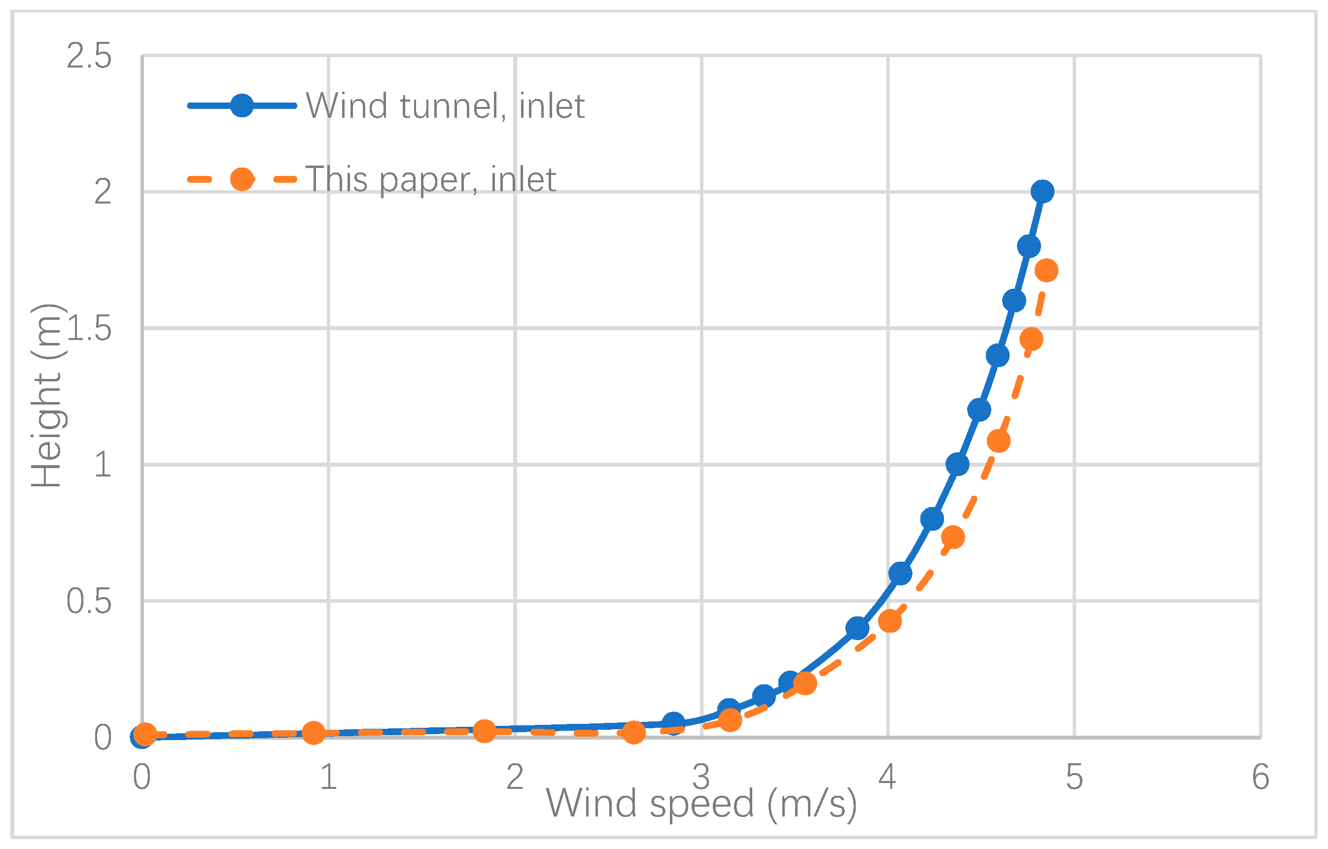
Secondly, the inlet velocity was determined by the power law. The air flow speed in the wind tunnel study was fixed at 4.7 m/s at a height of 165 cm [
6]. The wind velocity profile at inlet is shown in
Figure 8.
The wind profile in this paper matched that used in the wind tunnel study. Overall good agreement can be observed.
3.3. Noise Barrier Shape Effects
This paper used CO to represent the automobile emissions. Five configurations listed in
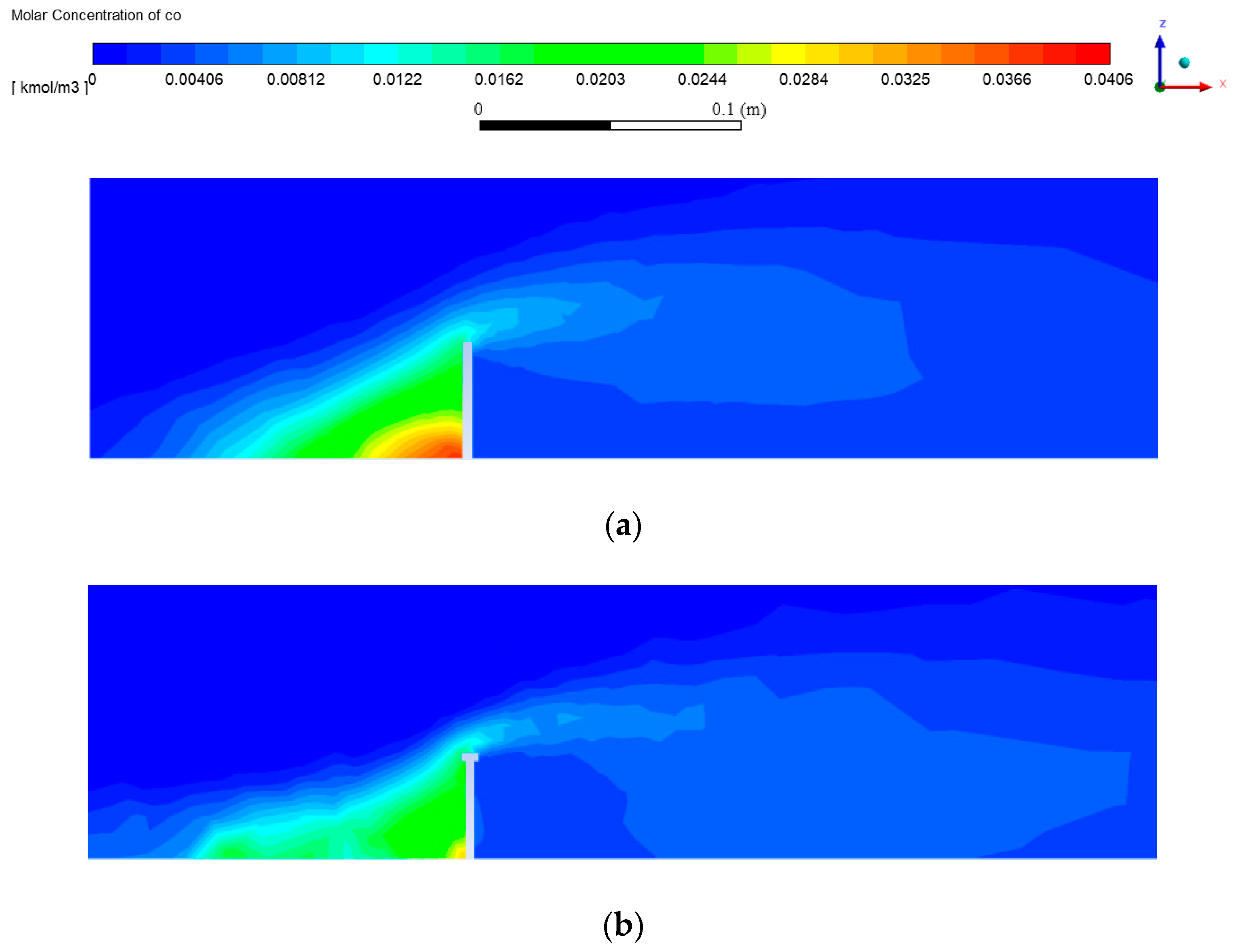
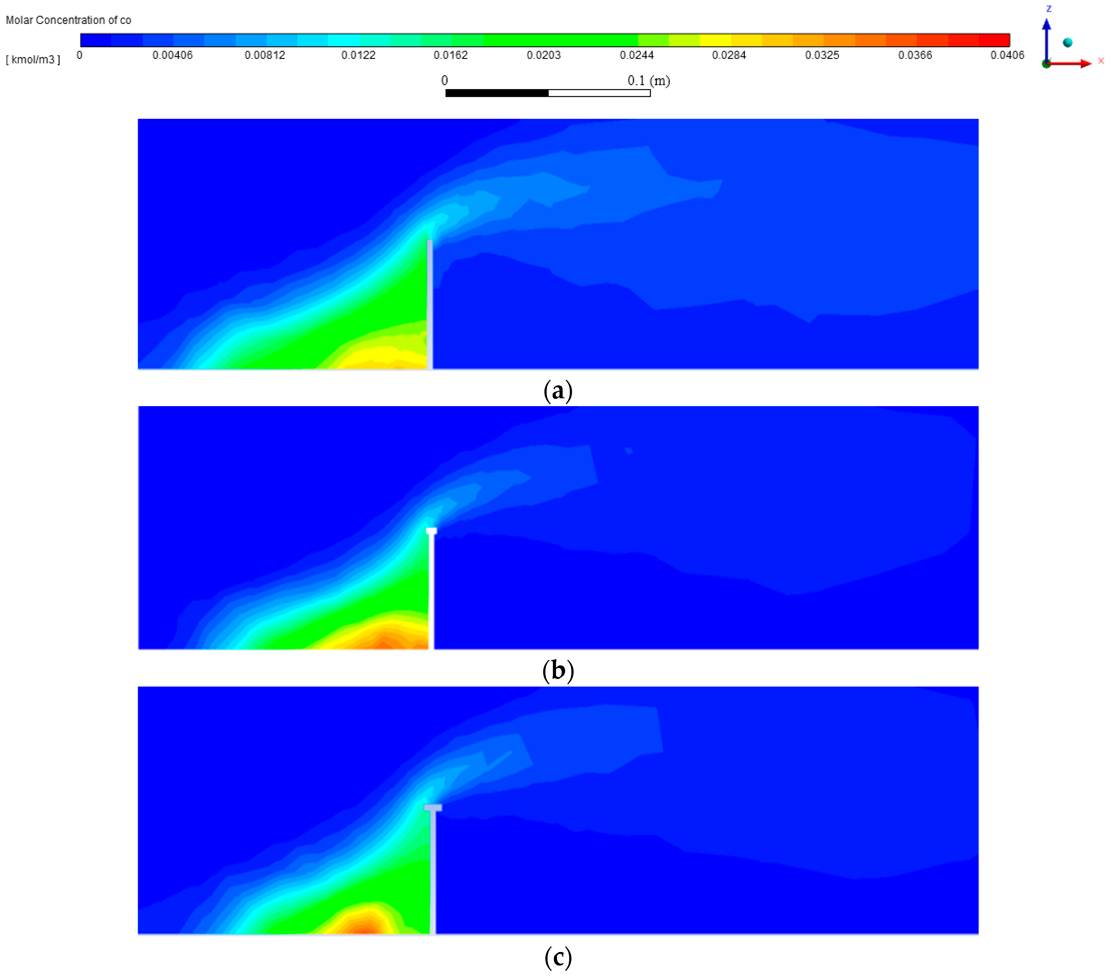
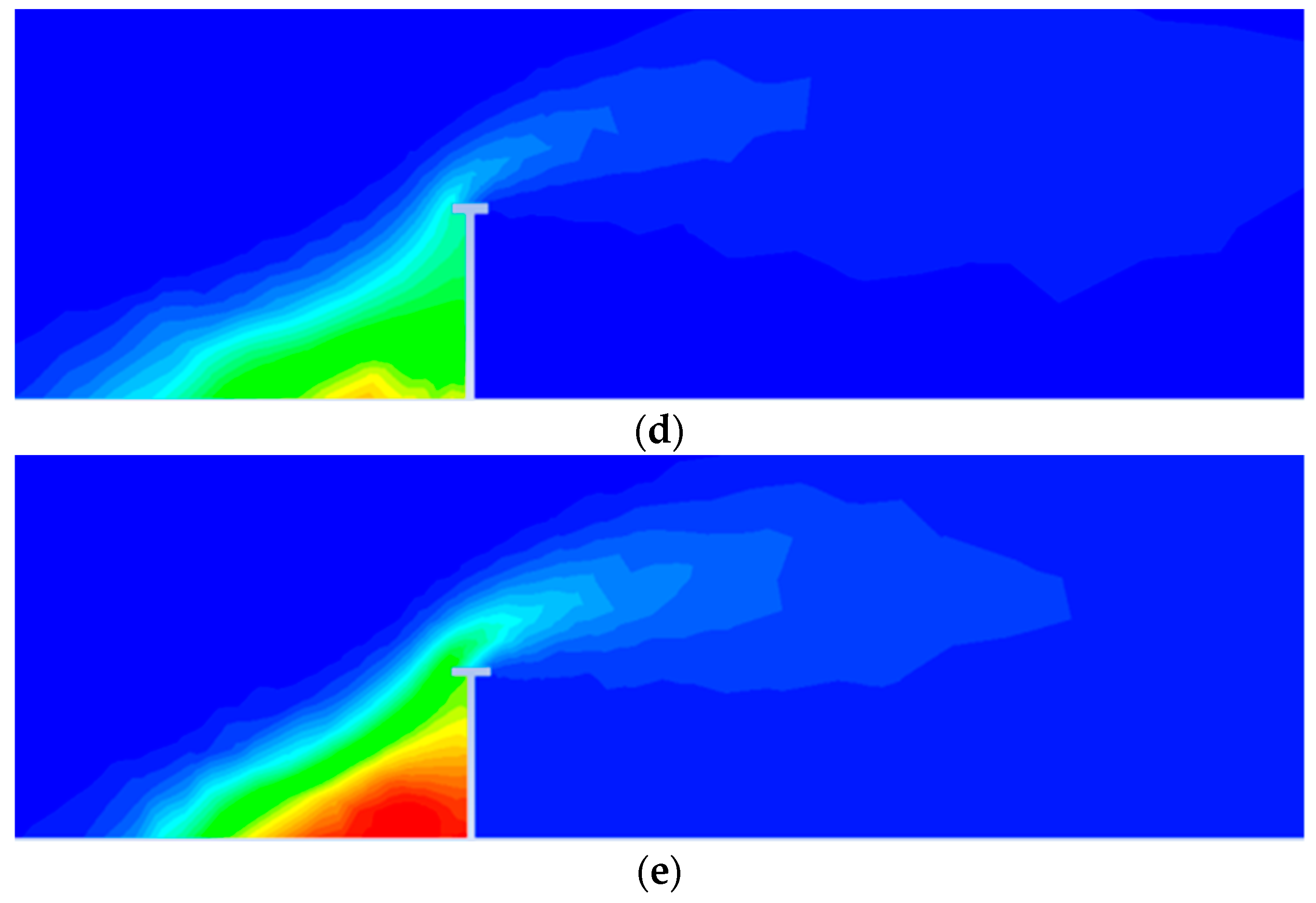
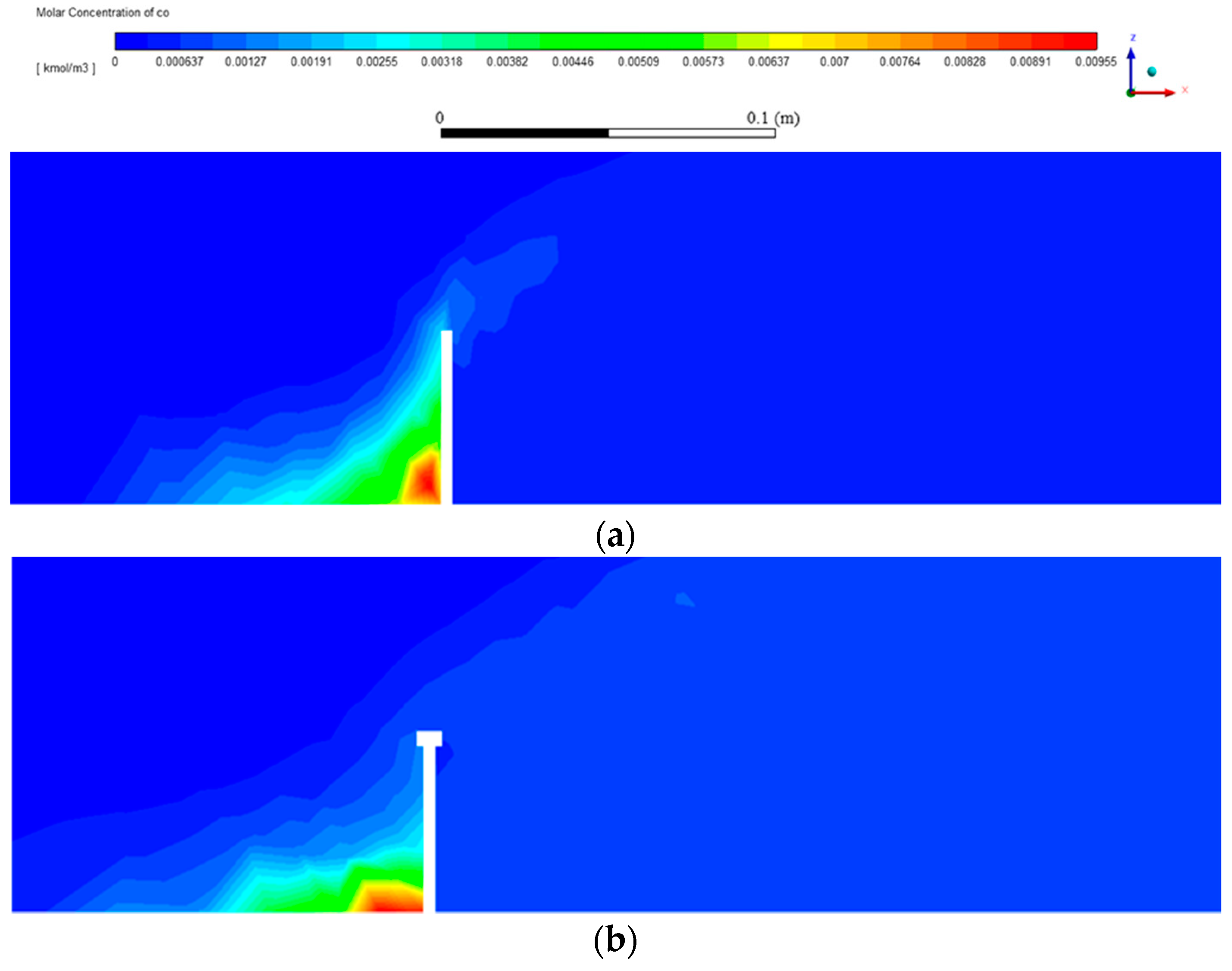
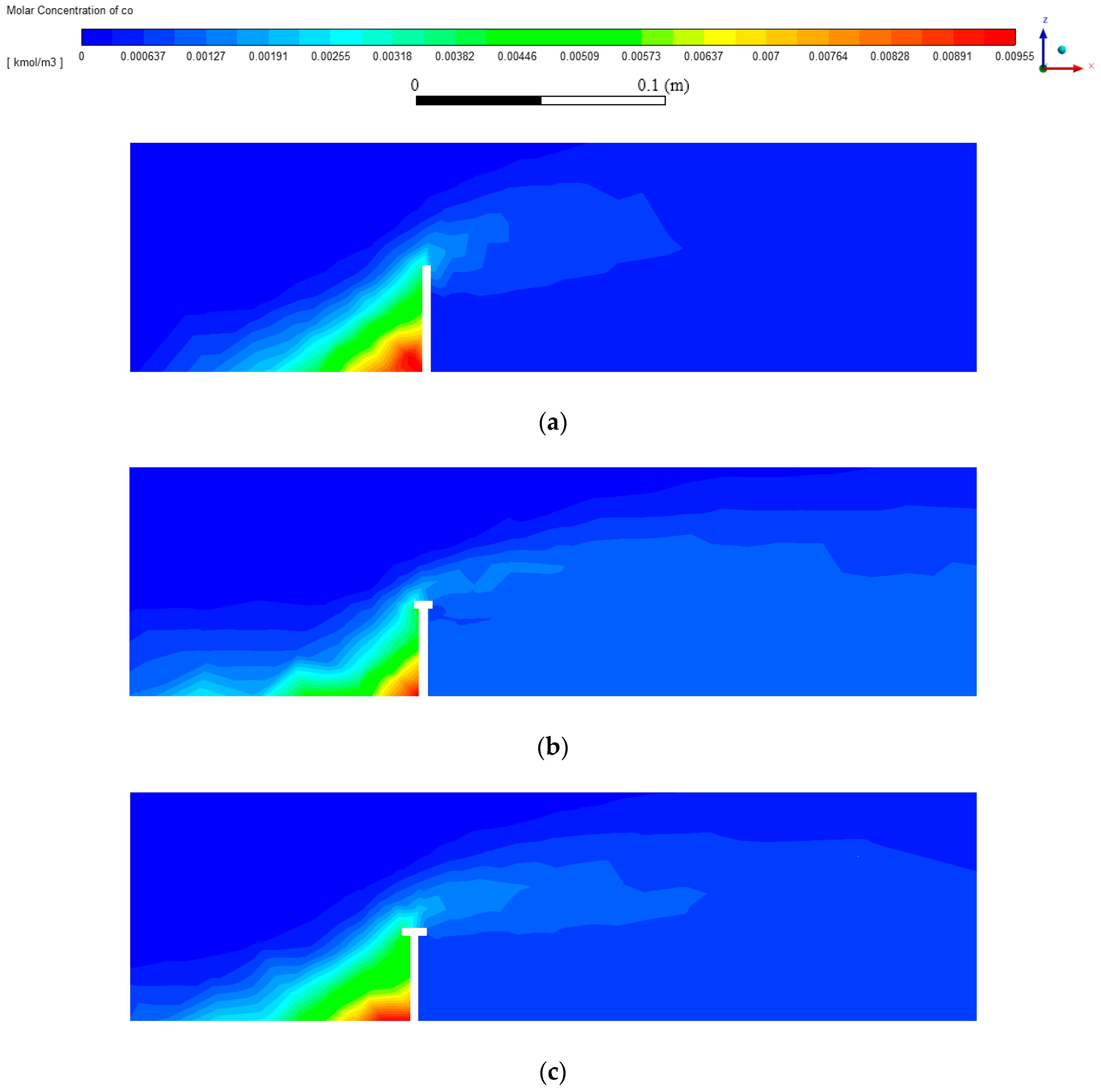
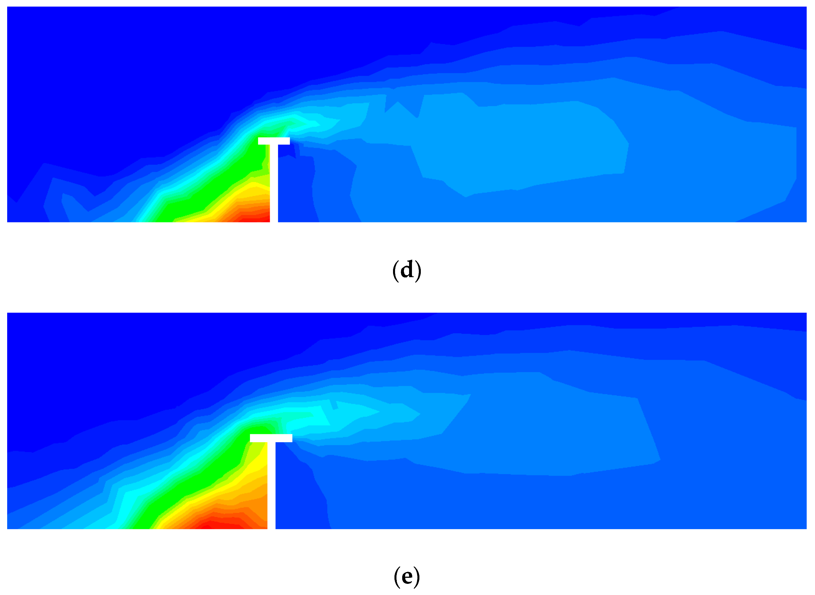
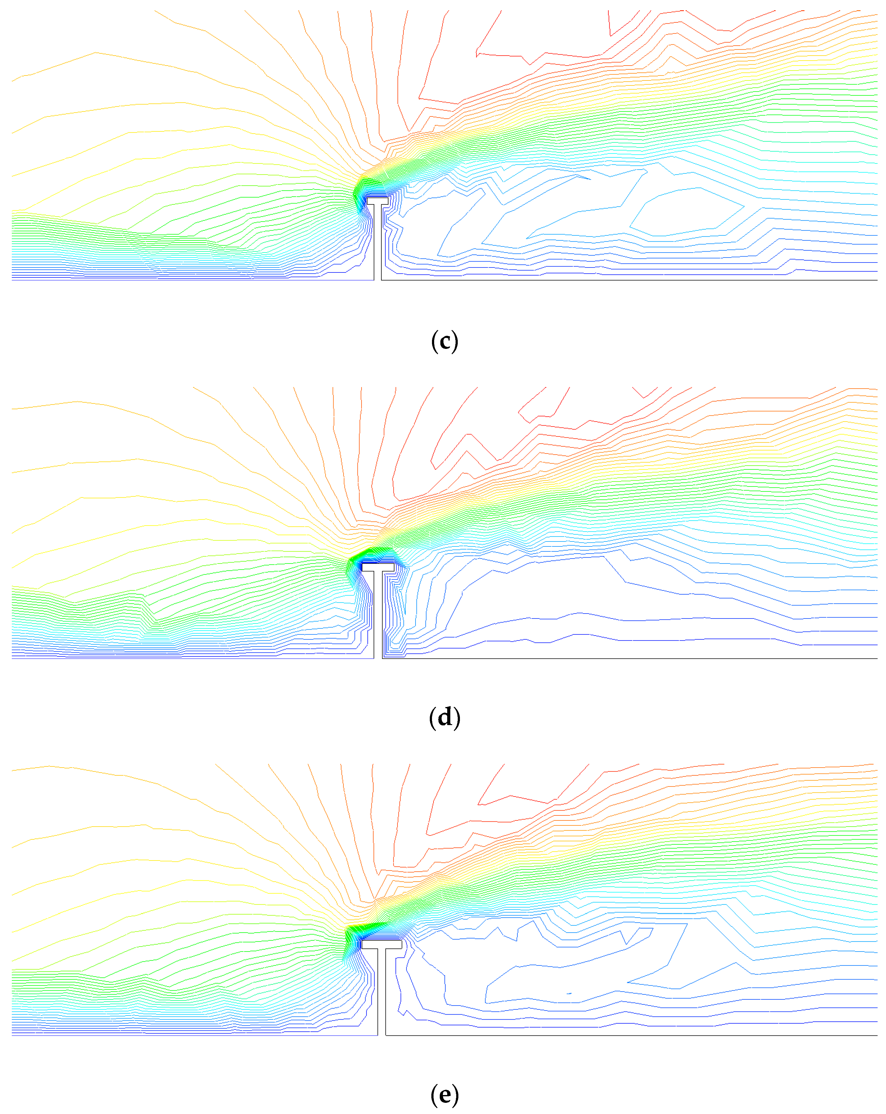
Table 1 were simulated by using realizable k-ε model and non-reaction species transport model. The results included contours and x-y plots of concentration distribution. To observe shape effects on emissions dispersion, a group of contours of molar concentration on the symmetry plane of the computational domain are shown below in
Figure 9.
As illustrated in
Figure 9, not all four types of the T-shaped noise barriers were able to significantly mitigate the downstream emission relative to the rectangular noise barrier. The performance was highly related to the noise barrier shape. T-shaped noise barriers with different top length had great differences. As expected, highway noise barriers could reduce the downstream emission concentration while much emission was trapped on the highway. The T-shaped noise barriers in cases 1, 2, and 3 had better performance than the rectangular and the T-shaped barrier in case 4 because they had less concentration both downstream and on the highway. However, case 4 suggested that a long top length for the T-shaped noise barrier didn’t have too much influence on the downstream emission compared to the base case. On the contrary, it gathered a little more concentration on the highway.
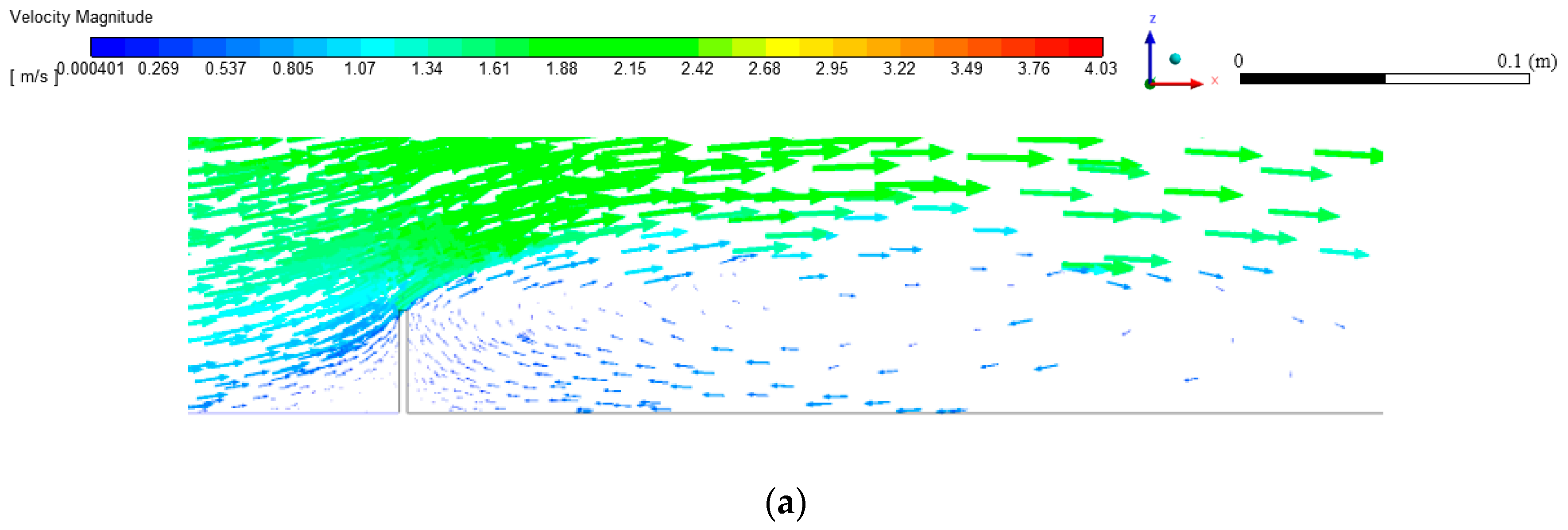
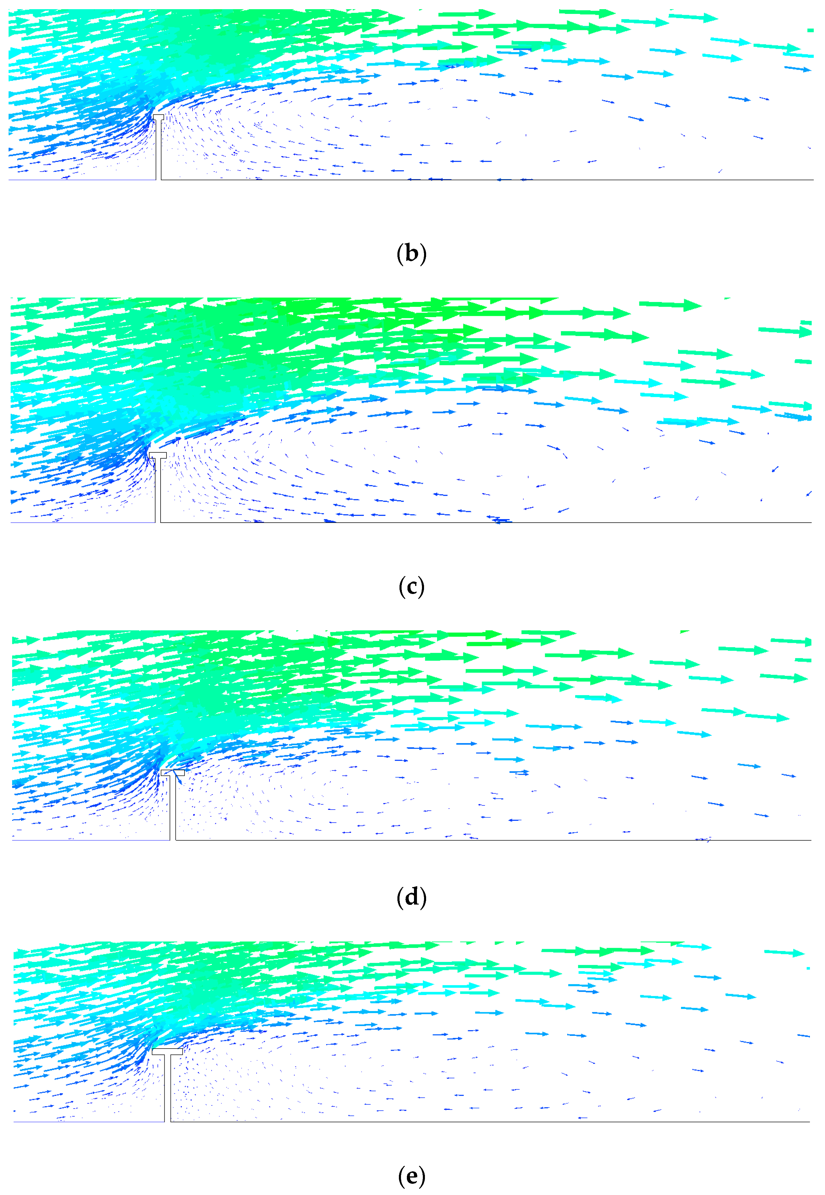
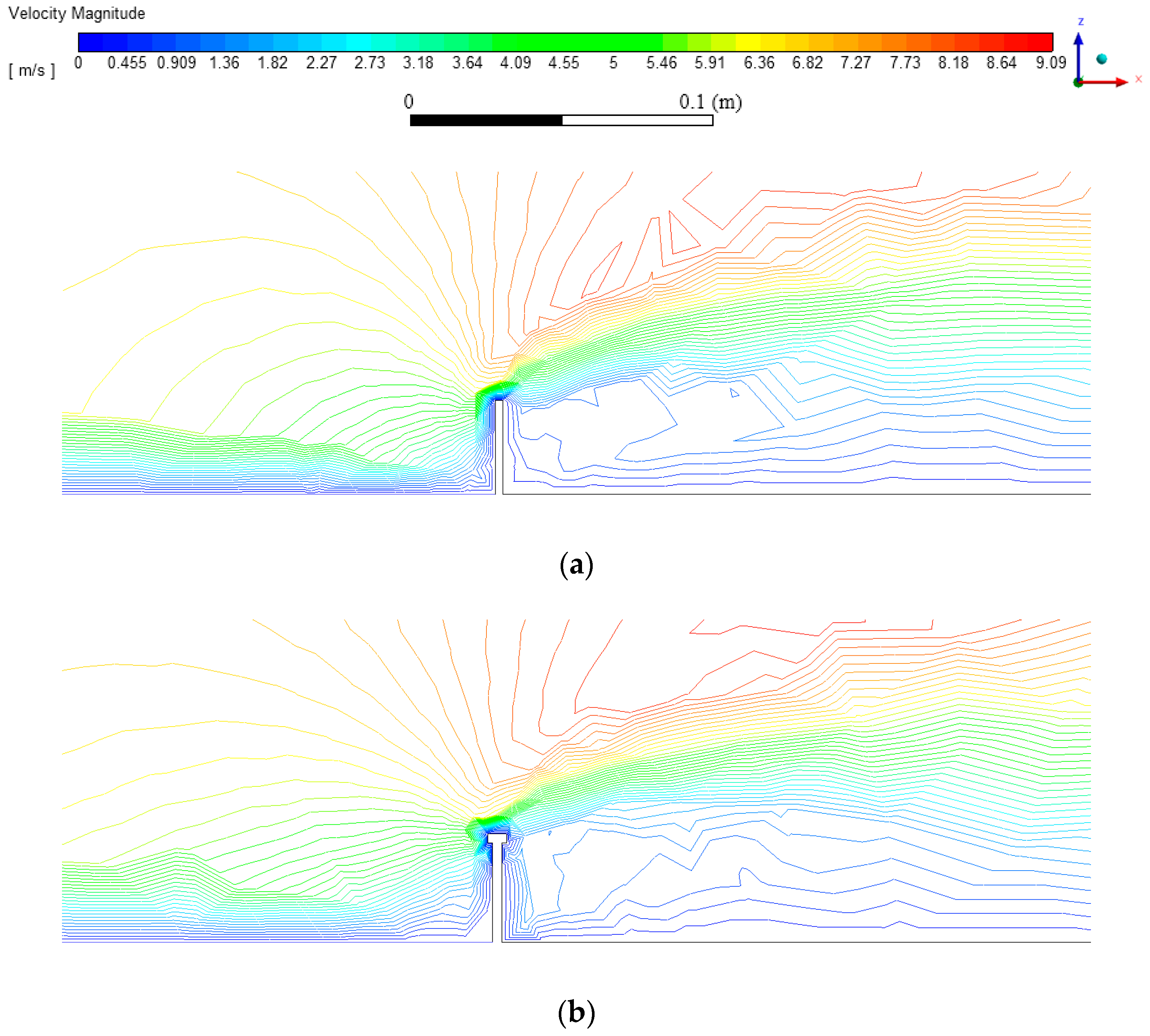
Next, wind velocity vector was obtained on the symmetry plane in
Figure 10. It shows the wind velocity vector near the noise barrier.
Figure 10 shows that wind climbed over the noise barrier and caused turbulence and vorticity behind the noise barrier. The turbulence behind the barrier can influence the downstream emission dispersion. Large turbulence intensity can increase mixing processes and contribute to the transportation and dissipation of automobile emissions. Also, it can be observed that the magnitude and direction of the wind velocity changed sharply near the top of the noise barrier, which was clear on the cross section of the barrier. That would create wind shear near the top of the wall, which can also influence the emission dispersion. Usually, there is also pressure difference in the area with big wind shear, which helps the emissions disperse. In front of the noise barrier, the incoming wind flow had to jump over the noise barrier so that the original low velocity met with high velocity. After passing the noise barrier, vortex has been generated. This flow pattern resulted in CO contours from which CO seemed to be dragged out in front of the noise barrier.
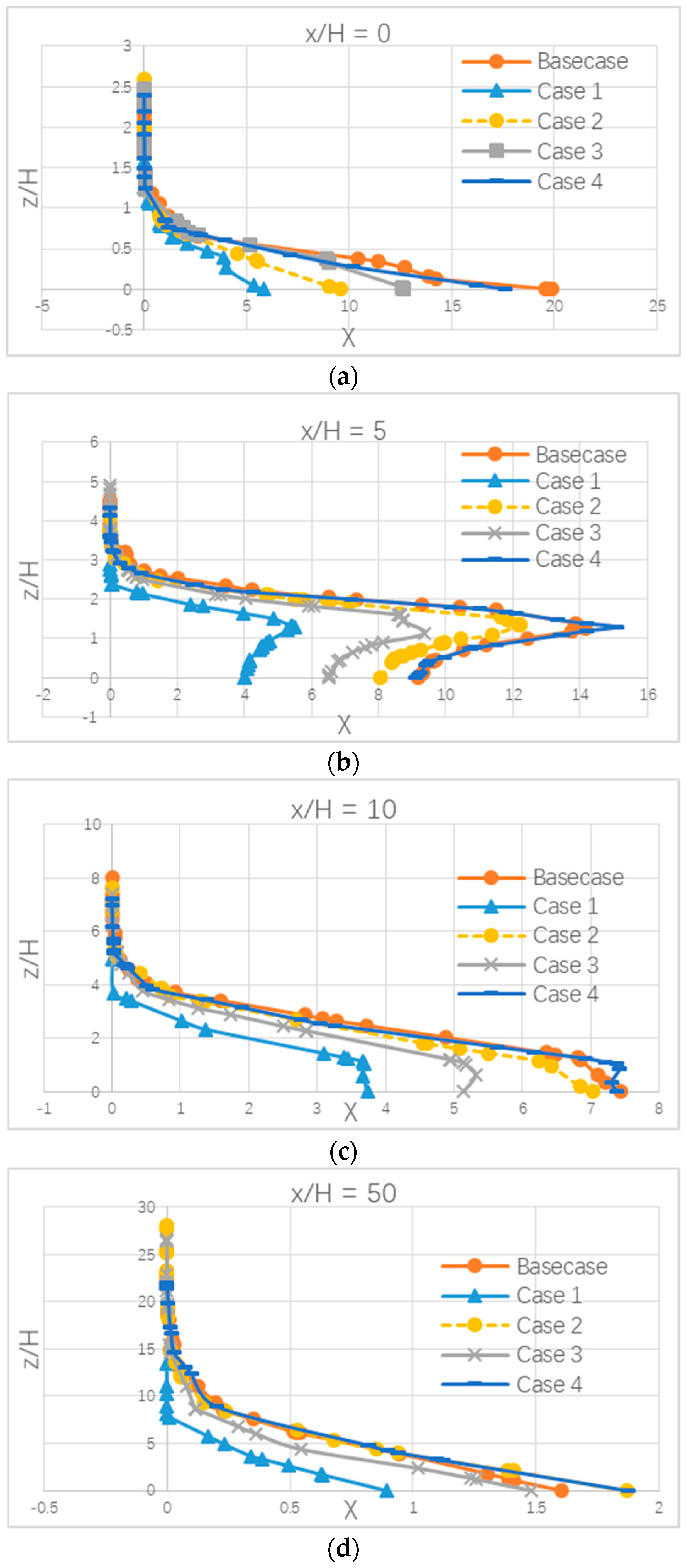
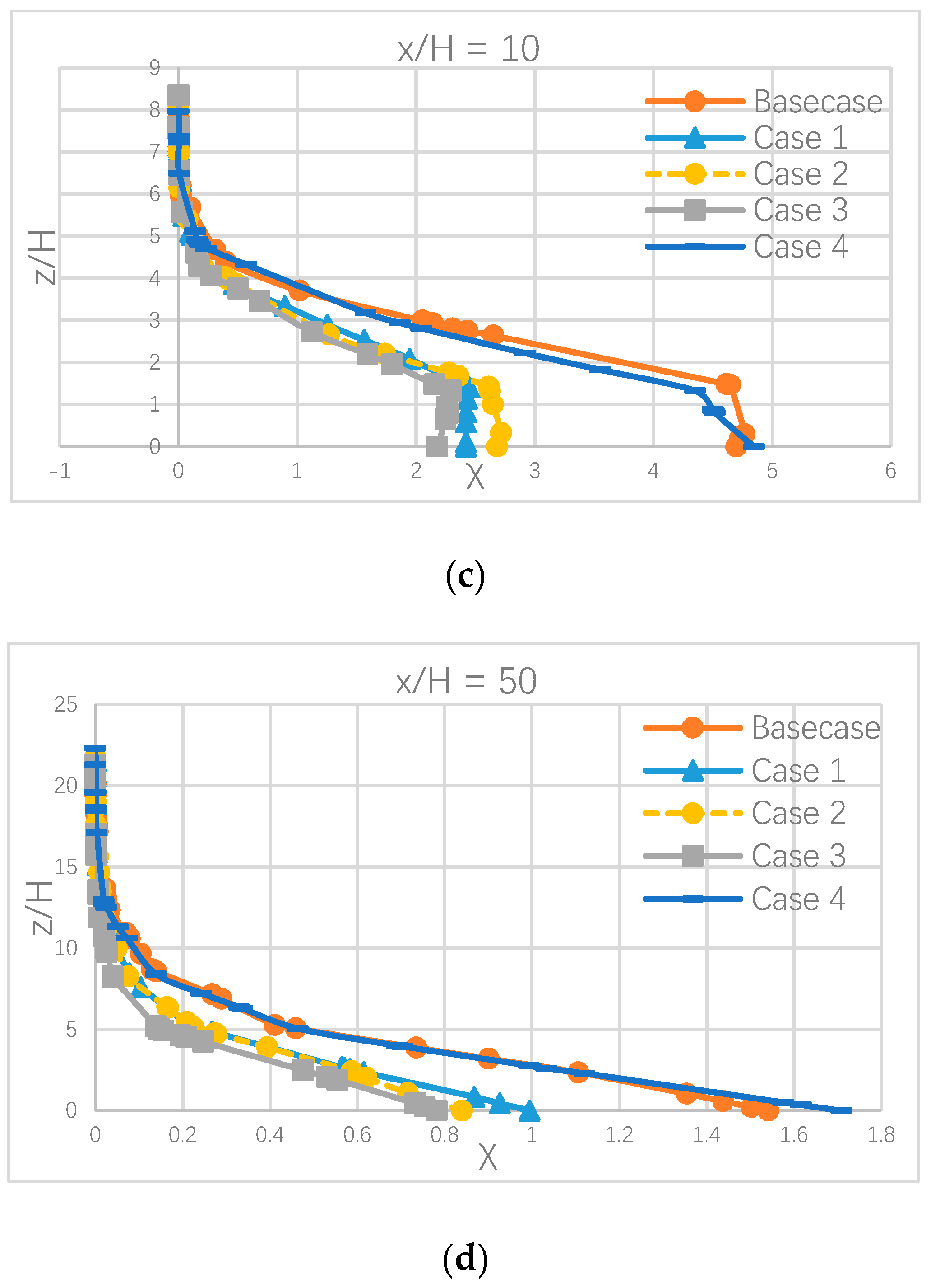
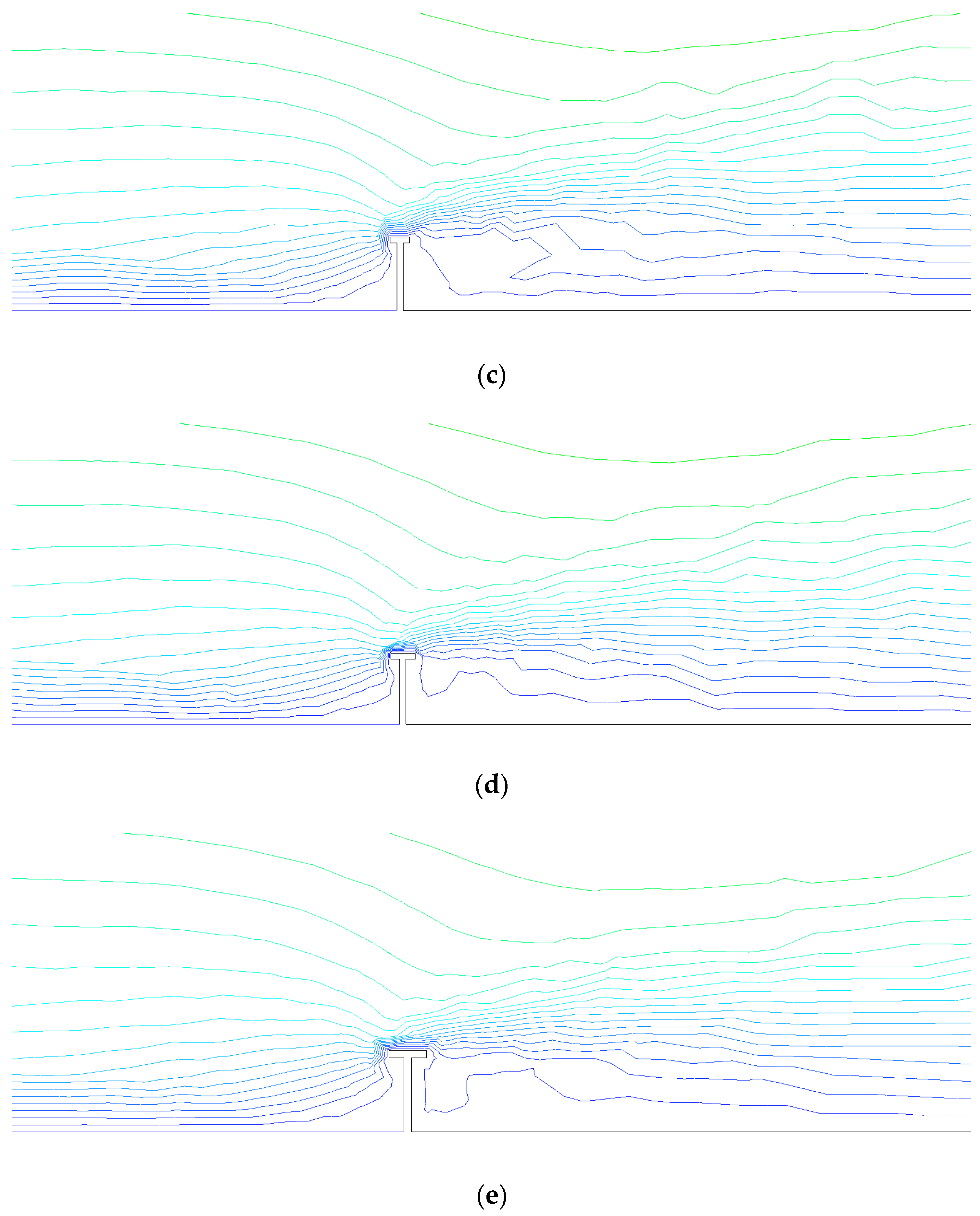
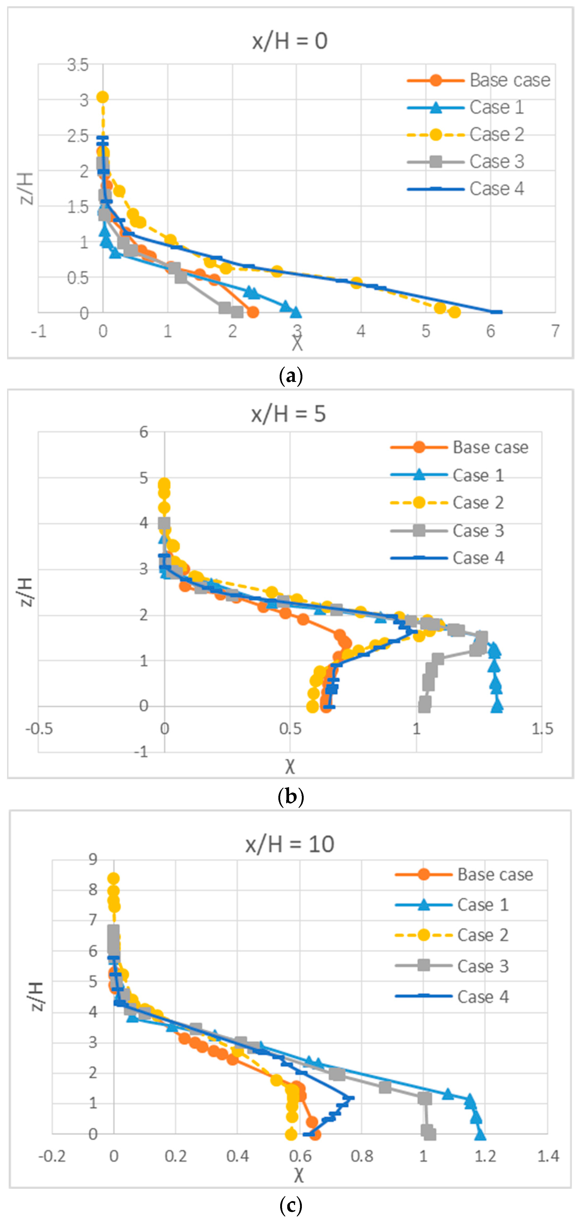
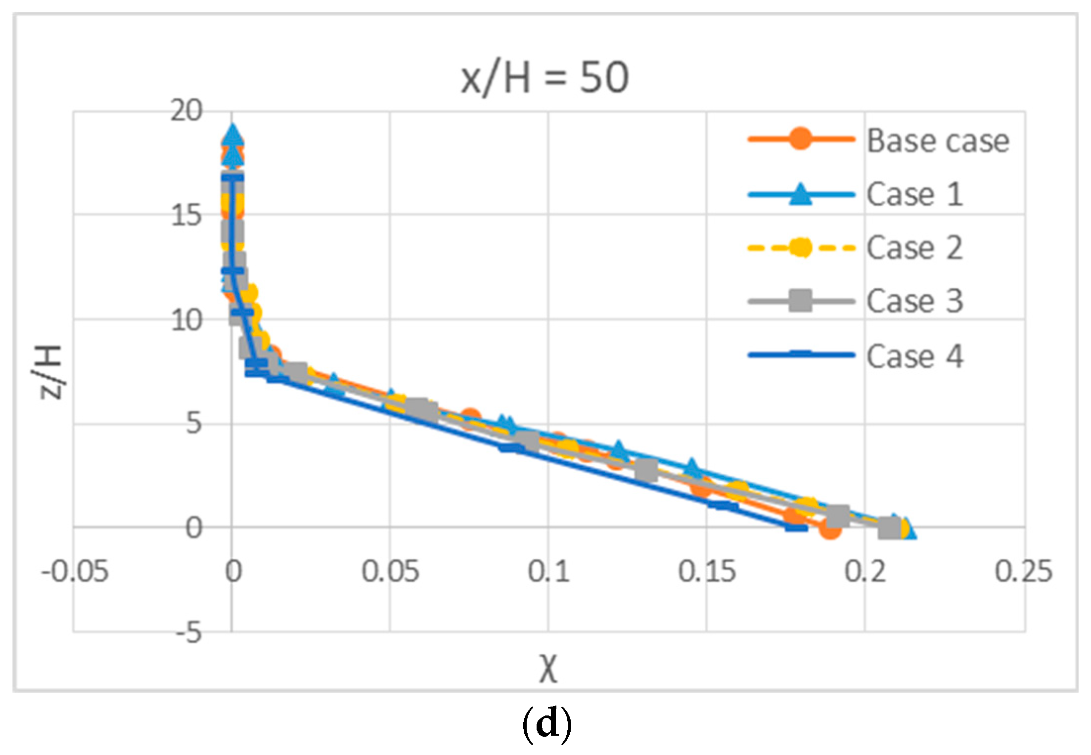
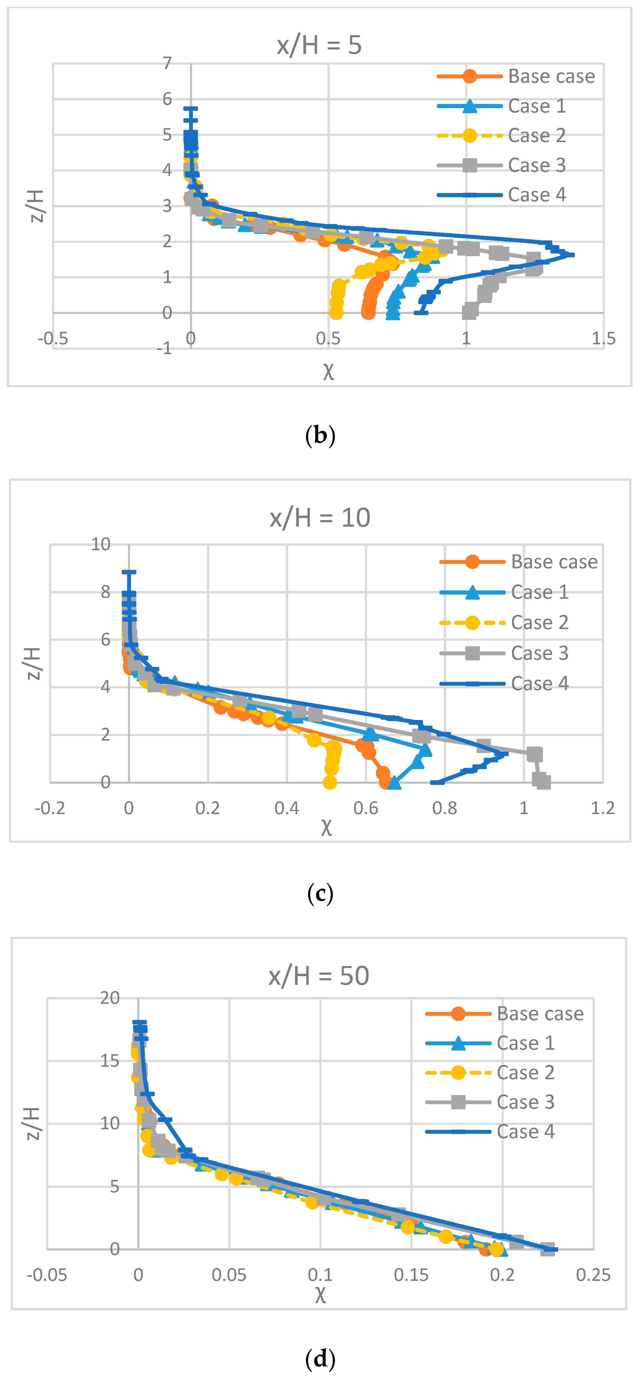
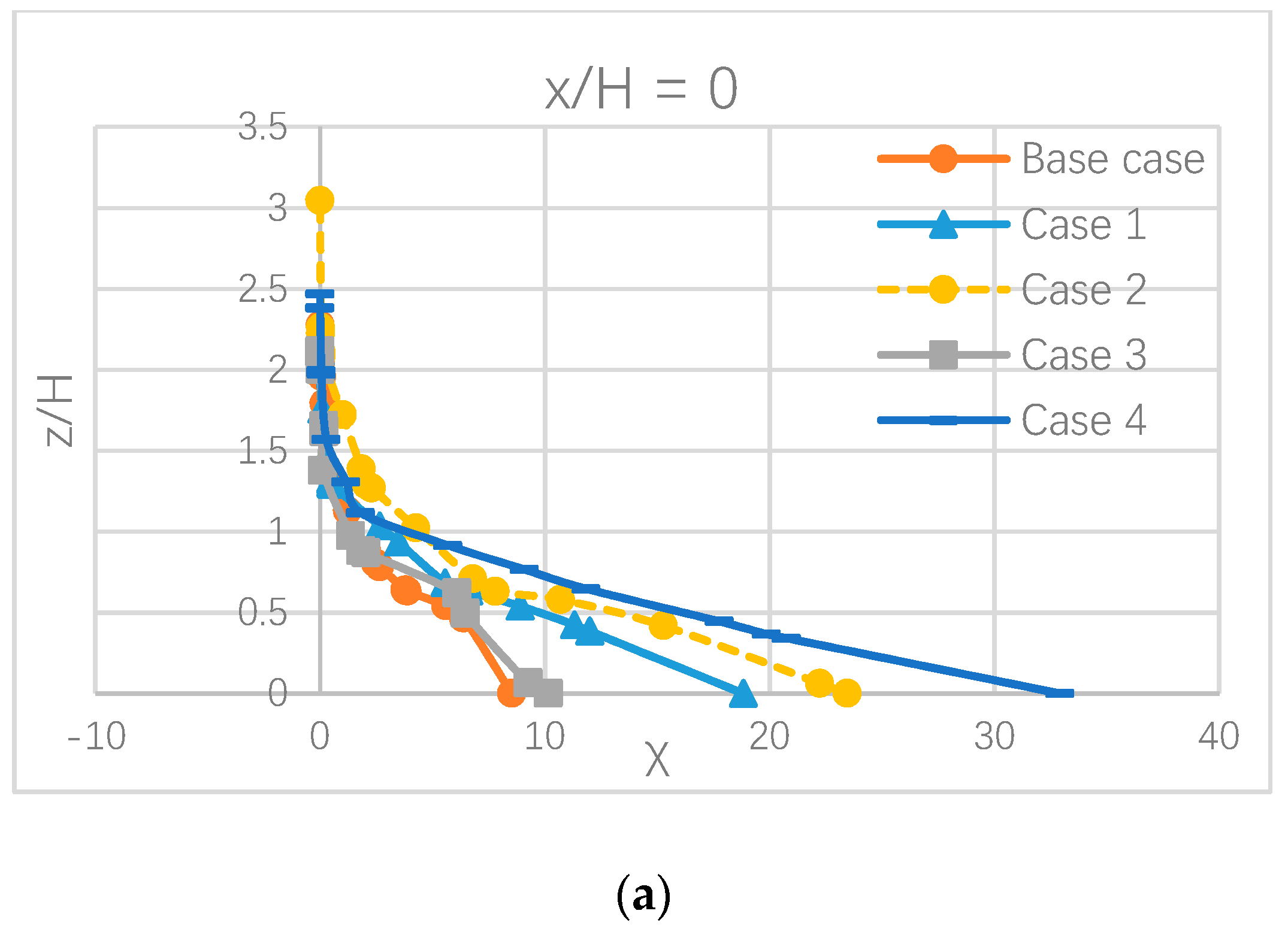
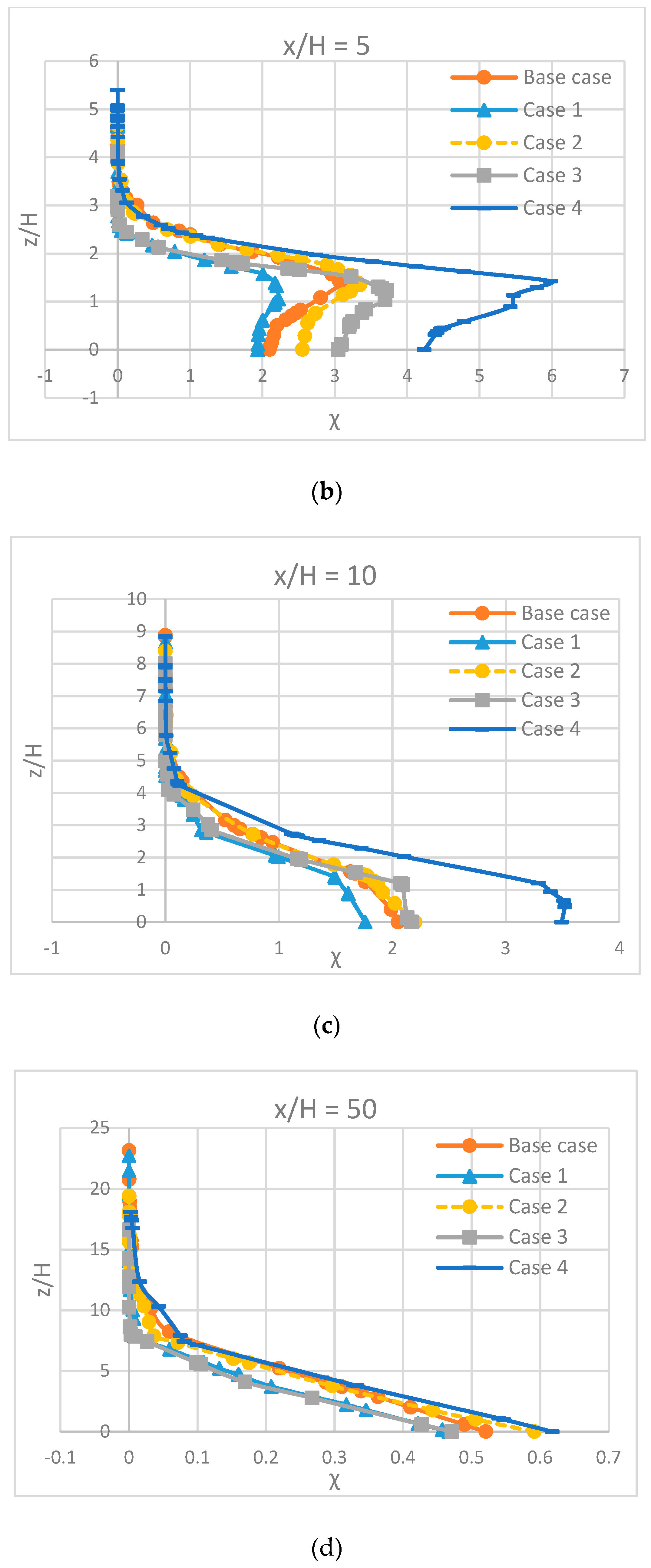
For clear comparison of the effects on pollutant dispersion from different noise barrier shapes, vertical distributions of normalized emissions concentration at four typical locations are depicted in
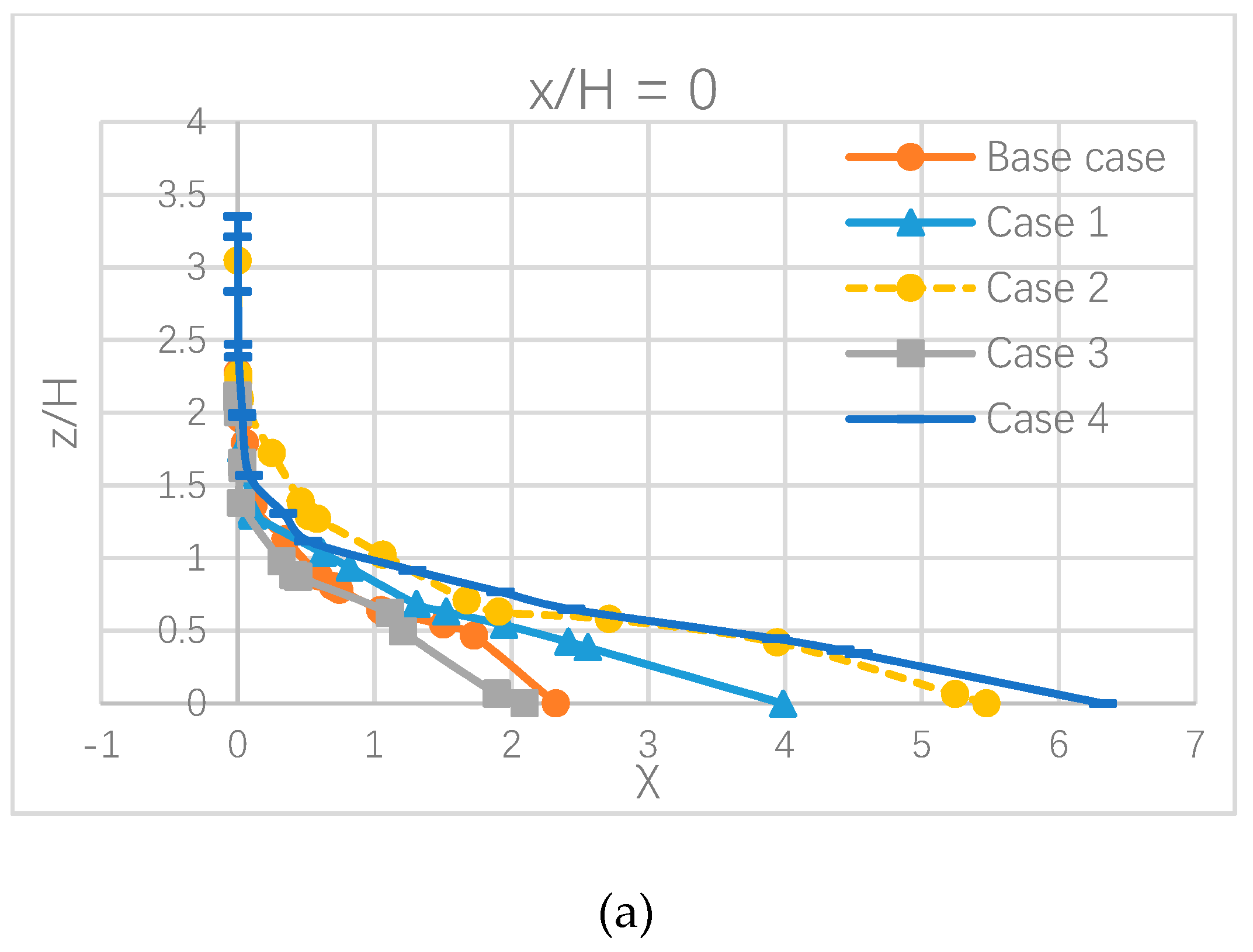
Figure 11. The horizontal axis is the normalized concentration χ. The vertical axis is the ratio of height to noise barrier height (z/H), which is also dimensionless. Each line recorded how much emissions from the ground (z = 0) to the height where the emission normalized concentration became zero.
The horizontal axis in
Figure 11 is the normalized concentration. The value of the normalized concentration decreased from the location x/H = 0 to 50. It implied that the emission was mostly on the highway and became less and less at regions further downstream. The vertical axis is the height. It was clearly demonstrated that the near-ground region always had more emissions than higher altitude regions.
The locations x/H = 5, 10 are areas relatively close to the highway. At these two locations, the base case and case 2 and 4 had similar vertical concentration distributions, but case 1 showed less concentration in the near-ground region. For the far downstream region, x/H = 50, all cases gave close results as the influence of noise barriers had less influence, although case 1 was able to mitigate more emissions.
All contours illustrated that noise barriers could reduce emissions concentration in the downstream area, but much of the emissions would be trapped on the highway, especially in the lower corner of the noise barrier. The further downstream the lower concentration in the near-ground region. For all four locations, case 1 appeared to have the best performance. Generally, T-shaped noise barriers can help reduce more emissions downstream than rectangular ones. However, a few of the T-shaped barriers had similar results while others varied slightly. The results highly depended on the top length of T-shaped barriers. Therefore, the further study was to increase the noise barrier height because the top length could not keep increasing while height remained the same.
In the following, all five cases with H = 0.06 m (9 m in the full scale) noise barrier were studied again. Different height, for T-shaped noise barriers, would change the ratio of the top length to the height, so it implicitly gave more available top lengths for the last simulation if the stability for the T-shaped structure had to be considered. Similarly, a group of contours and plots of concentration distribution were listed in
Figure 12 and
Figure 13.
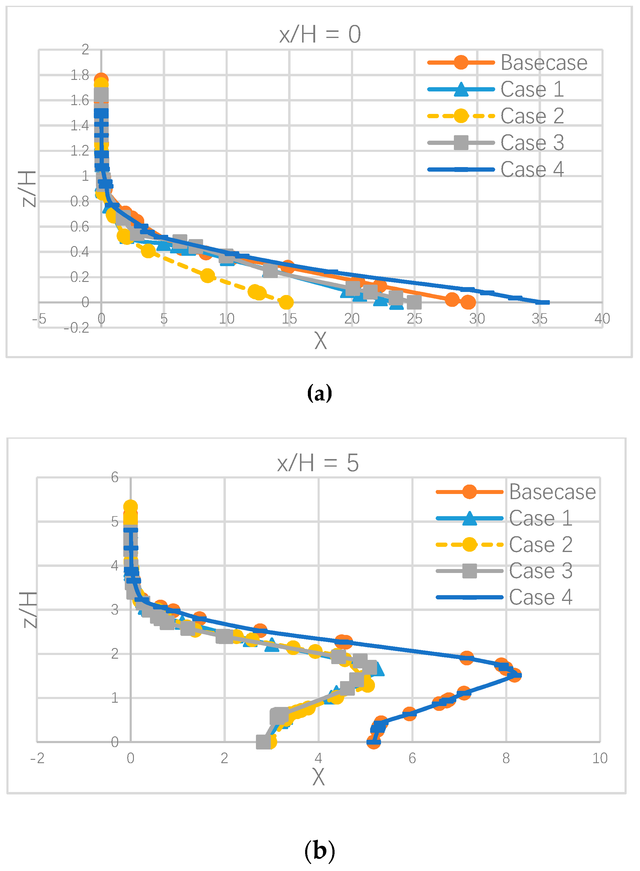
The contours in
Figure 12 show similar patterns to the previous simulation in
Figure 9. Different noise barrier shapes had different emission dispersions on the highway and in the downstream regions, and all followed the same trend. In
Figure 13a, case 2 had the best performance for the emission on the highway with the lowest pollutant concentration; in the downstream regions, from
Figure 13b–d, case 3 appeared to be the best one despite case 1 and 2 also performing relatively well. This could be explained by the fact that the top length would need to be accordingly longer if the T-shaped noise barrier had higher height, so that an optimized ratio of the top length to the height could be satisfied.
As a result, the best cases in this study were case 1 for 6 m high noise barrier and case 2 for 9 m high noise barrier on the highway, and case 3 for 9 m high noise barrier in the downstream region. For T-shaped noise barriers, an optimized ratio of the top length to the barrier height could range from 0.17 to 0.22.
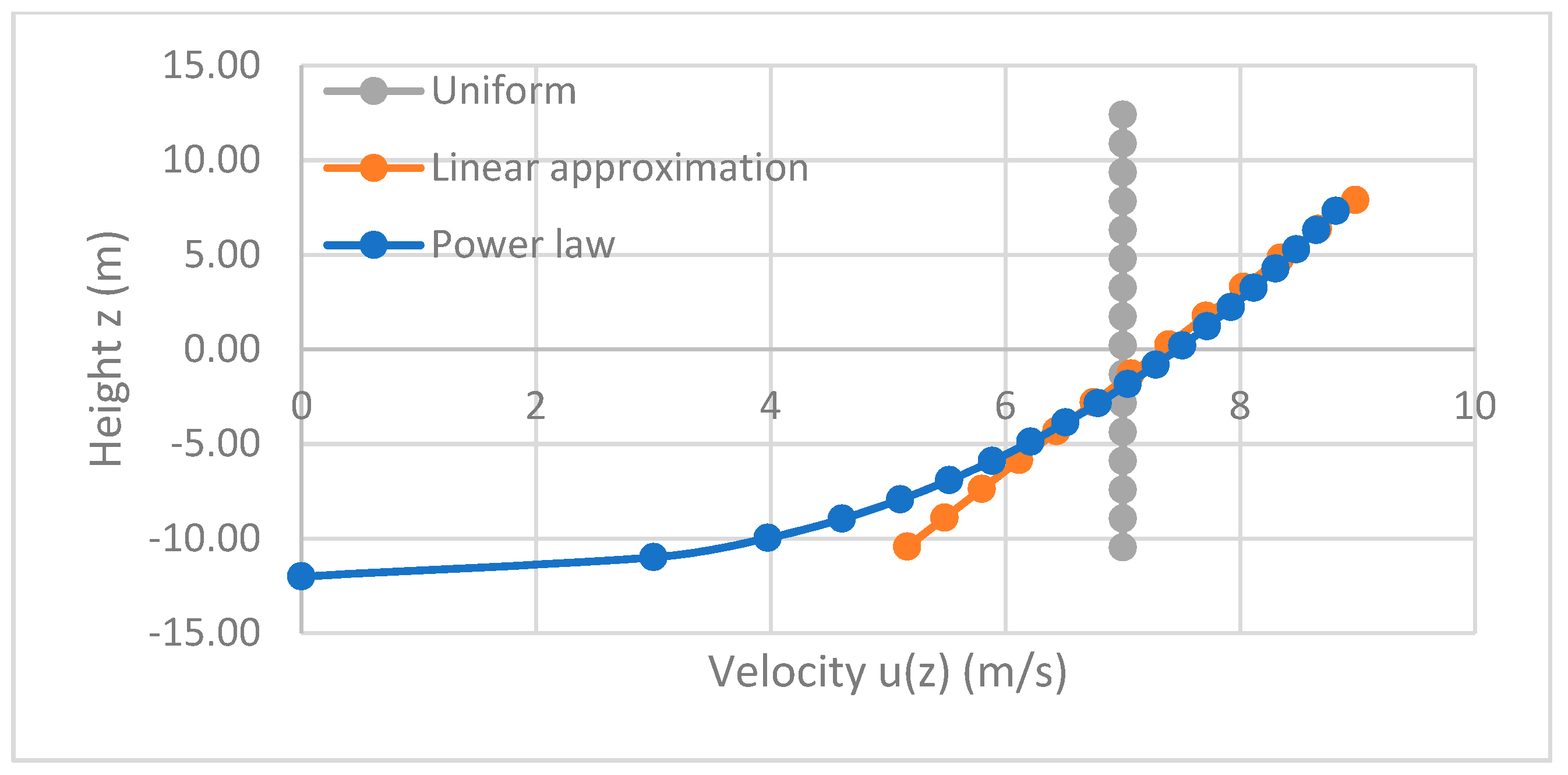
3.4. Influence of Inflow Conditions
The wind profile is usually described by the power law, but it could be considered using different inflow conditions in some special cases. One is the linear approximation to the power law. The other is the uniform inflow condition. The uniform inflow condition has a constant wind speed, so it does not have velocity difference and thereby no wind shear. The linear approximation describes that the wind speed has a linear correlation to the height, so it has constant wind shear. The power law describes that the wind speed varies with height exponentially, and the wind shear, along with big turbulence and vorticity, varies with height. The three inflow conditions are shown in
Figure 14. The height was offset to the height of wind turbines from the sea level, which was 12.2 m [
17].
3.4.1. Uniform Inflow
Uniform inflow is a case in which the wind velocity is constant at 7 m/s [
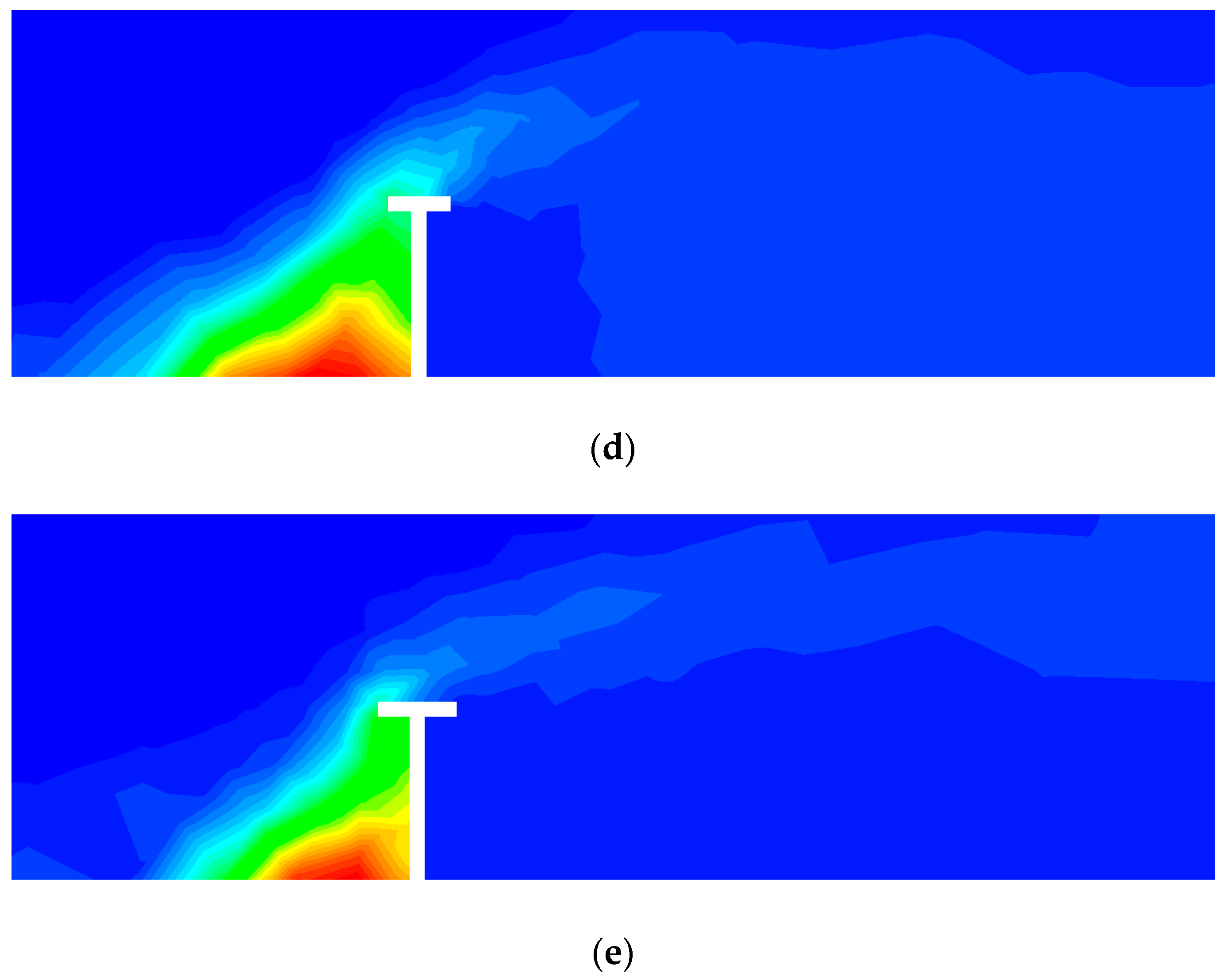
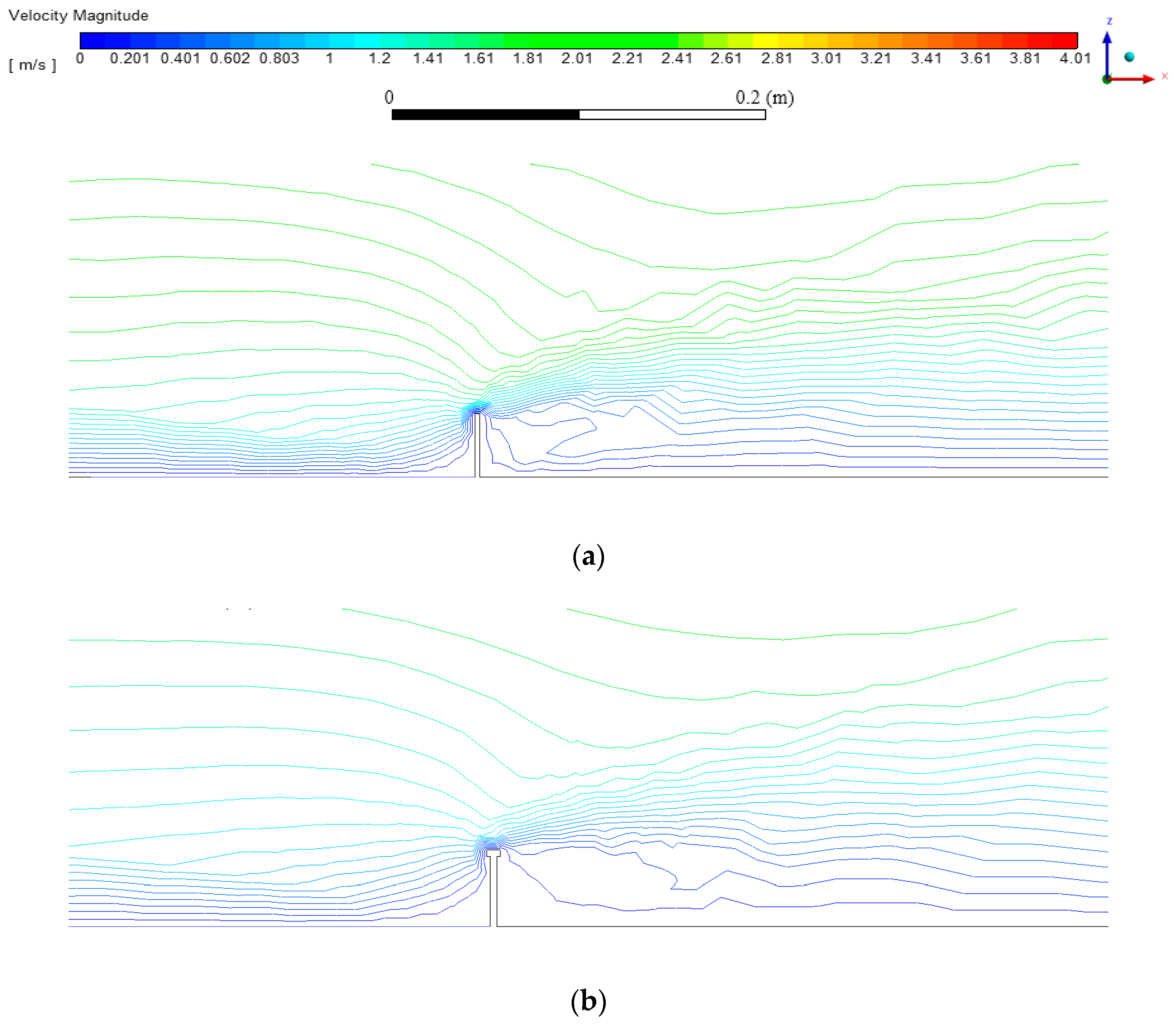
17]. Simulation cases with 0.04 m high (6 m in the full scale) noise barriers were solved with the uniform inflow condition. The contours of CO molar concentration and velocity streamlines are shown in
Figure 15 and
Figure 16.
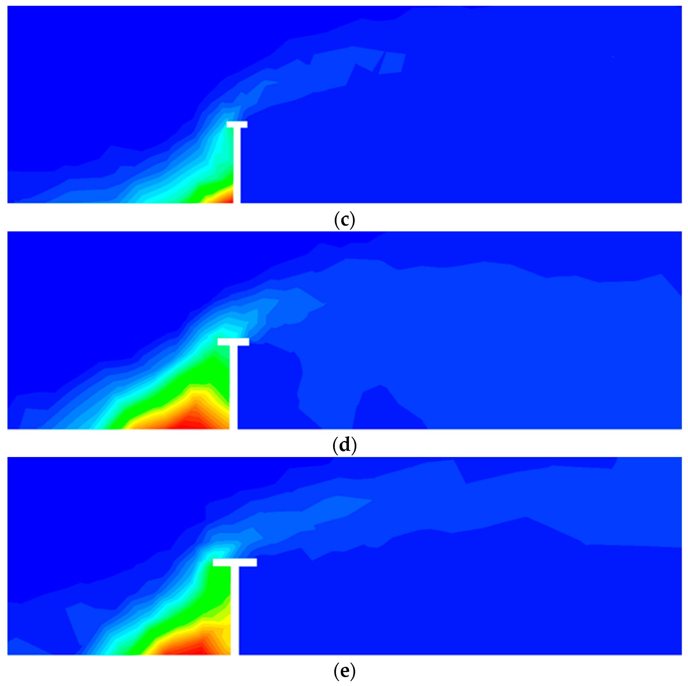
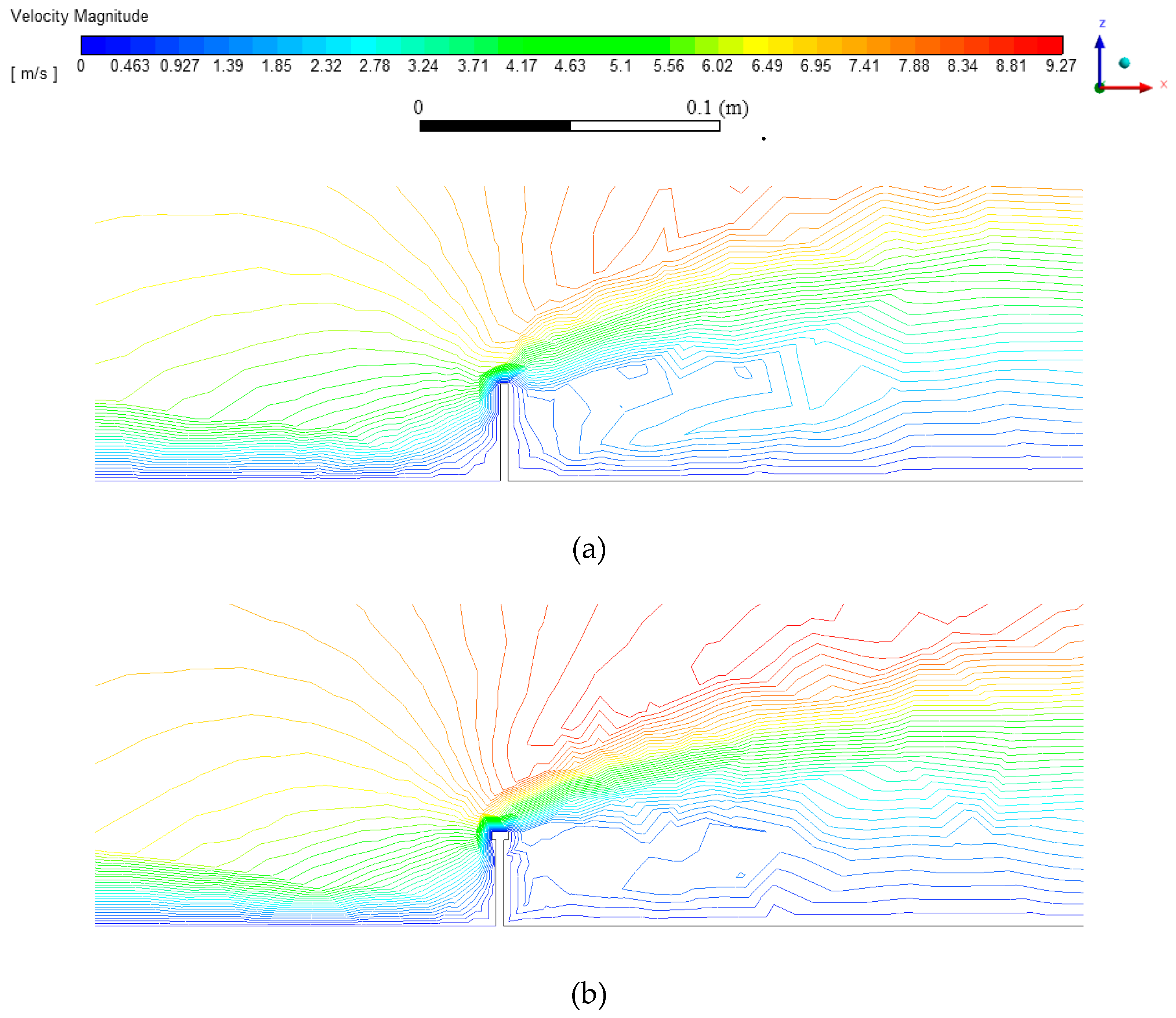
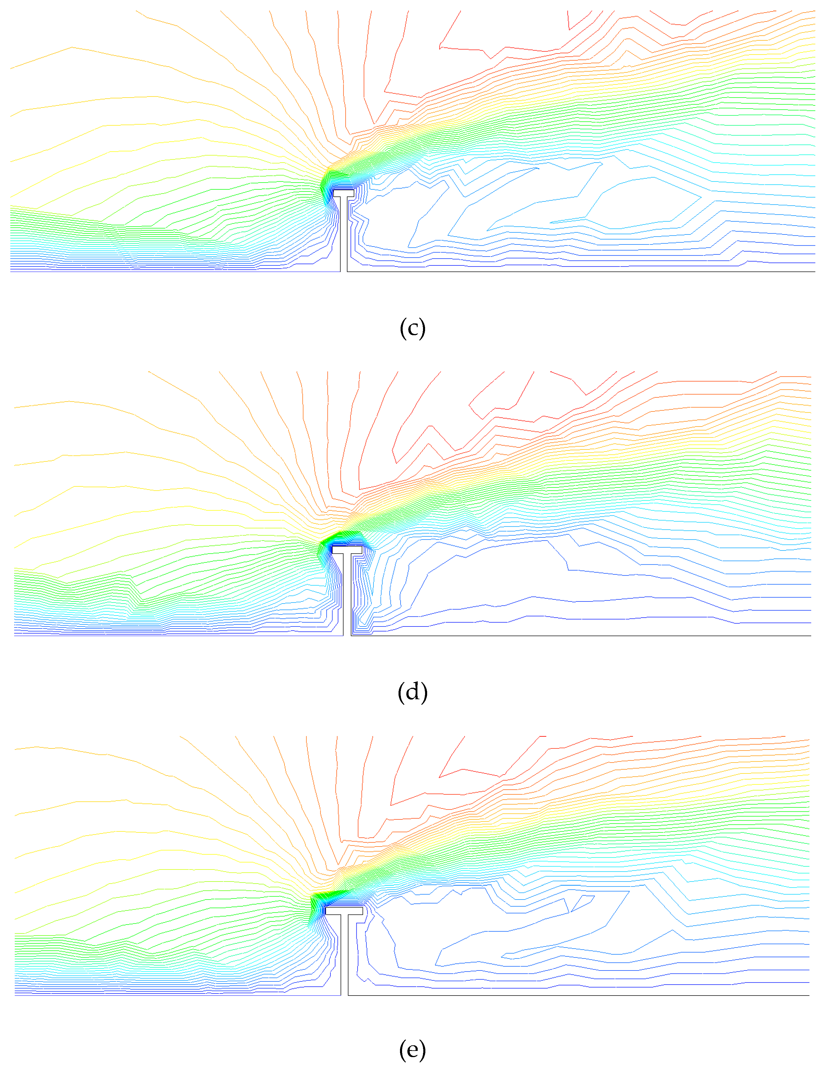
CO concentration contours could show the emission dispersion directly and intuitively. Velocity streamlines could imply the wind shear. As mentioned before, the uniform inflow would not create wind shear, so the turbulence caused by incoming wind barely exists. However, one can tell from
Figure 16 that the streamline became very dense on the top of the noise barrier, which means wind shear appeared on the top of the noise barriers, due to the change of flow cross sessional area. Noise barriers could create turbulence around themselves. The noise barrier shape influences the turbulence and thereby the emission dispersion. The base case appeared to have denser streamlines near the noise barrier, so the T-shaped noise barrier may not perform better at reducing emissions downstream. Consequently, vertical distribution of CO at four locations was obtained again and is shown in
Figure 17.
Under the uniform inflow condition, base case, case 1 and 3 appeared to have similar performance on the highway; meanwhile, case 2 and 4 also had similar results. In the near-highway regions, base case, case 2 and 4 turned out to be similar cases and became relatively better cases under the uniform inflow condition. In the far downstream area, the CO concentration would become very light, so there was not a big difference between each case. As a matter of fact, the shape effects of the noise barrier would become insignificant in the far downstream area.
3.4.2. Linear Approximation
The linear inflow condition approximates the power law. The equation for the linear approximation is adopted as [
17]:
From the equation one can tell that the wind velocity is linear to the height. At zero height, it reaches the same wind speed as the uniform inflow, 7 m/s. Simulation results of linear approximation are shown in
Figure 18,
Figure 19 and
Figure 20.
Under linear inflow condition, unlike the uniform inflow condition, the results of five cases varied a lot in the near-highway regions in
Figure 20b,c. That could be explained with the existence of wind shear.
Figure 19 suggests that velocity streamlines under linear inflow condition had larger differences than those under uniform inflow condition. Linear inflow would create wind shear that could contribute to the transportation and dissipation of highway emissions. Consequently, the emission distribution downstream near noise barriers would be greatly decreased compared to the uniform inflow. Case 3 showed the least concentration on the highway (x/H = 0), while case 2 was in a better condition for near-highway regions (x/H = 5, 10). However, the level of emission reduction by the T-shaped noise barrier was not critical compared to the base case results. Likewise, all cases had very similar results in the far downstream area (x/H = 50) because the shape effects of noise barrier became insignificant.
3.4.3. Power Law
By using the power law parameters in the reference [
17], the reference height was 10 m, and the reference velocity was 7 m/s. The exponent of the power law was 0.35. The power law can be described as:
The wind velocity varies with height exponentially. The wind speed has the same magnitude as the uniform inflow at zero height. The results under the power law profile are shown in
Figure 21,
Figure 22 and
Figure 23.
The velocity streamlines under the power law inlet condition were similar with those under the linear inflow condition, because both power law and linear inflow could create the wind shear and because the linear inflow is originally an approximation of the power law. As a result,
Figure 22 shows that the great change of the wind velocity, i.e., the wind shear, was still present under the power law profile. Hence, the emissions dispersion would be further influenced. The results were embodied in the CO concentration contours and plots. For the near-highway regions, case 1 was still the best under power law even though the reference velocity and height were different for this simulation. However, it was unable to have dramatic reduction on CO concentration, especially in the far downstream area where case 1 already had similar results to case 3.
4. Discussion
In this research, ANSYS®Fluent 19.2 (Ansys Inc., Canonsburg, PA, USA) was applied to simulate the noise barrier shape and different inflow wind shear condition effects on highway automobiles emission dispersion. Validation was first conducted for various RANS turbulence models. By comparing with different turbulence models, the realizable k-ε model coupled with a non-reacting species transport model was selected due to its best match with experimental data.
Numerical simulation results of highway emissions dispersion were obtained with rectangular and T-shaped highway noise barriers. The contours of CO dispersion and the vertical distribution at four typical locations were investigated. Results suggested that T-shaped noise barriers can help to improve the air quality in downstream areas, showing better effects than rectangular noise barriers. The level of emission reduction was dependent on the top length and height of T-shaped barriers. In other words, the ratio of the top length to the height was a critical parameter.
The shape effects of highway noise barriers on the vehicle emission dispersion were not significant at the location of the highway and far downstream regions because much of the emissions were trapped on the highway, and the emissions were already reduced in far downstream areas. However, the emission dispersion varied with noise barrier shapes in near-highway regions; for example, 10 times noise barrier height far downstream region, T-shaped noise barriers could have better performance on reducing the emission concentration downstream than rectangular ones. It was suggested that the ratio of the top length to the height determined the performance of T-shaped noise barriers. The optimized ratio is around 0.2.
The wind velocity vector and streamline could be used to explain the noise barrier shape effects on highway vehicles emission dispersion. When the wind passed across a noise barrier, the biggest wind velocity difference was on the top of the noise barrier, so there would be wind shear that causes turbulence; then the turbulence could influence the emission dispersion downstream. In addition, optimized T-shaped noise barriers would also create back flow that could further reduce the emission concentration downstream.
The noise barrier shape effects were highly dependent on the inflow conditions. After the wind passed the noise barriers, it could continue to swirl behind the noise barriers, depending on the way the wind travelled. The swirls corresponded to the shapes of the noise barriers, influencing emissions dispersion downstream. Different inflow conditions create different wind shear and turbulence. The uniform inflow did not have wind shear, but the linear inflow and the power law inflow did. As a result, the best case under the power law would not necessarily be the best one under linear or uniform inflow conditions. The combination of wind speed, wind shear and turbulence intensity influence the highway automobiles emission dispersion.
In summary, T-shaped noise barriers would have better performance not only on noise reduction but also on automobile emissions reduction if an optimized ratio is satisfied. In far downstream areas, automobile emissions concentration has already been reduced, so the shape effects of noise barriers are insignificant. Moreover, the magnitude of reducing automobile emissions near highways could be influenced by inflow conditions. The T-shaped effects would stand out if inflow conditions could create wind shear. This paper focuses on the noise barrier shape effects on highway vehicle emission dispersion under neutral atmospheric conditions. Future research can be conducted with the combination of different thermal condition effects as well as considering the effects from moving vehicle induced wake flow on emission dispersion for more realistic and accurate results.


