1. Introduction
Maladaptive vessel wall remodeling can occur when pressure and shear forces are altered at the blood vessel wall. For example, vessel wall remodeling is known to occur as a result of changes to ascending aorta blood flow in the presence of aortic valve diseases, which generally change valve stiffness and affect its ability to open. These changes to aortic hemodynamics will alter the hemodynamic forces at the ascending aortic wall. If the magnitude of these forces exceeds their normal physiologic range, extracellular matrix remodeling, abnormal protein expression, and ultimately aortopathy, in the form of vessel dilation or dissection, may occur. For these reasons, diseases of the aortic valve, such as those associated with regurgitation and stenosis, are often linked to aortopathy [
1,
2,
3,
4,
5]. A detailed review of the development of calcification with narrowing of the aortic valve opening and reduced blood flow to the body was presented in [
4,
6]. Similar negative effects may occur when an implanted prosthetic valve leads to hemodynamic parameters outside of the range in healthy people. With that in mind, numerous studies attempted to establish a relationship between altered transvalvular hemodynamics and patient risk for catastrophic events (such as aortic dissection) [
7].
The deformation of the leaflets of the aortic valve is driven by a coupled interaction between tissue and blood, leading to a complex fluid–structure interaction (FSI) problem that ultimately determines the overall hemodynamic environment in the ascending aorta [
3,
8,
9]. As opposed to the development presented in [
9], where the bending of the valve was completely neglected, this work includes bending stiffness in the modeling of the aortic valves. The importance of bending stiffness in the analysis of heart valves has been recognized in the past [
10,
11], and its inclusion requires a shell model, flexible enough to incorporate varying thickness of the valve and its varying properties. This appears to be particularly important in the case of diseased valves, as its apparent thickness and material properties are likely to increase the valve’s bending properties significantly. Various mathematical models of the leaflets (and of aorta) can be employed in the analytic or numerical solution of the problem to describe their behavior. The major challenge for this endeavor is the determination of their real material and geometric characterization, knowledge of which is scant in the literature. For example, in the presence of the most common form of aortic valve disease, calcific aortic valve stenosis, the deformation properties of the valve leaflets and their mass are altered, as calcified nodules develop on the valve leaflets, causing the leaflets to stiffen (valve sclerosis), thus preventing a complete opening of the valve. This process, while highly variable and difficult to quantify, is very important, as the resulting obstruction of blood flow increases ventricular afterload and creates high velocity, eccentric jets downstream from the obstructed valve [
12]. Some methodologies to tackle these difficulties were recently described in [
13], where the three-dimensional geometry of the valve calcification mimicked observed patterns. However, that was combined with a very simplified, cylindrical shape of aorta, which should prevent the observed hemodynamic flow pattern, such as helical blood flow. Interestingly, the numerical results presented in [
13] compared quite well with those seen in clinical observations. In this work, the realistic shape of aorta is used, and its supra-aortic branches are included (brachiocephalic and left subclavian arteries).
The association between abnormal hemodynamics and the diseases it causes is established by medical exams of people whose blood flow has been altered for a sufficiently long time to cause significant maladaptive remodeling and the appearance of symptoms signaling a problem. Although unfortunate, the observations of the anomalies in real people constitute an important aspect of developing medical knowledge, necessary to devise appropriate remedies. However, when the association between those anomalies and hemodynamics is already known (and, as alluded to below, the medical community is presently aware of such associations), an equally important aspect is early prognosis if some specific changes in the properties or geometry of the heart valve (caused, for example, by disease of the natural valve or by the selected design of a prosthetic valve) result in blood flow that is likely to trigger other future complications. To predict that, relatively detailed information about the corresponding hemodynamics needs to be known, and that, arguably, is best extracted through simulations, provided that sufficiently realistic models are adopted. Simulations can be of great value both in designing a remedy for a malfunctioning natural valve and in optimizing the design of a prosthetic valve. They permit relatively easy modifications of the model and analysis of many pertinent scenarios, related, e.g., to contemplated surgical interventions or to various options of prosthetic valve design. They also allow examining any desired detail of the resulting hemodynamic state with a high degree of fidelity [
3].
An important reason for engaging simulations in predicting possible negative consequences of abnormal hemodynamics is the level of detailed information they can provide. For example, low and oscillating wall shear stress (WSS) fields have been shown by MRI observations to be associated with abdominal aortic aneurysm growth, but high WSS has been associated with abnormal ascending aorta wall function [
14,
15,
16]. Given that 4D flow MRI can simultaneously measure complex 3D anatomy and blood flow patterns, it is an ideal modality to investigate the hemodynamic hypothesis for aortopathy [
15,
17]. However, the limitations of temporal and spatial resolution prevent MRI from visualizing blood flow patterns occurring immediately adjacent to the valve leaflets (especially in the sinus of Valsalva region), as well as close to the aortic wall downstream from the valve. Thus, MRI cannot precisely quantify WSS, and these are features ideally investigated using image-guided computational fluid dynamics (CFD) simulations [
3].
In this work, we leverage recent FSI advances to study the impact of variations in leaflet stiffness and mass on aortic hemodynamics, in an anatomically-realistic aorta, reconstructed from MRI images. Our work integrates FSI algorithms capable of simulating complex cardiovascular flows with flexible boundaries [
18,
19,
20,
21,
22] with in vivo MRI measurements [
23,
24,
25]. We argue that such a parametric study provides a first glimpse into the effects of calcification, which does indeed alter valve stiffness and mass, on the hemodynamics, even though we do not attempt to present a physiologically-realistic model of a calcified valve. Comparisons of our simulated results with MRI data from a patient with a calcified aortic valve provide evidence that our approach reproduces large-scale phenomena observed in vivo and can be used to assess systematically the impacts of varying levels of calcification on aortic hemodynamics. Our work also points to the need for developing more sophisticated models of aortic valve calcification, an undertaking that will require extensive additional data that are not presently available.
This paper is organized as follows: In
Section 2, we discuss the materials and methods. This Section includes:
Section 2.1 with the explanation of measuring flow parameters by magnetic resonance imaging;
Section 2.2 and
Section 2.3, where the equations for fluid and solid model are presented;
Section 2.4 devoted to computational details;
Section 2.5 and
Section 2.6 in which the physiologic modeling of leaflets and the parameters of blood flow are considered. Results are discussed in
Section 3 with comparisons between CFD and MRI data. Discussions with the limitations of our approach are given in
Section 4. Finally, in
Section 5, conclusions and areas for further research are considered.
2. Materials and Methods
2.1. Magnetic Resonance Imaging
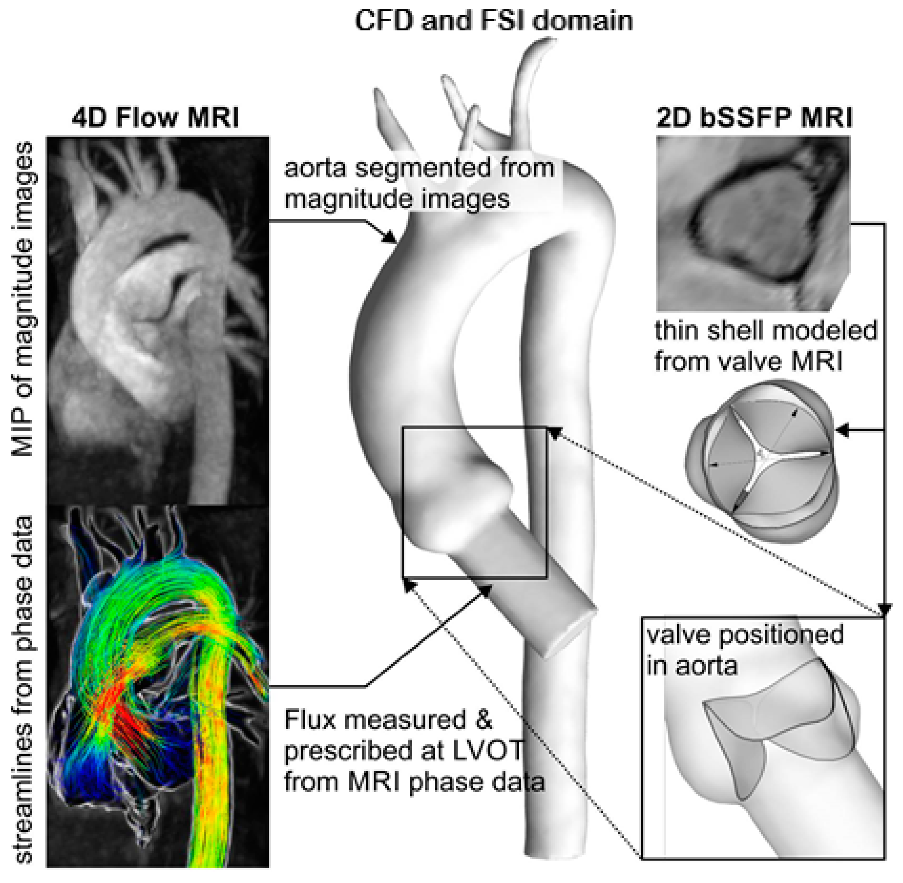
4D flow MRI and 2D balanced steady state free precession (bSSFP) cine MRI were performed at 1.5 T (Magnetom Avanto, Siemens Medical Systems, Siemens Healthcare GmbH, Erlangen, Germany) to obtain a patient-specific geometry and fluid inlet boundary conditions for the computational model. Breathheld 2D bSSFP cine images were acquired with retrospective electrocardiogram (ECG) gating in order to reconstruct the orientation of the aortic valve cusps. The 4D flow MRI data were acquired during free breathing using respiratory and prospective ECG gating, with settings as described previously [
24]. The resulting data provided complete volumetric coverage of the thoracic aorta geometry and allowed for segmentation of aorta and quantification of 3D blood flow velocities. Velocity encoding was set to 1.5 m/s, and the pulsatile flow waveform was measured with a cut plane placed orthogonal to the left ventricular outflow tract. The measured flow patterns and patient-specific aorta model were used to inform the computational framework, as shown in
Figure 1.
2.2. Equations for the Fluid Domain
The FSI problem considered here consists of a solid body representing the heart valve and aorta
submerged in an incompressible Newtonian fluid occupying a volume
bounded by
. The leaflets of a heart valve are represented as three-dimensional surfaces and modelled as thin flexible shells [
22]. While the shape of aorta was assumed to be realistic, its deformations were neglected. Therefore, it was simulated as a rigid, not a deformable, surface. The fluid and leaflet surfaces were in contact at the interface:
. Note that throughout this work, bold symbols are used for vectors, tensors, and matrices. The regular and italic symbols are reserved for scalar and vector/tensor components, respectively.
The fluid boundary consisted of three non-overlapping parts:
. Here,
are the stationary boundaries on which Dirichlet and/or Neumann, respectively, boundary conditions are specified, and
is the part along which coupling between the fluid domain and the solid phases of the problem needs to be specified. The interphase
is moving, so its configuration needs to be determined by solving the FSI problem. The equations governing the motion of Newtonian incompressible fluid in a domain
are the Navier–Stokes equations and the continuity equation, which in vector/tensor notation read:
In the above equations,
is the density of the fluid,
is the material or Lagrangian time derivative,
is the fluid velocity vector, and
is the Cauchy stress tensor for fluid. The above equations are subjected to various boundary conditions for the velocity
on the various segments comprising the fluid boundary. On the Dirichlet portion of the boundary
, Dirichlet boundary conditions are specified:
where
is a known function on the Dirichlet boundary. On the Neumann segment of the boundary, a stress boundary condition of the following form may be applied:
where
is a known function specifying the load on the Neumann part of the boundary or the unknown interaction forces with the solid and
is the unit vector normal to the
boundary and pointing away from
.
The specific values of the parameters describing blood are provided in
Section 2.4, dedicated to the details of the computational procedure.
2.3. The Equations for the Solid Domain
The momentum equations for the solid part were formulated in the current configuration and have the following form:
where
is the density of the material,
is the Cauchy stress tensor for a solid structure,
is the displacement of a material point, and
is the velocity of the material point. The boundary of the solid structure can be represented as the sum of non-overlapping parts
, where the indices
D and
N denote boundaries with Dirichlet and Neumann conditions, respectively:
Here,
represent the portions of the surface of the body in its current configuration where Dirichlet and Neumann conditions are applied, respectively,
is a traction vector acting on the surface,
is a unit vector normal to the boundary and pointing away from
, whereas
is the velocity prescribed on the surface. For FSI problems, additional boundary conditions must be implemented on
:
In the present situation where the solid domain is comprised of the valve leaflets modeled as a thin shell, is the surface representing the moving structure configuration, which needs to be determined by solving the FSI problem, vector is the (unknown) traction vector, which acts on this part of the fluid boundary, and are the stress tensor and the unit vector normal to the fluid boundary and specified earlier.
The fluid solver is based on the curvilinear immersed boundary (CURVIB) approach [
26]. For the structural solver, the finite element (FE) model proposed by [
22] was used. For more details, the reader is referred to [
19], where the capabilities of the proposed CURVIB-FE-FSI algorithm were demonstrated by applying it to simulate several problems of increasing complexity, all involving FSI with thin flexible structures. Details of the implementation of the nonlinear anisotropic constitutive model for real simulation of native aortic valves based on the rotation-free finite element approach were presented in [
20,
21].
Constitutive Relations for the Tissue Material
To investigate the effect of the heart valve leaflet thickness (anomalous in the natural heart or designed in the artificial valve) on the hemodynamics, we employed the modified May–Newman and Yin’s (MNY) material model. The version of the MNY model used in this work incorporates nonlinear and nonisotropic properties, which are characteristic of soft biological tissues [
27]. In fact, previous studies showed that MNY is among the most suited models to describe the response of biological tissue in heart valves, vessel walls, etc. [
28]. The parameters used in the calculations were taken from the literature and were previously used to analyze heart valves. Their specific values are provided in
Section 2.4, describing the simulation results.
As is often done in nonlinear elasticity, the constitutive MNY model discussed in this section will be associated with a specific form of the strain energy function
, where
,
, and
is the deformation gradient (see, e.g., [
29]). The corresponding second Piola–Kirchhoff stress is then
. The Cauchy stress presented in Equation (4) is related to
through the formula
T, . The associated tangent elastic properties, necessary in the iterative solution of the resulting nonlinear equations, are
.
The strain energy function for the adopted MNY model was introduced in [
27,
29,
30]. With subsequent modification proposed in [
31], it has the form:
To include incompressibility, use was made of the Lagrangian multiplier approach, which modifies the strain energy function as follows [
29]:
In the above equations,
(i.e., it is the trace of
C with
being a unit vector defining the local direction of material anisotropy,
,
for incompressible material. By invoking the usual variational arguments,
can be found [
29] to be
with
,
. As a result, the second Piola–Kirchhoff stress is:
where
is the second-order identity tensor,
. The principal directions for aortic valve fibers were defined as the circumferential (first) and radial (second) principal directions, respectively [
5].
In the finite element formulation of thin structural models, such as those used in modeling of the heart leaflets here, some special evaluation of the above equations is needed; this was discussed in [
20,
21].
2.4. Computational Details
In this work, we simulated a realistic, patient-specific aorta anatomy including the ascending aorta and the supra-aortic branches, which deliver blood to the brain. Including these branches is important for realistic FSI simulations, given that about 15–20% of blood is shunted to the brain through the brachiocephalic, common carotid, and left subclavian arteries. In what follows, and for the sake of brevity, we shall refer to aorta with the supra-aortic branches simply as “aorta”. We reconstructed the aorta anatomy from MRI data, as described below, immersed the resulting 3D anatomy into a background curvilinear grid that encloses, but is not fitted to the aorta walls, and treated both aorta and valve leaflets as immersed boundaries using the CURVIB approach.
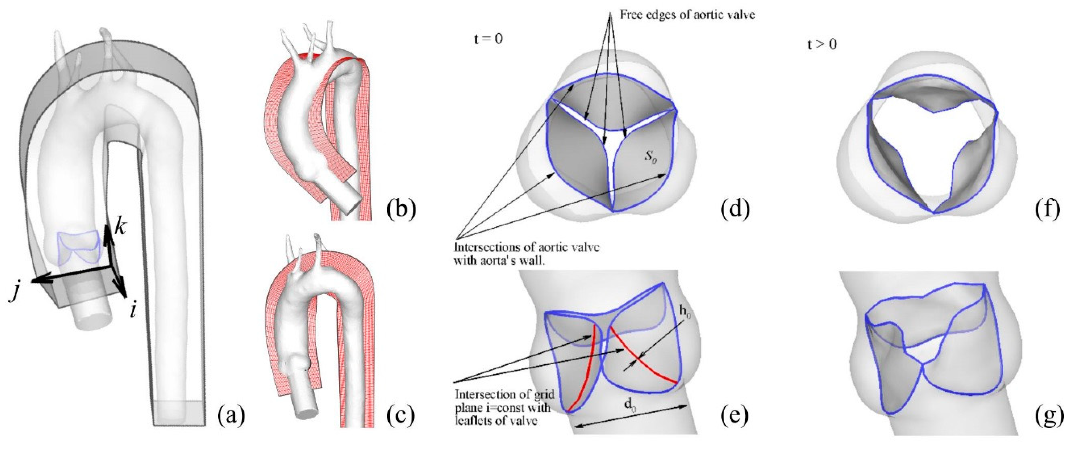
The overall computational domain is shown in
Figure 2, where a curvilinear fluid grid represents the curved computational domain that contains aorta with
nodes in the two transverse
and streamwise
directions, respectively. Surfaces of the rigid anatomic aorta and a tri-leaflet flexible heart valve were immersed in the fluid region. The leaflets of the heart valve were discretized with 476 triangular shell elements, while the surface of aorta was discretized by 23,892 triangular elements. The effective diameter of the valve was equal to
0.032 (m). The leaflets thicknesses to simulate calcification were considered to be constant and equal to three different values:
. Their mass density was equal to
.
The inflow boundary condition was prescribed at the inlet of aorta domain corresponding to the systolic phase of the cardiac cycle during which the aortic valve opens and closes. This inflow was used to specify time-dependent Dirichlet conditions for the velocity at the inlet. A cerebral blood flow at the branches of aorta was modeled as Dirichlet outflow boundary conditions for the velocity with 15% of the cardiac output. At the outlet of aorta, the zero-gradient Neumann condition was applied for all three velocity components
. No-slip and no-flux boundary conditions were applied on all solid surfaces (aorta and valve leaflets). The valve diameter
was used as the characteristic length scale, and the mean velocity
at the peak of systole was used as the velocity scale. Using the viscosity of blood
and blood density
gave a peak systolic Reynolds number Re = 3820 and Womersley number
, which were well within the physiologic range [
32,
33]. The non-dimensional time step for the simulations was set equal to
. Since the density ratio for this problem was of order one (
), the strong coupling FSI iteration with the Aitken non-linear relaxation technique [
34] was required for stable and robust simulations. In all subsequently-presented simulations, 4–10 strong coupling iterations were sufficient to reduce the residuals by 8 orders of magnitude. Our code was parallelized and used the Petsc Library (
https://www.mcs.anl.gov/petsc/). The simulations we report herein were carried out on a cluster with a dual 8-core AMD 6112. To estimate the efficiency of the code, we reported the CPU time per node of the computational grid, per processor and per number of time steps. For the heart valve problem, this quantity was equal to tCPU/(Nodes·Procs·ntime) ≈ 3 × 10
−2 μs, where tCPU is total computing time in seconds, Nodes is the number of computational mesh nodes,·Procs is the number of processors, and·ntime is the number of time steps.
The realistic aorta considered in this work was constructed/segmented from MRI data and was simulated to be a rigid surface, but the leaflets of the aortic heart valves were modeled as a thin deformable shell using the rotation-free FE formulation of [
22]. Note that the resolution of MRI we used was insufficient to make a segmentation of the aortic valve leaflets. This info from MRI (
Figure 1) was merely used to orient the leaflets in the model correctly. We simulated the trileaflet aortic valve with the common orientation of its leaflets toward the sinuses (RCC, right coronary cusp; LCC, left coronary cusp; and NCC, non-coronary cusp); see Gilmanov and Sotiropoulos (2015) [
35]. A nonlinear anisotropic May–Newman–Yin model [
30] was used to describe the constitute properties of the leaflet tissue. The material properties, coefficients
,
, and
, of the MNY model were selected as
,
, and
. The MNY model and its relevance to natural heart valve simulations were discussed in [
20,
21].
2.5. Physiologic Modeling of Calcification
In order to illustrate the anticipated impact of the simulations proposed in this work, the effect of valve calcification was analyzed as an example. This problem was chosen because relevant MRI geometric and hemodynamic data were available and could be used for comparison. The data were not complete, as the material properties of the tissue and of the deposited calcium were not available. Under those circumstances, the progression of the calcific aortic valve disease on the development of downstream aortic hemodynamics was investigated by changing valve leaflet thickness, which increased both its stiffness and its mass, as expected for this specific problem. The normal thickness of the simulated aortic valve ranged from 0.5–2.0
[
36]. Thus, to simulate calcification, the thickness of the valve cusps was increased sequentially within the range of
. The model results for these three cases were used to calculate hemodynamic parameters associated with clinical guidelines, as well as those used in the prosthetic valve research domain, to understand the level of hemodynamic disturbance induced by the progression of valve calcification. The shape of aorta in the model was reproduced from the MRI images.
2.6. Parameters Used to Characterize the Non-Steady Blood Flow
The aortic orifice area (AOA) depends on the structural, anatomical, and dynamic properties of the aortic heart valve and can impact both blood flow, as well as cardiac function. In practice, the AOA can be a direct or indirect measure of the size of the orifice when the valve is fully opened. Typically, the AOA is defined by one of the three methods [
37], i.e. (1) the geometric orifice area (GOA); (2) the effective orifice area (EOA); and (3) the Gorlin area (GA). The GOA represents the real orifice surface and can be estimated directly from MRI data, as well as from computational results; thus, we selected this parameter to estimate the AOA. In addition to GOA, the maximum velocity across the valve, which is often used clinically to estimate the degree of valve obstruction [
38,
39], was calculated form the simulation results. Finally, additional research parameters that characterize unsteady blood flow were selected to characterize the transvalvular hemodynamics comprehensively. In all, six different parameters were employed and are summarized below:
(1) The GOA, which is defined as:
where integration is carried over the surface of all three heart valve leaflets (in their current configuration),
is a surface of the aorta’s cross-section at the position of the heart valve (
Figure 2d),
is a unit vector normal to the flat surface
, and the symbol
is a vector representing the infinitesimal oriented area of the leaflet, while
is the projection of the opening through which the blood flows on the plane of leaflet attachment. Low GOA values (<1.5 cm
2) indicate clinically-relevant stenosis caused by a sclerotic valve.
(2) The maximum velocity
of the jet passing through the aortic orifice area, which is widely used in clinical practice to approximate pressure drop across the aortic valve using the simplified Bernoulli equation [
40] (
.
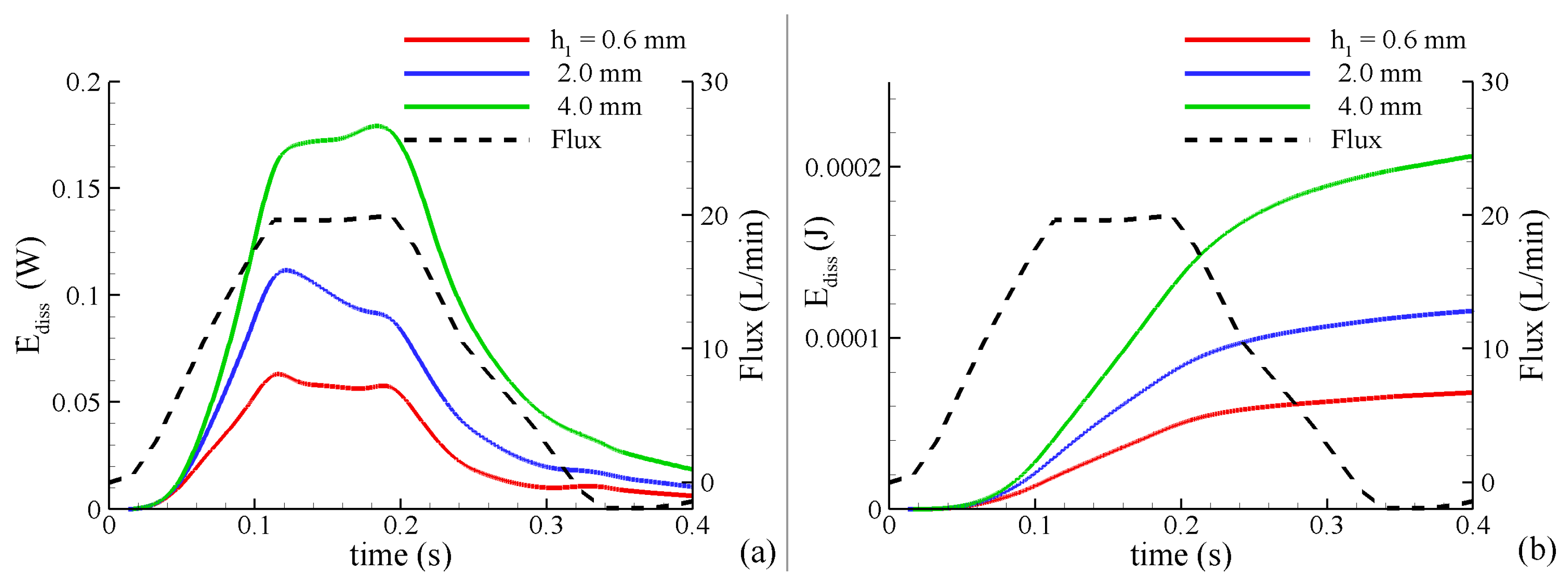
(3) The rate of energy dissipation, a measure of the instantaneous loss of power measured in Watts: where is a dissipation function, is the viscous shear stress tensor, and is the power loss in the entire thoracic aorta. This quantity characterizes the shear-related loss of energy caused by dissipation due to the viscosity of fluid flowing within aorta and to other obstructions such as stenosis of the cross-sections.
(4) The total loss of energy
, which characterizes the loss of energy during the cardiac cycle T.
represents the unrecoverable mechanical energy and is observed clinically as a permanent pressure drop across the valve. It is a more robust measure than pressure drop across the valve due to its insensitivity to pressure recovery [
23].
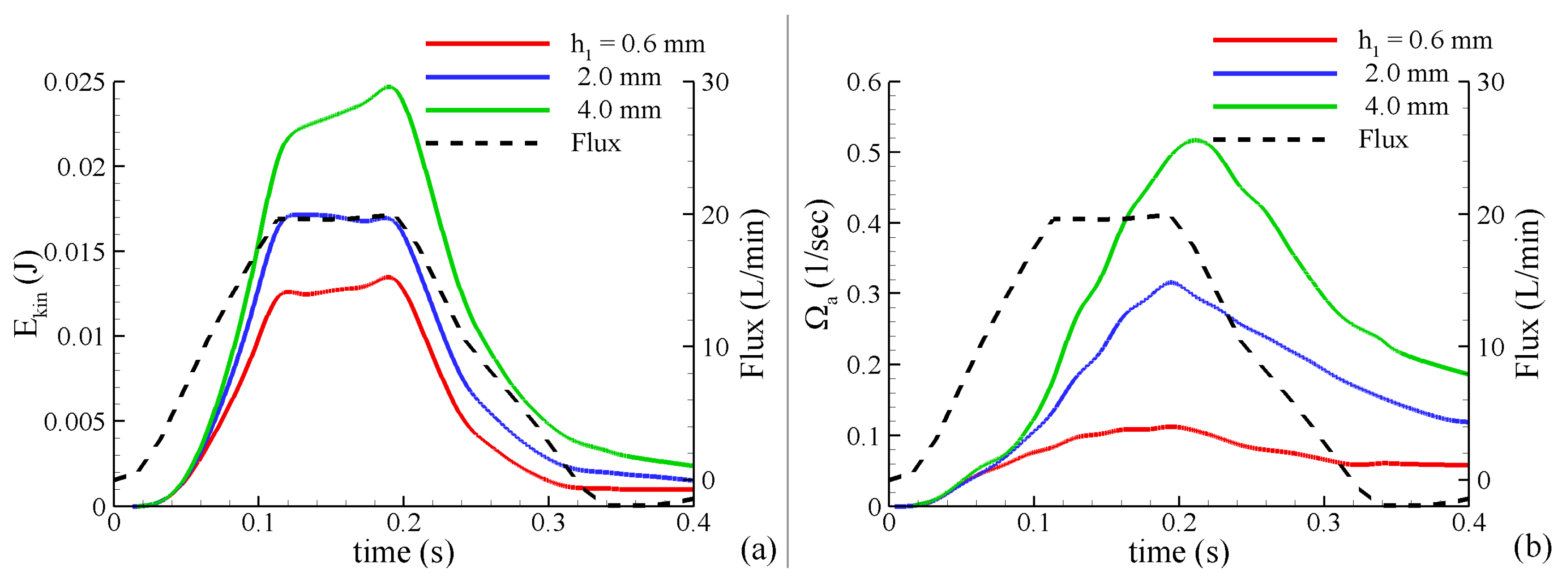
(5) The kinetic energy of the blood flow: where is determined by direct integration over the aorta’s volume. represents a portion of the mechanical energy in the system, which is exchanged with pressure and the viscous dissipation terms. In the absence of additional energy added to the system, an increase in kinetic energy will be accompanied by a decrease in pressure and an increase in energy dissipation.
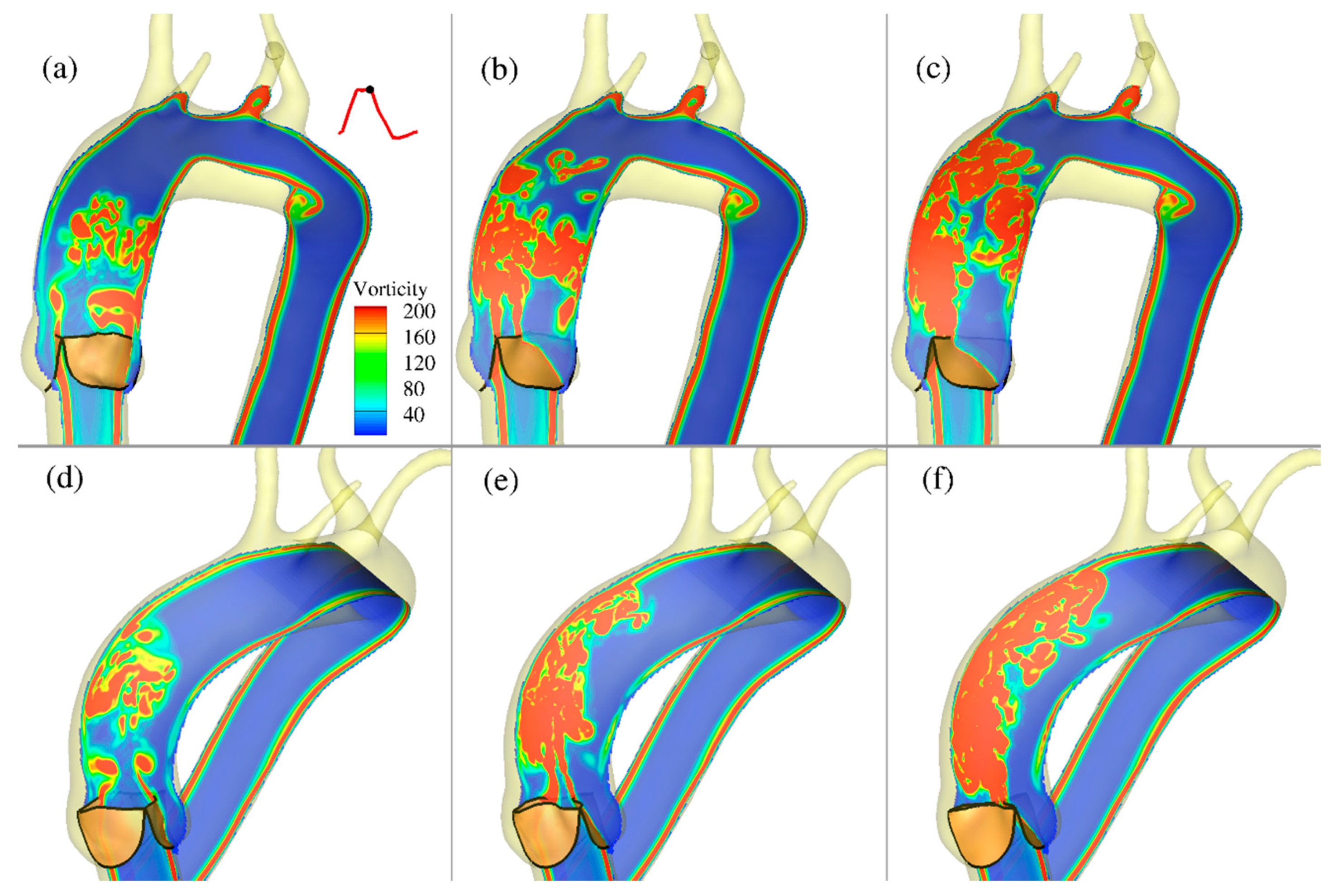
(6) The average magnitude of vorticity in the volume of aorta:
where
. Vorticity is a useful term illustrating the degree of fluid disturbance and has been widely used to evaluate the design of valve prosthetics [
41].
All these characteristics were calculated from the results of the FSI simulations during the systolic time period obtained from temporally-resolved MRI (.
4. Discussion
It is understood that any changes in the heart valve tissue properties, not only changes in their thickness, will lead to concomitant changes in hemodynamics. For example, in [
21], it was shown that the constitutive properties of the valves’ material might have a profound influence in this regard, and some diseases (or injuries) may be well modelled by variation in the valve’s material properties alone. Other pathological cases may require variation in the shape of the valve leaflets, or variation in both shape and properties. All these, and other, cases can be analyzed using FSI CFD models such as the one we employed herein.
It is also understood that in the case considered herein as an example, modeling calcification by increasing valve thickness involves significant simplifications. Among them is the assumption that mechanical properties of the calcified layer are the same as those of the original, uncalcified leaflets, that their mass densities are the same, and that the thickness of the leaflets is constant over their surface. Those features can in principle be included, when the data needed to build a better model become available. However, given that dynamic analysis is needed to analyze the problem addressed herein, modeling calcification just by changing the leaflets’ thickness captures important effects in the dynamics’ inertia (mass), which cannot be quantified by variation in the material properties alone. Inertia effects are particularly important when a highly nonlinear (and thus more realistic) model of the leaflets’ tissue is employed, as done in this work. For example, any changes to the inertial aspects of a dynamic problem will cause associated changes in the spatial and temporal distribution of the strain fields, which are further magnified by the nonlinearity of the material response. Thus, the approaches presented here are important intermediate steps toward the development of a comprehensive model capable of modeling realistic valve dynamics and aorta motion. In spite of the simplifications, our simulations yield new insights regarding the potential impact of calcification on the resulting complex 3D blood flow patterns.
In this study, the CURVIB-FE-FSI numerical approach [
19] was employed to carry out efficient simulation of the complex FSI problem of an aortic heart valve in an anatomically-realistic aorta with supra-aortic branches. To the best of our knowledge, the analysis presented herein and the results obtained constitute the first high-resolution quantitative FSI description of how physiologic blood flow in an anatomically-realistic aorta with supra-aortic branches is affected by changes caused by calcification of the valve leaflet tissue modeled by varying leaflet thickness. The various levels of calcification were shown to be associated with profound differences regarding the resulting flow patterns and in the magnitude of the vorticities, and hence the forces imparted on the walls of aorta and on the valve leaflets. In particular, by comparing the effects caused by increasing the valve leaflet thickness (to simulate calcification), a corresponding reduction of the aortic valve orifice area and increase in transvalvular velocity resulted from the simulated calcification. The effect of the calcification gave rise to significantly different hemodynamics, both near the valve and downstream in the ascending aorta. These effects are known to have negative consequences for the function of both the left ventricle and proximal ascending aorta [
45].
A fluid–structure interaction solution with more realistic model of aortic valve calcification was reported in [
13]. However, in [
13], aorta was simplified to be in the shape of circular cylinder, and no supra-aortic branches were considered. Nevertheless, the reported numerical results for the peak flow velocity and the aortic orifice area were shown to be consistent with those seen in clinical observations, [
38,
39]. Remarkably, our results with a simple model of the valve calcification, but a more realistic model of aorta, were also consistent with the clinical observations reported in [
13]. In our simulations the peak flow velocity is ranging 1.4–3.3 (m/s) and the aortic orifice area is ranging 4.3–1.3 (
, depending on the valve thickness
. In the clinical observations [
13], the peak flow velocity is ranging from
and the aortic orifice is ranging from
to
for healthy and moderate stenosis, respectively. The agreement of those two sets of results with clinical observations can be considered to be partial validation for both the results presented in [
13] and those presented in this work. A better (or full) validation would need to relate to measurements corresponding to one specific patient and the numerical results that are based on a model correctly representing all essential features of that patient anatomy and disease, which include both the real aorta and advanced calcification model (if calcification is the problem).
Limitations
It is recognized that in the diseased aortic valve, the situation is complex since calcification occurs non-uniformly, resulting in irregular leaflet surface and increasing the complexity of the flow patterns. This should be considered in assessing actual clinical flow data from stenotic valves. There are other hemodynamically important aspects such as deformations of realistic aorta with aortic root and supra-aortic branches, occurring in response to varying pressure, for example, that should be considered for a realistic description of the problem. To our best knowledge, no existing work is that comprehensive.
The main goal of the present work was to develop a model versatile enough to facilitate analysis of various problems, of which calcification is but one example. Other possible applications may include the changes related to aging, for instance. That was the reason why “calcification” was not mentioned in the title of the paper. To facilitate various possible applications, a shell heart valve model based on numerical through-thickness and over-the-surface integration was used. In the future, that will allow for easy introduction of the variable thickness of the diseased valve and for inclusion of dissimilar materials across its thickness, such as a layer of biological tissue combined with irregular deposits of calcium. We believe that incorporation of all those possible generalizations in this “first” effort would be warranted only in the analysis of a very specific case of the diseased heart. Then, computational results could be validated against the measurements conducted on that specific heart. Without such measurements, inclusion of valve irregularities and different properties of deposited calcium could not be validated. Their influence could only be illustrated, and the significance of that would not be very different from the illustration of the effects of varying valve thickness presented in this work. In view of the above reality, our paper focused on the hemodynamic changes often observed in the presence of aortic stenosis. It has been demonstrated that the proposed model is capable to capture the increase in peak velocity and the decrease in GOA independently of whether stenosis is associated with calcification or any other disease. Clearly, the specific type of disease will require some additional modification of the model and will have different quantitative effects. Thus, our future work will focus on validation in actual patient cases in which imaging, echo, and other data are available. It is noted that the simulations presented here did not consider the contact between the leaflets in the valve’s closing phase. Consequently, no information is provided regarding the flow during diastole. This aspect of the formulation is currently under development. The main difficulty is that in the systolic phase (open valve), one deals with one, connected computational fluid domain, while in the diastolic phase, when the valve is closed, this domain breaks into two disconnected domains. Experimental data characterizing the actual heart valve in each case of interest are also a work in progress. In the case of calcification of the natural valve, the spatial (and temporal) variation of the calcification thickness and its mechanical properties (along with the properties of the heart tissue, of course) have to be simulated. Depending on the availability of data characterizing the problem, possible approaches range from treating leaflets as three-dimensional structures with variable geometry and material properties, to treating the valve as layered thin shells with spatially-varying thickness.
5. Conclusions
Although the results presented here related to valve calcification, the approach used is capable of handling many other scenarios for which the requisite data are available. Even the specific (and approximate) model of a calcified valve, used here as an example, demonstrates that reliable and useful information regarding hemodynamic changes downstream from the affected valve could be extracted using FSI algorithms described in this work. Some results, such as the decrease of the GOA with the increasing thickness of the valve, may seem intuitively natural, but that observation is only of value when it is quantified, which does require complex FSI analysis. The same is true of other results obtained here, such as the values and distribution of WSS, velocity distribution, and energy of the flow. They all affect the functioning of the heart and are likely to guide decisions made by medical professionals.
Several possible future extensions of the approach used in this work are possible. In the case of the calcified valve problem, more realistic valve calcification models, as well as inherent aorta motion would be one example of such extensions. In other heart anomalies, it could be the geometry of the leaflets, variations between the leaflets in terms of their mechanical properties, variations in the shape of aorta, etc. Incorporation of those features in the model is possible if the data sufficient to describe them are available. For that reason, such further development must be driven by the needs of the medical community; this work was meant to show that all that is now possible.


