Stenosis Indicators Applied to Patient-Specific Renal Arteries without and with Stenosis

Abstract

Pulsatile flow in the abdominal aorta and the renal arteries of three patients was studied numerically. Two of the patients had renal artery stenosis. The aim of the study was to assess the use of four types of indicators for determining the risk of new stenosis after revascularization of the affected arteries. The four indicators considered include the time averaged wall shear stress (TAWSS), the oscillatory shear index (OSI), the relative reference time (RRT) and a power law model based in platelet activation modeling but applied to the endothelium, named endothelium activation indicator (EAI). The results show that the indicators can detect the existing stenosis but are less successful in the revascularized cases. The TAWSS and, more clearly, the EAI approach seem to be better in predicting the risk for stenosis relapse at the original location and close to the post-stenotic dilatation. The shortcomings of the respective indicators are discussed along with potential improvements to endothelial activation modeling and its use as an indicator for risks of restenosis.

1. Introduction

When severe enough, a renal artery stenosis (RAS) leads to hypertension and impaired renal function. RAS may have different etiologies, e.g., fibromuscular dysplasia or being of atherosclerotic character (denoted as ARAS). In 90% of cases, RAS is caused by arteriosclerosis [1]. Although much less common than other manifestations of atherosclerotic disease, the condition can be present in the range of 3–7% in a healthy population [2]. Similar to atherosclerotic disease in general, the prevalence increases with age. For certain patient groups with severe heart disease, a prevalence of 54% has been observed. Conversely, patients with newly discovered RAS often have cardiovascular disease with widespread arteriosclerosis [3]. The overall mortality is increased up to 6 times in patients with atherosclerotic RAS compared to healthy subjects of similar age [2].

Arteriosclerotic changes are predominantly found in certain arteries (coronary, carotid, renal and femoral) at certain locations (bifurcations, branches and at strong curvatures). The impact of hemodynamics in atherogenesis (i.e., plaque formation) has been recognized for many decades [4]. Moreover, it has been hypothesized that the process is related to the Wall Shear Stress (WSS) [5], claiming that both high WSS [6] as well as low and, in particular, oscillatory WSS [7] can play a role in the processes. The latter mechanism appears to be more frequently associated with intimal thickening. In recent years, the temporal- and spatial-gradients of the WSS has been recognized as equally important factors as the magnitude of the WSS itself [6].

There is no consensus in the precise definition of RAS [2]. However, according to the American Heart Association (AHA), RAS is defined as hemodynamically significant if one or more of the following criteria are fulfilled [1]:

• a narrowing of the vessels’ inner diameter between 50% to 70% by visual estimation with a peak translesional pressure gradient of at least 20 mmHg (2.67 kPa) or a mean gradient of at least 10 mmHg (measured with a 5 F (about 1.6 mm) or smaller catheter or pressure wire at conventional angiography),
• a stenosis of at least 70% narrowing (inner diameter) measured on a conventional angiogram, and
• a stenosis greater than 70% narrowing (inner diameter) by intravascular ultrasound measurement.

RAS shows subtle or no symptoms before the disease becomes severe [2] and is usually presented with hypertension that is often resistant to drug therapy. Treatment options include antihypertensive medication and reduction of risk factors [2]. In some cases, angioplasty with dilatation and stenting of the affected artery is an alternative. Although the patency of the renal artery is improved after revascularization therapy, the clinical outcome for the patient is not necessarily beneficial [8,9]. Hence, medical therapy is considered as a first option. The main issue with revascularization is the long-term effect as discussed by Lao et al. [1] and the references therein. After having a progressive ARAS over a longer period of time, the damage to the kidneys can be irreversible [10]. Moreover, as revascularization does not eliminate the underlying reasons for the disease, it is not surprising that a continuation of the atherosclerotic process is observed also postoperatively.

Numerical simulation of the flow in renal arteries and its relation to renal artery stenosis (RAS) was recently reported [11,12]. In the present study, four indicators are considered in order to assess the possibility of relapse of atherosclerosis/stenosis after revascularization. Three of these markers, namely time averaged wall shear stress (TAWSS), relative residence time (RRT) and oscillatory shear index (OSI) have been used in literature for stenosis identification in blood flow simulations in arteries, most commonly in the carotid artery [13]. The relevance of these indicators has been questioned in the review of Peiffer et al. [14]. The fourth marker has not previously been applied as an indicator for stenosis.

2. Materials and Methods

2.1. Patient Cases

For this study, three patients who had underwent Computed Tomography Angiography (CTA) were selected.

• Two patients with a left sided ARAS (at common locations for the stenosis)
• A previously healthy patient undergoing an acute CTA study of the aorta, where no pathological changes were found (except minor atherosclerotic changes that could be considered as a “normal” finding considering the patient’s age).

The patients having ARAS underwent conventional angiography and treatment with dilatation and/or stenting of the stenosis.

The CTA data was used to define the geometry of the abdominal aorta, also including the celiac trunk, the superior mesenteric and renal arteries. Siemens Somatom Flash Scanners, having a limit of 0.3 mm isotropic voxels, were used to carry out the CTA study with slice thicknesses of 1 mm and 0.75 mm. The reason for the difference is advances in imaging software improving the quality and noise reduction for the image rendering carried out in 2015 and 2017. For the image reconstruction, Siemens SAFIRE I30 (iterative reconstruction algorithm) was applied. Iodine contrast used for the CT angiography showed a concentration in the abdominal aorta of about 300–500 HU.

The shape of a sclerotic artery has randomly distributed irregularities, making it difficult to distinguish these from noise in the CTA data. Here, the software Mialab by Wang and Smedby [15] is applied to perform the segmentations (i.e., the process of generating the three-dimensional shape of the aorta), utilizing threshold-based techniques. The effect of the segmentation approach on the arteriosclerotic indicators has recently been investigated by Berg et al. [16]. The inside wall of the abdominal aorta was delineated from the level of the diaphragm down to right above its bifurcation, including the celiac trunk, the superior mesenteric artery and the renal arteries.

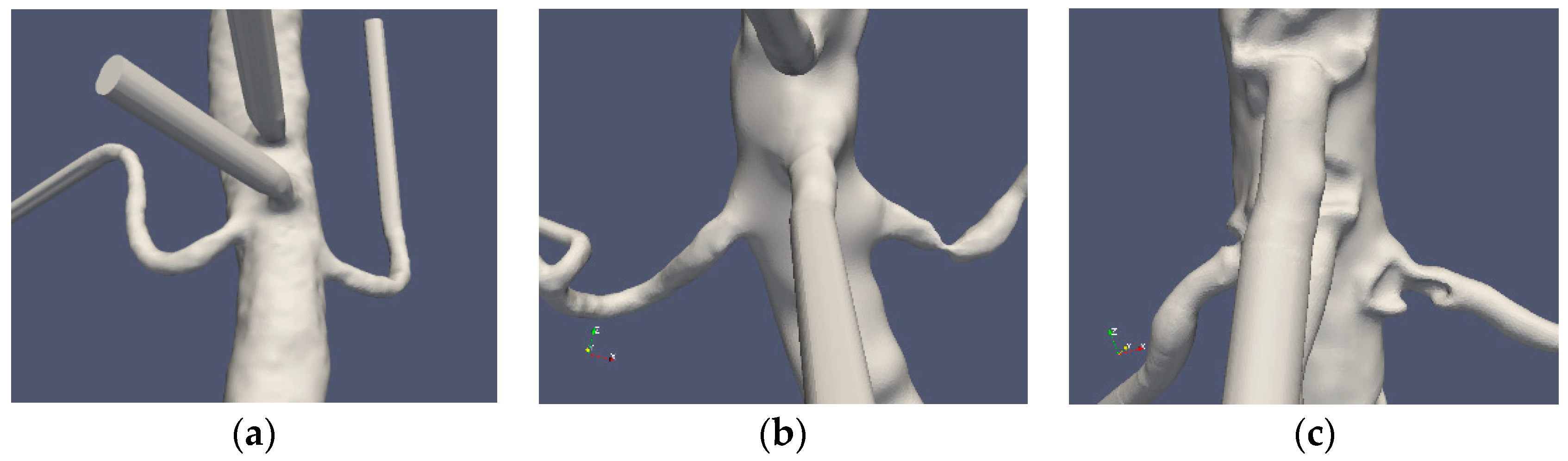
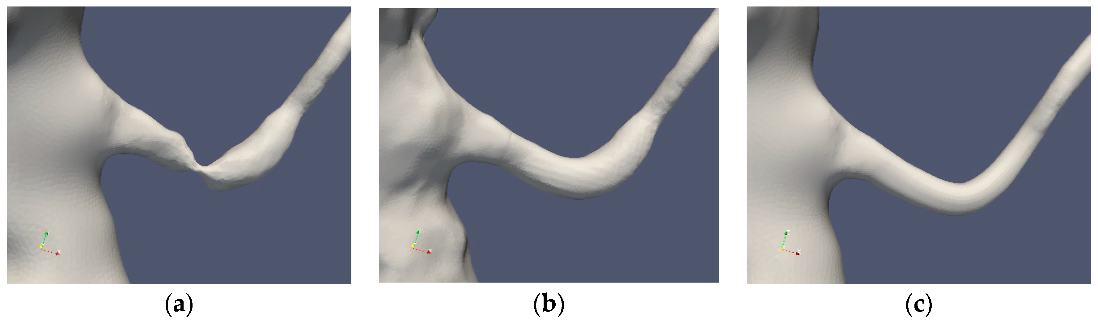
In patients 1 and 2 (termed as Case1 and Case2 in the following), the affected renal artery was reconstructed. In Case1 reconstruction was made using two different computational methods. For Case2, computational reconstruction was unfeasible due the stenosis location close to the vessel ostium. Therefore, reconstructions were created manually by removing the stenosis and, in a second step, by post-stenotic dilatation, using the graphics software Blender [17]. Further smoothing of the surface geometry was applied to mimic the smoother shape commonly obtained in a revasculated and stented artery. Moreover, no attempt was made to reshape the artery into a circular cross section. The reconstructed arteries were used to assess the applicability of the abovementioned indicators.

The computational domain (including the abdominal artery and the main arteries bifurcating from it, namely the celiac trunk, superior and inferior mesenteric arteries and the renal arteries) was used for the blood flow simulations presented here.

2.2. Governing Equations

The blood was considered to be an incompressible non-Newtonian fluid and modeled as a mixture of Red Blood Cells (RBC) and plasma (solution of proteins, electrolytes and other small molecules in water). The volume fraction of RBCs (hematocrit) is denoted by α. The density of RBCs and plasma were ρ_α = 1100 kg/m³ and ρ_p = 1025 kg/m³, respectively. The mixture density ρ = ρ_α·α + ρ_p (1 − α) varied in space and time. However, the density of the RBCs and plasma being similar allowed for the mixture to be approximated as being incompressible. Thus, the Navier–Stokes equations for the conservation of mass and momentum can be expressed as

$$\frac{\partial u_i}{\partial t}+\frac{\partial (u_i{u}_j)}{\partial x_j}=-\frac{1}{\rho }\frac{\partial p}{\partial x_i}+\frac{\partial }{\partial x_j}\nu \frac{\partial u_i}{\partial x_j}$$

(1)

$$\frac{\partial u_i}{\partial x_i}=0$$

(2)

where u_i is the mixture velocity in the ith direction, p is the pressure and ν is the kinematic viscosity of the mixture. The RBC phase, and thereby the blood, is assumed to behave as a continuum. This assumption is based on the large difference in scales concerning the diameters of the arteries and the RBC (6 ×∙10⁻³ m and 6 ×∙10⁻⁶ m, respectively). Thus, the RBCs were assumed to be transported by the mixture (advection) and diffusion:

$$\frac{\partial \alpha }{\partial t}+u_i\frac{\partial \alpha }{\partial x_i}=\frac{\partial }{\partial x_i}D\frac{\partial \alpha }{\partial x_i}$$

(3)

where D represents the diffusivity of the RBC phase. In the following, the RBC diffusivity is assumed to be constant with D = 10⁻⁸ m²/s, corresponding to the largest diffusivity value as presented by Casa and Ku [18].

The conservation of mass and momentum (Equations (1) and (2)) are so-called incompletely parabolic. In the steady state, the system is elliptic and requires three conditions on all boundaries. Similar boundary conditions are assumed to be needed in the time-dependent case. A wide range of boundary conditions may be applied, provided that the normal to the inflow and outflow surfaces are such that the total mass conservation is satisfied.

2.3. Rheological Model

There exist several models for blood viscosity dependence on α and the shear rate, γ [19]. In the following, the Quemada model is used [20]. The Quemada model has been adjusted for a wide range of hematocrit as well as shear rates and has been described as well-suited for modeling blood rheology in a range relevant to clinical situations [21]. The apparent viscosity of the blood is modeled by the following expression:

$$\mu ={\mu }_p{\left(1-\alpha \frac{k(\gamma ,\alpha )}{2}\right)}^{-2}$$

(4)

where the plasma viscosity μ_p = 1.32 × 10⁻³ Pa s, γ is the magnitude of the shear-rate tensor ${\gamma }_{ij}=\frac{1}{2}\left(\frac{\partial u_i}{\partial x_j}+\frac{\partial u_j}{\partial x_i}\right)$ and

$$k(\gamma ,\alpha )=\frac{k_0(\alpha )+k_{\infty }(\alpha )\sqrt{\gamma /{\gamma }_c(\alpha )}}{1+\sqrt{\gamma /{\gamma }_c(\alpha )}}$$

(5)

The coefficients k₀(α), k_∞ (α) and γ_c(α) are given by

$$k_0=e^{3.874-1041\alpha +13.8{\alpha }^2-6.738{\alpha }^3}$$

(6)

$$k_{\infty }=e^{1.3435-2.803\alpha +2.711{\alpha }^2-0.6479{\alpha }^3}$$

(7)

$${\gamma }_c(\alpha )=e^{-6.1508+27.923\alpha -25.6{\alpha }^2+3.679{\alpha }^3}$$

(8)

The model accounts for the shear thinning property of the blood; hence μ decreases with an increasing γ, consistent with experimental observations. When the diffusivity of α is small (as used in the cases herein) and the inlet condition of the RBC concentration is uniform, α remains constant throughout the computational domain and over time.

2.4. Centerline and Geometrical Parameters

The centerline of the artery is useful to characterize vessel geometry as well as for post-processing. Simply, the centerline can be defined as the path inside the vessel, between two points (at the vessels inlet and outlet), maximizing the total distance to the boundary [22]. In this study, the centerlines were computed using the Vascular Modeling Tool Kit, VMTK [23], computing all lines from the aortic inlet to the outlets. To evaluate the effects of the vessel geometry, the surface curvature was calculated using VTMK. From the two principal curvatures k₁ and k₂, also known as maximum and minimum, the Gaussian curvature, K = k₁·k₂ and the mean curvature M = (k₁ + k₂)/2 was obtained.

2.5. Wall Shear Stress and Wall Indicators

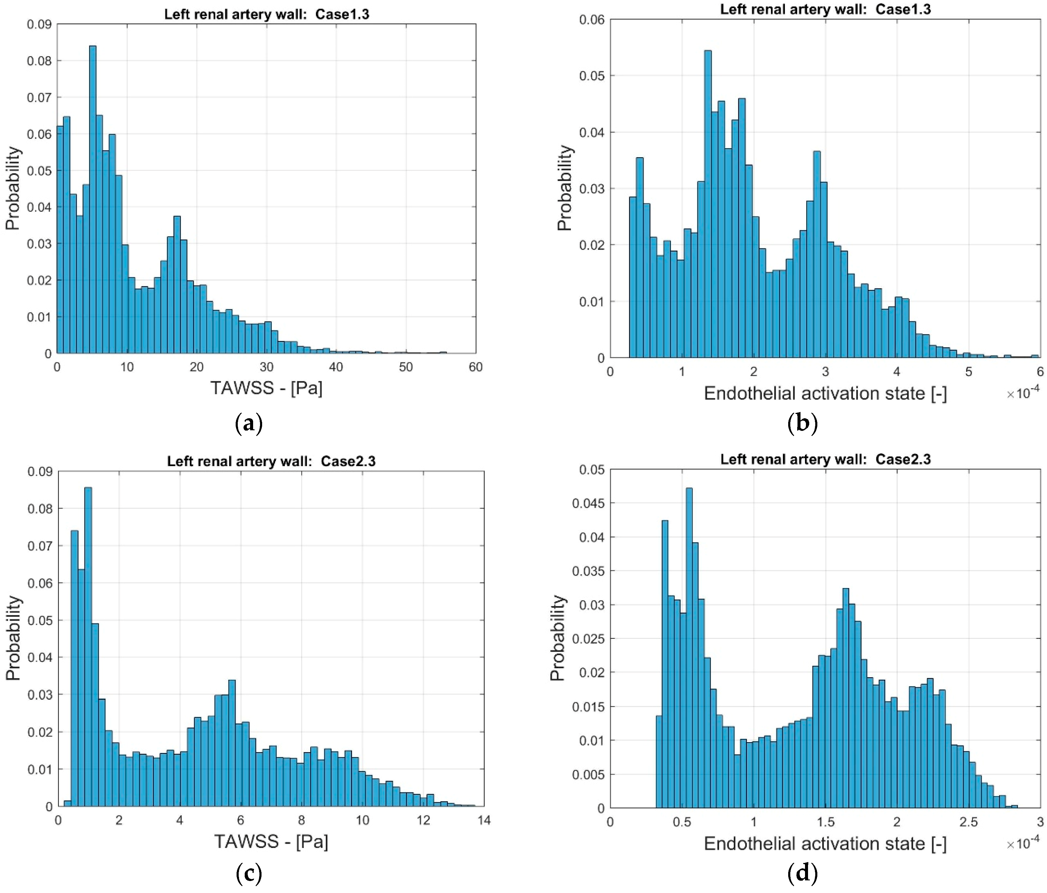
From the shear stress tensor τ_ij = μ·γ_ij on the wall of the vessel and the unit normal to the wall (n_j), the wall shear vector WSS_i = τ_ij·n_j can be defined. This vector defines the force per unit area acting on the endothelium. The component of the wall shear stress vector, normal the wall, is denoted by WSS_Ni = (WSS_j n_j) n_i. If n_i is normal to the wall, the planar components (WSS_pi) are given by WSS_pi = ε_ijk WSS_j n_k or WSS_i − WSS_Ni n_i. As the WSS is commonly accepted as a crucial parameter for the formation of atherosclerosis, several WSS-based indicators for the presence of stenosis has been presented. To directly measure WSS in vivo and even in mock-loops using water is difficult. Hence, time-averaged values of the components of the WSS that are parallel to the surface under consideration (i.e., WSS_i) is most commonly found in literature. The following four indicators were used to assess the flow data.

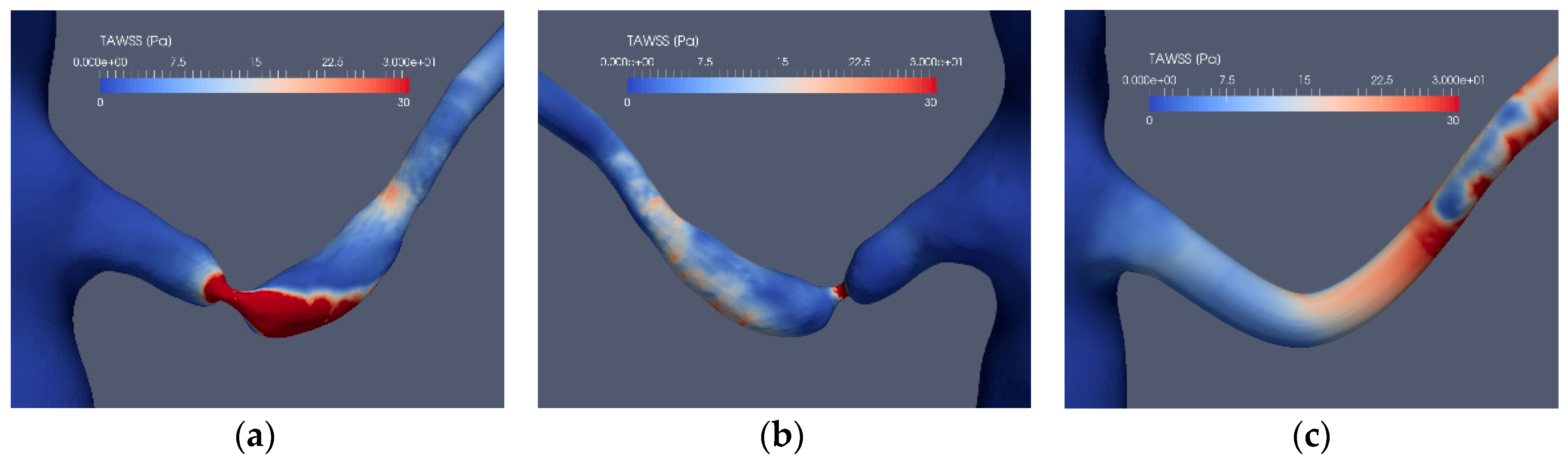
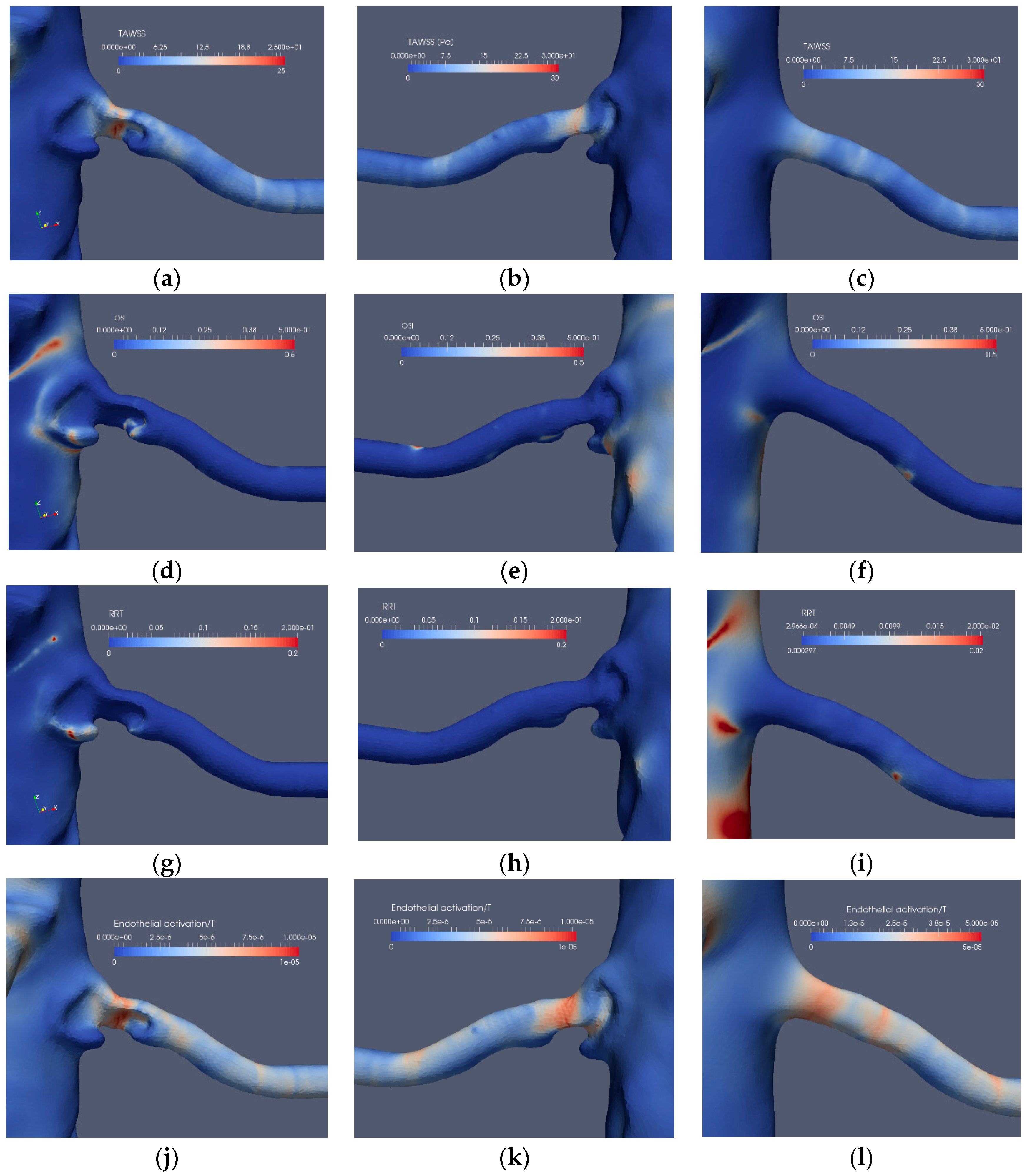
2.5.1. Time Averaged Wall Shear Stress (TAWSS) [24,25]

$$TAWSS=\frac{1}{T}{\displaystyle \underset{0}{\overset{T}{\int }}\left|WS{S}_i\right|dt}$$

(9)

TAWSS is the time-averaged value of WSS vector magnitude. TAWSS is a local value and does not contain information regarding the temporal or spatial WSS variations. TAWSS cannot be lower than 0 but has no definitive upper bound. Computed values of TAWSS may be compared to the measured data for the few and simple cases for which such data exists. It has empirically been observed that oscillatory WSS promotes atherosclerosis. However, this information is not included in TAWSS. To at least partially account for such an effect, the following indicator was introduced:

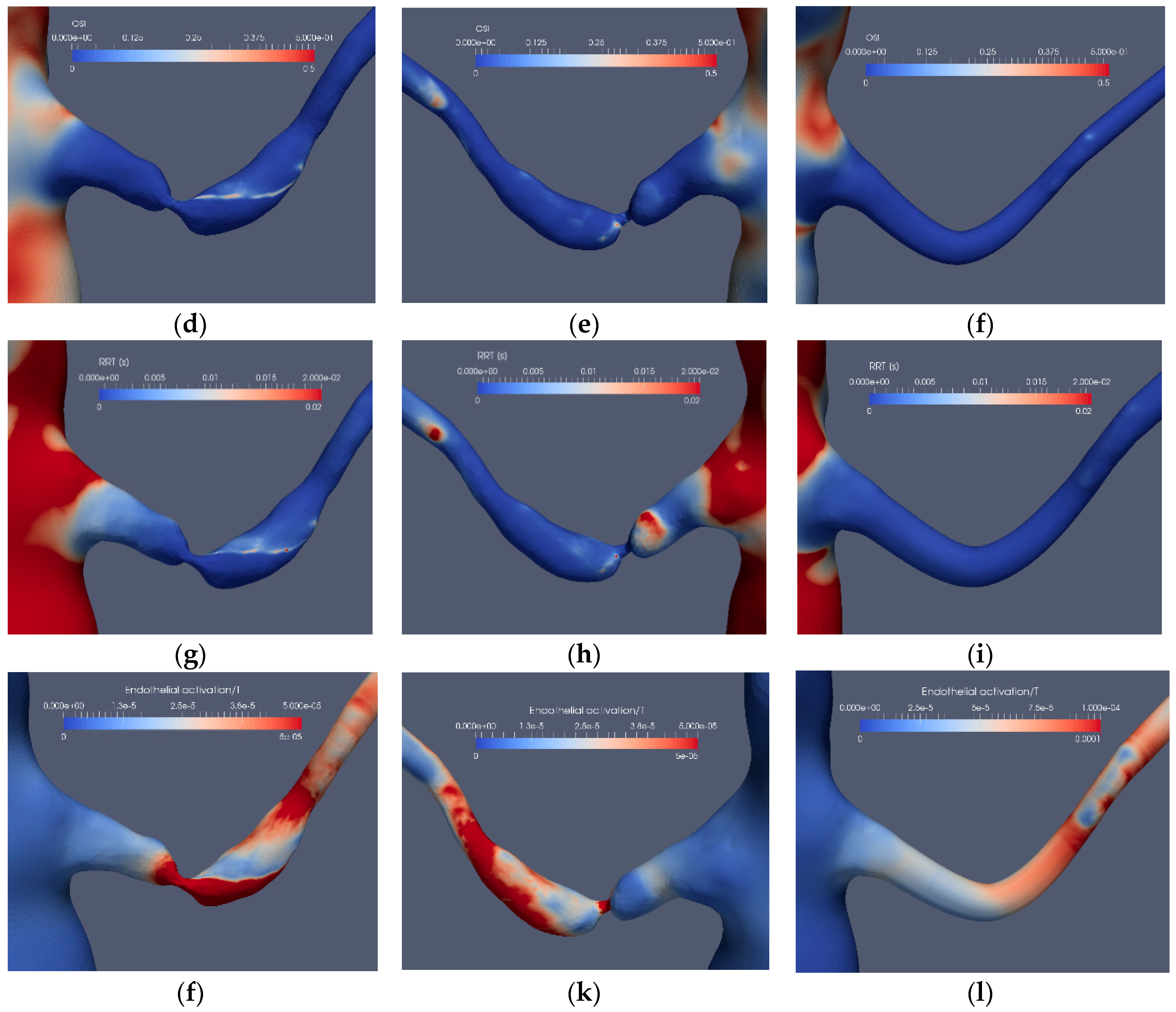
2.5.2. Oscillatory Shear Index (OSI) [25,26]

$$OSI=\frac{1}{2}\left(1-\frac{\left|{\displaystyle \underset{0}{\overset{T}{\int }}WS{S}_{i}dt}\right|}{{\displaystyle \underset{0}{\overset{T}{\int }}\left|WS{S}_i\right|dt}}\right)$$

(10)

OSI varies between 0 and 0.5. When WSS_i is strictly positive (oscillatory or non-oscillatory), OSI = 0. When WSS_i changes signs such that the integral of the positive and negative sequences are the same, OSI obtains the value 0.5. Values of 0 < OSI < 0.5 indicate an oscillatory WSS field, but the indicator does not indicate the amplitude nor frequency of the oscillations. The time during which extreme WSS (high or low) exists appears to be essential for the development of atherosclerosis. Low TAWSS (< 4 dynes/cm²) and significant OSI (>0.15) are risk factors for the incidence and progression of atherosclerosis [27,28].

2.5.3. Relative Residence Time (RRT) [29]

$$RRT=\frac{1}{(1-2\cdot OSI)\cdot \frac{1}{T}{\displaystyle \underset{0}{\overset{T}{\int }}\frac{\left|WS{S}_i\right|}{\mu }dt}}$$

(11)

RRT includes both OSI and TAWSS. From Equation (11), it can be noted that RRT is related to the time-mean of the shear-rate and not the residence time of a fluid or a real particle. For OSI = 0, the time scale is proportional to the viscosity and inversely proportional to TAWSS.

2.5.4. A Fourth Indicator of Atherosclerosis is Proposed Herein

As endothelial activation is associated with the activation of other cells, similar activation models could possibly be applied also for endothelial cells. Here, the power law model of Nobili et al. [30] for platelet activation is applied. Analogous models have been used for RBC destruction due to elevated shear. In the platelet activation model, the target variable, the Platelet Activation State (PAS), was defined as the fraction of platelets that have become activated relative to all platelets in the tested blood. The model has three empirically determined parameters: a, b and c [31]. In our study, the target variable is denoted endothelial activation index (EAI), using the same numerical values for the model parameters as suggested by the original model for platelets.

$$\frac{dPAS}{dt}=c{\tau }^{b/a}{H}^{a-1}and\frac{dH}{dt}={\tau }^{b/a}$$

(12)

τ is the so-called scalar stress, corresponding to the length of the WSS vector. The following values of the parameters were used: a = 1.3198, b = 0.6256 and c = 10⁻⁵ [30]. The dose term, H, contains the accumulated stress whereas the instantaneous effect of stress enters through the scalar stress. It can be noted that the stress effect is computed as the scalar stress to the power of b/a = 0.474. This numerical value has no real physical meaning; it is rather the result of fitting the model parameters to the experimental data (PAS). Moreover, it is noted that EAI, as PAS, is a dimensionless number, interpreted as the probability of activation of an endothelial cell. The meaning of H and τ^b/a is less clear as these entities contain dimensional variables to some power.

The PAS-based indicator differs in essence from the former three as it indicates the time evolution of the activation level. TAWSS, OSI and RRT are, on the other hand, time-averaged quantities that do not attempt to indicate the temporal effect of the WSS.

2.6. Numerical Methods

The meshes for all cases were generated using STAR-CCM+ (v12.04.11, Siemens, Alameda, CA, USA). The flow simulations were carried out using the open software package OpenFOAM (v5.0, CFD Direct Ltd, Reading, UK) [32]. A formally second-order finite volume discretization was used to approximate Equations (1)–(3). The diffusive fluxes were computed using central differences while the convective fluxes were computed with limited central differences. The time derivatives were approximated to second order with an implicit backward time stepping scheme. The time step was adapted to allow for stability (Courant number restriction) and speed. Thus, the time step was in the range of 10⁻⁴ s and 2 ∙ 10⁻⁶ s where the smallest time steps were applied during peak systole for the stenoted artery cases where the mesh size and the high flow speed dictates the smallest time steps. The discretized equations were solved sequentially, starting with the RBC transport (Equation (3)) coupled to the flow equations through the density and viscosity fields. The momentum equation was solved component by component, after which three pressure correction steps with the PISO algorithm were carried out to ensure that velocity field satisfies continuity (Equation (2)).

3. Computed Cases

In the following, the three patient cases that were considered are described. As described in the Materials and Methods section, CTA data was used to generate a computational domain of the original geometries. In the stenoted cases, the affected arteries were reconstructed whereby the stenosis was removed by different approaches. Further smoothing was used to a large extent to eliminate the post-stenotic dilatation that normally can be observed downstream of the stenosis.

3.1. Geometrical Data

Three patient cases were considered: one normal and two stenoted. Case0 is denoted as “normal” although the aorta and the renal arteries do exhibit typical non-smoothness associated with atherosclerosis. Case1 and Case2 represent the two patients having renal artery stenosis. The segmentation of the original CTA data is denoted as Case1.1 and Case2.1, respectively. The segmentations of both cases were further redefined in order to emulate the shape of the renal arteries after surgery. These segmentations were made manually with certain level of smoothing, denoted as Case1.2, Case1.3, Case2.2 and Case2.3 for the two patients, respectively. The original shapes of the abdominal aorta and the renal arteries for the three patients are depicted in Figure 1.

Table 1. The curvature and spatial resolution of the segmented arteries.

Case	Curvature	Stand Dev	Grid Size	Grid Size	Grid Size
	(1/m)	(1/m)	(106 cells)	(min) (m)	(mean) (m)
Case0 Normal Aorta	2111	249	4.3	7.5 ×∙10−5	2.8 ×∙10−4
Case1.1 Stenoted Artery	6407	295	3.3	3.1 ×∙10−5	3.5 ×∙10−4
Case1.2 Voronoi	3411	647	1.3	1.2 ×∙10−5	4.7 ×∙10−4
Case1.3 Mesh Sweep	1357	128	2.7	6.0 ×∙10−5	3.7 ×∙10−4
Case2.1 Stenoted Artery	5515	592	5.9	2.9 ×∙10−5	2.4 ×∙10−4
Case2.2 No Stenosis	2224	226	8.9	2.7 ×∙10−5	2.1 ×∙10−4
Case2.3 Smooth	1137	152	3.5	6.5 ×∙10−5	2.9 ×∙10−4

summarizes the cases under consideration. The segmentations of Cases 1 and 2 are depicted in Figure 2 and Figure 3, respectively. The standard segmentation (Case1.1) was derived directly from the CTA picture (Figure 1b). The left renal artery was reconstructed by removing the stenosis using a Voronoi scheme (Case1.2) [16]. A smoother segmentation, removing also the post-stenotic dilatation, denoted as “mesh sweep”, is marked as Case1.3. The proximal stenosis case was segmented (Case2.1, original) and two smoothed cases (Case2.2 and Case2.3). The three segmentations of the two patients are depicted in Figure 2 and Figure 3, respectively.

3.2. Characterization of Geometries

In order to quantify the smoothness of the segmentations, the regularity of the arterial surface or the deviation of the shape of the artery from a cylinder with a possibly variable diameter along its axis can be considered. For the former measure, the radii of curvature of the surface may be used. For a smooth vessel, the larger value of the curvature will correspond to the radius of the vessel, whereas the minimal value of the curvature corresponds to the surface gradient in the axial direction. For a straight cylinder, the latter value will vanish. The curvature for the different cases was computed, and the minimal curvature values are given in Table 1.

3.3. Boundary Conditions

Several minor branches such as the inferior mesenteric, lumbar, phrenic and ovarian/testicular arteries of the aorta are not present in our simulations. The geometries were restricted to the abdominal part of the descending aorta. In order to reduce the effects of inlet boundary conditions, the inlet section was prolonged by 4 inlet aortic diameters. The inlet conditions that were applied specified the velocity vector and the RBC concentration distribution. The inlet to the abdominal aorta was assumed to be pulsatile with a time-dependent flow-rate. The in-plane component was assumed to vanish, and the normal component obtained from an aortic flow simulation [33] and its temporal variation is given in Reference [16]. At the inlet plane, the inlet velocity profile was taken to be flat. The RBC concentration was assigned a top hat profile (α = 0.45), having a lower concentration in the near wall region such that α = 0.25 tanh(R_e − r)/ε) + 0.2. At the wall boundary of the artery, the RBC concentration was 0.2 and increasing towards the central parts of the artery depending on the parameter ε. For the computational cases herein, ε = 0.025.

All branches of the aorta were elongated in order to reduce the effect of the outlet boundary conditions. Such an elongation was, in particular, important for the renal arteries. Benim et al. [34] provides typical flow rates at the main branches of a human artery. In this work, flow rates close to those of Benim were applied, with the main deviation in terms of the boundary conditions on the renal arteries. Benim applied a flow rate of 10% of the inlet on each boundary. Instead, we applied a constant pressure at the outlet planes of the renal arteries. The flow rates used for the celiac trunk, superior mesenteric artery and the aortic outlet were 22%, 22% and 33%, respectively. Hence, the total flow rate through the renal arteries was about 23%. However, the division between the two arteries depended on the resistance of the respective arteries. The condition on the RBC transport was set to zero gradient along the axis of the artery.

3.4. Limitations

Several assumptions were made during this work. We assumed that blood is a mixture having a uniform density but locally varying viscosity depending on the local shear-rate and hematocrit. The variations in hematocrit were small due to the assumption made on the diffusivity of the hematocrit transport Equation (3). Thus, natural hemodilution effects are at large neglected. This current study assumes that the arteries are rigid. However, this may be a reasonable assumption in patients with RAS who often have general atherosclerotic disease in their large arteries. Moreover, a major uncertainty in all numerical simulations stems from boundary conditions. The inlet conditions depend not only on the axial flow (more often available) but also on the secondary, in-plane flow that in turn depends on the upstream shape of the aorta (and in particular the arch of the aorta). Furthermore, outflow conditions are non-trivial due to the effects of compliance. At the outlet of the renal arteries, two sets of pressure conditions were applied: one constant and the other corresponding to a measured time-dependent pressure [34]. However, the two different conditions do not alter the results with respect to the indicators.

4. Results

In the following, a qualitative description and quantitative characterization of the geometries and the corresponding segmentations are provided. Typical flow features due to the different geometries and segmentations are presented. Thereafter, the impact of the flow field on the WSS and corresponding indicators is assessed. The ability of these indicators to form a predictive tool for identifying future stenosis is considered and discussed.

4.1. Computational Accuracy

Table 1 shows the spatial resolution used for the different geometries. A grid refinement study was carried out to assess the adequacy of the spatial resolution [16]. Figure 4 depicts the pressure and losses across the stenosis during the heart cycle (Case1.1), using 2 and 4 million computational cells, respectively. Considering the pressure drop over the affected left renal artery, the root mean square difference between the two grids during one heart cycle normalized with the fine grid pressure drop was 2%. The corresponding value for the pressure losses was 3%. A similar comparison of TAWSS and OSI (not showed here) revealed a maximal relative difference less than 5%.

4.2. Segmentation Characteristics

According to the above, the curvature was used to characterize the smoothness of the segmentation. Table 1 summarizes the values of these parameters for the seven cases considered here. As mentioned in the Methods section, the CTA data had a slice thickness of 1 mm for Case1 and 0.75 mm for Case2 and Case0. This level of resolution may induce noise that will be reflected in the curvature. This effect is observed in the non-smoothed cases. The first smoothing (Case1.2 and Case2.2) maintained the irregularity of the post-stenotic dilatation, whereas after the secondary smoothing, the curvature became smaller. Optimally, the radius and the bend of the artery can be recovered from the minimal and maximal values of the curvature. In our computational cases, the arteries are not smooth enough to determine these characteristic values. Moreover, the surface roughness is reflected by the standard deviation computed over the artery surface.

4.3. Flow Characteristics

The shape of the aortic-arterial branching along with the geometrical shape of the artery and the stenosis determine the resistance and the flow rate in the artery. A considerable difference is observed between the axial and the in-plane velocity components among the different patients and segmentations. The branching angles of the three left renal arteries are close to each other. The axial velocity profile is close to uniform with a peak of about 1 m/s. Also, the flow has a swirling component, observed in the cross-sectional velocity components (not shown).

Figure 5 depicts the axial flow component for 5 cross sections of the segmented original and reconstructed artery: Case1.1, Case1.2 and Case1.3. The flow in the stenoted artery (Figure 5a) has the character of a swirling jet, where the jet increases in intensity closer to the arterial wall, implying an enhanced shear stress at this location. Closer to the center of the artery, a weak reversed flow is observed, formed due to the entrainment of the strong swirling jet. The strong variation of the axial flow in space and time leads also to elevated shear stress (SS) and in particular at the wall (WSS). Compared to the stenoted artery, the flow in the Voronoi reconstructed artery (Figure 5b) is more uniform, with some remaining geometrical irregularities observed in the proximity of the location of the stenosis. The acceleration of the flow is found at the end of the post-stenotic section leading to uniform axial flow. The reconstructed segmentation using mesh sweeps (Figure 5c) removed both the stenosis and the post-stenotic dilatation, resulting in a nearly uniform axial flow with a peak flow of about 2 m/s. This value is similar to that of the Voronoi segmentation that, in turn, is lower as compared to the peak velocity in the stenoted case, corresponding to approximately 3 m/s.

Figure 6 shows the in-plane flow at the same cross sections as in Figure 5, where the cross sections are colored by the axial velocity components and the arrows display the in-plane velocity. The in-plane velocity is roughly one order of magnitude smaller as compared to the axial velocity component. The effect of the stenosis and the reconstruction can be noted. The most upstream plane includes a section of the aorta showing the vortex upstream of the stenosis, a vortex also observed downstream of the stenosis that is stronger than the axial velocity component (Figure 6a). Removing the stenosis by the Voronoi approach affects the upstream flow as compared to the stenosis case. After the bend, the proximal part exhibits a Dean-like double vortex that becomes a single vortex further downstream (Figure 6b). An increase of the axial flow is noted at the end of the post-stenotic dilatation where the cross section area decreases (Figure 6b). The mesh sweep segmentation (Figure 6c) shows a gradual increase in the axial components as the area of the artery reduces from about 0.25 cm² to about 0.1 cm². The in-plane flow is induced by the curvature of the artery in contrast to the other two segmentations where the abrupt area reduction contributes to the strength and shape of the in-plane velocity.

The flow in the artery with a stenosis close to the bifurcation from the aorta is largely affected by the blocking effect of the stenosis. The axial flow in the three segmentations (Case2.1, Case2.2 and Case2.3) is depicted in Figure 7. The bifurcation angle is less sharp than in the artery shown in Figure 5. In this artery, the stenosis blocks the flow from the aorta, forming a jet and backflow in the regions “shadowed” by the stenosis. The separated flow region extends to less than one diameter downstream the stenosis. The axial velocity component is nonuniform and is turning mildly along the artery due to the nonsymmetric shape of the stenosis. The cross-flow in the artery is depicted in Figure 8a, where the in-plane circulation in both the separated flow region and along the artery is depicted. The in-plane flow for the stenoted artery (Figure 8a) includes a vortex such that the flow direction in the two downstream planes is in opposite directions. The flow in the artery has roughly the same character during the heart cycle, but the strength of the in-plane flow is weaker as compared to the change in the axial flow. The non-stenoted segmentation (Figure 7b and Figure 8b) depicts the axial velocity and the in-plane velocity at peak flow, respectively. The axial flow has a minor defect (nonuniformity) in the proximal region at the central part. The flow develops axially further downstream as the cross-sectional area decreases. Due to the bends of the renal artery, the axial symmetry of the axial velocity component is broken. The in-plane motion shows the swirling motion (Figure 8b). In the proximal plane, the central part has no in-plane flow, whereas the off-center flow is strong (about 1/3 of the axial component in the same plane). Further downstream, a relatively strong in-plane flow is shown, although the directions are switched.

The reconstructed smoothed artery (Figure 7c and Figure 8c) exhibits an almost uniform axial flow except at the concave wall in the two downstream planes. The profile appears to have an inflection point at higher flow rates. However, this does not lead to flow instability, mainly due to the short duration of this potentially unstable mechanism. The in-plane flow exhibits a large single vortex in the first two cross sections. In the third plane, the vortex is incomplete, although a weaker vortex is noticed in the fourth plane. The temporal development of the in-plane flow during the aortic cycle shows the development of a central vortex that decreases in strength at a rate of the axial velocity component.

4.4. Stenosis Indicators

The indicators described in the literature to identify the presence of flow irregularities and in particular for stenosis (TAWSS, OSI and RRT) were applied to the reconstructed and normal renal arteries as well as to the aortic surface region near the affected renal artery bifurcation. In addition, the Nobili’s model [30] was applied as an indicator for endothelial activation (EAI).

Considering the application of the indicators for the stenoted renal artery, Figure 9 and Figure 10 depict the TAWSS, OSI, RRT and EAI for Case1.1, Case1.3, Case2.1 and Case2.3, respectively. As shown, TAWSS is strongest at the stenoted region for both cases. In Case1.1, TAWSS extends on one side of the vessel due to the inclination angle between the artery and the aorta and the asymmetry of the stenosis, generating a jet that hits the wall of the artery downstream of the stenosis. Moreover, this jet causes the post-stenotic dilatation. Except at the edge of the unsteady jet formed by the stenosis, the OSI signature (Figure 9d) is small at the stenosis, indicating that the WSS is weakly oscillatory except at the edge of the jet. The stenosis is not indicated by RRT. However, RRT displays a larger value upstream of the stenosis (Figure 9h). Due to an essentially non-oscillatory WSS, that in turn leads to low OSI values, RRT behaves as the inverse of TAWSS. Thus, among the common indicators (i.e., TAWSS, OSI and RRT), only TAWSS was able to locate the stenosis well in the stenoted artery of Case1.1. When applied to the reconstructed and smoothed artery (Case1.3), none of the indicators could predict a risk for stenosis at the site of the stenosis. However, TAWSS indicated an elevated value downstream of the artery bend characterized by larger axial and in-plane velocities, leading to elevated WSS. OSI and RRT do not indicate an elevated risk along the reconstructed artery.

Introducing the EAI indicator (Figure 9j–l), an increased value of EAI for the stenotic artery (Case1.1) is displayed, similarly as for TAWSS although with peaks not colocated. A similar behavior of EAI and TAWSS is also observed for the reconstructed artery, giving a weak indication at the location of the stenosis.

The corresponding results for the near bifurcation stenosis (Case2.1) are depicted in Figure 10. The stenosis is located close to the branching from the aorta and blocks a significant portion of the artery. TAWSS clearly indicates the stenosis location and shows a weak indication at another location (Figure 10a,b), probably also affected by minor surface unevenness. OSI has low values with the exception of minor regions upstream as well as downstream of the stenosis (Figure 10d). The low OSI value at the stenosis is due to the small spatial velocity fluctuations at that location. On the other hand, downstream of the stenosis, the shear-layer is unstable with spatial fluctuations. The frequency of these fluctuations can be estimated by approximating the relevant shear layer thickness (about 1 mm), and velocity scales (about 0.6 m/s) of the shear-layer combined with the Strouhal number of 0.3 known to be associated with shear-layers implies fluctuations at a frequency of a few hundred Hz. The RRT has low values (Figure 10g,h) due to its definition, i.e. it is proportional to the viscosity of the blood. The EAI clearly indicates the stenosis (Figure 10j,k), displaying only weak values in other regions, similar to TAWSS. The performance of TAWSS, OSI and RRT in the reconstructed and smoothed artery is similar to Case1.3, namely, only a weak indication of stenosis by TAWSS (Figure 10c), whereas OSI (Figure 10f) and RRT (Figure 10i) displayed small values. Moreover, EAI appears to also indicate the location of the stenosis (Figure 10l).

In order to further compare the indicators, the distribution of the frequency of the values of TAWSS and EAI were considered. Figure 11 depicts the probability distribution for the range of TAWSS and EAI for the two stenoted arteries. As noted, the range of TAWSS reaches values of almost 60 Pa (Case1.3) and 14 Pa (Case2.3). The higher TAWSS value is due to the smoothing process. The EAI is in the range of 3∙× 10⁻⁵ and 6∙× 10⁻⁴ (Case1.3). Furthermore, the range of EAI differs by one order of magnitude. For Case2.3, the distribution of the EAI shows two peaks that, to some extent, is also observed in TAWSS. The numerical values of TAWSS are relatively modest, below 14 Pa. However, the largest values are considered to correspond to the high shear that may lead to thrombosis [35].

5. Discussion

This work implicitly assumes that renal arteries developing stenosis and that are “revascularized" shall develop a new stenosis over time. This “assumption” has clinically been confirmed and is expected as the surgical treatment does not remedy the underlying atherosclerotic disease [10]. Therefore, the stenosis indicators are assessed in terms of their detection ability of the location of the stenosis in the reconstructed artery. Such an indicator could be used to determine the possible benefit of arterial revascularization. However, reaching this goal requires more cases to be considered, yet the results are useful in order to develop appropriate indicators that shall be predictive in the sense stated above.

The close connection between the endothelial activation and the activation of inflammatory cells as well as coagulation system is now well-established [36]. It is also reasonable that the response of different cells to external stress is similar to each other (through evolution). Thus, it is natural that similar models can be applied for the activation of endothelial cells, platelets and leukocytes.

The four indicators investigated do locate the stenosis in the affected artery. However, the level of success in predicting the potential risk for restenosis is less clear. The different indictors heavily rely on the WSS, well-motivated by the literature in the field. A major problem associated with the commonly used indicators is that WSS is a tensor and the variable called WSS by the indicators is a scalar. Different expressions of a tensor could be used that leads to a scalar expressing some property of the tensor. The different in vitro measurements of the effect of WSS on endothelial cells were assessed in a unidirectional flow [35]. The expression for WSS in such simple cases is a scalar. The flow in the renal artery is much more complex. 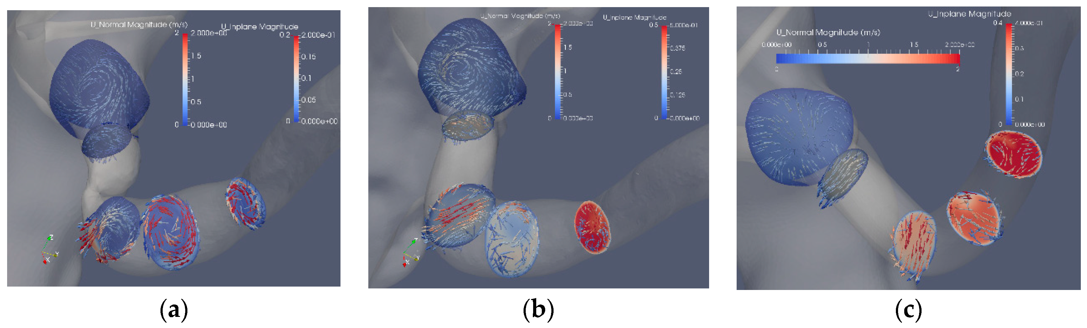As shown in Figure 6, Figure 7 and Figure 8, the flow is not always aligned with the centerline of the artery. 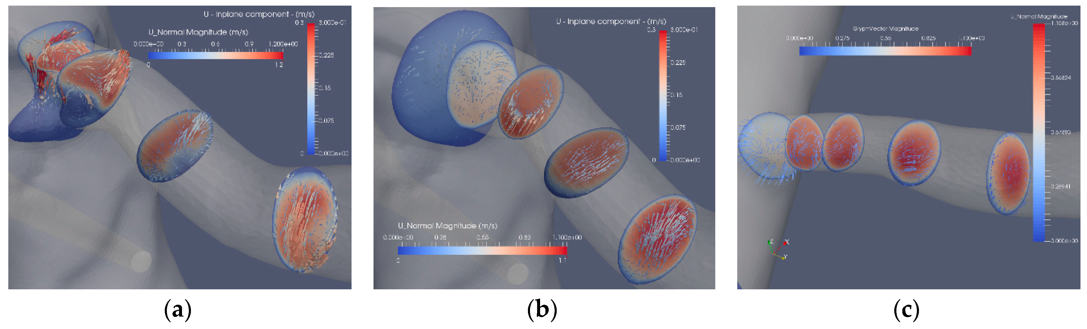Swirling flow leads to a WSS that has a component along the axis of the artery as well as another component along the circumference of the artery. This issue has been discussed in relation to platelet activation where all the components of the stress tensor may be important.

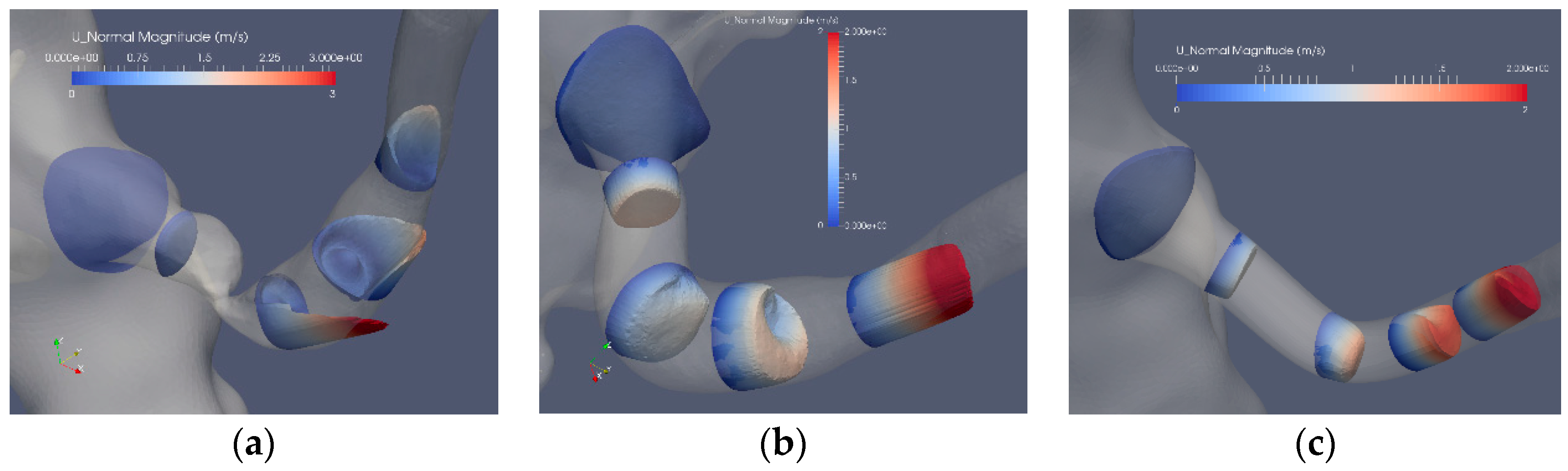
TAWSS was introduced as an indicator since the role of WSS for atherosclerosis was recognized for decades. TAWSS has a meaning when compared to a reference value. To this end, it has to be noted that it has experimentally been found that atherosclerosis may occur in low WSS as well as at high WSS regions. Therefore, to interpret TAWSS, threshold values for the “non-pathological” range have to be set. Hence, TAWSS can be used quantitatively only if empirical data can be relied upon, which appears to be case-dependent. TAWSS does not contain any impact of WSS transients on the endothelium. This poses an additional drawback as transients are known to play a role in low WSS cases. Despite these shortcomings, TAWSS did produce an elevated level in the reconstructed artery at the location of the stenosis in the non-reconstructed artery.

In contrast to TAWSS, OSI is sensitive to oscillatory WSS. However, this is the case only when the flow changes sign. OSI has a value of 0 for all oscillatory flows in which the flow is unidirectional, independent to the magnitude or the frequency of the oscillations. Thus, OSI may solely detect the edge of an oscillating separation bubble, independent of the frequency of the oscillation. This effect can be observed in Figure 9d and Figure 10d. The separation bubbles formed due to the post-stenotic dilatation were also located by OSI (Figure 9e and Figure 10e). Due to its construction, OSI has limited value in cases with significant oscillatory WSS, and it should not be used for assessing future risks for stenosis in revascularized arteries.

The relative residence time, RRT, has its basis in the observation that low flow and low shear regions are prone to the formation of thrombosis and become atherosclerotic (parts of Virchow’s triad). By this concept, prolonged residence time is a good indicator for a low flow region. The definition of RRT (Equation (11)) contains explicitly the viscosity as a parameter. This may lead to possible misinterpretation as RRT is not representing a diffusion process but rather the effect of vorticity. It would probably be more appropriate to replace the TAWSS term by the time average of the near wall vorticity as this would reflect a mechanism for prolonged residence time. In the cases investigated here, it was noted that RRT is largest at separated (high vorticity) regions. The indicator fails for the revascularized arteries as the near wall flow is smoother. For a more detailed prediction of the atherosclerotic process, the concentrations and residence times of cells and molecules would be needed. One possible option to achieve this is to use a Lagrangian Particle Tracking (LPT) approach, directly computing the residence time, instead of using RRT. Additionally, when using LPT, the details of mixing, cell/particle size and weight effects could also be accounted for.

Power law-based models such as Nobili et al. [30] are phenomenological in character and not designed to reflect the details of the process modeled. The model parameters are adjusted so that the target variable, in our case, the Endothelial Activation Index (EAI), is well-represented. The model does include the history effects of WSS on the endothelium, which is reasonable. In this sense, EAI differs from the other three indicators as EAI takes WSS history into account. However, the WSS history is considered in an unweighted manner. That is, the impact of a large WSS value is the same, independent of when it occurred. Thereby, cellular response and possibilities of cell repair known to occur are neglected. For the two cases considered here, the EAI model is performing well, both for the stenoted and the smoothed revascularized arteries. However, due to the inherent limitations of the power law approach, we suggest introducing another approach in partial analogy proposed more recently for platelet activation (Soares et al. (2013) and Consolo et al. (2017)). The idea is to add the contribution of various parameters such that the indicator remains bounded and by using dimensionless variables, so that each term has a functional and physical meaning. Such an indicator could, in addition to the local effect of WSS and the time-limited (or time-weighted) history effect of WSS, also include the effects of temporal- and spatial-variations of WSS. In this way, the low and oscillatory WSS contribution to endothelial activation and atherosclerosis enter explicitly into the expression for the indicator. Platelet activation models lack a repair and/or cellular response mechanism. Such a mechanism could possibly be more important in modeling the endothelial response. Since atherosclerosis is a slow process, it is reasonable to assume that the endothelial cells respond to WSS, strengthening their ability to withstand the elevated stress. The same applies to the response of the subendothelial matrix to the variability in the WSS.

In addition to the modeling of the atherosclerotic process on a macroscopic level, there are several other issues related to the models used in the present simulations. As already noted, the RBC transport should account for diffusion due to the lift effect on the cells in the presence of a velocity gradient. The RBC concentration becomes nonuniform that may affect the local viscosity and the WSS by a factor of up to two under the same flow conditions.

Another issue that has to be addressed is the setting of appropriate boundary conditions. As in practically all clinical situations, there is no available data on the flow conditions. To a large extent, such data is less useful since the flow conditions in the aorta vary considerably, depending on the activities of the patient. Thus, the flow in the aorta cannot be set to a single value or percentage of the cardiac output. One could remedy the need for a large number of simulations by including the boundary conditions in the governing equations and use that as a parameter. It is not only the flow but also its redistribution from the aorta that varies. Such a redistribution changes the phase angle between the pressure and flow and also in the renal arteries. Therefore, defining the four outflow conditions, needed by the numerical procedure, is a real problem. The effect of errors in boundary conditions on the global flow behavior may not be pronounced in global terms [37]. However, the effects of the flow details do enter in a pronounced manner in the WSS and thereby in the stenosis indicators. Thus, developing clinically appropriate boundary conditions is essential.

6. Conclusions

This paper assessed the possibility of using four different indicators for assessing the risk for developing a stenosis in revascularized renal arteries. Among the three common indicators, only the TAWSS indicated a possible risk for relapse, whereas the OSI and RRT did not. The proposed phenomenological cell activation model, previously used for platelet activation and applied herein to the endothelium (EAI), did indicate a potential risk for relapse. A promising extension, the phenomenological model would include the effects of temporal and spatial WSS gradients. The indicators must be evaluated on a larger group of patient-based CTA data to assess their clinical value.

References

1. Lao, D.; Parasher, P.S.; Cho, K.C.; Yeghiazarians, Y. Atherosclerotic renal artery stenosis—Diagnosis and treatment. Mayo Clin. Proc. 2011, 86, 649–657. [Google Scholar] [CrossRef] [PubMed]
2. Vassallo, D.; Kalra, P.A. Atherosclerotic renovascular disease—Epidemiology, treatment and current challenges. Postepy Kardiol. Interwencyjnej 2017, 13, 191–201. [Google Scholar] [CrossRef]
3. Plouin, P.-F.; Bax, L. Diagnosis and treatment of renal artery stenosis. Nat. Rev. Nephrol. 2010, 6, 151–159. [Google Scholar] [CrossRef] [PubMed]
4. Ku, D.N.; Zarins, C.K.; Giddens, D.P.; Glagov, S. Pulsatile flow and atherosclerosis in the human carotid bifurcation: Positive correlation between plaque localization and low and oscillating shear stress. Arteriosclerosis 1985, 5, 292–302. [Google Scholar] [CrossRef]
5. Texon, M. A hemodynamic concept of atherosclerosis with particular reference to coronary occlusion. AMA Arch. Internal Med. 1957, 99, 418–427. [Google Scholar] [CrossRef]
6. Dolan, M.J.; Kolega, J.; Meng, H. High Wall Shear Stress and Spatial Gradients in Vascular Pathology: A Review. Ann. Biomed. Eng. 2013, 41, 1411–1427. [Google Scholar] [CrossRef] [PubMed]
7. Huo, Y.; Wischgoll, T.; Kassab, G.S. Flow patterns in three-dimensional porcine epicardial coronary arterial tree. Am. J. Physiol. Heart Circ. Physiol. 2007, 293, H2959–H2970. [Google Scholar] [CrossRef]
8. Cooper, C.J.; Murphy, T.P.; Cutlip, D.E.; Jamerson, K.; Henrich, W.; Reid, D.M.; Cohen, D.J.; Matsumoto, A.H.; Steffes, M.; Jaff, M.R.; et al. Stenting and medical therapy for atherosclerotic renal artery stenosis. N. Engl. J. Med. 2014, 370, 13–22. [Google Scholar] [CrossRef]
9. Wheatley, K.; Ives, N.; Gray, R.; Kalra, P.A.; Moss, J.G.; Baigent, C.; Chalmers, N.; Eadington, D.; Hamilton, G.; Lipkin, G.; et al. Revascularization versus medical therapy for renal-artery stenosis. N. Engl. J. Med. 2009, 361, 1953–1962. [Google Scholar]
10. Weber, B.R.; Dieter, R.S. Renal artery stenosis: Epidemiology and treatment. Int. J. Nephrol. Renovasc. Dis. 2014, 7, 169–181. [Google Scholar] [CrossRef]
11. Khader, S.M.A.; Azriff, A.; Johny, C.; Pai, R.; Zuber, M.; Ahmad, K.A.; Ahmad, Z. Haemodynamics Behaviour in Normal and Stenosed Renal Artery using Computational Fluid Dynamics. J. Adv. Res. Fluid Mech. Therm. Sci. 2018, 51, 80–90. [Google Scholar]
12. Mandaltsi, A.; Grytsan, A.; Odudu, A.; Kadziela, J.; Morris, P.D.; Witkowski, A.; Ellam, T.; Kalra, P.; Marzo, A. Non-invasive Stenotic Renal Artery Haemodynamics by in silico Medicine. Front. Physiol. 2018, 9, 1106. [Google Scholar] [CrossRef] [PubMed]
13. De Wilde, D.; Trachet, B.; Debusschere, N.; Iannaccone, F.; Swillens, A.; Degroote, J.; Vierendeels, J.; De Meyer, G.R.Y.; Segers, P. Assessment of shear stress related parameters in the carotid bifurcation using mouse-specific FSI simulations. J. Biomech. 2016, 49, 2135–2142. [Google Scholar] [CrossRef] [PubMed]
14. Peiffer, V.; Sherwin, S.J.; Weinberg, P.D. Does low and oscillatory wall shear stress correlate spatially with early atherosclerosis? A systematic review. Cardiovasc. Res. 2013, 99, 242–250. [Google Scholar] [CrossRef] [PubMed] [Green Version]
15. Wang, C.; Smedby, O. An automatic seeding method for coronary artery segmentation and skeletonization in CTA. Insight J. 2008, 43, 1–8. [Google Scholar]
16. Berg, N.; Fuchs, L.; Prahl Wittberg, L. Blood flow simulations of the renal arteries—Effect of segmentation and stenosis removal. Flow Turbul. Combust. 2019. [Google Scholar] [CrossRef]
17. Blender Software. Available online: https://docs.blender.org/manual/en/dev/getting_started/about/index.html (accessed on 28 December 2018).
18. Casa, L.D.C.; Ku, D.N. Thrombus Formation at High Shear Rates. Annu. Rev. Biomed. Eng. 2017, 19, 415–433. [Google Scholar] [CrossRef]
19. van Wyk, S.; Prahl Wittberg, L.; Fuchs, L. Wall shear stress variations and unsteadiness of pulsatile blood-like flows in 90-degree bifurcations. Comput. Biol. Med. 2013, 43, 1025–1036. [Google Scholar] [CrossRef]
20. Quemada, D. Rheology of concentrated disperse systems and minimum energy dissipation principle. Rheol. Acta 1977, 16, 82–94. [Google Scholar] [CrossRef]
21. Zydney, A.L.; Oliver, J.D.; Colton, C.K. A constitutive equation for the viscosity of stored red cell suspensions: Effect of hematocrit, shear rate, and suspending phase. J. Rheol. 1991, 35, 16–39. [Google Scholar] [CrossRef]
22. Bouix, S.; Siddiqi, K.; Tannenbaum, A. Flux driven automatic centerline extraction. Med. Image Anal. 2005, 9, 209–221. [Google Scholar] [CrossRef] [PubMed] [Green Version]
23. VMTK. Available online: http://www.vmtk.org (accessed on 28 December 2018).
24. Suo, J.; Oshinski, J.N.; Giddens, D.P. Blood flow patterns in the proximal human coronary arteries: Relationship to atherosclerotic plaque occurrence. Mol. Cell. Biomech. 2008, 5, 9–18. [Google Scholar] [PubMed]
25. Chen, X.; Gao, Y.; Lu, B.; Jia, X.; Zhong, L.; Kassab, G.S.; Tan, W.; Huo, Y. Hemodynamics in Coronary Arterial Tree of Serial Stenoses. PLoS ONE 2016, 11, e0163715. [Google Scholar] [CrossRef] [PubMed]
26. He, X.; Ku, D.N. Pulsatile flow in the human left coronary artery bifurcation: Average conditions. J. Biomech. Eng. 1996, 118, 74–82. [Google Scholar] [CrossRef] [PubMed]
27. Zarins, C.K.; Giddens, D.P.; Bharadvaj, B.K.; Sottiurai, V.S.; Mabon, R.F.; Glagov, S. Carotid bifurcation atherosclerosis. Quantitative correlation of plaque localization with flow velocity profiles and wall shear stress. Circ. Res. 1983, 53, 502–514. [Google Scholar] [CrossRef] [PubMed]
28. LaDisa, J.F., Jr.; Dholakia, R.J.; Figueroa, C.A.; Vignon-Clementel, I.E.; Chan, F.P.; Samyn, M.M.; Cava, J.R.; Taylor, C.A.; Feinstein, J.A. Computational simulations demonstrate altered wall shear stress in aortic coarctation patients treated by resection with end-to-end anastomosis. Congenit. Heart Dis. 2011, 6, 432–443. [Google Scholar] [CrossRef] [PubMed]
29. Riccardello, G.J.; Shastri, D.N.; Changa, A.R.; Thomas, K.G.; Roman, M.; Prestigiacomo, C.J.; Gandhi, C.D. Influence of Relative Residence Time on Side-Wall Aneurysm Inception. Neurosurgery 2018, 83, 574–581. [Google Scholar] [CrossRef] [PubMed]
30. Nobili, M.; Sheriff, J.; Morbiducci, U.; Redaelli, A.; Bluestein, D. Platelet activation due to hemodynamic shear stresses: Damage accumulation model and comparison to in vitro measurements. ASAIO J. 2008, 54, 64–72. [Google Scholar] [CrossRef]
31. Bluestein, D.; Girdhar, G.; Einav, S.; Slepian, M.J. Device thrombogenicity emulation: A novel methodology for optimizing the thromboresistance of cardiovascular devices. J. Biomech. 2013, 46, 338–344. [Google Scholar] [CrossRef] [Green Version]
32. About OpenFOAM | CFD Direct. Available online: https://cfd.direct/openfoam/about/ (accessed on 28 December 2018).
33. Prahl Wittberg, L.; van Wyk, S.; Fuchs, L.; Gutmark, E.; Backeljauw, P.; Gutmark-Little, I. Effects of aortic irregularities on blood flow. Biomech. Model. Mechanobiol. 2016, 15, 345–360. [Google Scholar] [CrossRef]
34. Benim, A.C.; Nahavandi, A.; Assmann, A.; Schubert, D.; Feindt, P.; Suh, S.H. Simulation of blood flow in human aorta with emphasis on outlet boundary conditions. Appl. Math. Model. 2011, 35, 3175–3188. [Google Scholar] [CrossRef]
35. Malek, A.M.; Alper, S.L.; Izumo, S. Hemodynamic Shear Stress and its role in atherogenesis. JAMA 1999, 282, 2035–2042. [Google Scholar] [CrossRef] [PubMed]
36. Rabelink, T.J.; de Boer, H.C.; van Zonneveld, A.J. Endothelial activation and circulating markers of endothelial activation in kidney disease. Nat. Rev. Nephrol. 2010, 6, 404–414. [Google Scholar] [CrossRef] [PubMed]
37. Madhavan, S.; Cherry Kemmerling, E.M. The effect of inlet and outlet boundary conditions in image-based CFD modeling of aortic flow. BioMed. Eng. OnLine 2018, 17, 66. [Google Scholar] [CrossRef] [PubMed]
Figure 1. The “normal” renal arteries, (Case0) (a), the distal stenosis (Case1) (b) and the proximal stenosis (Case2) (c).
Fluids 04 00026 g001
Figure 2. Case1 segmentations: original (a), Voronoi (b) and mesh sweeped and smoothed (c).
Fluids 04 00026 g002
Figure 3. Case2 segmentations: original (a), reconstructed (b) and smoothed (c).
Fluids 04 00026 g003
Figure 4. The pressure drop (a) and the losses (b) as functions of the flow. The pressure drop (Δp) and the loss (P) are defined as Δ p = 1 A 2 A 2 p d A 1 A 1 A 1 p d A and P = 1 A 2 A 2 p ( u i n i ) d A 1 A 1 A 1 p ( u i n i ) d A , where A1 and A2 are the inlet and outlet planes to the renal artery depicted in the right frame. Two and four million computational cells were used in the two computations.
Fluids 04 00026 g004
Figure 5. The axial velocity component at peak flow: stenosis (Case1.1) (a), Voronoi reconstructed (Case1.2) (b) and reconstructed sweeps (Case1.3) (c).
Fluids 04 00026 g005
Figure 6. The axial and in-plane velocity components: stenosis (Case1.1) (a), Voronoi reconstructed (Case1.2) (b) and reconstructed with mesh sweeps (Case1.3) (c). Note that the scales of the axial components differ from the in-plane components.
Fluids 04 00026 g006
Figure 7. The axial velocity component at peak flow: stenosis (Case2.1) (a), reconstructed (Case2.2) (b) and reconstructed and smoothed (Case2.3) (c).
Fluids 04 00026 g007
Figure 8. The axial and in-plane flow at peak flow: stenosis (Case2.1) (a), reconstructed (Case2.2) (b) and reconstructed and smoothed (Case3.3) (c).
Fluids 04 00026 g008
Figure 9. The stenosis indicators for Case1.1 (stenoted) and Case1.3 (reconstructed and smoothed): The left and right frames show the left renal artery from the anterior view, whereas the mid-frames show the same artery from a posterior view for TAWSS (ac), OSI (df), RRT (gi) and EAI (jl).
Fluids 04 00026 g009aFluids 04 00026 g009b
Figure 10. The stenosis indicators for Case2.1 (stenoted) and Case2.3 (reconstructed and smoothed): The left and right frames show the left renal artery from the anterior view, whereas the mid-frames show the same artery from a posterior view for TAWSS (ac), OSI (df), RRT (gi) and EAI (jl).
Fluids 04 00026 g010
Figure 11. The distribution of TAWSS (a,c) and EAI (b,d) on the surface of the reconstructed left renal artery, Case1.3 (a,b) and Case2.3 (c,d).
Fluids 04 00026 g011