1. Introduction
Small hydropower systems have become attractive for generating electricity, despite the cost per kW of energy produced by these facilities that can be higher than the large hydroelectric power plants [
1]. In recent years, several researchers emphasized the importance of using a simple turbine in order to reduce the cost of energy produced. The idea of using pumps as hydraulic turbines is an attractive and important alternative, since pumps are relatively simple machines, their maintenance is easy and readily available in most developing countries. From the economical point of view, it is often stated that pumps working as turbines in the range of 1–500 kW allow capital payback periods of two years or less which is considerably less than a conventional turbine [
1].
Instead of dissipating excess pressure, energy recovery using micro hydro turbines or pumps as turbines (PATs) have an increasing role as an effective way to control pressure level in water supply systems [
2]. According to [
3,
4], a PAT can reach a relatively high efficiency (up to 85%), compared to traditional turbines [
3], several case studies can be found regarding the application of PATs: In Murcia (Spain), the maximum installation capacity in a main wall shear stress (WSS) with a flow rate of 300 m
3/h and a water head of 30 m, reach 100 kW using PATs [
4,
5]. In Germany, eight parallel PATs with a total installation capacity of 300 kW were used in a WSS for pressure control and electricity generation in pipelines, where the generated electricity fed into local grid [
6]. Others case studies were enumerated by [
7]; these cases showed the advantages of these machines in order to improve the efficiency and sustainability of the water distribution systems.
Pumps operating as turbines, besides presenting higher head and discharge in the same rotational speed, the hydraulic behavior rotates as a turbine changes. The flow field inside the volute is three-dimensional with an important vortex pair created by the curvature of the flow passage and by secondary flows, which are mainly generated by the flow through guide vanes [
8,
9,
10]. This flow structure creates a very difficult problem for the theoretical modeling and its corresponding numerical solution, which needs to be validated by detailed experimental data [
8,
9,
10].
Thus, since the PAT behavior is very complex and difficult to find a relation to cover all pumps operating in reverse mode, the use of full computational fluid dynamics (CFD) to simulate the PAT performance can be a solution to overcome this problem. This research by using the setup of the mathematical model FloEFD (Mentor Graphics, Wilsonville, OR, USA) performed with finite volume method (FVM) with second-order spatial discretization scheme of the convection terms in the governing equations the CFD workbench SolidWorks-FloEFD, all geometry of a pump including inlet, volute, impeller, draft tube and outlet are simulated in reverse mode operation, as a turbine. The PAT facility system was established at the Instituto Superior Técnico, Universidade de Lisboa and used for experimental verification of theoretical concepts and numerical results. The parameters required to obtain the complete characteristic curves of the PAT were measured in the lab facility. Finally, all theoretical, numerical and experimental results were compared and discussed. Moreover, this research work is related to an experimental study on the flow behavior and velocity profiles and fields in a tested PAT.
2. Experimental Setup
2.1. Lab Facility Description
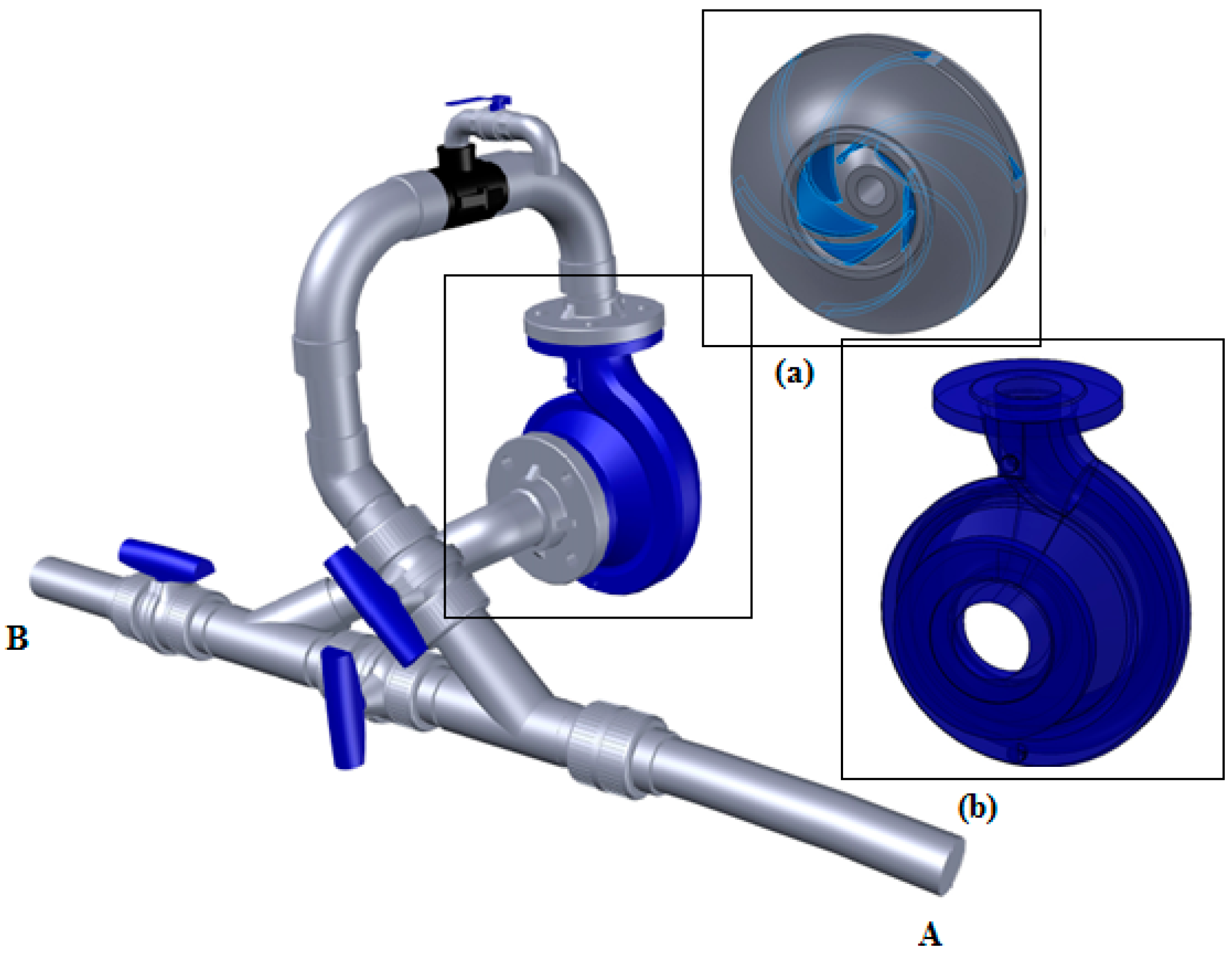
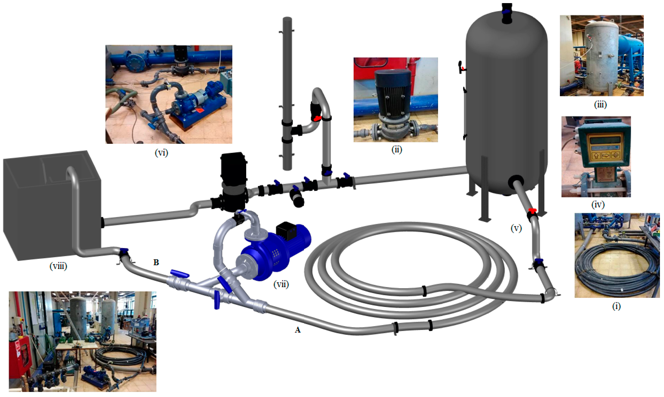
The hydraulic facility is composed of several components: (i) A loop high density polyethylene pipe (
Figure 1); (ii) a pump that feeds the loop pipe system; (iii) a compressed air vessel to stabilize the pipe system pressure; (iv) an electromagnetic flow meter to measure the instant flow; (v) flow control valves along the pipe; (vi) pressure transducers, to register the pressure variations and a picoscope data acquisition system connected to a laptop; (vii) a centrifugal micro PAT; (viii) a free surface reservoir, with a 90° triangular weir to calibrate the discharge flow. The nominal external diameter (DN) is 50 mm with 100 m of length. The pressure inside the air vessel can oscillate between 20 and 35 mWc (meters of water column).
Two pressure transducers are located upstream and downstream of the PAT, respectively at points A and B (
Figure 1). The best efficiency point (BEP) of the PAT is characterized by a flow rate of 3.36 L/s, with a head of 4 m, the efficiency of 60%, and the power of 80 W, for a rotational speed of 1020 rpm (
Table 1).
Due to the laboratory’s operational restrictions, the characteristic values of the PAT are limited. All tests were carried out for different steady state conditions depending on the opening degree of the flow control valves.
2.2. Experimental Tests
Several tests were carried out for different flow values and consequently different rotational speeds. Some tests are presented in
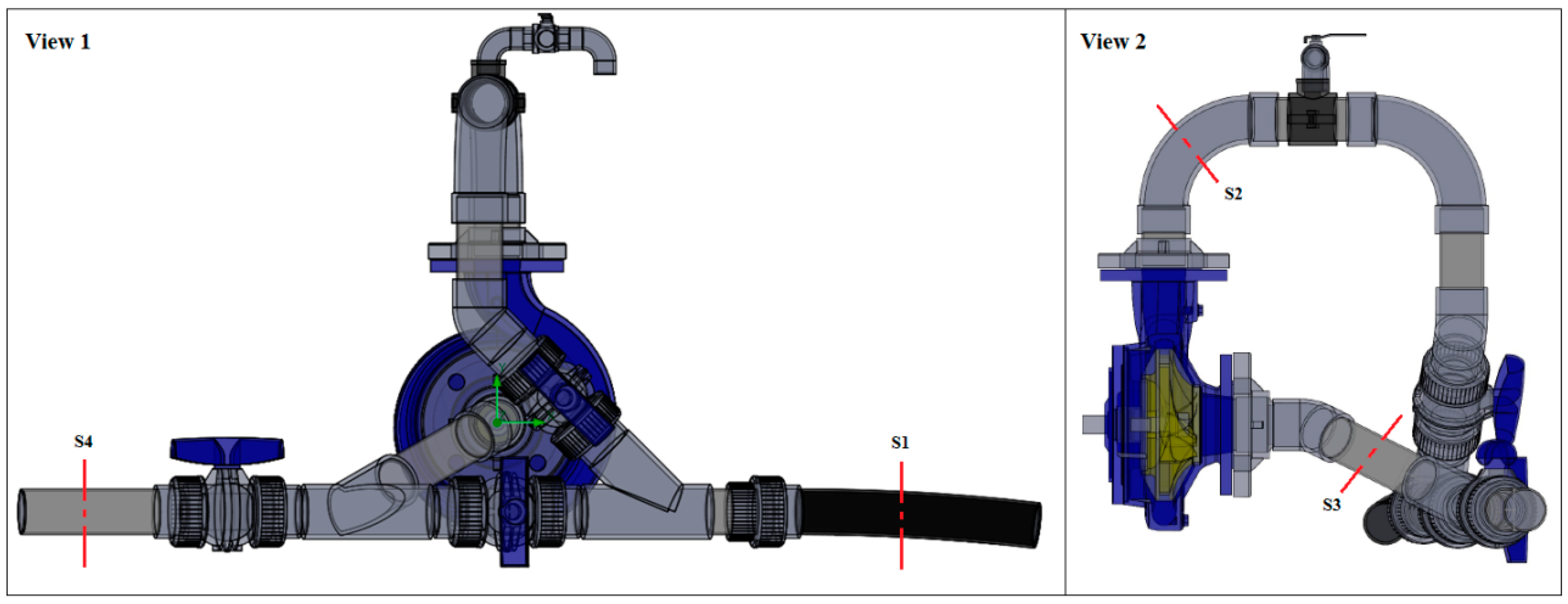
Table 2 sorted by the rotational speed values. For each flow rate the rotational speed of the PAT was measured by means of a digital tachometer. The pressure values were recorded as previously described, and the velocity profiles were collected in different PAT sections (S1–S4) using a 3000 series ultrasonic doppler velocimetry (UDV). This equipment allows the registration of velocity profiles, in real-time, either in steady or unsteady state conditions. This device is able to perform instantaneous measurements of fluid velocities at a number of points, along the direction of emission of the ultrasonic signal, with remarkably high resolutions in space and time. It is an interesting tool for turbulent flow analysis, where high spatial and temporal accuracies are required for both instantaneous measurements and averaging operations. In each UDV measurement, the velocity was captured in 100 different points in a total of 100 profiles. Details of the points (S1–S4) where the measurements took place are identified in
Figure 2.
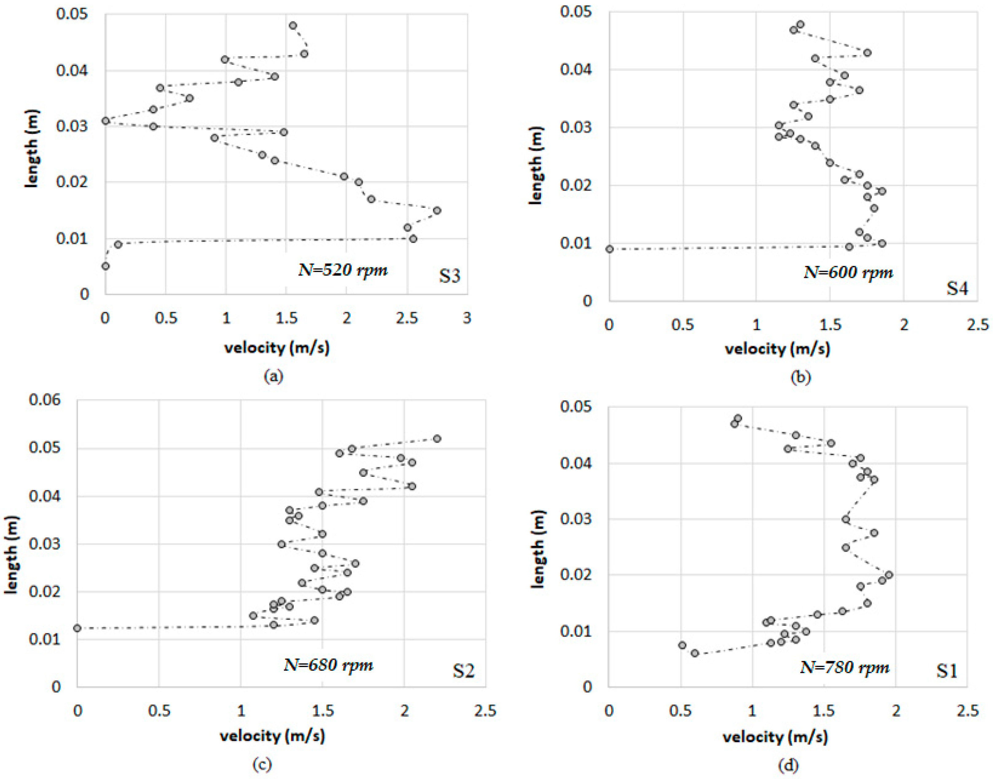
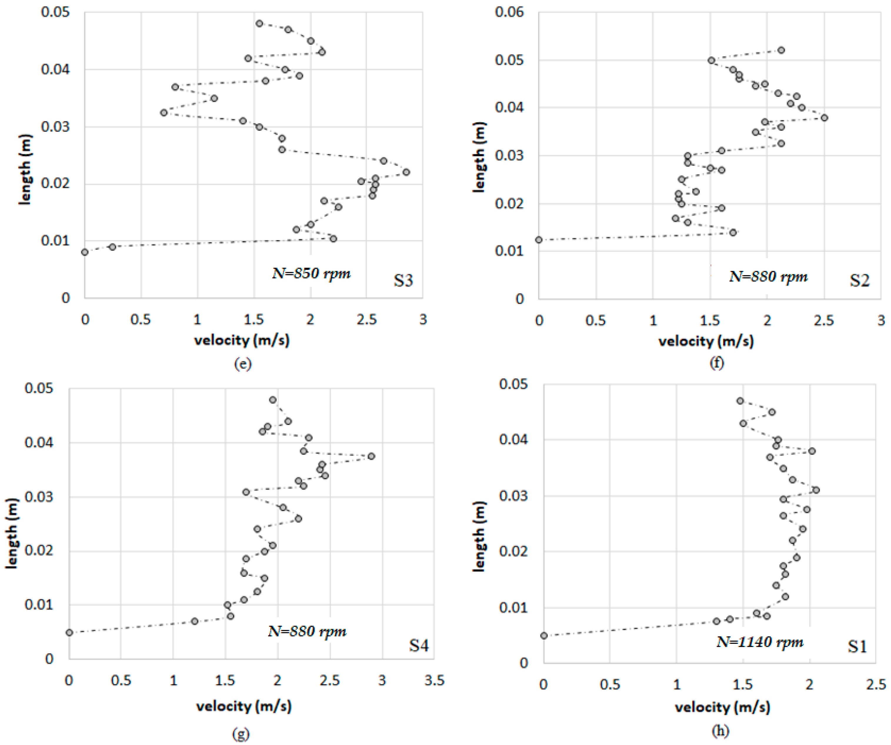
Figure 3a shows low velocity values in S3 at the draft tube induced by the existent vortex at the exit of the impeller. The influence of the curves in the inlet and outlet pipe to/from the PAT is visible in respective velocity profiles between S1 and S4 (
Figure 3a,c,e,f). In Section S1 the velocity profile is typical of a turbulent flow with a quasi-uniform velocity distribution, presenting only few fluctuations (
Figure 3d,h). The proximity of Section S1 to a 45° pipe branch also support this irregularity.
In order to collect the velocity profiles in Section S2, where the first velocity values were recorded by the extruder of the curve (
Figure 3c,f) with lower values, the influence of the curve in the non-symmetric velocity distribution is visible. The velocity variation for this measure point S2 results from the effect of the curvature, and also from the effect of the rotating flow from S1 to S2 due to the changes of the flow direction.
As a result of the rotational speed of the PAT and the shape of the blades, the flow has a rotational behavior at the outlet of the runner and along the draft tube, i.e., where the measured point S3 is located (
Figure 2). Thus, the flow leaves the impeller with a significant tangential velocity in relation to the axial one. From the exit of the runner and along the draft tube, a strong turbulent vortex is generated near the pipe’s axis, where the axial velocity of the flow is lower. In
Figure 3a,e, the low velocity values are close to the pipe’s axis, where the vortex core is located. Additionally, the velocity in the direction of the flow presents higher values from the axis to the periphery of the draft tube, since near the walls the rotation vorticity is significantly lower, enabling higher velocity values in the mean flow direction. The larger the cross-section of the draft tube occupied by the vortex, the greater the diametric length of the pipe (i.e., the axis-
y in
Figure 3a,e) where the lower velocity values are observed in the flow direction.
The axial velocity can be virtually blocked, in cases where the cross-sectional area of the draft tube, occupied by the vortex, is very significant. As a result of the rotational behavior of the flow and the reduced pressure values that occur at the draft tube, the resulting velocities are also reduced, which indicates an eventual reverse flow [
11].
In
Figure 3b,g, the measuring point S4 is already located out of the draft tube, so it is expected that in this section the vorticity and flow turbulence will decrease returning again to an approximate uniform flow type. The differential of velocities between the axis and the pipe wall in S4 is lower than in S3. The non-uniformity in the velocity distribution showed in
Figure 3b,g results from the vorticity that still attain S4, which also result from 45° junction of flow changed direction located immediately upstream (
Figure 2).
Most of the velocity profiles recorded show a strong reduction of the flow velocity in the adjacent area to the pipe walls, due to the tangential tension (drag tension) that occurs herein increasing the resistance to the flow propagation.
3. Numerical Simulations
3.1. Model Description
To perform the computational simulation of the flow inside the selected PAT, it was necessary to build the 3D geometric model represented in
Figure 4 based on the real PAT characteristics. For that, the geometry of the PAT was created in Solidworks and then imported to the CFD model (FloEFD). The geometric model resulted from gathering several independent solid components, with the most relevant parts (i.e., the impeller and the volute). The computational modeling was performed for the PAT system, between points A and B, located respectively upstream and downstream of the PAT (
Figure 4) being sections of connection to any water pipe system.
The elements used to support the construction of the impeller geometry of the PAT were as follows:
- ▪
Values of the characteristic parameters of the BEP of the PAT, supplied by the manufacturer and presented in
Table 1.
- ▪
Longitudinal and transversal sections of the PAT device, supplied by the manufacturer.
The simulations were performed considering an incompressible flow, with constant properties and using the
k-
ε model as the turbulent model. The flow inside the suction pipe is described by the Navier–Stokes–Reynolds Average for the
k-
ε model [
12]:
where
is the effective viscosity for turbulence,
is the sum of forces, and
is the modified pressure given by [
13]:
k-ε model assumes that the turbulent viscosity is related to the turbulent kinetic energy and dissipation through the relation:
The values of
k and
ε come directly from the transport equations for turbulent kinetic energy and dissipation range of turbulence [
14]:
where
, and
,
and
are constants and
is the production of turbulence due to the forces of viscosity which is modeled as follows [
13]:
For an incompressible flow,
is small, and the second term on the right does not contribute significantly [
14].
3.2. Mesh
After defining and bringing in the geometric model, an automatic generation of the initial calculation mesh was conducted, by specifying values for the parameters used to control the mesh resolution. These parameters need to be adequate to the characteristics of the geometric models to obtain results with a satisfactory level of accuracy, without using significant computational resources. Considering the complexity of the rotor geometry, it is advantageous to refine the cells in the local region of the computational domain relative to the rotor, using the definition of an initial local mesh [
15].
The mesh generation process begins with the definition of the rectangular computational domain. Three sets of orthogonal planes to the Cartesian coordinate system were defined inside of it. The intersection of these planes defines the set of rectangular cells that form the base mesh. In the next stage of the process, the geometry inside the computational domain, i.e., the PAT system, is captured [
16]. The program crosses the mesh cells sequentially and for each cell it parses the geometrical configuration inside the cell. Followed by a refinement criterion:
- ▪
If
, the cell has to be subdivided. The value of indicator
(i.e., refinement indicator value) is calculated individually for each cell according to an algorithm that controls the type of refinement. The value of
is a constant, defined automatically and represents the refinement threshold value. Setting refinement levels individually for each criterion makes it possible to influence the total number of cells that will be generated [
15].
Additionally, the refinement level of the cell is the number of times it has been refined relative to the initial cell in the base mesh. In SolidWorks Flow Simulation the maximum number of refinement levels is limited to seven, so that the smallest cell size is 1/128 of the original cell in the base mesh (level 0) [
16].
An initial mesh that best fits the geometric model is obtained, leading to results that more accurately translate the flow dynamics. The values for the parameters that govern the procedure of the CFD model were defined for the automatic generation of the initial local calculation mesh, according to [
15]. The CFD model automatically specifies the remaining parameters that govern the initial, local and global mesh generation. Since the flow field inside the PAT presents significant complexity induced by the rotational movement of the rotor and the associated geometry, the initial calculation mesh was also refined. Hence, different values were allocated to the parameters that govern the procedure of the CFD model, for the initial calculation mesh, to the solution during the calculation process.
To ensure a proper and acceptable accuracy of the results, the discretization mesh undergo a Mesh Sensitivity Analysis (MSA), in which the density of cells is gradually increased and the solution must be re-assessed until results demonstrate sufficient independence on the mesh size [
16]. The discretization of the mesh was performed by assuming an initial coarse mesh with the total number of cells equal to 25,668, followed by a mesh refinement process. This process stopped when the difference in the head drop (i.e., in point B) between consecutive meshes was less than 1%, which occurred for mesh with 102,274 cells (
Table 3).
3.3. Computational Fluid Dynamics (CFD) Results
In the CFD model, the boundary conditions were consigned to sections A and B (
Table 2), as the inlet and outlet measured points of the PAT system, respectively. The volume of the flow rate, corresponding to each test, was allocated to the inlet condition. As for the outlet condition, the pressure recorded in the transducer, obtained at point B, was set. For the rotation of the impeller, the corresponding rotational speed obtained experimentally was also considered.
Table 4 shows the operating and boundary conditions given to each of the tests and the respective numerical results.
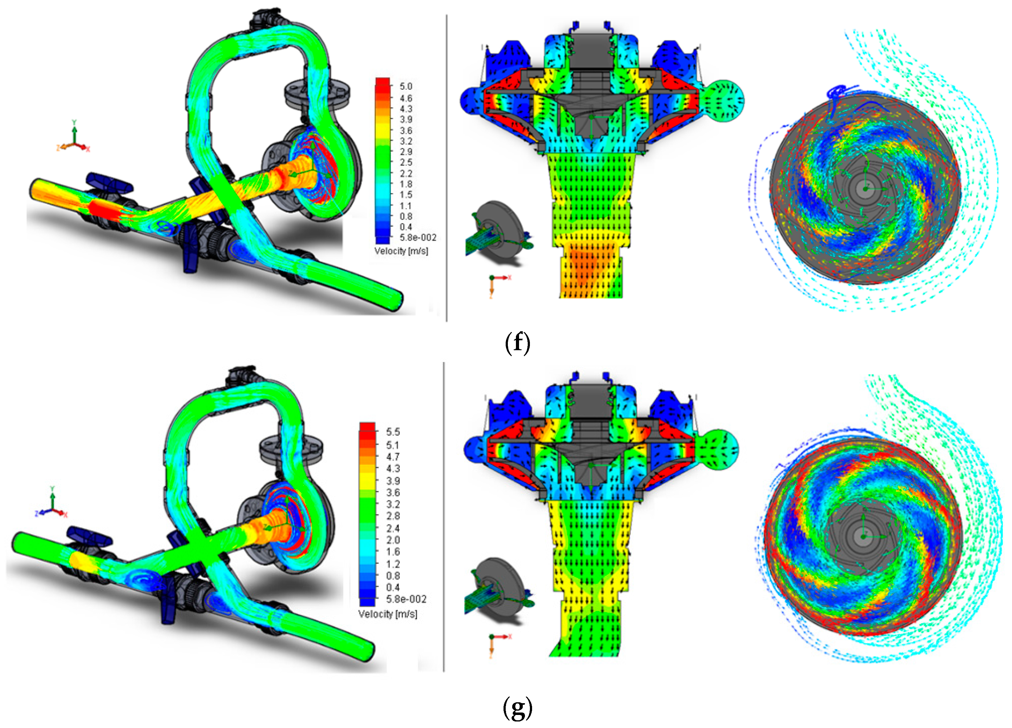
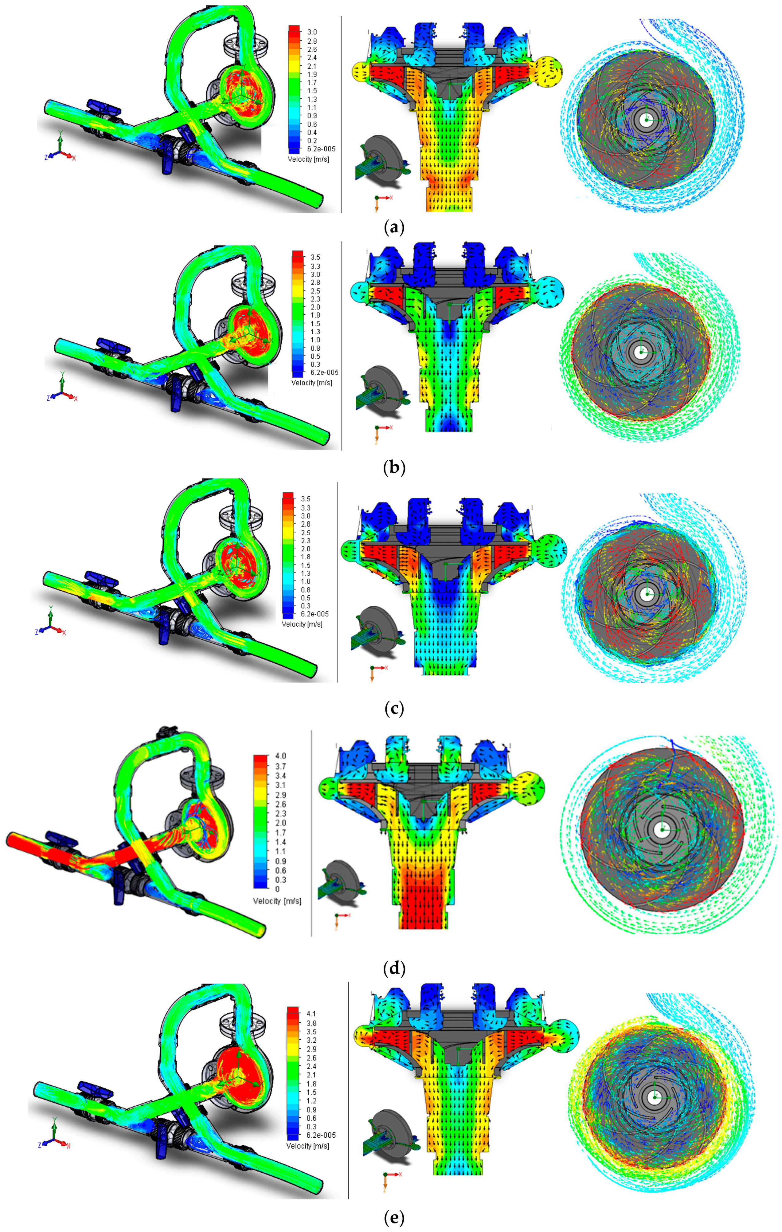
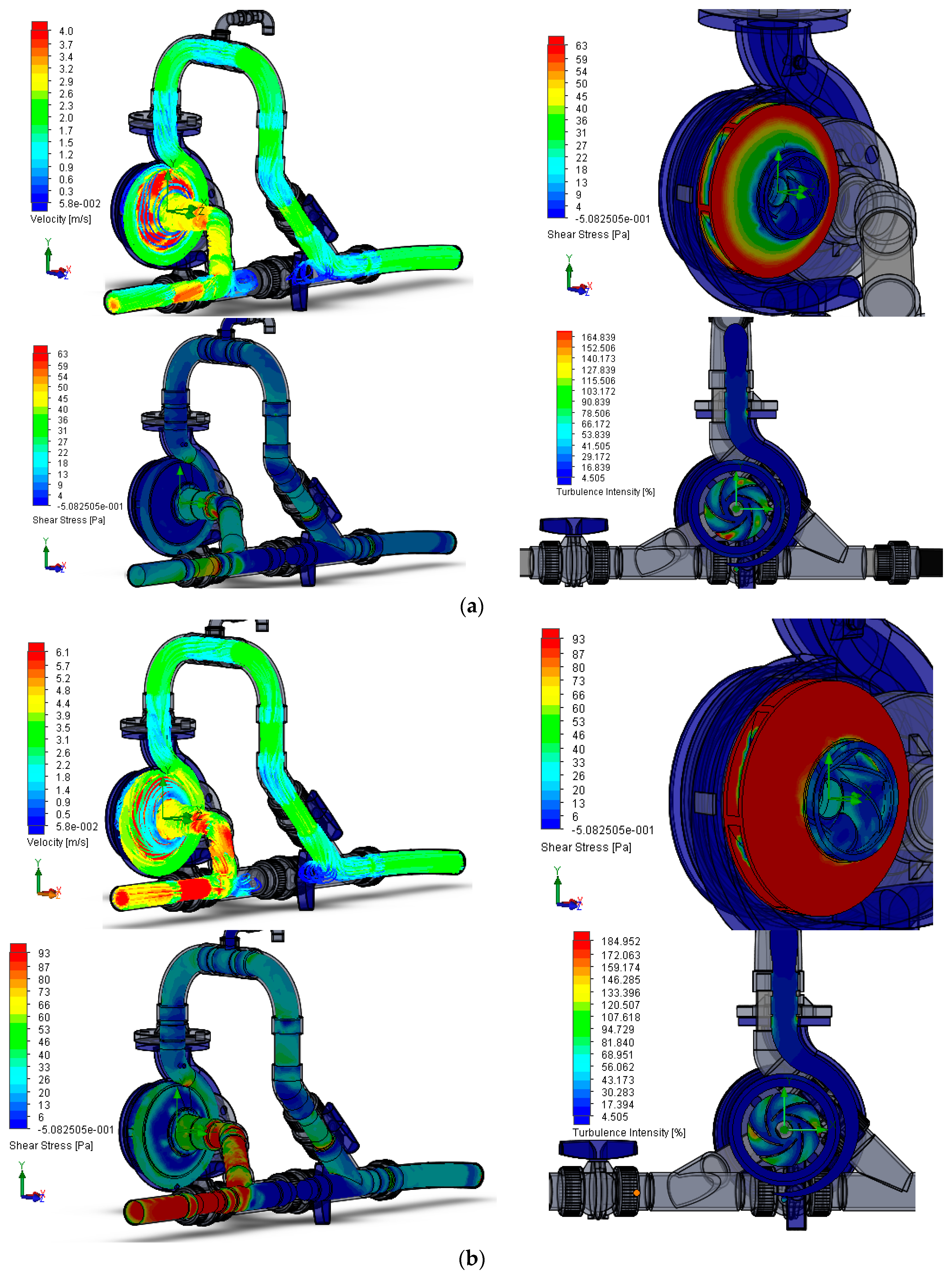
Figure 5 shows the velocity streamlines and the velocities field in planes that intersect the geometric model. The hydrodynamic of the flow that occurs near point B is characterized by the presence of curves and elbows at upstream. This figure shows a reduction in the velocity magnitude, upstream and along the impeller, caused by the energy promoted by the flow to the impeller. The vortex that forms at the exit of the rotor and that extends downstream thereof is associated with turbulence, and hydrodynamic instability, which effects result in pressure fluctuations and efficiency losses.
In
Figure 5, the velocity streamlines distribution confirms the rotation of the flow along the draft tube, and the distribution of the tangential velocity shows increasing values from the axis to the wall surface of the pipe. The reduced flow velocity values that occurred in the vortex core (located near the axis of the pipe) that is formed downstream of the rotor, and the marked velocity that reaches the wall of the draft tube due to the rotationally of the flow, are more visible in
Figure 5d,f,g. The rotational behavior, affected by the rotational speed of the impeller and the shape of the blades is also verified. A decrease of the tangential velocity values from the periphery to the shaft of the runner confirming the centrifugal force effect is shown which arises with the rotor rotation increase. The flow enters the volute and exerts a radial force on the rotor, thereby imparting a certain rotational speed to the impeller. Consequently, the runner rotation continuously varying the direction of flow along the impeller, becomes to axial direction at the exit.
The results show that for the same number of velocity vectors, and as the speed ratio increases, high concentration of velocity vectors migrates from the outside of the blade to the core side. The complex flow near the impeller inlet varies with the rotation, inducing different performances. Hence, the complex vortices cause additional vibrations, turbulences and consequently additional dissipative effects [
17,
18].
4. Experimental and Computational Fluid Dynamics (CFD) Comparisons
4.1. Velocity Profiles
Experimental tests were used to calibrate and validate the CFD model. Therefore, the hydrodynamic of the flow inside the PAT was simulated for the same operating conditions as the lab conditions, according to the following methodology: (1) Obtaining the distribution of physical parameters describing the hydrodynamic of the flow in planes that intersect the representative geometric model of the PAT; (2) recording the velocity variation in the measured points where the velocity profiles were recorded in the direction of the UDV velocity values; (3) comparing the velocity profiles between experimental tests and the numerical simulations.
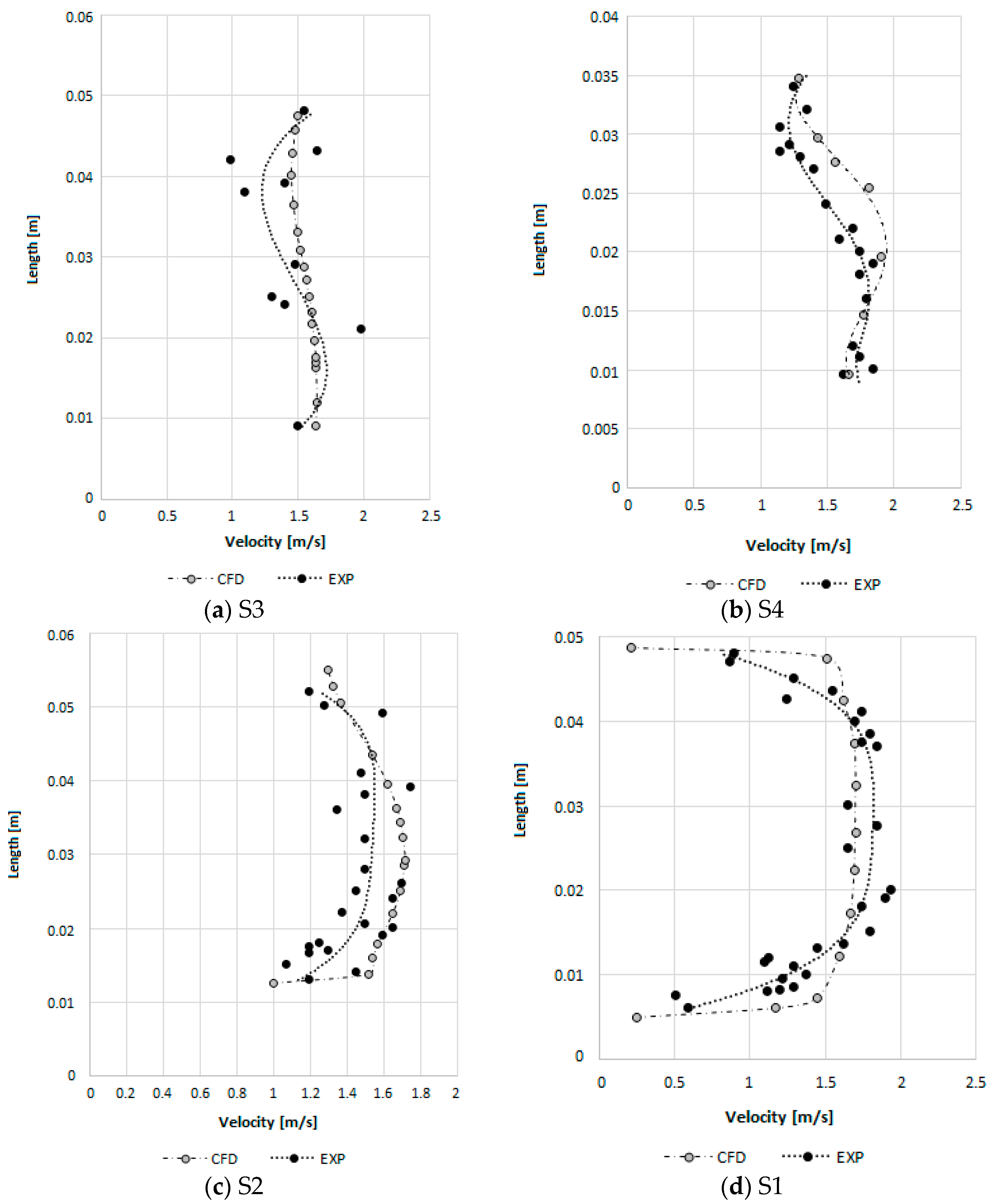
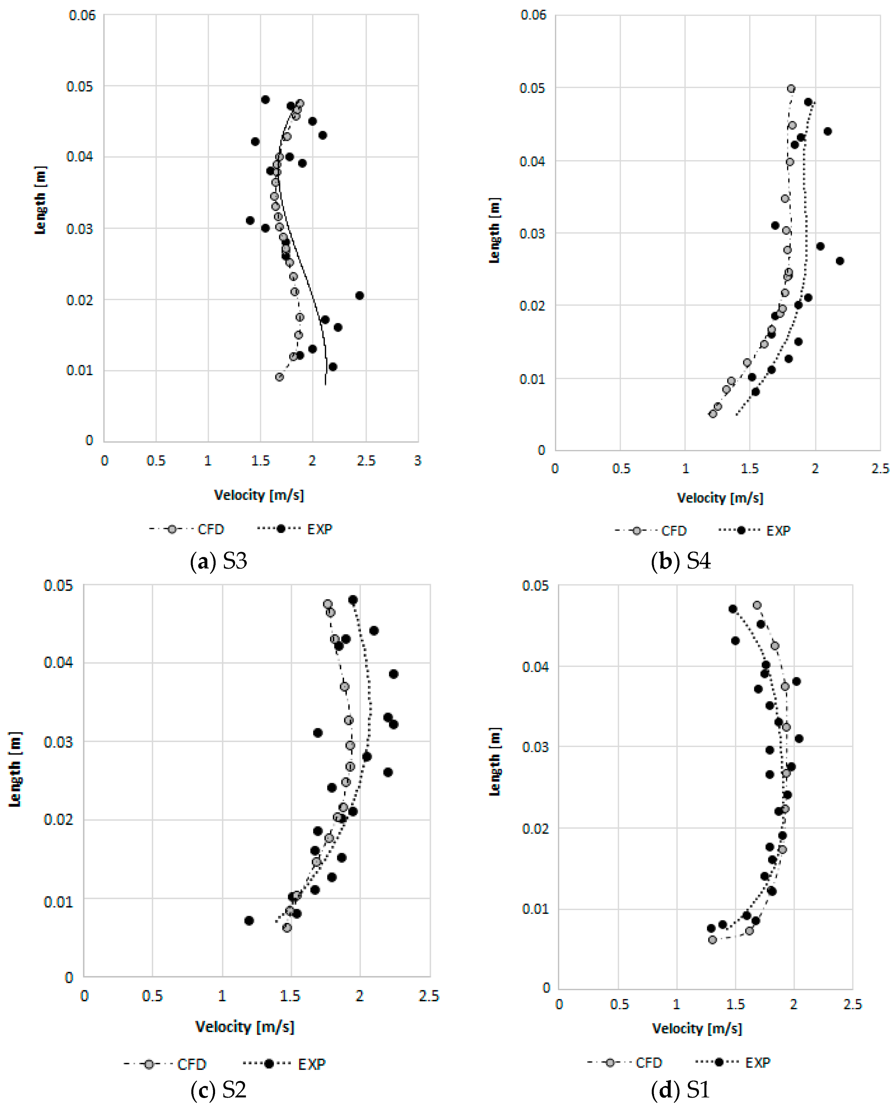
From the computational simulation for different rotation speeds, the velocity profiles were obtained in the four measure points (
Figure 6). Compared with the experimental velocity profile, the CFD model shows a trend of velocity variation similar to the one observed with UDV. Since the variation of the physical parameters that characterizes the hydrodynamics of the flow inside any hydraulic device depends on the geometry, it is necessary to adequately simulate the shape of the device. Thus, the major differences can be related to the limited data to perform the geometry of the PAT installation.
Figure 6 shows some irregularities in the distribution of velocity values. Both velocity profiles are typical of turbulent flows.
Due to the proximity of S3 to the turbulent flow in the PAT rotor (see
Figure 2), an irregular velocity distribution is expected in this section (
Figure 6a). The experimental velocities profile shows this expected irregularity noticeably, and the CFD results also allow the identification of the typical flow pattern of the draft tube flow. The mean velocity values relative to the velocity diagrams obtained experimentally and computationally are 1.43 m/s and 1.49 m/s respectively for values of the flow around 2.4 L/s. Thus, the difference in the mean velocity between experiments and simulations are quite similar.
In
Figure 7, for higher rotational speed values the behavior is similar. Additionally, the non-uniform velocity distribution is visible due to change of direction of the pipe flow. The velocity is affected by the viscous tangential stresses occurred near the pipe wall. Thus, the velocity distribution that was obtained through the CFD model shows the same tendency of the measured flow behavior verified in the experimental setup. The mean velocity values relative to the velocity distribution obtained experimentally and by numerical simulation were 1.87 m/s and 1.83 m/s respectively for a mean flow of 3 L/s.
The results for the target operating conditions are summarized in
Table 5. The results show good correlation between the experimental data and the CFD model. The main discrepancy was encountered for the torque measurement predictions, since the CFD overestimate the torque extracted by the turbine, and consequently the turbine efficiency, since the scale effects are not possible to reproduce with the CFD model. This overestimation is caused by the bearing losses, which are not modeled in the CFD analyses. The total estimated bearing losses represented about 11.36% of the discrepancy (in average) in the shaft power between the experimental data and the numerical predictions, as in previous research suggested by [
17].
The efficiency values present the same range between 30% and 60% both for low (<850) or high (>850) rotational speed values.
4.2. Triangle of Velocities
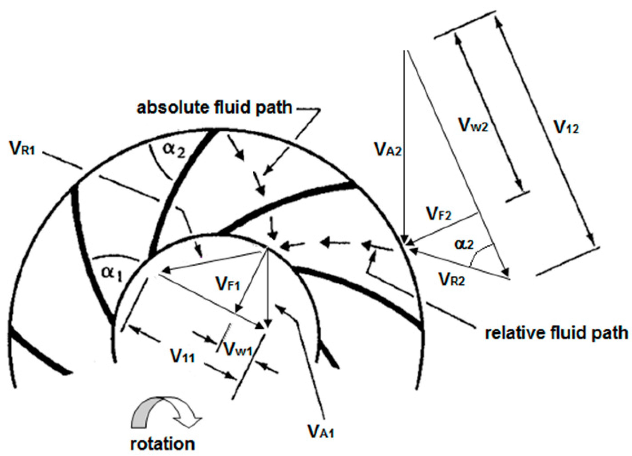
The distribution of the velocity vectors as the flow enters and leaves the impeller in a PAT (
Figure 8) is studied as a fluid structure interaction problem between static and movable parts [
19,
20,
21]. The velocity vectors of a PAT can be decomposed into: (a)The absolute velocity
of the flow at a point, i.e., the velocity relative to a stationary point at radius
r; (b) and the relative velocity of the flow
, i.e., the velocity of the fluid relative to the impeller.
and
are the tangential and the radial components of
, respectively.
is the peripheral velocity of the impeller itself, at radius
r with rotational speed
n. The subscripts 1 and 2 represent the inlet and outlet of the impeller, respectively.
To design the velocity vectors, it is assumed that the flow passes through the impeller, and the relative velocity traces a path which is everywhere congruent to the blade, according to [
22,
23,
24,
25]. At any radius r in the impeller, the flow describes a tangential component of velocity
, corresponding to a tangential momentum
. The moment of this flux to the impeller axis is
. The torque change of moment flux between radius (entrance impeller radius)
r1 and (exit impeller radius)
r2, respectively the [
26]:
The flow across a runner is characterized by the three types of velocities (i.e., the absolute velocity of the water (
V), the relative velocity (
W) guided by the blades orientation and the tangential velocity (
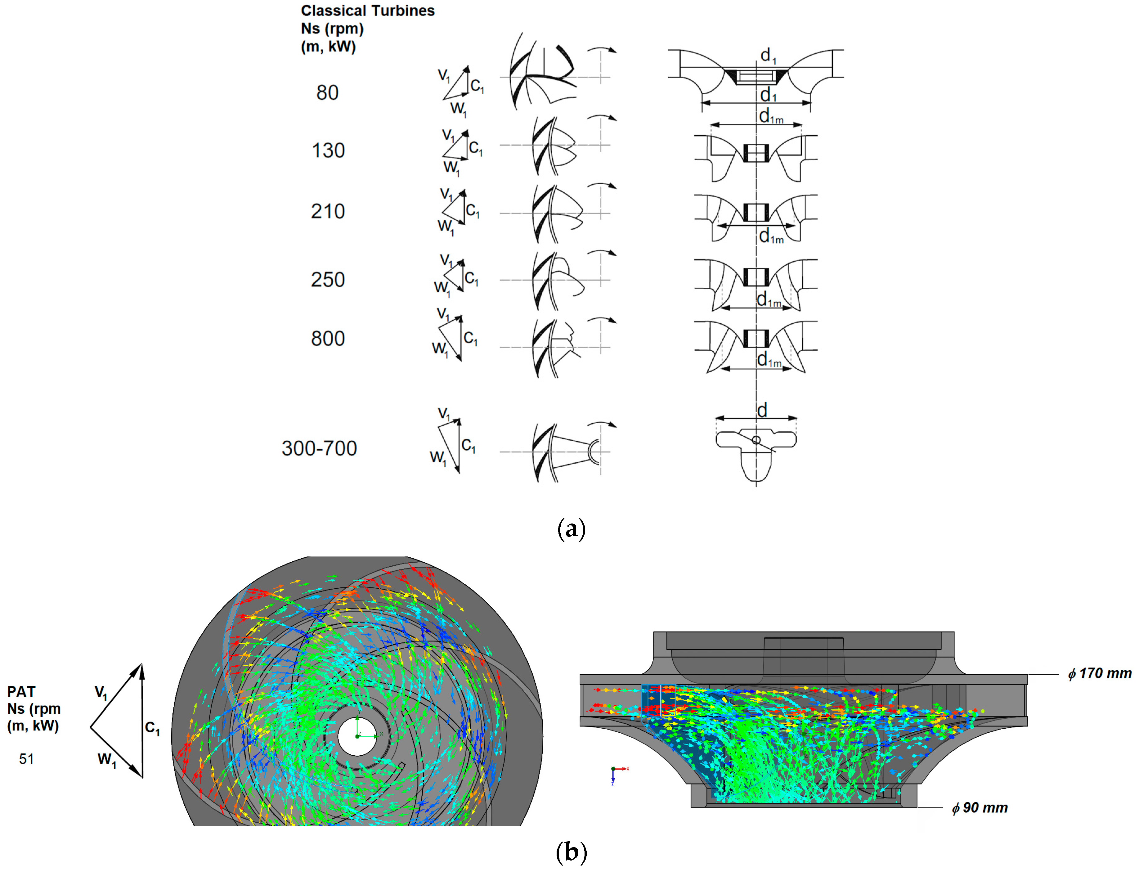
C) imposed by the rotation of the impeller, a comparison with classical turbines velocity triangles at inlet of the impeller (
Figure 9a), with the studied PAT, is visible the differences in the peripheral velocity due to the smaller inertia of the PAT and the PAT blades configuration. This difference is responsible for a lower efficiency value of PATs against the lower specific speeds Francis turbines. This difference will affect the dynamic behavior of both machines.
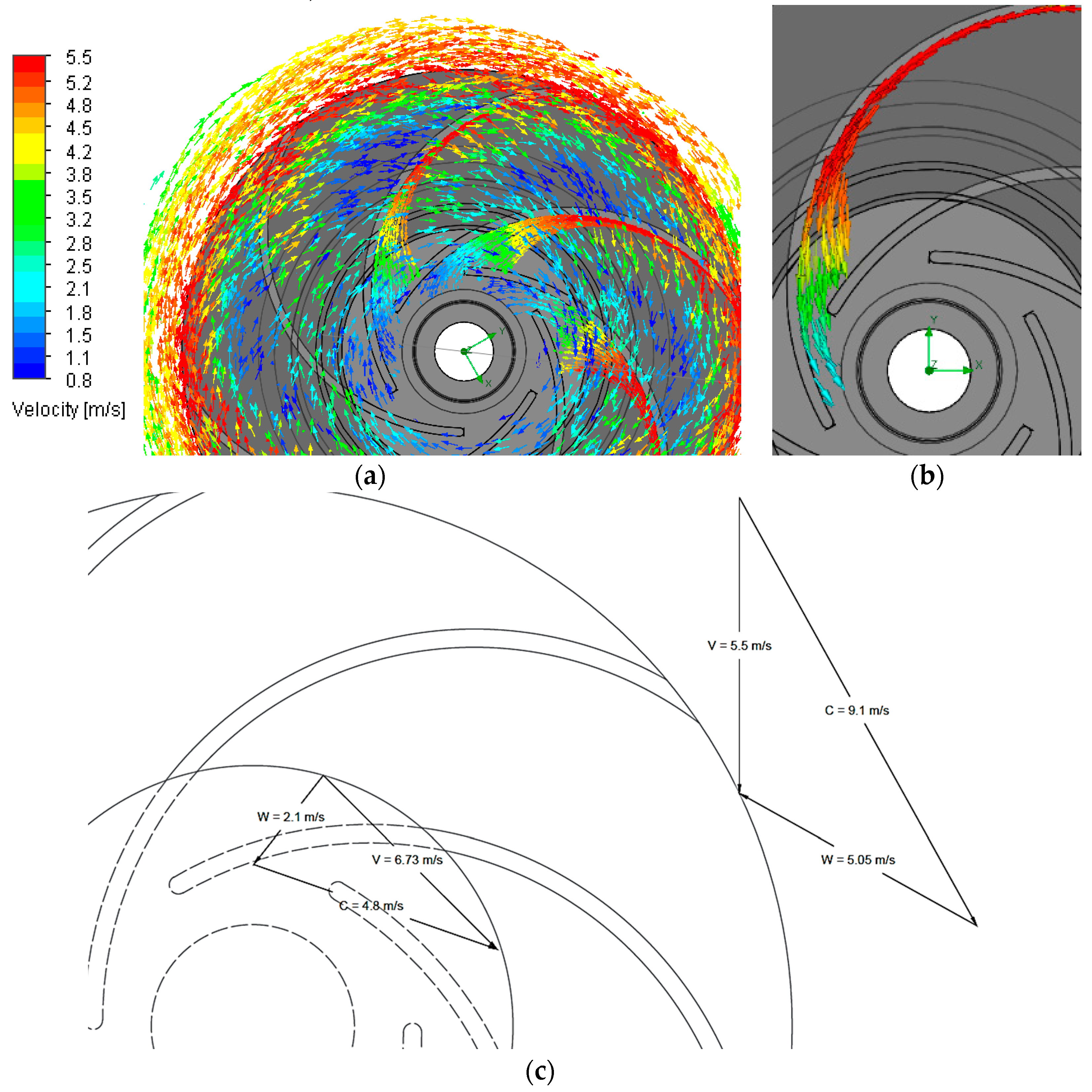
Analyzing the velocities field of the flow in the radial PAT impeller the
V and
C components at each particle position are visible (
Figure 9b). The inlet and outlet velocity vectors of
V and
W components can be observed in
Figure 10a,b.
According to the CFD results, the inlet and outlet triangle of velocities in the PAT is also obtained giving information about the momentum and the rotation effect of the fluid at the impeller entrance and exit.
4.3. Dissipative Effects
Patterns of wall shear stress (WSS) influence the progression of the flow resistance. WSS, defined as the tangential force imposed on the pipe or device wall by the flow, plays an important role in the dissipation effects. Furthermore, extremely high values of WSS are associated with fluid structure interface interaction [
21] responsible for the resistance to the flow progression and for wear of material inducing friction, separation zones, pressure variation associated to the velocity exchange, visible in the path lines, towards to initial erosion process. In a fully developed steady uniform regime, the equilibrium of forces shows that the average wall shear stress is related to the friction slope. When the accelerations are too great for the quasi-steady hypothesis to be used, the instantaneous value of the wall shear stress,
τw, requires a more precise evaluation, considering the effects of the variation in time of the velocity fields. Hence the analyses used the 3D velocities and the Reynolds stress values by using the CFD model coupled
k-
ε turbulence model.
The turbulence model used in this study is the robust and well known realizable
k-
e model. The term realizable means that the model satisfies certain mathematical constraints of the Reynolds stresses, consistent with the physics of turbulent flows. In comparison to the standard
k-
e model, the realizable
k-
e contains an alternative formulation for the turbulent kinetic energy, and a modified transport equation for the dissipation rate, that has been derived from an exact equation for the transport of the mean-square vorticity fluctuation. In the current study, a rotor–stator simulation is performed with the entire turbine assembly. The flow prediction in the impeller and draft tube is sensitive to the boundary conditions applied and the turbulence model selected. Swirl plays a vital role in the transformation of kinetic energy into pressure energy essentially in the draft tube, preventing the flow separation at the cone wall. The CFD results fit well with the UDV measurements (see
Figure 6 and
Figure 7) along the PAT system for the all turbulence used model. In the present rotor–stator simulation, the entire turbine flow domain was used.
The small wakes due to the counter rotating below the runner due to the blade-hub clearances, or the flow jet coming out of the blade-hub with high velocity, are captured in the CFD simulations. However, flows with a strong streamline curvature that happens in curves, in the interaction rotor–stator, and in the draft tube need special concerns since the model can present some inability to characterize all the real effects.
Figure 11 presents the swirling strength of the vortex core region at the impeller exit in the draft tube and in all flow direction changes.
In order to analyze the effect of the jets, the velocity and turbulent quantities were observed from the simulations at the impeller-draft tube interface. A separation tendency appears on the rotor–stator interface and on impeller-draft tube transition. The circumferential distribution of the energy affects the flow near the runner increasing the turbulence and associated dissipative effects. The radial wall-shear stress is presented. Higher wall-shear stress is obtained locally in the out surfaces of the impeller. The flow is completely attached until the end of the runner. The high-velocity jets in pipe curves and the draft tube create a lower pressure region. The lower pressure allows bending the streamlines toward the swirl, despite the centrifugal force imposed to the fluid in the impeller and at the transition to the draft tube. The CFD model accounts for the effect of the rapid strain, the strong streamline curvature and the swirling motion (vorticity), which are visible in the simulation results.
5. Characteristic Curves
The specific speed plays an important role for selecting the type of turbine. It is a quantity derived from dimensional analysis, defined as the speed of a turbine which is identical in shape, geometrical size, blade angles, with the actual turbine, but of such a size that it will develop unit horse power when working under a unit head [
11,
12,
13,
14,
22,
27,
28]. The main characteristic parameters of a turbo-machine can be converted into non-dimensional parameters, such as:
where
H (m),
N (rpm),
Q (m
3/s),
P (kW) and
D (m) are the head, rotational speed, flow rate, power, and impeller diameter respectively.
Therefore,
is a characteristic parameter [
19] concerning the turbine type, the runner shape and its associated dynamic behavior. According to [
17,
18] and [
23,
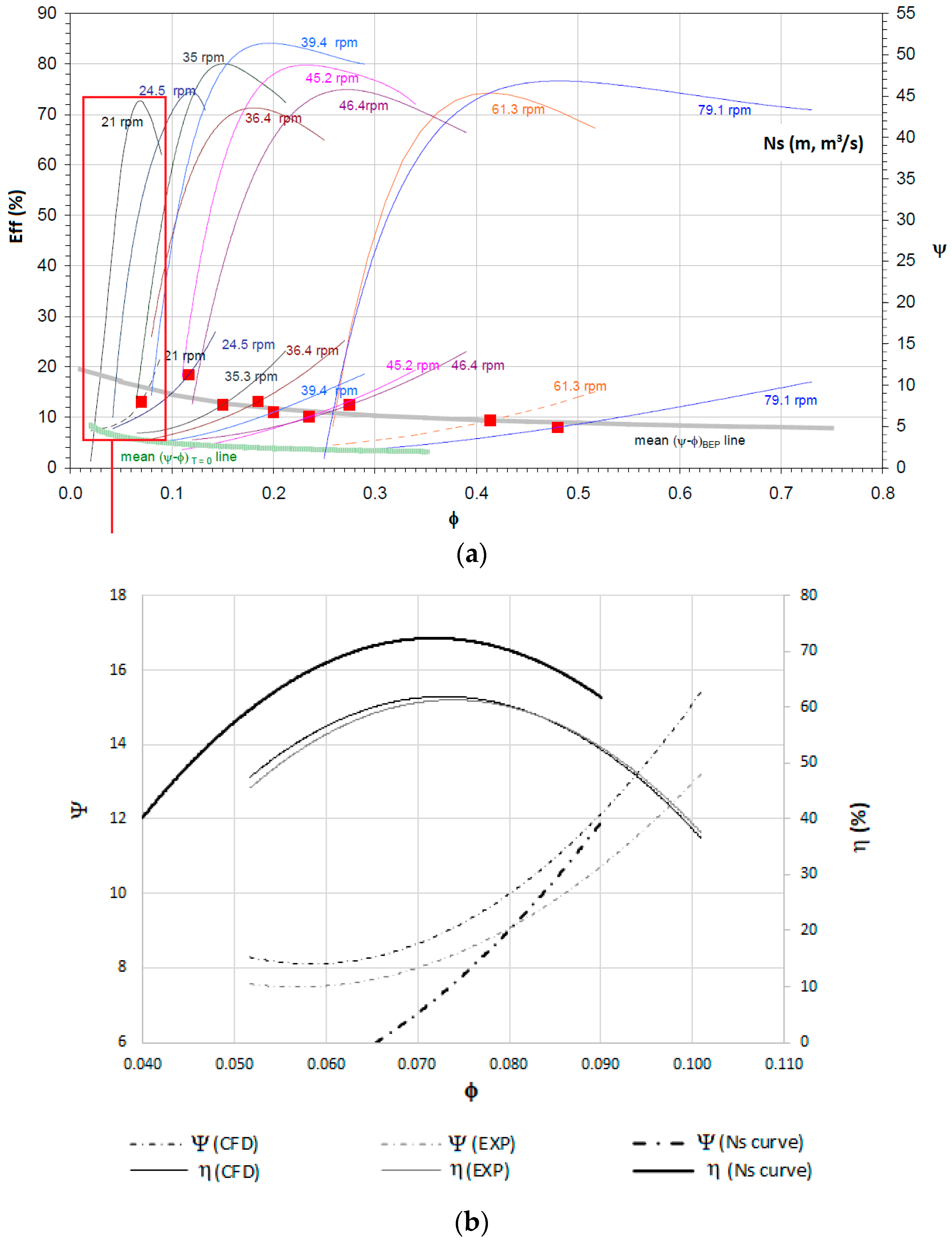
29] the performance characteristics of 9 PATs with different specific speeds (
Ns) were considered (
Figure 12a), namely for different specific speeds (i.e., 21 rpm, 24.5 rpm, 35 rpm, 36.4 rpm, 39.4 rpm, 45.2 rpm, 46.4 rpm, 61.3 rpm and 79.1 rpm).
Figure 12a is representative of different PATs tested in laboratory [
26,
30,
31,
32]. Knowing the specific speed of the analyzed PAT at IST, which is 21 rpm (n, m
3/s) or 51 rpm (m, kW), with a nominal rotation speed of 1020 rpm, a comparison is made with the available Ns curves of available PATs. The maximum efficiency obtained for the PAT at IST and by the CFD model was below than 70%, due to the additional turbulence between rotor and stator edges inducing small leaks, and due to the micro scale of the small PAT turn this effects predominant, reducing the efficiency of the machine.
Figure 12b,c present comparisons between CFD, experimental for the tested PAT and with the Ns available curve in (a).
6. Conclusions
Experimental and CFD simulations were performed for detailed flow analysis to study the velocity variation in a PAT with the specific speed of 21 rpm (m, m3/s). For the velocity profiles analysis, a UDV 3000 series technique was performed. Despite the difficulty of the probe access and the complexity of the instrumentation adjustment, the flow field in the region of the PAT was characterized. The obtained experimental data and CFD results allowed to understand the flow behavior along the PAT, inside the volute, crossing the impeller, in the draft tube, and, most interesting, was the analysis of the velocity vectors along the blades for different operating conditions associated to each flow discharge, head and rotational speed. The obtained data provides a good base for better characterizations the best flow conditions, the main loss mechanisms through the velocity fields between the rotating and static parts of a runner. The analysis to the velocity fields of the flow in the radial PAT impeller allowed the characterization of the triangle of velocity components (i.e., V, W, C) at each particle position at inlet and outlet of the impeller. From the CFD simulation and for different rotational speeds, the velocity profiles were obtained in different measured points of the PAT. The velocity profiles from CFD simulations show a trend of the velocity variation similar to the one observed with the UDV in the experimental facility. Since the variation of the physical parameters that characterizes the hydrodynamic of the flow inside any hydraulic turbo-machine, adequate shape of the impeller was then imposed.
CFD analyses allowed the estimation not only the triangle of velocities at inlet and outlet of the PAT impeller, but also the effect of the blades’ orientation, the rotational flow at the draft tube, which induces additional efficiency losses in the PAT system, when compared with classical turbines which are geometrically more adequate to this flow direction.
Analyzing the differences in individual quantities impacting efficiency leads to the conclusion that the largest disparity is due to differences in computed and measured torque (or shaft power) on the PAT shaft. All the computed variants yielded values of torque significantly higher than the value actually measured. The difference ranges from as little as 3% to a whopping 40%. As a result of the torque overestimation, the numerical simulation also foresaw the turbine efficiency as a function of the configuration of the velocity triangles. Aside from mechanical losses, other factors that can cause the torque discrepancy are small geometry differences between CAD and the real PAT, most significantly through the scale effect of frictions and bearings, the surface roughness of the test model (since CFD analyses were performed with hydraulically smooth surfaces), eventually entrapped air micro bubbles in the pipe loop and inside the PAT, carrying additional turbulence and swirl effects. The scale effects namely friction, bearings and flow impact, flow separation and vortex may cause the torque calculation inaccuracy in the numerical simulation, which lead to the numerical efficiency greater than the experimental data. The majority of the momentum losses (~12%) is induced by bends, the inlet and outlet of the impeller, along the blades, and the change of flow direction due to the viscous drag on these surfaces, inducing rotational flow characteristics with additional instability. A rotor–stator simulation was performed showing swirls due to the transformation of the kinetic energy into pressure. The swirling strength of the vortex core region at the transition from the impeller to the draft tube and in all flow direction changes induce dissipative effects occurred in this PAT system. The circumferential distribution of the energy affects the flow near the impeller, increasing the turbulence and consequently the associate head loss effects. An effort should be done to minimize the losses due to the shear stress, turbulence, and leaks with specific jets and rotating flow and vortex formation in PATs. Nevertheless, the overall predicted torque is relatively accurate for the turbulent model tested with an increase in the accuracy upon successive grid refinements.
Overall, the selection of a suitable turbulence model is of paramount importance regarding the accuracy of expected results. Under such circumstances, the choice must be guided by computer experience, parameters of the generated mesh, and the boundary (initial) conditions being set.

 ,
, 


