Article

Haematocrit Distribution in Coronary Arteries: A ROM-PINN and Data-Driven Approach for Predicting Multiphase Flow

Department of Mechanical Engineering, University of Birmingham, Birmingham B15 2TT, UK
*
Author to whom correspondence should be addressed.
Fluids 2026, 11(5), 118; https://doi.org/10.3390/fluids11050118
Submission received: 25 March 2026 / Revised: 6 May 2026 / Accepted: 11 May 2026 / Published: 14 May 2026
(This article belongs to the Special Issue Advances in Hemodynamics and Related Biological Flows, 2nd Edition)

Abstract

Blood is a multiphase fluid, constituted of a plasma phase and a red blood cell (RBC) phase. Predicting the distribution of the RBC phase has applications in terms of medical device design, and for the characterisation of the risk of thrombus formation where atherosclerosis is present on coronary arteries. Computational fluid dynamics (CFD) can be used to simulate the multiphase flow of blood, but is time-consuming and requires a high level of technical expertise. This study evaluates the use of artificial neural networks (ANNs), as an alternative to CFD, to predict RBC distribution as part of blood flow through a coronary artery bifurcation model, both including and excluding stenosis. ANNs were trained on a dataset of 80 simulations generated using steady-state multiphase CFD. The initial data-driven ANNs encountered issues with overfitting and high errors in velocity component predictions. A physics-informed neural network (PINN) was employed, using a reduced order model (ROM), to enhance velocity component predictions, achieving average percentage error (APE) within 8.5% of CFD. These improved predictions were integrated into a hybrid model combining the PINN and the data-driven ANN to predict RBC distribution more effectively. The hybrid model achieved APEs ranging from 0.04% to 0.05%. Moreover, the hybrid model’s predictions were 14 times faster than CFD transient runs, demonstrating potential for translation into clinical use. In conclusion, a combined ROM-PINN and data-driven approach enables fast high-accuracy predictions of flow for multiphase fluids such as blood when compared to CFD.

1. Introduction

Atherosclerosis, the development of fatty plaques within the artery wall, is associated with regions of low wall shear stress [1], and is the leading cause of mortality worldwide, contributing heavily to cardiovascular disease [2,3]. Coronary atherosclerosis is the primary catalyst for plaque disruption with superimposed thrombosis, which is the main cause of acute coronary syndromes such as myocardial infarction [4]. In detail, the left main coronary artery has a bifurcation, with two ‘daughter’ arteries which are the left anterior descending and left circumflex arteries. Typically, atherosclerosis occurs towards bifurcations [5], as well as downstream from a region afflicted with stenosis [6] as caused by fatty deposits during atherosclerosis.
Non-invasive techniques such as Doppler-based echocardiography enable assessment of the coronary vasculature and micro-vasculature [7]. However, whilst good at imaging transient flow, Doppler techniques are limited in their ability to visualise full flow fields. More comprehensive flow imaging is feasible via 4D flow magnetic resonance imaging (MRI), enabling patient-specific analysis; however, 4D-MRI is not readily available, and scans are time-consuming and costly [8]. Other techniques can be used to evaluate blood-flow patterns, but all with limitations. For example, a pulmonary artery catheter can be used, but this is invasive and lacks specificity [9]. It poses risks such as catheter-related sepsis without offering a comprehensive view of blood flow [10]. Lab-based techniques, such as Particle Image Velocimetry, can also be employed [11], but timeliness for clinical assessment is limited. A non-invasive alternative is the use of computational fluid dynamics (CFD) which enables a comprehensive haemodynamic assessment [12,13]. It is currently the only method by which to predict haematocrit distribution when analysing blood flow [14]; briefly, this is how red blood cells (RBCs) are distributed in blood within the cardiovascular structures and has implications for thrombus formation.
CFD modelling of blood is complex because of blood’s constitutive make-up. Blood is a multiphase fluid primarily constituted of plasma and formed cells. Plasma behaves as a Newtonian fluid, it is composed of 90% water with the rest being proteins and solutes. Red blood cells (RBCs) represent over 99% of cellular volume fraction [15]. Haematocrit is defined as RBC volume concentration, which for healthy males is reported to range between 41 and 50% and for healthy females between 36 and 44% [16,17]. Studies of animal models of human blood typically use inclusion criteria such as systemic haematocrit of at least 45% to enable human blood viscosity to be appropriately mimicked [18].
CFD can be used to predict regions at risk of thrombus formation [14,19]. For instance, regions where RBCs are exposed to low shear are at increased risk of thrombus formation. RBCs also influence platelet movement [19]. During arterial thrombosis, elevated haematocrit enhances platelet accumulation at the site of vessel injury [20]. Haematocrit is an important index of blood rheology and a major determinant of blood viscosity [21]. RBC count contributes to enhanced thrombin generation, with thrombin concentration directly proportional to haematocrit, thrombin being an enzyme which catalyses blood coagulation, and central to plaque build-up [22].
CFD is underutilised in clinical settings, likely due to constraints including time and expertise. Machine learning, notably artificial neural networks (ANNs), offers a solution by enabling data-driven predictions without explicit mathematical models [23,24]. There is potential for machine learning to accelerate the rate of high-fidelity CFD simulations, with accuracy comparable to that of classical models [23]. Data-driven models are commonly used in scientific applications, but they demand extensive datasets across the entire domain of conditions. This demand poses challenges for simulations such as that of a bifurcated coronary artery where the dataset is sparse.
Physics-informed neural networks (PINNs) offer an alternative to data-driven learning, as they use theoretical knowledge to achieve robust and accurate models even if the available data are sparse. PINNs employ shallow or deep ANN architectures and automatic differentiation [25] to solve partial differential equations and have broad applications, including to fluids, such as the approximation of the incompressible Navier–Stokes equations [26]. PINNs force the ANN convergence to adhere to underlying physics by incorporating the relevant physical equations governing the problem into the loss function.
The fast recall times of trained ANNs enable architectures such as PINNs to achieve a significant reduction in the times required for the solution of complex CFD models [27]. This can be enhanced by using a reduced dimensionality of governing equations [28]. Such an approach has been applied successfully to parametric systems [29] and turbulence [30]. When combined with a data-driven approach, a reduced order model (ROM) does not need to incorporate full governing equations, again enabling faster solution times [24]. PINNs have recently been trialled for two-phase flow [31] with model errors not exceeding 2.8%, evidencing the ability of PINNs to model multiphase systems with high accuracy in thermo-fluid applications.
The aim of this study is to evaluate the efficacy and accuracy of ANNs, and PINNs, for machine learning of the multiphase flow of blood constituents, as an alternative to CFD. Specifically, a sparse dataset will be created, and used to train a pure data-driven ANN, and separately a PINN approach will be combined with this data-driven approach. A ROM is used to constrain the PINN. Blood-flow predictions will be made through the left main coronary artery (LMCA) bifurcating into the left anterior descending (LAD) and the left circumflex (LCx), including for stenosed arteries. CFD will be used to generate blood-flow data for training and testing the proposed ANNs, where the CFD results are validated against data from the available literature.

2. Methods

This section presents the methodology for the numerical modelling and the machine learning models implemented.

2.1. Data Generation

The first task was to generate from CFD simulations a set of blood-flow data for the machine learning algorithms. CFD models were solved in three dimensions (3D).

2.1.1. Geometry

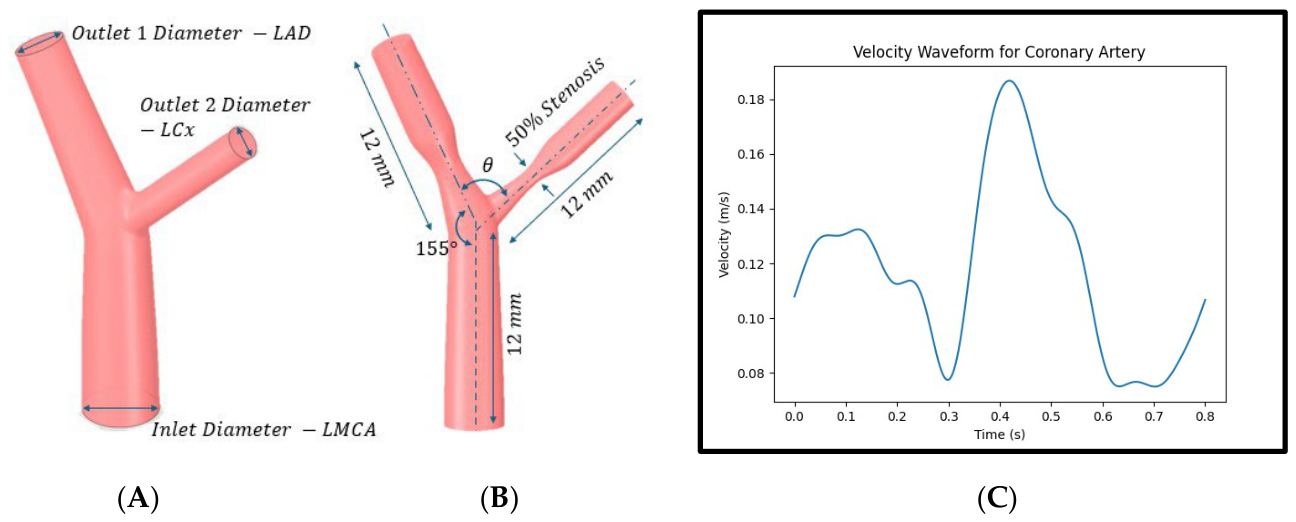
A bifurcated coronary artery geometry was approximated (Figure 1 and Figure 2) using an LMCA diameter of 4.86 ± 0.8 mm, LAD diameter of 3.4 ± 0.4 mm, and LCx diameter of 2.4 ± 0.45 mm [32,33,34]. The LMCA length was estimated as 9.1 ± 3.0 mm, whilst LAD and LCx lengths ranged between 50 and 150 mm. A bifurcation angle in the range of 53°–110° with a mean angle of 80° ± 10° (men) and 75° ± 10° (women) was used [35,36,37].
Atherosclerosis was mimicked by occluding the main vessel diameter, with a clinically significant 50% continuous stenosis used for both the LAD and LCx, post-bifurcation [38,39]. A stenosis equation (Equation (1)) [40] was been employed, where Dmin is the diameter at the stenosis point and Dhealthy is the diameter of the artery without stenosis.
S t e n o s i s   % = D h e a l t h y D m i n D h e a l t h y × 100
A custom Python script was used to automate the generation of the bifurcation models (Supplementary File S1). A dataset of 80 distinct geometries was generated and imported into SpaceClaim (ANSYS 2024R1, ANSYS Inc., Canonsburg, PA, USA). The full range of models generated is outlined in Table 1.

2.1.2. Boundary Conditions

Both steady-state and transient simulations were modelled. Under steady-state conditions, inlet velocity was fixed at 0.18 ms−1, representing peak velocity throughout the cardiac cycle [14]. Steady-state models focused on the maximum wall shear stresses (WSS) with the most developed flow patterns. The outlet condition was set to a systolic constant gauge pressure of 15,998.7 Pa or 120 mmHg [14,41]. Arteries were assumed to be rigid, with a no-slip boundary condition applied at the walls.
In transient simulations, a physiological artery waveform (Figure 2C) was processed using a fast Fourier transform to generate an equation to represent the cardiac cycle (Matlab 2024a, The MathWorks Inc., Natick, MA, USA). This equation was integrated into ANSYS via a user-defined function (Supplementary File S2) to define the inlet velocity at each time-step [19]. Transient simulations used a time-step of 0.001 s, with a maximum of 200 iterations per time-step over a total simulation time of 2.4 s (3 cardiac cycles for transient ‘independency’).

2.1.3. Material Properties

A multiphase Newtonian model was used to simulate blood as plasma and RBCs. The phases were set to be Newtonian, where viscosity is constant at 1.2 mPa·s for plasma and 6.31 mPa·s for the RBCs [14,19,42]. The Eulerian–Eulerian model with a laminar flow regime was used in ANSYS Fluent, and the volume fraction (VF) was set to 0.45, with the RBCs having a virtual mass coefficient of 0.5 and a diameter of 8 µm [43,44]. The plasma and RBC densities were 1003 kg·m−3 and 1096 kg·m−3, respectively. The RBC viscosity was calculated using Equation (2), where the whole blood viscosity was set as 3.5 mPa·s [45].
μ r b c = μ W h o l e b l o o d ( 1 V F r b c ) μ p l a s m a V F r b c

2.1.4. Meshing and Model Solution

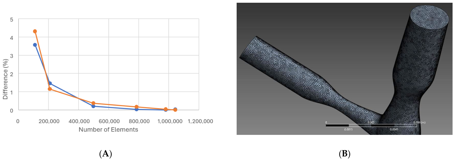
Mesh independency was established for a tetrahedral mesh by analysing flow variables for mean velocity and peak velocity in terms of their asymptotic behaviour with increased mesh size (Figure 3). The relative errors for the mesh size employed were below 5% as compared to the finest mesh evaluated. Further, meshing employed target values of maximum skewness <0.95 and an average skewness <0.3 with orthogonality ≥0.1, and an average aspect ratio <5 (Table 2). All simulations were solved using ANSYS Fluent (v24.1, ANSYS Inc., Canonsburg, PA, USA).
A semi-implicit method for pressure-linked equations was employed for the Eulerian–Eulerian mixture model. Equation (3) is the continuity equation and Equation (4) is the momentum equation, governing the flow for both phases, plasma (P) and RBC, where u is velocity (velocity components are given by u, v and w), p is pressure, ρ is density, α is VF, τ ̿ is the stress–strain tensor, KRBCP is the interface momentum exchange coefficient and Fext are the external forces.
t α R B C ρ R B C + · α R B C ρ R B C u R B C = 0
t α R B C ρ R B C + · α R B C ρ R B C u R B C = α R B C p + · τ ̿ R B C + R B C , P = 1 2 K R B C P u p u R B C + F e x t
All simulations were conducted on an Intel i7 13900K with 16 core processors and 32 GB DDR5 RAM. Wall-clock simulation times of both transient and steady-state simulations were recorded (Table 3). An outline of the model solver set-up is provided in Supplementary File S3.
The steady-state model was employed as the database for machine learning. For each simulation, 60 parameters were exported via a CSV file, including spatial coordinates, WSS per phase, as well as u and v per phase, and VF. CFD validation compared model predictions against existing literature. WSS was compared to CFD studies, whilst velocities were sourced from imaging studies.

2.2. Machine Learning

Table 4 outlines the ANNs trained, the number of geometries that were used for training them, and the number of previously unseen geometries that were used to test them.
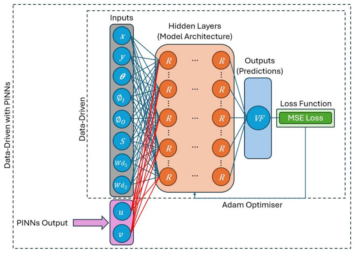
Two ANNs were examined to accurately predict haematocrit with limited data. The first was a standard data-driven ANN which predicted haematocrit and velocity components, serving as a control. The second used a PINN model to predict velocity components, which were fed back into the data-driven ANN (Figure 4). The PINN model was used to predict flow components as these were bounded by governing equations, whereas haematocrit does not explicitly have a governing equation and, hence, is not amenable to estimation using PINNs [46].
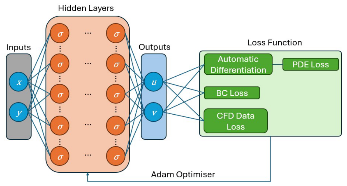
The PINN model used for this study (Figure 5) was based on two models and architectures from the literature [12,47]. In its original implementation it provided high accuracy for 2D predictions of velocity, but it has been modified to improve its time efficiency and compatibility with the training dataset. The modifications included the removal of the second-order differential terms from the loss function, and the use of one unique ANN to provide the u, v, and p predictions, instead of using three ANNs to predict them separately. This reduction in the number of ANNs used allowed for a reduction in computational overheads and hence solution times. Other modifications included removing the reliance on a VTK mesh and allowing nodes to be fed in from an Excel spreadsheet (CSV). Hyperparameters such as learning rate and patience were experimentally fine-tuned.

2.2.1. Pre-Processing Data and Training Data

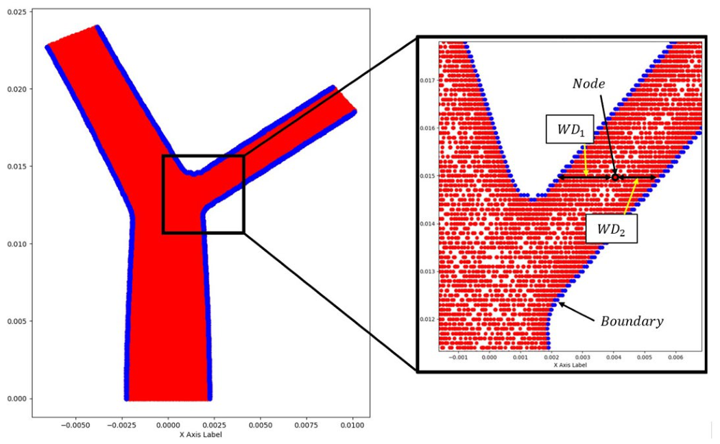
Predicting VF is a regression problem, where the outputs range in the interval [0, 1], indicating dominance of phase 2 (RBCs) or phase 1 (plasma). To account for model variation, wall distance was also used to inform the model about the positioning of the node relative to the geometry and boundary conditions. Two wall distances were provided to detect geometric constrictions such as stenosis (Figure 6).
Each 2D slice of the 3D geometry contained approximately 25,000 nodes, which were exported into a CSV file and extracted into the ANN models. All data was normalised using a scaling function (between minimum and maximum values) to a range between 0 and 1, for data driven models; this approach is purported to prevent overfitting and improve gradient stability [48].

2.2.2. Data-Driven ANN

A feedforward Multilayer Perceptron (MLP) dense ANN architecture was used for predicting VF (Figure 4). This architecture was selected for the data-driven ANN because of its universal approximator ability [49]. Preliminary tests found a configuration of 10 layers with 32 neurons each to yield the most repeatable predictions (Table 5).
Given the non-trivial depth of the architecture, a Rectified Linear Unit (ReLU) was applied to mitigate the vanishing gradient problem during back propagation [50]. The output was set to predict the VF at each node. The velocity components (u, v) were obtained via data-driven ANNs using a sparse and varied dataset.
The mean squared error (MSE) loss function was used in the training phase to estimate how well the predictions matched the ground truth from the CFD data. This measure is commonly used for regression tasks and is defined as follows:
M S E = 1 n i = 1 n y i y i ^ 2
where yi is the ground truth value, y i ^ is the ANN prediction, and n is number of data points predicted (Figure 6). To improve the generalisation ability of the ANN, drop-out layers and batch normalisation were used. Drop-out layers randomly deactivate neurons and force the network to undertake learning which is more robust and generalisable.

2.2.3. Physics-Informed Neural Network

The loss function for the PINN used was enforced using the governing equations for fluid flow. The continuity component of the Navier–Stokes equation was added as a term to the loss function of Equation (6), a standard approach to using PINNs. The Navier–Stokes equations did not include the time (t) and gravity (gx) terms or the third spatial component (w) as the term for the loss function uses a two-dimensional equation set. A ROM was used which excluded the second-order differential terms (Equation (6)), as it predicts u and v more efficiently; the approach used followed the methodology presented by Fox et al. [24].
L o s s P 1 = i = 1 m u i x + v i y
L o s s P 2 = i = 1 m u i u i x + v i u i y + 1 ρ p i x
L o s s P 3 = i = 1 m u i v i x + v i v i y + 1 ρ p i y
L o s s B o u n d a r y = i = 1 m u l u b o u n d a r y , i 2
L o s s C F D D a t a = 1 n i = 1 n u l u C F D , i 2  
where u and v represent velocity components in the x and y directions respectively, p represents pressure, and µ represents dynamic viscosity. Equation (6) represents a loss term for the conservation of mass for incompressible flow, i.e., the continuity equation. The x and y components for the conservation of momentum are simplified into Equations (7) and (8), i.e., a loss term for the Euler momentum for fluid flow along x- and y-axes, respectively. Hence, these are the terms used to estimate the loss function in the physics-informed equations. These loss terms are used to determine the error when using the ANN to predict values for the variables u, v, and p. In brief, Equations (6)–(8) describe the partial differential equation (PDE) loss. Equation (9), instead, is used to enforce the boundary conditions by measuring the error on the predicted boundary velocity values. Equation (10) has the form of Equation (5), but is specific to the velocity vector; here, it defines the error on the sparse data points that are fed into the PINN model to guide it to a solution during the training stage of the ANN. An assumption of this approach is that inlet conditions may not be fully defined, or known [12]. Note that the data loss is calculated on the input–output sparse data pairs, whilst the physics-informed losses are calculated using user-specified samples from across the entire input domain. The total loss is then
L o s s t o t a l = L o s s P 1 + L o s s P 2 + L o s s P 3 + L o s s B o u n d a r y + L o s s C F D D a t a
The ANN learning algorithm will drive all the components in Equation (11) to zero, forcing the PINN to comply with both the CFD data and the physics-informed knowledge. The components of the loss function have been given equal weight in this study, as shown in Equation (11), which combines all the loss function terms from Equations (6)–(10). This strategy applies an equal importance in the training of the PINN across the data loss, the continuity equation, the Euler equations, and, critically, the loss term at the boundary. The latter would otherwise be underweighted given that there is a class imbalance as measured by the volume of fluid at the boundary and otherwise. Hence, this approach avoids underestimating a disproportionate error at the boundary, and thereby allows for the formation of a boundary layer appropriate for the fluid’s viscosity being approximated.
A sigmoid activation function was used for its well-defined bounds between 0 and 1 which is ideal for predicting the u and v values correctly, especially near the wall where near-zero values might elude convergence. This function ‘squashes’ extreme, small or large, values towards the values of 0 and 1, respectively. In brief, this sigmoid activation function is applied to all layers of the PINN, and serves as an alternative to the ReLU activation commonly used in MLPs; however, unlike ReLU, whose second derivative is zero almost everywhere, the sigmoid activation function is smooth and retains non-zero higher-order derivatives, enabling the sigmoid function to better approximate PDEs. The PINN set-up is summarised in Table 6.

2.2.4. PINN into Data-Driven ANN

Predictions made by the PINN model for u and v (Table 6) for the test geometry were fed into a data-driven ANN (Table 5) to make predictions on VF (Figure 4). This aids the data-driven ANN to make more accurate VF predictions. This is because velocity components have correlations with VF that are not explicitly defined but can be captured by the ANN to improve predictions.

3. Results

3.1. CFD Validation

Table 7 compares CFD data with the highest geometric variability, encompassing varying bifurcation angles. This data was cross-referenced with eight studies to validate key parameters such as mean and maximum WSS and velocity in both normal and stenosed arteries [51,52,53,54,55,56,57,58].
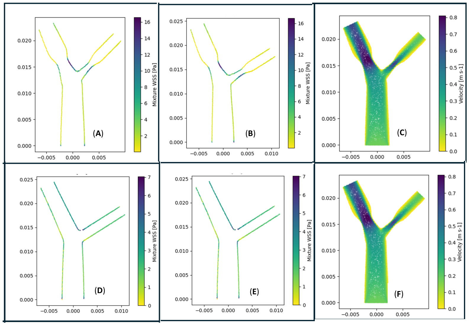
For normal arteries, the mean velocity of the generated data ranged from 0.217 to 0.220 ms−1, aligning with Doppler measurements (0.15–0.49 ms−1). The maximum velocity predicted (~0.5 ms−1) was within the range reported in the literature, ranging from 0.43 ms−1 [51] up to 0.89 ms−1 [52]. In stenosed arteries, both mean and peak velocities increased, nearly doubling for peak velocity. The mean velocity increased by approximately 15%, compared to a 22% increase reported in the literature [51]. The maximum velocity (~0.8 ms−1) predicted was to within 11% of Doppler measurements available in the literature [51].
The maximum WSS predicted for stenosed arteries (16.7 Pa) also fell within the range of these studies from the literature (5.2–42 Pa) [54,55,56,57]. Normal arteries exhibited maximum WSS values exceeding 7 Pa, consistent with the generated data. The mean WSS for normal arteries was 1.9 Pa, showing a 17% increase from normal to stenosed conditions. Overall, CFD studies indicated a 28% increase in mean WSS between stenosed and normal arteries.
Regions of high WSS (12–16 Pa) were located at the stenosis ‘throat’ and low WSS regions (<1 Pa) immediately after (Figure 7). Peak WSS (7–8 Pa) at the split of bifurcation was predicted to be 7–8 Pa, with a reduced WSS after the artery begins to split (<1 Pa; Figure 7). In a stenosed model, maximum velocity (0.8 ms−1) was measured at the stenosis, dropping to zero near the wall after, with lower peak velocity predicted for the healthy artery (0.5 ms−1).

3.2. ANN Flow Predictions

The ANN results are presented for a select few models consisting of the ‘worst’ and ‘best’ predictions for the data-driven approach, and data-driven and PINN approach. Forty data-driven ANN predictions were made, to give a broad range of results, and initially intended to identify some with ‘greater’ accuracy. However, it was only necessary to solve 20 data-driven and PINN models as even for extreme cases, model predictions of flow outputs were to within 8.5% of CFD predictions. VF is the key output prediction for two-phase flow presented. Both the average percentage error (APE; Equation (12)) and MSE (Equation (5)) have been evaluated.
A P E = 1 n i = 1 n y i y i ^ y i × 100
PINNs are useful for resolving problems with unknown geometry as they do not rely on data to resolve a problem, instead relying on a custom loss function which for fluid flow analysis can be designed to satisfy the Navier strokes equation [12,47], therefore mimicking a CFD solver. Five PINN ‘only’ models were initially solved and evaluated, to validate the flow output velocity (u, v), used for the data-driven and PINN model, against CFD predictions ahead of its implementation into a data-driven ANN.

3.2.1. Data-Driven ANN

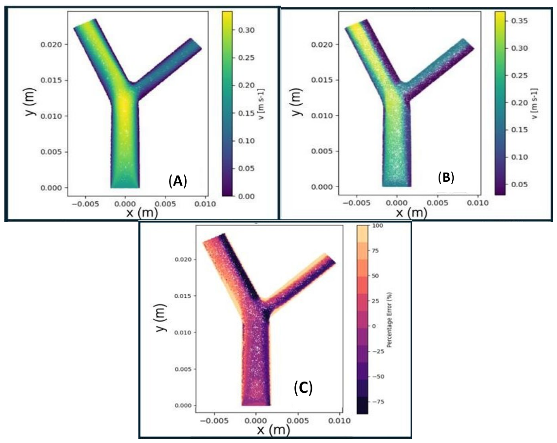
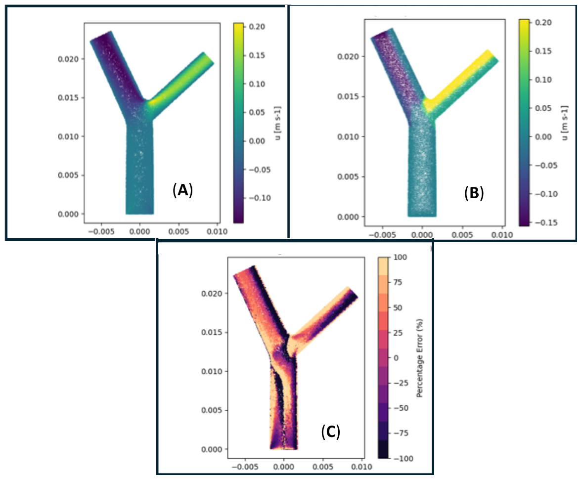
Data-driven ANN predictions of flow included transverse flow predictions with errors ranging from 51% to 72% for ‘best’ and ‘worst’ models (Table 8), respectively, amongst the 40 models solved. Data-driven predictions for u velocity exhibited a clear shift in flow (Figure 8). This can be observed at the centre of the left main coronary artery (i.e., the ‘parent’ artery); the peak velocity approximately at the central radial position of the left circumflex artery shifts towards the wall of this artery in the data-driven ANN model. There was also difficulty in predicting the flow at the boundary of walls, with the velocity for u at the wall not approaching zero (Figure 8), noticeable in both branching arteries, where errors remain high.
Data-driven ANN predictions of streamwise flow included APEs ranging from 35% to 47% for ‘best’ and ‘worst’ models, respectively (Table 8). Streamwise flow predictions were better than predictions for transverse flow, with peak flow predicted through the centre of the left main coronary artery and left anterior descending coronary artery (Figure 9). However, the velocity for v still had noticeable errors when predicting flow at the wall of arteries, which can be observed in particular for the left circumflex artery.
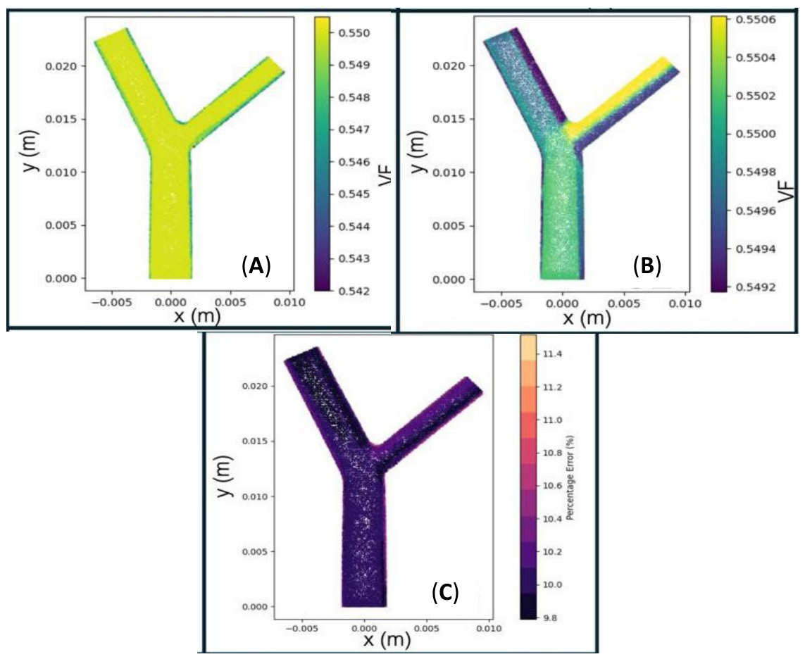
The data-driven ANN predictions of VF included APEs not exceeding 15% (Table 8), with predictions ranging from 12 to 15% across the 40 models solved. This range of %-error was lower than the %-error when predicting u and v, but it appears to be due to a combination of two different errors. Firstly, the difference in the absolute value predicted was lower than for CFD models (Figure 10). Secondly, the VF distribution did not match the CFD prediction along wall boundaries (Figure 10), which are regions where predictions of velocity (u, v) are poor.
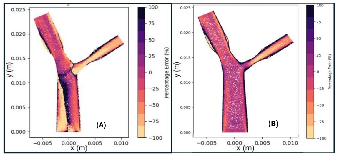
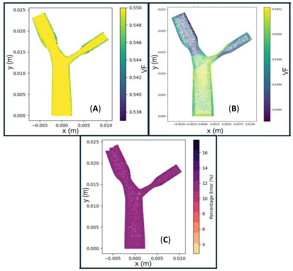
For models where stenosis was included, the data-driven ANN predictions for the stenosed models broadly matched the trends observed for otherwise ‘healthy’ bifurcation models. There were difficulties in predicting central flow through the left circumflex and left descending arteries, and peak %-errors occurring at the walls of the left circumflex coronary artery for u and v (Figure 11). There was also flow separation through the centre of the flow of the left main coronary artery. Predictions of VF remained within a range of 12–15% error as compared to the CFD model (Figure 12).

3.2.2. Physics-Informed Neural Network and Data-Driven ANN

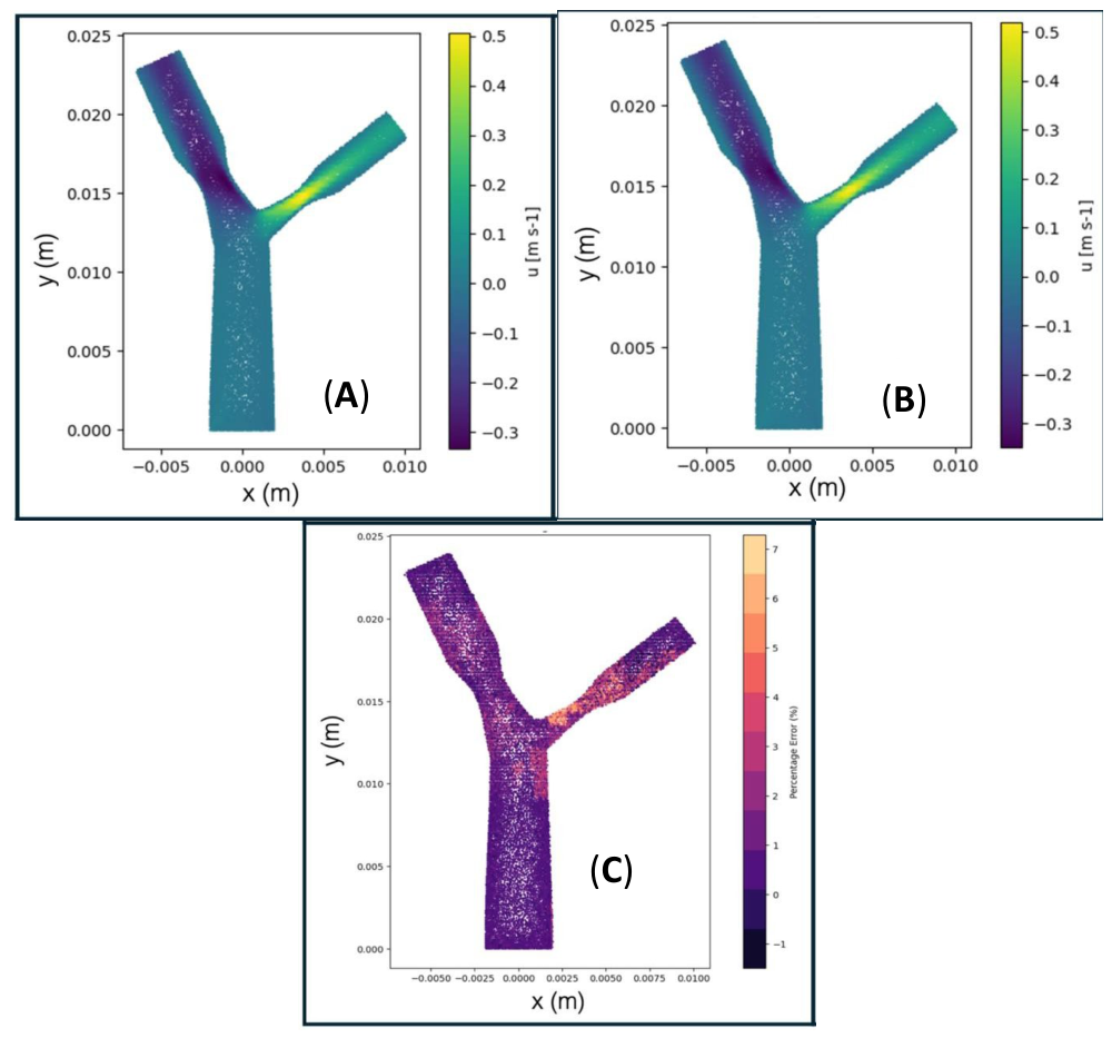
Five coronary artery bifurcation geometries, with stenosis, were evaluated using a PINN model. Predictions for u and v across these models led to errors ranging between 6 and 8.5% across the five models (Table 9). For transverse flow, the highest error was located at the stenosis ‘throat’ of the left circumflex artery, where flow patterns transition from the left main descending artery to the bifurcation and then undergo a venturi effect within the narrower left circumflex artery (Figure 13). The patterns of flow matched those from the CFD simulations, with peak values for u of around 0.5 m/s.
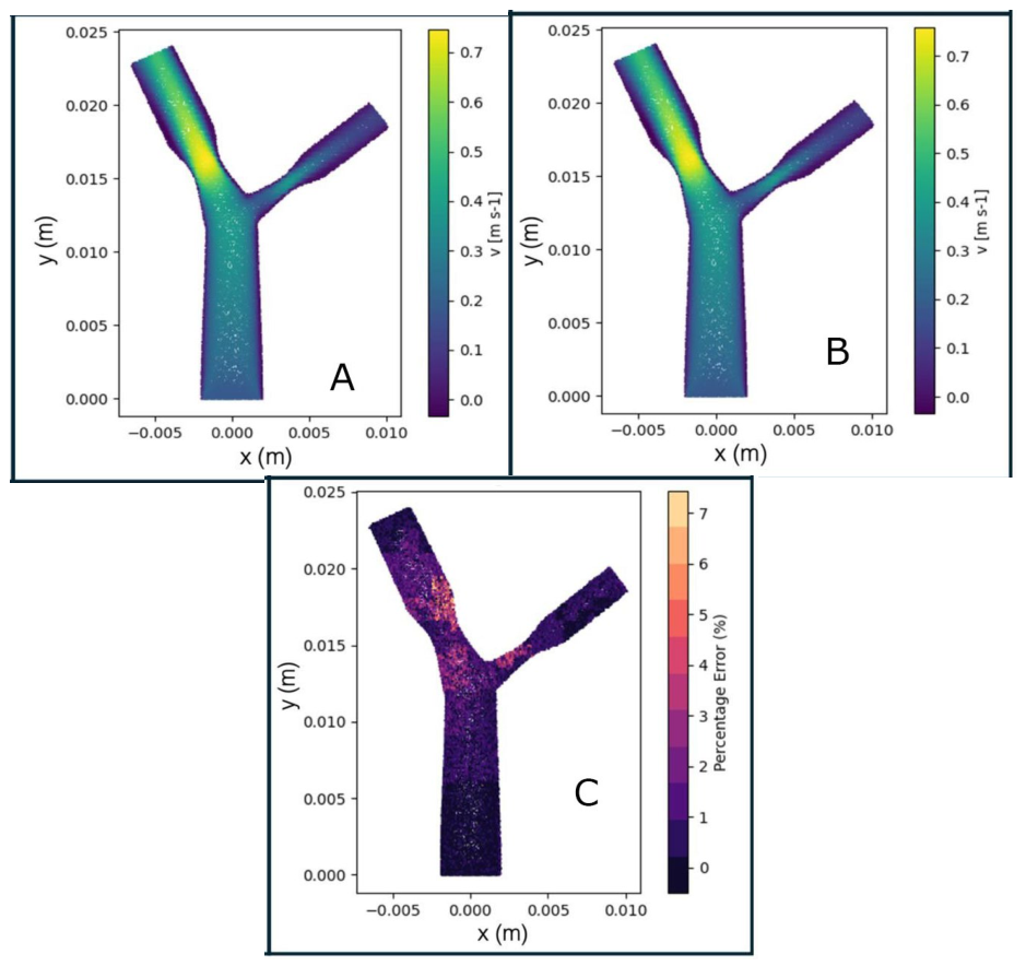
Streamwise flow patterns predicted using the PINN model were representative of the CFD results. Peak values for v were around 0.7 m/s for both the CFD and PINN models (Figure 14). Regions with highest errors were around the stenosis regions of both left circumflex and left anterior descending arteries (Figure 14), consistent with regions of highest error for transverse flow. Errors for streamwise flow were lower than for transverse flow, with APE for v ranging from 5.63 to 6.98% (Table 9) across the five models solved purely using a PINN.
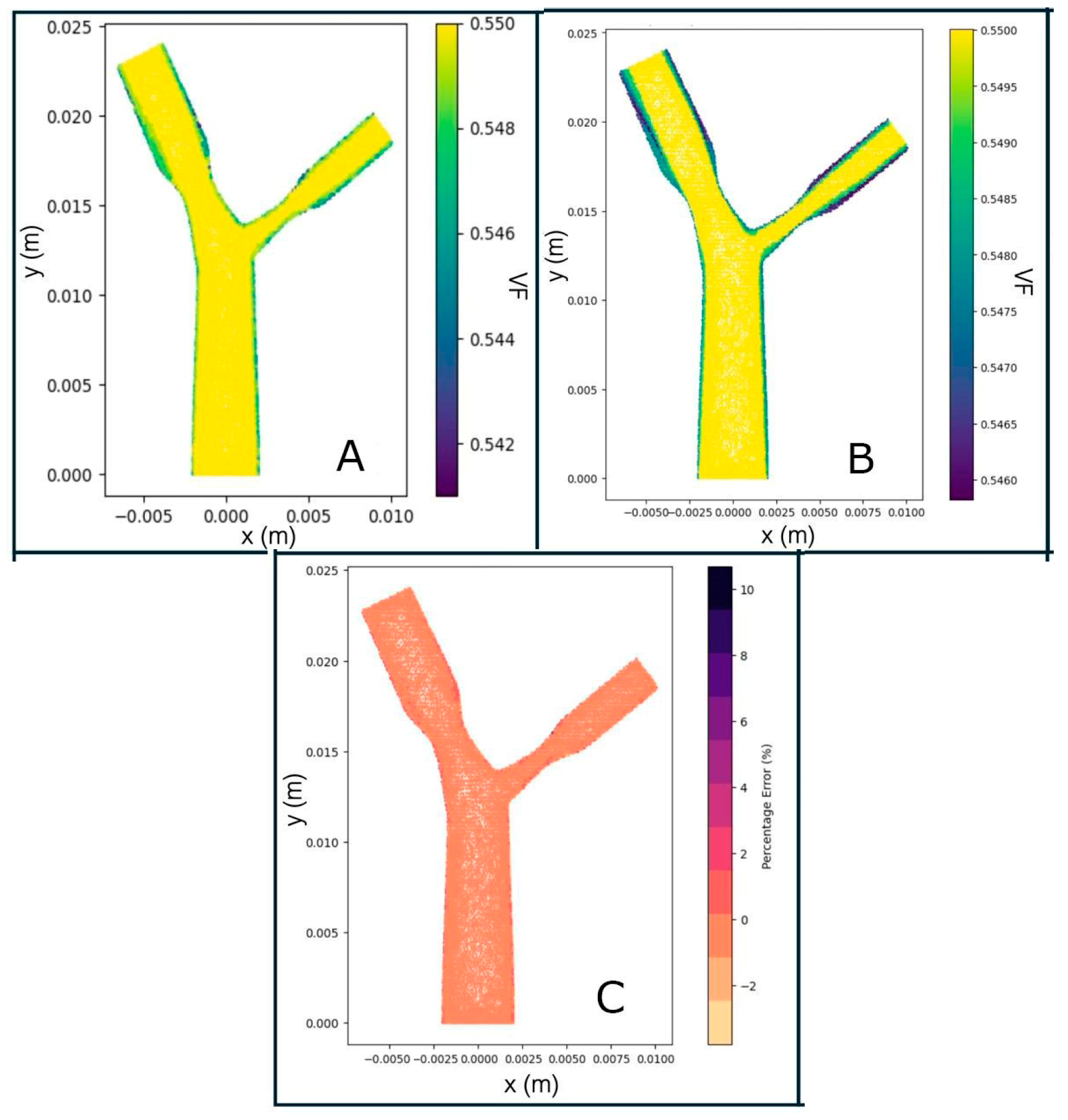
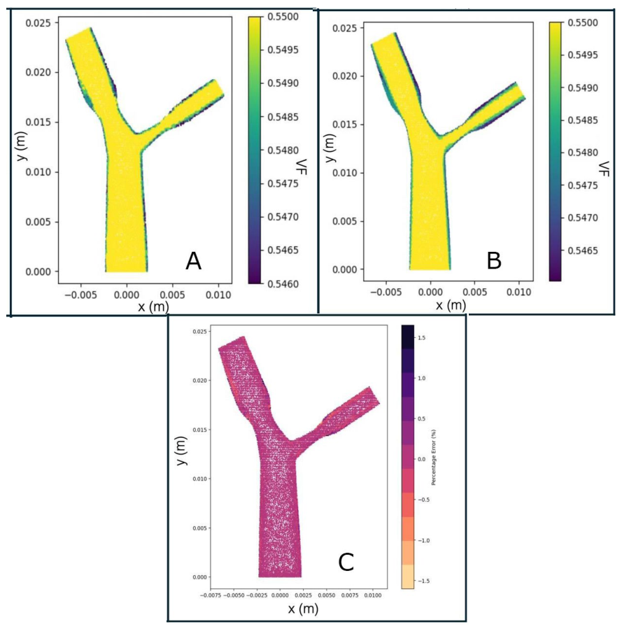
Using the PINN outputs for u and v as an input into a data-driven ANN led to excellent predictions for VF by the data-driven ANN across the 20 models solved. The APE for VF ranged from 0.04% to 0.05%, for ‘best’ and ‘worst’ predictions, respectively (Table 10). Predictions for VF, using the PINN–data-driven ANN combination, closely matched the CFD predictions for stenosed arteries including VF distribution through flow toward the centre of the arteries and at the walls of the arteries (Figure 15 and Figure 16).

3.3. Solution Times

On average, data-driven ANN models took less than an hour to solve (0.78 h; Table 11).
The use of PINNs led to solution times, on average, of 4.4 h (PINN) and 4.9 h (PINN + data-driven ANN). These solution times compare to a CFD steady-state solution time of 0.8 h. However, steady-state models for blood flow do not predict peak flow conditions; this requires a transient CFD simulation. For comparison, transient CFD runs took 90× longer than steady-state CFD simulations, and 14× longer than a hybrid data-driven ANN + PINN model (Table 11).

4. Discussion

The major finding of this study is the ability to leverage PINNs on a multiphase problem to provide highly accurate results for VF, to within <<1% of CFD predictions. The ROM-PINN model achieves velocity predictions which are in the range of 5–8.5% of CFD predictions, noting that the CFD results for the 80 models used to train the ANNs, including healthy and stenosed arteries, fell in the expected range from the literature [53,54,56,57] including clinical studies [51,52,58]. This level of accuracy in PINNs, when used as an input for u and v velocity components into a data-driven ANN, is key in enabling the highly accurate prediction of the two phases of flow of blood within a left coronary artery model.
Pure data-driven models face challenges in velocity predictions due to only using geometric inputs and data scarcity; although this only results in errors for predicting VF in the 12–15% range, the profile of haematocrit distribution is poor, particularly around the boundaries of artery walls. Indeed, twice as many purely data-driven models were solved than those incorporating PINNs. This approach was necessary to identify some better performing models. However, using PINNs as an input for u and v into a data-driven model led to predictions of VF which better approximated CFD predictions by orders of magnitude.
The hybrid PINN and data-driven model used in this study accurately predicts haematocrit by leveraging the inherent link between haematocrit and velocity. Despite this being an undefined relationship, the model identifies regions of reduced velocity corresponding to higher haematocrit levels. This ability of the ANN suggests the potential for rapid identification in patient-specific geometries.
Despite longer simulation times compared to steady-state runs, the hybrid model outperforms transient CFD runs in terms of time by a factor of 14×. The use of a ROM-PINN, in particular, enables an improvement in solution time compared to CFD solutions. The use of a ROM-PINN approach has been found to be able to lead to high-accuracy predictions, while being highly efficient in terms of solution times when compared to fully solving all equations of flow [24]. It is noted that a ROM-PINN and data-driven approach can be directly trained on key results for transient flow, whereas a CFD model needs to fully solve such transient simulations.
Data-driven ANNs typically demand a substantial dataset to mitigate overfitting and to aid generalisation. To provide a sufficiently varied dataset, which is necessary when trying to quantify and predict patient-specific geometry, a very large dataset would be required. This was a key finding when initially running the MLP ANN. Initially, overfitting posed a significant challenge, leading to predictions often deviating drastically from scale and failing to capture flow patterns accurately. This was probably due to the very large number of parameters (deep ANN weights) that had to be fitted to the data. Therefore, techniques such as drop-out layers and batch normalisation were employed.
Whilst general flow patterns were predicted, their relative positioning within a tested geometry could become skewed (e.g., Figure 8 and Figure 15). For instance, the exaggeration of the zero-velocity wall boundary condition is pronounced at the bottom of the right artery, whilst virtually absent at the top boundary (e.g., Figure 9). One reason for this discrepancy lies in how wall distance is calculated. Wall distance is determined not by the normal distance from the wall, but by the closest boundary point on the same x-axis (Figure 6). This oversight becomes apparent when the bifurcation angles increase, as it causes wall distances to shift in the x-direction, despite their relative positions remaining the same. Consequently, the ANN model encounters learning difficulties, leading to shifts in flow patterns. Predictions in the streamwise direction exhibit higher accuracy, with an APE across the whole domain of 47–72% in the transverse direction. For example, flow patterns are correctly represented but on an incorrect scale (Figure 11).
There was some difficulty by the MLP ANN to predict VF with the correct scale, despite the measures taken to improve model generalisation. As a result, more inputs, other than just the geometrical data, were required to be fed into the data-driven model. However, in a clinical setting some of the addition data necessary for the MLP ANN, for an unseen geometry, may not be available. Instead, the ROM-PINN approach enabled flow predictions of greater accuracy, in essence for unseen geometries.
The intention of this study was not to directly compare a data-driven approach to a PINN approach for modelling VF. The initial intention was to identify the benefits, limitations and applications of each independently. However, the MSE for VF is four orders of magnitude lower when a ROM-PINN approach is used to produce a u and v input into a data-driven model than when using a data-driven approach alone. The best-performing models have an APE for VF of 12% for data-driven models, as compared to 0.04% when a ROM-PINN was used. The results from this hybrid ROM-PINN and data-driven approach, with errors of <<1% for VF, and in the range of 5–8.5% for velocity components, are comparable to a PINN model employed for two-phase flow as applied to thermal systems where errors were estimated to be below 2.8% [31].

Limitations

As with any study, there are limitations. This study has focused on the use of neural networks to predict two-phase flows and has explored methods by which to do so efficiently. The CFD results provide the direct baseline for comparison of neural network predictions, and form the training and testing data for data-driven machine learning. However, validation of the CFD data itself is in the form of comparison to ranges in the literature. The 80 distinct geometries and CFD simulations generated for training and the 40 distinct CFD models employed for testing have not been individually validated against physical measurements. However, we have identified that if a patient-specific ROM-PINN were to be pursued, data would likely need to be obtained from more than 80 patients. This is because of the more complicated anatomy, and greater variability in flow patterns. Therefore, it would be useful to explore whether applying a different weighting to the terms of the loss function or a Proper Orthogonal Decomposition (POD) approach to ROM when generating the equation sets employed in PINNs would enhance efficiency of models. Given the proof-of-concept nature of the work presented, and the high accuracy of the model, further optimisation of the weight of each of the terms of the loss function has not been explored. However, a sensitivity study might increase the accuracy and generalisation ability of the model. Regardless, this study has demonstrated that the flow of a two-phase fluid can be predicted via machine learning, where data-driven learning is constrained using simplified equation sets.
The CFD dataset used for data training used a multiphase Newtonian–Newtonian assumption. The architecture used for data-driven machine learning is preferable for Newtonian models [59]. However, in diseased states, the use of a limited non-Newtonian model may have implications for disease progression; for example, regions of low wall shear stress in aneurysms have an increased risk of rupturing. As blood is a shear-thinning fluid [18], it is these regions experiencing low shear which are most sensitive to non-Newtonian effects when calculating wall shear stress [60]. Hence, developing ANNs for clinical applications, such as links between haemodynamic parameters [61], WSS [62] and atherosclerosis, may require further extension into non-Newtonian multiphase models [63]. Regardless, this study demonstrates that a hybrid data-science and ROM-PINN model can be used to machine learn the flow of the two main phases of blood. However, this study refrains from making predictions of the risk for thrombosis formation. While CFD models that make such predictions exist, they employ non-Newtonian formulations to predict the RBC phase, and they employ parameters such as residence time for platelets [19]. In 2021, Owen et al. [19] used a multiphase non-Newtonian model to examine 50% stenosis. Their findings revealed areas of low WSS (<1 Pa) downstream of the stenosis. Conversely, in healthy arteries, WSS typically ranged between 1 and 7.5 Pa. These values align well with the predictions of the CFD models and the data-driven ROM-PINN model. The predictions of WSS in these CFD studies have the limitation of assuming a rigid vessel wall, whereas coronary arteries are known to be viscoelastic [64]. While the impact on flow predictions may be limited, this may alter predictions of stress. The extension of the work presented in this study to include wall vessel mechanics would require a fluid–structure interaction [65,66] approach to modelling, where structural deformation is directly coupled to localised wall velocity and full stress tensor is used to calculate the wall deformation either simultaneously [67] or iteratively [68]. Two-phase flow is compatible with fluid–structure interaction modelling [69].
The flow regime for this study has used a laminar assumption. In diseased coronary arteries, turbulent flow might be expected. This might be mitigated by the assumption of the wall of the artery to be rigid, which in some studies has been found to limit factors such as distortion of the artery that could contribute to turbulence [70]. For application to a patient-specific model, turbulence may need to be considered in the simulation pipeline. The ROM approach to flow modelling via neural networks has previous been evaluated for turbulent flows [24,71], and as such may be compatible with a turbulence model. Regardless, our findings are consistent with studies in the literature [15,19,72,73]. While there are limitations to using a laminar flow regime for CFD modelling of flow through arteries, the results are self-consistent. For patient-specific simulations, there are examples in the literature where turbulence models have been found to produce counter-intuitive results, such as a reduction in WSS for a diseased state as compared to a healthy model, where increased WSS might be expected [74]. Machine learning of turbulent flow, implications for the boundary layer and its implementation as a loss function merit further study.

5. Conclusions

Combining an MLP ANN and a PINN yields multiphase flow predictions for the two main phases of blood, to within 8.5% for velocity components and <<1% for volume fraction as compared to CFD simulations. This hybrid model runs 14 times faster than equivalent transient CFD simulations, and to time-scales comparable to steady-state simulations.

Supplementary Materials

The following supporting information can be downloaded at: https://www.mdpi.com/article/10.3390/fluids11050118/s1, Supplementary File S1: Code for Generating Varying Geometries. Supplementary File S2: UDF Code for Transient Simulations. Supplementary File S3: CFD Solver Setup Parameters.

Author Contributions

J.C.: conceptualisation, analysis, writing—original draft and editing. B.S.: conceptualisation, data curation, formal analysis, methodology, software, investigation, validation, writing—original draft and editing. W.F.: analysis, writing—review and editing. M.C.: conceptualisation, analysis, methodology, writing—review and editing. D.M.E.: conceptualisation, analysis, supervision, project administration, methodology, writing—review and editing. All authors have read and agreed to the published version of the manuscript.

Funding

J.C. was supported by the Engineering and Physical Sciences Research Council [grant number: EP/W524396/1].

Institutional Review Board Statement

Not applicable.

Informed Consent Statement

Not applicable.

Data Availability Statement

Relevant data are available upon reasonable request.

Conflicts of Interest

The authors declare no conflicts of interest.

Abbreviations

APEAverage Percentage Error
CFDComputational Fluid Dynamics
CSVComma-Separated Variable
LADLeft Anterior Descending
LCxLeft Circumflex
LMCALeft Main Coronary Artery
MLPMultilayer Perceptron
MRIMagnetic Resonance Imaging
MSEMean Squared Error
nNumber of Nodes
NNNeural Network
PDEPartial Differential Equation
PINNPhysics-Informed Neural Network
RBCRed Blood Cell
ROMReduced Order Model
uVelocity in x Direction
vVelocity in y Direction
VFVolume Fraction
wVelocity in z Direction
WSSWall Shear Stress
DhealthyDiameter of Non-Stenosed Artery
DminDiameter at Stenosis Point
KRBCPInterface Momentum Exchange Coefficient
VFRBCRed Blood Cell Volume Fraction
VF Volume Fraction
pPressure
yiGround Truth Value
y i ^ Predicted Value
FextExternal Forces
uVelocity
μplasmaPlasma Viscosity
μrbcRed Blood Cell Viscosity
μwholebloodWhole Blood Viscosity
τ̿ Stress–Strain Tensor

References

  1. Wentzel, J.J.; Chatzizisis, Y.S.; Gijsen, F.J.H.; Giannoglou, G.D.; Feldman, C.L.; Stone, P.H. Endothelial shear stress in the evolution of coronary atherosclerotic plaque and vascular remodelling: Current understanding and remaining questions. Cardiovasc. Res. 2012, 96, 234–243. [Google Scholar] [CrossRef]
  2. Lewington, W.; Herrington, B.; Lacey, P.; Sherliker Armitage, J.; Lewington, S. Epidemiology of atherosclerosis and the potential to reduce the global burden of atherothrombotic disease. Circ. Res. 2016, 118, 535–546. [Google Scholar] [CrossRef] [PubMed]
  3. Malek, A.M.; Alper, S.L. Hemodynamic shear stress and its role in atherosclerosis. JAMA 1999, 282, 2035. [Google Scholar] [CrossRef] [PubMed]
  4. Fuster, E.F.; Prediman, S.; Valentin, K. Coronary plaque disruption. Circulation 1995, 92, 657–671. [Google Scholar] [CrossRef] [PubMed]
  5. Louvard, Y.; Thomas, M.; Dzavik, V.; Hildick-Smith, D.; Galassi, A.R.; Pan, M.; Burzotta, F.; Zelizko, M.; Dudek, D.; Ludman, P.; et al. Classification of coronary artery bifurcation lesions and treatments: Time for a consensus! Catheter. Cardiovasc. Interv. 2008, 71, 175–183. [Google Scholar] [CrossRef]
  6. Chatzizisis, Y.S.; Coskun, A.U.; Jonas, M.; Edelman, E.R.; Feldman, C.L.; Stone, P.H. Role of endothelial shear stress in the natural history of coronary atherosclerosis and vascular remodeling. molecular, cellular, and vascular behavior. J. Am. Coll. Cardiol. 2007, 49, 2379–2393. [Google Scholar]
  7. Schroder, J.; Prescott, E. Doppler echocardiography assessment of coronary microvascular function in patients with angina and no obstructive coronary artery disease. Front. Cardiovasc. Med. 2021, 29, 723542. [Google Scholar] [CrossRef]
  8. Tests and Treatments: MRI Scan. NHS Inform. 10 November 2023. Available online: https://www.nhsinform.scot/tests-and-treatments/scans-and-x-rays/mri-scan/#whathappens-during-an-mri-scan (accessed on 10 May 2026).
  9. Zhang, X.; Mao, B.; Che, Y.; Kang, J.; Luo, M.; Qiao, A.; Liu, Y.; Anzai, H.; Ohta, M.; Guo, Y.; et al. GaoyangL Physics-informed neural networks (PINNs) for 4D hemodynamics prediction: An investigation of optimal framework based on vascular morphology. Comput. Biol. Med. 2023, 164, 107287. [Google Scholar] [CrossRef] [PubMed]
  10. Pour-Ghaz, I.; Manolukas, T.; Foray, N.; Rawal, J.R.A.; Ibebuogu, U.N.; Khouzam, R.N. Accuracy of non-invasive and minimally invasive hemodynamic monitoring: Where do we stand? Ann. Trans. Med. 2019, 7, 421. [Google Scholar] [CrossRef]
  11. Brunette, J.; Mongrain, R.; Laurier, J.; Galaz, R.; Tardif, J.C. 3D flow study in a mildly stenotic coronary artery phantom using a whole volume PIV method. Med. Eng. Phys. 2008, 30, 1193–1200. [Google Scholar] [CrossRef]
  12. Arzani, A.; Gambaruto, M.; Chen, G.; Shadden, S.C. Lagrangian wall shear stress structures and near-wall transport in high-Schmidt-number aneurysmal flows. J. Fluid. Mech. 2016, 790, 158–172. [Google Scholar]
  13. Gallo, D.; Santis, G.; Negri, F.; Tresoldi, D.; Ponzini, R.; Massai, D.; Deriu, M.; Segers, P.; Verhegghe, B.; Rizzo, G.; et al. On the use of in vivo measured flow rates as boundary conditions for image-based hemodynamic models of the human aorta: Implications for indicators of abnormal flow. Ann. Biomed. Eng. 2012, 40, 729–741. [Google Scholar]
  14. Owen, D.G.; Schenkel, T.; Shepherd, D.E.T.; Espino, D.M. Assessment of surface roughness and blood rheology on local coronary haemodynamics: A multi-scale computational fluid dynamics study. J. R. Soc. Interface 2020, 17, 20200327. [Google Scholar] [CrossRef]
  15. Picart, C.; Piau, J.M.; Galliard, H. Human blood shear yield stress and its hematocrit dependence. J. Rheol. 1998, 42, 1–12. [Google Scholar] [CrossRef]
  16. Red Cross Blood. Haematocrit. 2023. Available online: https://www.redcrossblood.org/donate-blood/dlp/hematocrit.html (accessed on 10 May 2026).
  17. Wells, R.; Merrill, E. Influence of flow properties of blood upon viscosity-hematocrit relationships. J. Clin. Investig. 1962, 41, 1591–1598. [Google Scholar] [CrossRef]
  18. Chatpun, S.; Cabrales, P. Effects of plasma viscosity modulation on cardiac function during moderate hemodilution. Asian J. Trans. Sci. 2010, 4, 102–108. [Google Scholar] [CrossRef]
  19. Owen, D.G.; de Oliveira, D.C.; Neale, E.K.; Shepherd, D.E.T.; Espino, D.M. Numerical modelling of blood rheology and platelet activation through a stenosed left coronary artery bifurcation. PLoS ONE 2021, 16, E0259196. [Google Scholar]
  20. Walton, B.L.; Lehmann, M.; Skorczewski, T.; Holle, L.A.; Beckman, J.D.; Cribb, J.A.; Mooberry, M.J.; Wufsus, A.R.; Cooley, B.C. Elevated hematocrit enhances platelet accumulation following vascular injury. Blood 2017, 129, 2537–2546. [Google Scholar] [CrossRef] [PubMed]
  21. Jin, Y.Z.; Zheng, D.H.; Duan, Z.Y.; Lin, Y.Z.; Zhang, X.Y.; Wang, J.R.; Han, S.; Wang, G.F.; Zhang, Y. Relationship between hematocrit level and cardiovascular risk factors in a community-based population. J. Clin. Lab. Anal. 2015, 29, 289293. [Google Scholar] [CrossRef]
  22. Gotoh, S.; Hata, J.; Ninomiya, T.; Hirakawa, Y.; Nagata, M.; Mukai, N.; Fukuhara, M.; Ikeda, F.; Ago, T.; Kitazono, T.; et al. Hematocrit and the risk of cardiovascular disease in a Japanese community: The Hisayama Study. Atherosclerosis 2015, 242, 199–204. [Google Scholar] [CrossRef]
  23. Vinuesa, R.; Brunton, S. Enhancing computational fluid dynamics with machine learning. Nat. Comput. Sci. 2022, 2, 358–366. [Google Scholar] [CrossRef]
  24. Fox, W.; Sharma, B.; Chen, J.; Castellani, M.; Espino, D.M. Optimising physics-informed neural network solvers for turbulence modelling: A study on solver constraints against a data-driven approach. Fluids 2024, 9, 279. [Google Scholar] [CrossRef]
  25. Maziar, R.; Alireza, Y.; George, E.K. Hidden fluid mechanics: A Navier-Stokes informed deep learning framework for assimilating flow visualization data. arXiv 2018, arXiv:1808.04327. [Google Scholar] [CrossRef]
  26. Cai, S.; Mao, Z.; Wang, Z.; Yin, M.; Karniadakis, G.E. Physics-informed neural networks (PINNs) for fluid mechanics: A review. Acta Mech. Sin. 2021, 37, 1727–1738. [Google Scholar] [CrossRef]
  27. Pioch, F.; Harmening, J.; Muller, A.; Peitzmann, F.; Schramm, D.; el Moctar, O. Turbulence modeling for physics-informed neural networks: Comparison of different RANS models for the backward-facing step flow. Fluids 2023, 8, 43. [Google Scholar]
  28. Bukac, M.; Manojlović, I.; Muha, B.; Vlah, D. Reduced Order Modeling of Partial Differential Equations on Parameter-Dependent Domains Using Deep Neural Networks. Available online: https://ssrn.com/abstract=5762809 (accessed on 10 May 2026).
  29. Brunton, S.L.; Proctor, J.L.; Kutz, J.N. Discovering governing equations from data by sparse identification of nonlinear dynamical systems. Proc. Natl. Acad. Sci. USA 2016, 113, 3932–3937. [Google Scholar] [CrossRef] [PubMed]
  30. Fu, J.; Xiao, D.; Fu, R.; Li, C.; Zhu, C.; Arcucci, R.; Navon, I.M. Physics-data combined machine learning for parametric reduced-order modelling of nonlinear dynamical systems in small-data regimes. Comput. Method. Appl. Mech. Eng. 2023, 404, 115771. [Google Scholar] [CrossRef]
  31. Jalili, D.; Jang, S.; Jadidi, M.; Giustini, G.; Keshmiri, A.; Mahmoudi, Y. Physics-informed neural networks for heat transfer prediction in two-phase flows. Int. J. Heat. Mass. Trans. 2024, 221, 125089. [Google Scholar] [CrossRef]
  32. Reig, J.; Petit, M. Main trunk of the left coronary artery: Anatomic study of the parameters of clinical interest. Clin. Anat. 2004, 17, 6–13. [Google Scholar] [CrossRef]
  33. Paul, A.D.; Ashraf, S.; Ezhilan, J.; Vijayakumar, S.; Kapadiya, A. A milestone in prediction of the coronary artery dimensions from the multiple linear regression equation. Indian. Heart J. 2019, 71, 328–333. [Google Scholar] [CrossRef] [PubMed]
  34. Manpoong, C.; Saikia, B.; Ram, M.; Sarma, A.M.A. Detailed morphometric analysis on left coronary artery in the population of north-east India. Cureus 2023, 15, e45023. [Google Scholar] [CrossRef]
  35. Sun, Z.; Cao, Y. Multislice CT angiography assessment of left coronary artery: Correlation between bifurcation angle and dimensions and development of coronary artery disease. Eur. J. Radiol. 2011, 79, 90–95. [Google Scholar] [CrossRef]
  36. Ziyrek, M.; Sertdemir, A.L.; Duran, M. Effect of coronary artery bifurcation angle on atherosclerotic lesion localization distance to the bifurcation site. Saudi Heart Assoc. 2020, 32, 399–407. [Google Scholar] [CrossRef]
  37. Liu, Z.; Zhao, S.; Li, Y. Influence of coronary bifurcation angle on atherosclerosis. Acta Mech. Sin. 2019, 35, 1269–1278. [Google Scholar] [CrossRef]
  38. Rosenthal, R.L. The 50% coronary stenosis. Am. J. Cardiol. 2015, 115, 1162–1165. [Google Scholar] [CrossRef] [PubMed]
  39. Giannoglou, G.D.; Antoniadis, A.P.; Chatzizisis, Y.S.; Damvopoulou, E.; Parcharidis, G.E.; Louridas, G.E. Prevalence of narrowing ≥50% of the left main coronary artery among 17,300 patients having coronary angiography. Am. J. Cardiol. 2006, 98, 1202–1205. [Google Scholar] [CrossRef]
  40. Jewkes, R.; Burton, H.E.; Espino, D.M. Towards additive manufacture of functional, spline-based morphometric models of healthy and diseased coronary arteries: In vitro proof-of-concept using a porcine template. J. Funct. Biomater. 2018, 9, 15. [Google Scholar] [CrossRef]
  41. Bimenya, G.S.; Byarugaba, W.; Kalungi, S.; Mayito, J.; Mugabe, K.; Makabayi, R.; Ayebare, E.; Muhame, H.W.M. Blood pressure profiles among Makerere University. Afr. Health Sci. 2005, 5, 99–106. [Google Scholar] [PubMed]
  42. Késmárky, G.; Kenyeres, P.; Rábai, M.; Tóth, K. Plasma viscosity: A forgotten variable. Clin. Hemorheol. Microcirc. 2008, 39, 243–246. [Google Scholar] [CrossRef]
  43. Zohdi, T.; Kuypers, F.; Lee, W. Estimation of red blood cell volume fraction from overall permittivity measurements. Int. J. Eng. Sci. 2010, 48, 1681–1691. [Google Scholar] [CrossRef]
  44. Diez-Silva, M.; Dao, M.; Han, J.; Lim, C.T.; Suresh, S. Shape and biomechanical characteristics of human red blood cells in health and disease. MRS Bull. 2010, 35, 382–388. [Google Scholar] [CrossRef] [PubMed]
  45. Nader, E.; Skinner, S.; Romana, M.; Fort, R.; Lemonne, N.; Guillot, N.; Gauthier, A.; AntoineJonville, S.; Renoux, C.; Hardy-Dessources, M.D.; et al. Blood rheology: Key parameters, impact on blood flow, role in sickle cell disease and effects of exercise. Front. Physiol. 2019, 1329, 10. [Google Scholar] [CrossRef] [PubMed]
  46. Zou, Z.; Meng, X.; Karniadakis, G.E. Correcting model misspecification in physics-informed neural networks (PINNs). J. Comput. Phys. 2024, 505, 112918. [Google Scholar] [CrossRef]
  47. Arzani, A.; Wang, J.X.; D’Souza, R.M. Uncovering near-wall blood flow from sparse data with physics-informed neural networks. Phys. Fluids 2021, 33, 071905. [Google Scholar] [CrossRef]
  48. Srivastava, N.; Hinton, G.; Krizhevsky, A.; Sutskever, I.; Salakhutdinov, R. Dropout: A simple way to prevent neural networks from overfitting. J. Mach. Learn. Res. 2014, 15, 1929–1958. [Google Scholar]
  49. Hornik, K.; Stinchcombe, M.; White, H. Multilayer feedforward networks are universal approximators. Neural Net. 1989, 2, 359–366. [Google Scholar] [CrossRef]
  50. Brownlee, J. How to Fix the Vanishing Gradients Problem Using the ReLU. Machine Learning Mastery. 25 August 2020. Available online: https://machinelearningmastery.com/how-to-fix-vanishing-gradients-using-the-rectified-linear-activation-function/ (accessed on 10 May 2026).
  51. Anderson, H.V.; Stokes, M.J.; Leon, M.; Abu-Halawa, S.A.; Stuart, Y.; Kirkeeide, R.L. Coronary artery flow velocity is related to lumen area and regional left ventricular mass. Circulation 2000, 102, 48–54. [Google Scholar] [CrossRef]
  52. Yasu, T.; Yamagishi, M.; Beppu, S.; Nagata, S.; Miyatake, K. Left main coronary flow velocity associated with stenosis. Evaluation by transesophageal color-guided pulsed Doppler technique. Chest 1993, 104, 690–693. [Google Scholar] [CrossRef]
  53. Soulis, J.V.; Farmakis, T.M.; Giannoglou, G.D.; Louridas, G.E. Wall shear stress in normal left coronary artery tree. J. Biomech. 2004, 39, 742–749. [Google Scholar] [CrossRef]
  54. Gijsen, F.; Katagiri, Y.; Barlis, P.; Bourantas, C.; Collet, C.; Coskun, U.; Daemen, J.; Dijkstra, J.; Edelman, E.; Evans, P.; et al. Expert recommendations on the assessment of wall shear stress in human coronary arteries: Existing methodologies, technical considerations, and clinical applications. Eur. Heart J. 2019, 40, 3421–3433. [Google Scholar] [CrossRef]
  55. Mongrain, R.; Rodés-Cabau, J. Role of shear stress in atherosclerosis and restenosis after coronary stent implantation. Rev. Española Cardiol. (Engl. Ed.) 2006, 59, 1–4. [Google Scholar] [CrossRef]
  56. Ferdows, M.; Hoque, K.E.; Bangalee, M.; Xenos, M.A. Wall shear stress indicators influence the regular hemodynamic conditions in coronary main arterial diseases: Cardiovascular abnormalities. Comput. Methods Biomech. Biomed. Eng. 2023, 26, 235–248. [Google Scholar] [CrossRef]
  57. Yang, Y.; Liu, X.; Xia, Y.; Liu, X.; Wu, W.; Xiong, H.; Zhang, H.; Xu, L.; Wong, K.K.L.; Ouyang, H.; et al. Impact of spatial characteristics in the left stenotic coronary artery on the hemodynamics and visualization of 3D replica models. Sci. Rep. 2017, 7, 15452. [Google Scholar] [CrossRef] [PubMed]
  58. Zafar, H.; Sharif, F.; Leahy, M.J. Measurement of the blood flow rate and velocity in coronary artery stenosis using intracoronary frequency domain optical coherence tomography: Validation against fractional flow reserve. IJC Heart Vasc. 2014, 5, 68–71. [Google Scholar] [CrossRef] [PubMed]
  59. Arzani, A. Accounting for residence-time in blood rheology models: Do we really need non-Newtonian blood flow modelling in large arteries? J. R. Soc. Interface 2018, 15, 146. [Google Scholar] [CrossRef]
  60. Carty, G.; Chatpun, S.; Espino, D.M. Modeling blood flow through intracranial aneurysms: A comparison of newtonian and non-newtonian viscosity. J. Med. Biol. Eng. 2016, 36, 396–409. [Google Scholar] [CrossRef]
  61. Mannini, E.C.; Giglioli, C.; Valente, S.; Lazzeri, C.; Gensini, G.F.; Lucia, R.A. Role of hemodynamic shear stress in cardiovascular disease. Atherosclerosis 2011, 214, 249256. [Google Scholar] [CrossRef]
  62. Zhou, M.; Yu, Y.; Chen, R.; Liu, X.; Hu, Y.; Ma, Z.; Gao, L.; Jian, W.; Wang, L. Wall shear stress and its role in atherosclerosis. Cardiovasc. Med. 2023, 10, 1083547. [Google Scholar] [CrossRef]
  63. Buradi, A.; Mahalingam, A. Effect of stenosis severity on wall shear stress based haemodynamic descriptors using multiphase mixture theory. Appl. Fluid. Mech. 2018, 11, 14971509. [Google Scholar]
  64. Burton, H.E.; Freij, J.M.; Espino, D.M. Dynamic viscoelasticity and surface properties of porcine left anterior descending coronary arteries. Cardiovasc. Eng. Technol. 2017, 8, 41–56. [Google Scholar] [CrossRef]
  65. Kjellgren, P.; Hyvärinen, J. An Arbitrary Lagrangian-Eulerian finite element method. Comput. Mech. 1998, 21, 81–90. [Google Scholar] [CrossRef]
  66. Barrett, J.W.; Garcke, H.; Nürnberg, R. A stable numerical method for the dynamics of fluidic membranes. Numer. Math. 2016, 134, 783–822. [Google Scholar] [CrossRef]
  67. Espino, D.M.; Shepherd, D.E.T.; Hukins, D.W.L. Evaluation of a transient, simultaneous, arbitrary Lagrange–Euler based multi-physics method for simulating the mitral heart valve. Comput. Methods Biomech. Biomed. Eng. 2014, 17, 450–458. [Google Scholar] [CrossRef] [PubMed]
  68. de Oliveira, D.M.C.; Abdullah, N.; Green, N.C.; Espino, D.M. Biomechanical assessment of bicuspid aortic valve phenotypes: A fluid–structure interaction modelling approach. Cardiovasc. Eng. Technol. 2020, 11, 431–447. [Google Scholar] [CrossRef]
  69. Laadhari, A. Implicit finite element methodology for the numerical modeling of incompressible two-fluid flows with moving hyperelastic interface. Appl. Math. Comput. 2018, 333, 376–400. [Google Scholar] [CrossRef]
  70. Sundin, J.; Bustamante, M.; Ebbers, T.; Dyverfeldt, P.; Carlhall, C.J. Turbulent intensity of blood flow in the healthy aorta increases with dobutamine stress and is related to cardiac output. Front. Physiol. 2022, 13, 869701. [Google Scholar] [CrossRef]
  71. Eivazi, H.; Tahani, M.; Schlatter, P.; Vinuesa, R. Physics-informed neural networks for solving Reynolds-averaged Navier-Stokes equations. Phys. Fluids 2022, 34, 07511. [Google Scholar] [CrossRef]
  72. Wootton, D.M.; Markou, C.P.; Hanson, S.R.; Ku, D.N. A mechanistic model of acute platelet accumulation in thrombogenic stenoses. Ann. Biomed. Eng. 2001, 29, 321–329. [Google Scholar] [CrossRef] [PubMed]
  73. Rubenstein, D.A. Platelet adhesion potential estimation in a normal and diseased coronary artery model: Effects of shear stress magnitude versus shear stress history. Comput. Methods Biomech. Biomed. Eng. 2022, 25, 73–83. [Google Scholar] [CrossRef]
  74. Algabri, Y.A.; Rookkapan, S.; Gramigna, V.; Espino, D.M.; Chatpun, S. Computational study on hemodynamic changes in patient-specific proximal neck angulation of abdominal aortic aneurysm with time-varying velocity. Australas. Phys. Eng. Sci. Med. 2019, 42, 181–190. [Google Scholar] [CrossRef]
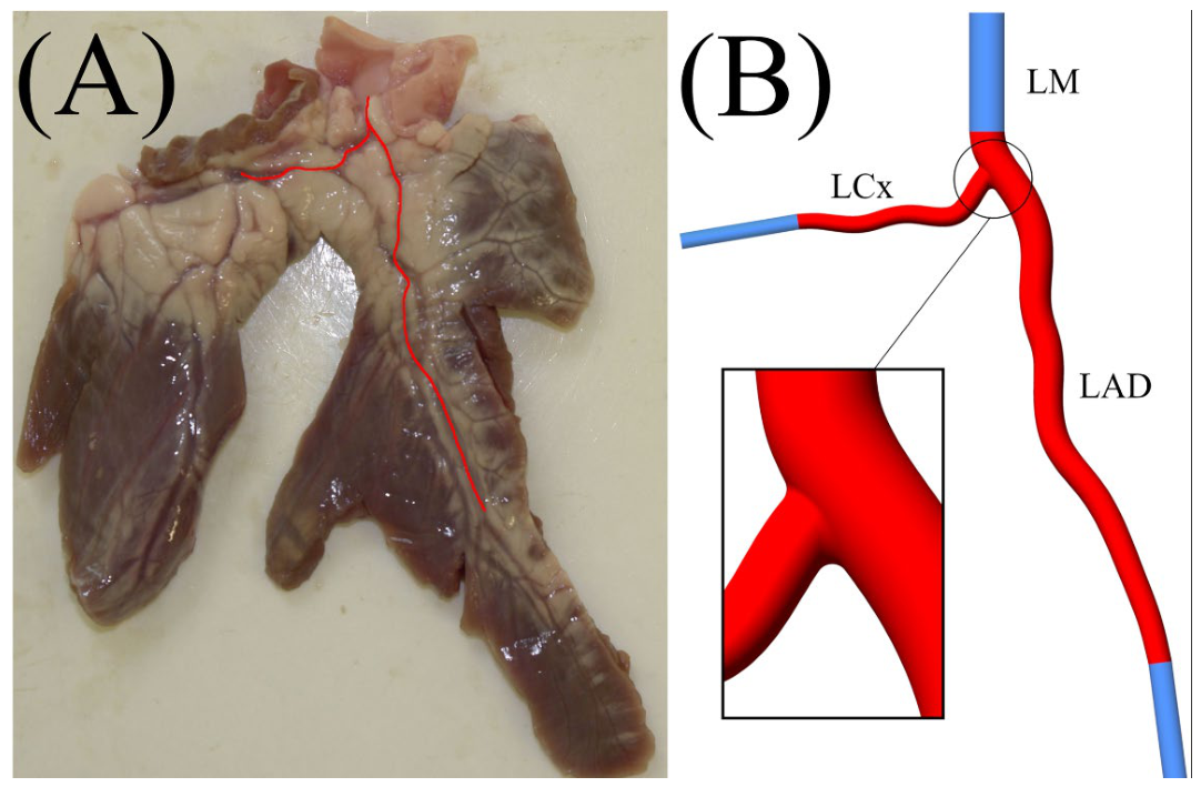
Figure 1. “(A)—Porcine ex vivo heart segment, with coronary geometry marked in red. (B) Coronary artery bifurcation geometry including domain extensions shown in blue (LAD, left anterior descending artery; LCx, left circumflex artery; LM, left main coronary artery).” This text and figure have been reproduced from Reference [19], which is distributed under the terms of the Creative Commons Attribution 4.0 International License (http://creativecommons.org/licenses/by/4.0/ (accessed on 10 May 2026)), which permits unrestricted use, distribution, and reproduction in any medium. Note: In the remainder of the manuscript, the left main coronary artery is referred to as LMCA.
Fluids 11 00118 g001
Figure 2. Coronary artery modelling. (A) Healthy coronary artery replicated in ANSYS. (B) Stenosed coronary artery replicated in ANSYS. (C) Velocity waveform for coronary artery [30]. LMCA refers to left main coronary artery; LAD to the left anterior descending artery; and LCX to the left circumflex artery.
Fluids 11 00118 g002
Figure 3. Meshing. (A) Mesh convergence analysis across 6 mesh sizes, where orange refers to peak outlet velocity and blue to mean velocity. (B) Meshed geometry for stenosed model.
Fluids 11 00118 g003
Figure 4. Data-driven and physics-informed data-driven neural network architecture.
Fluids 11 00118 g004
Figure 5. Physics-informed neural network architecture.
Fluids 11 00118 g005
Figure 6. Calculating wall distance.
Fluids 11 00118 g006
Figure 7. CFD predictions for flow through a coronary artery bifurcation. For a stenosed artery, evaluating: (A) WSS for geometry A69.5S50I4.5O3.0, (B) WSS for geometry A82.5S50I4.5O3.0, and (C) velocity for geometry A69.5S50I4.5O3.0. For an otherwise ‘healthy’ artery, evaluating: (D) WSS for geometry A69.5S0I4.5O3.0, (E) WSS for geometry A82.5S0I4.5O3.0, and (F) velocity for geometry A69.5S0I4.5O3.0.
Fluids 11 00118 g007
Figure 8. CFD and data-driven ANN u velocity predictions for geometry A72.5S0I4.5O3.0. (A) CFD u velocity heat map. (B) ANN prediction u velocity heat map. (C) Error plot for u velocity prediction by data-driven ANN.
Fluids 11 00118 g008
Figure 9. CFD and data-driven ANN v velocity predictions for geometry A72.5S0I4.5O3.0. (A) CFD v velocity heat map. (B) ANN prediction v velocity heat map. (C) Error plot for v velocity prediction by data-driven ANN.
Fluids 11 00118 g009
Figure 10. CFD and data-driven ANN VF predictions for geometry A72.5S0I4.5O3.0. (A) CFD VF velocity heat map. (B) ANN prediction VF velocity heat map. (C) Error plot for VF velocity prediction by data-driven ANN.
Fluids 11 00118 g010
Figure 11. Error plots (%) for velocity predictions by the data-driven ANN, for the stenosed geometry A80.5S50I4.5O3.0. (A) u error. (B) v error.
Fluids 11 00118 g011
Figure 12. CFD and data-driven ANN VF predictions for the stenosed geometry A80.5S50I4.5O3.0. (A) CFD VF velocity heat map. (B) ANN prediction VF velocity heat map. (C) Error plot for VF velocity prediction by data-driven ANN.
Fluids 11 00118 g012
Figure 13. CFD and PINN u velocity predictions for the stenosed geometry A77.5S50I3.9O2.9. (A) CFD u velocity heat map. (B) PINN prediction u velocity heat map. (C) Error plot for u velocity prediction using PINNs.
Fluids 11 00118 g013
Figure 14. CFD and PINN v velocity predictions for the stenosed geometry A77.5S50I3.9O2.9. (A) CFD v velocity heat map. (B) PINN prediction v velocity heat map. (C) Error plot for v velocity prediction using PINNs.
Fluids 11 00118 g014
Figure 15. CFD and data-driven + ROM-PINN prediction of VF, for stenosed geometry A77.5S50I4.0O3.0, the ‘worst’-performing prediction. (A) CFD VF heat map. (B) Data-driven + ROM-PINN predicted VF heat map. (C) Error plot for VF prediction using data-driven + ROM-PINN.
Fluids 11 00118 g015
Figure 16. CFD and data-driven + ROM-PINN prediction of VF, for stenosed geometry A82.5S50I4.5O3.0, the ‘best’-performing prediction. (A) CFD VF heat map. (B) Data-driven + ROM-PINN predicted VF heat map. (C) Error plot for VF prediction using data-driven + ROM-PINN.
Fluids 11 00118 g016
Table 1. Geometry variations used for dataset. Where a range is provided, increments were in steps of 0.1 for diameters, and 1° for angles.
GeometryBifurcation Angle (°)StenosisInlet Diameter (mm) Outlet 1
Diameter (mm)
Outlet 2
Diameter
(mm)
1–2466.5–89.50%4.53.52.5
25–4866.5–89.550%4.53.52.5
49–6477.50%3.5–52.5–42.5
65–8077.550%3.5–52.5–42.5
Table 2. Mesh quality evaluation, where Avg. refers to mean average, and Max. to maximum.
Elements Average Skewness Maximum
Skewness
ANSYS
Maximum
Skewness
Average
Orthogonality
Minimum
Orthogonality
ANSYS
Minimum
Orthogonality
Avg.
Aspect
Ratio
Max.
Aspect
Ratio
Max.
Avg.
ANSYS
Ratio
109,9600.210590.767090.950.788210.232910.11.8071 7.903 5
208,5270.209460.798810.950.789280.201190.11.8074 8.377 5
498,3210.20970.799780.950.789090.200220.11.8072 8.7818 5
784,9080.221280.799510.950.777330.200490.11.8346 9.6467 5
979,5270.214090.796710.950.784590.203290.11.8182 8.5087 5
1,043,6590.212820.79580.950.785880.20420.11.815 8.751 5
Table 3. Wall-clock simulation time for transient and steady-state runs.
Simulation Type Time-Step (s)Minimum Time
(Hours)
Maximum Time
(Hours)
Average Time
(Hours)
Transient0.00168.2276.3570.3
Steady-StateN/A0.631.20.8
Table 4. Neural network models and total predictions made.
ModelNumber of Geometries Trained onPredictions Made from Each ModelNumber of Geometries
Predicted
Data-Driven ANN80u, v, VF40
PINNs5u, v5
PINNs into Data-Driven ANN80VF20
Table 5. Data-driven neural network set-up. Note: The learning rate was experimentally tuned based on performance for each specific dataset.
InputModel
Architecture
OutputLoss
Function
Generalisation
Spatial coordinates (x, y)
Angle of bifurcation (θ) Diameter of the inlet and outlet 1 (Figure 2) (øI, øo)
Wall distances (Wd1, Wd2)
Stenosis (S)
10 layers of 32 neurons utilising the ReLU activation function, ran for 10,000 epochs and batch size 128 with an early stop of patience 150. Trained using the Adam optimiser. Volume fraction
(VF)
Velocity in x direction (u)
Velocity in y direction (v)
Mean
squared
error (MSE)
loss
Drop-out layers added for each layer. A 0.1 rate (i.e., 10% drop-out) for the first 5 layers and 0.2 (i.e., 20% drop-out) for last 5 layers.
Batch normalisation applied between each layer
Table 6. Physics-informed neural network set-up.
InputModel
Architecture
OutputLoss Function
Spatial coordinates (x, y) 12 layers of 128 neurons utilising the sigmoid activation function, ran for 2500 epochs with batch size 256. The Adam optimiser was used for training all ANNs. The initial learning rate was 10−3, reducing during later epochs based on the loss function performance [24].Velocity along x direction (u)
Velocity along y direction (v)
Partial Differential Equation Loss—Navier–Stokes equations
Boundary Condition Loss—Input the wall boundaries by explicitly defining the x and y coordinates where the u and v velocities are zero
CFD Sparse Data Point Loss—5 data points from the test data that allow the PINN model to converge better
Table 7. CFD validation against studies from literature. For generated data, the file name uses a format of ‘Axx.xSxxIx.xOx.x’, whereby the angle of bifurcation is given by A (followed by the angle, as measured in °), stenosis is denoted by S, the inlet diameter is noted as I (followed by the diameter, as measured in mm) and outlet diameter as O (followed by the diameter, as measured in mm).
Source MethodStenosisMean Velocity
(ms−1)
Max
Velocity
(ms−1)
Mean WSS
(Pa)
Max WSS
(Pa)
Generated Data
A69.5S0I4.5O3.0
CFDNormal0.2200.5011.867.87
Generated Data
A82.5S0I4.5O3.0
CFDNormal0.2170.4991.887.04
Generated Data
A69.5S50I4.5O3.0
CFDStenosed0.2510.8232.17916.60
Generated Data
A82.5S50I4.5O3.0
CFDStenosed0.2440.8112.1816.71
Study [53]CFD
Clinical
Literature-
Based
Normal--0.75–2.255.82–7.04
Study [54]CFDNormal--1–7<7
Study [55]CFD-MRINormal--1.26–2.69<2.7
Study [56]CFDStenosed--1.0–2.510–42
Study [57]CFDStenosed--<2.55.2–30.3
Study [58]FFR & FD-
OCT
Stenosed0.223 ± 0.023-
Study [52]DopplerStenosed-0.9 ± 0.32--
Study [51]DopplerNormal and
Stenosed
0.32 ± 0.170.89--
Study [51]DopplerNormal0.27 ± 0.160.43--
Study [51]DopplerStenosed0.33 ± 0.200.53--
Table 8. Data-driven ANN prediction of velocity for two of the 40 geometries solved. The † ‘best’ and ‡ ‘worst’ predictions are reported. Mean squared error: MSE; average percentage error: APE; u: velocity along the x-axis as shown in figures; v: velocity along the y-axis as shown in figures; VF: volume fraction.
Geometryu MSE (m/s)v MSE
(m/s)
VF MSE u APE
(%)
v APE
(%)
VF APE
(%)
‡ A70.5S50I4.5O3.0 0.0143 0.00846 0.00436 71.84 47.33 12.01
† A77.5S50I4.0O3.0 0.0103 0.00734 0.00680 51.12 35.30 15.23
Table 9. PINN prediction of velocity for two of the five geometries solved. The † ‘best’ and ‡ ‘worst’ predictions are reported. Mean squared error: MSE; average percentage error: APE; u—velocity along the x-axis as shown in figures; v—velocity along the y-axis as shown in figures.
Geometryu MSE (m/s)v MSE (m/s)u APE (%)v APE (%)
‡ A69.5S0I4.5O3.04.04 × 10−31.92 × 10−38.516.98
† A77.5S50I3.9O2.93.93 × 10−31.86 × 10−36.125.63
Table 10. Data-driven and PINN prediction of volume fraction (VF) for three of the 20 geometries solved. The † ‘best’ and ‡ ‘worst’ predictions are reported. Mean squared error: MSE; average percentage error: APE.
GeometryMSEAPE (%)
‡ A77.5S50I4.0O3.0 1.108 × 10−60.0542
† A68.5S50I4.5O3.0 4.097 × 10−70.0415
Table 11. Runtime analysis calculated from 3 runs of each model.
Simulation TypeMinimum Time
(Hours)
Maximum Time
(Hours)
Average Time
(Hours)
CFD: Transient 68.2276.3570.3
CFD: Steady-State 0.631.200.8
Data-Driven Model 0.41671.450.783
PINNs 3.96675.094.35
Data-Driven and PINNs
Hybrid Model
4.4825.514.85
Disclaimer/Publisher’s Note: The statements, opinions and data contained in all publications are solely those of the individual author(s) and contributor(s) and not of MDPI and/or the editor(s). MDPI and/or the editor(s) disclaim responsibility for any injury to people or property resulting from any ideas, methods, instructions or products referred to in the content.