Abstract
Computational Fluid Dynamics (CFD) is regarded as an important tool for analyzing the flow field, thermal environment, and air quality around the built environment. However, for built environment applications, the high computational cost of CFD hinders large-scale scenario simulation and efficient design optimization. In the field of built environment research, surrogate modeling has become a key technology to connect the needs of high-fidelity CFD simulation and rapid prediction, whereas the low-dimensional nature of traditional surrogate models is unable to match the physical complexity and prediction needs of built flow fields. Therefore, combining machine learning (ML) with CFD to predict flow fields in built environments offers a promising way to increase simulation speed while maintaining reasonable accuracy. This review briefly reviews traditional surrogate models and focuses on ML-based surrogate models, especially the specific application of neural network architectures in rapidly predicting flow fields in the built environment. The review indicates that ML accelerates the three core aspects of CFD, namely mesh preprocessing, numerical solving, and post-processing visualization, in order to achieve efficient coupled CFD simulation. Although ML surrogate models still face challenges such as data availability, multi-physics field coupling, and generalization capability, the emergence of physical information-driven data enhancement techniques effectively alleviates the above problems. Meanwhile, the integration of traditional methods with ML can further enhance the comprehensive performance of surrogate models. Notably, the online ministry of trained ML models using transfer learning strategies deserves further research. These advances will provide an important basis for advancing efficient and accurate operational solutions in sustainable building design and operation.
1. Introduction
Airflow organization in the built environment not only directly affects the indoor and outdoor environmental quality, energy efficiency, and human comfort, but also is a key factor to protect the health of residents and achieve sustainable development [1,2]. Computational Fluid Dynamics (CFD) has become a fundamental tool for simulating fluid flow, heat, and mass transfer in these complex environments, which utilizes numerical methods to solve the governing equations in a large space and with high resolution [3,4].
With the diversification of building forms and functional complexity in the process of urbanization, engineering practice has put forward the urgent need for rapid decision-making and multi-scenario comparison for ventilation optimization, pollutant dispersion simulation, and wind load assessment in the built environment [5,6]. However, traditional CFD simulations usually involve time-consuming meshing, iterative solving of nonlinear equations, and high-performance computing resources [7]. This inherent limitation significantly restricts its rapid application and optimization efficiency in the early stage of engineering design.
Recently, the booming development of machine learning (ML) technology has provided a brand-new path to break through the bottleneck of CFD computational efficiency. The ability of ML to characterize system behavior in a data-driven manner enables a range of potential applications in science [7,8]. By utilizing a data-driven approach, ML algorithms excel at identifying latent patterns in high-dimensional fluid dynamics data, thus enabling surrogate models that bypass traditional numerical solvers [9,10]. Although the training phase of ML models can be time-consuming, they are very effective in making new predictions [11]. Applying ML to CFD simulation can greatly shorten the calculation time, enabling the originally time-consuming complex airflow simulation to obtain approximate but sufficiently accurate results in a shorter time [12,13]. It provides strong support for rapid decision-making and optimized design in engineering practice.
ML-based surrogate models can predict the flow field around a building in milliseconds to seconds by deep training on CFD data, realizing tens to hundreds of times efficiency gains compared to traditional CFD methods [14,15,16]. The Artificial Neural Network (ANN) model is highly adaptable and can be applied to different scenarios ranging from ventilation analysis to pollutant dispersion prediction, while maintaining fidelity comparable to traditional CFD in many real-world scenarios [17,18]. Crucially, such models enable rapid feedback loops for design optimization and operational control.
This review focuses on rapid CFD prediction techniques based on ML surrogate models in the built environment domain. Unlike other reviews, it not only provides a comprehensive overview of various methods, models, and application examples of ML for CFD acceleration in this domain, but also analyzes the applicability and limitations of different surrogate models in different built environment scenarios. Section 2 introduces the basic principles of CFD and its engineering applications in the built environment. Section 3 explores the traditional surrogate modeling and ML approaches used to accelerate the CFD workflow. Section 4 elaborates the framework of ML accelerating CFD, focusing on how ML accelerates strategies at each stage of CFD simulation. Section 5 focuses on the engineering application of using ML to achieve rapid prediction in the built environment.
2. CFD for the Building Environment
2.1. Typical Applications of CFD in the Building Environment
CFD is a high-fidelity modeling method based on detailed physical principles that can successfully make detailed predictions of various airflow and temperature distributions [19]. Fluid motion is usually divided into two typical flow regimes, laminar flow and turbulent flow. In the built environment, the flow field is usually turbulence-dominated. This phenomenon is attributed to the multiphysical coupling mechanism, which includes high Reynolds number flow conditions, geometrical complexity of the building form, and the synergistic effect of atmospheric turbulence on the incoming flow characteristics [20]. The temporal and spatial non-constant properties of turbulence significantly affect the wind load distribution, indoor and outdoor ventilation efficiency, and pollutant diffusion and transport in building structures, which is the core scientific issue in building environmental engineering [21].
Currently, CFD simulation methods for turbulent air flow fields consist of three main categories: direct numerical simulation (DNS), large eddy simulation (LES), and Reynolds Average Navier–Stokes (RANS) simulation using turbulence models. LES and RANS methods have been widely adopted for rapid computational analysis of turbulent flows. While LES offers higher accuracy than DNS by resolving large-scale eddies and modeling small-scale turbulence, its computational cost remains significantly higher than RANS due to the explicit resolution of transient flow features. In the context of RANS, two-equation turbulence models, including the k-ε and k-ω frameworks, are commonly employed to predict fluid field variables [22]. Among these, the k-ε model has demonstrated broader applicability and robustness in diverse engineering scenarios, particularly in steady-state simulations with well-defined boundary conditions [23]. However, its performance may degrade in complex flows with strong adverse pressure gradients or separation phenomena, necessitating careful validation for specific applications.
2.2. Engineering Applications of CFD in the Built Environment
Numerous applications of the built environment are closely related to the study of fluid flow, which not only covers the micro-environment inside buildings but also includes large-scale flow fields in the external urban canopy [24,25,26]. For instance, indoor environments have the core design goals of ensuring occupant comfort and maintaining satisfactory indoor air quality, while outdoor simulation focuses on the behavior of external airflow in the built environment [27,28,29,30,31].
CFD techniques are widely used for modeling indoor environments, covering complex ventilation systems and thermal comfort simulation studies [32]. Its excellent simulation capabilities provide a solid theoretical basis and an effective analytical tool for indoor environmental quality studies by accurately modeling key physical processes such as airflow, heat transfer, and particle dispersion [33,34]. In terms of further deepening the application of CFD technology, an in-depth study of the interaction between the indoor environment and the human thermoregulation system can be realized by integrating it with the human thermoregulation model (Figure 1) [35]. As a neighborhood-scale modeling tool, the effectiveness of CFD has been fully confirmed [36,37,38,39,40]. Pedestrian wind comfort is a traditional problem in outdoor built environments during the study of average speeds in high-speed areas around buildings (Figure 2) [41]. Since the inception of CFD technology, the extensive history of its application in the built environment has been emphasized in numerous literature reviews, which fully proves the key role and irreplaceability of CFD in this field [41,42,43].
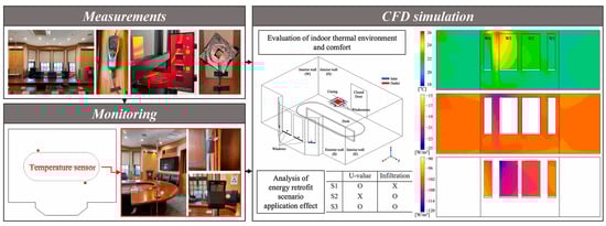
Figure 1.
Indoor thermal environment assessment of historic buildings using CFD, extracted from Kang et al. [35].

Figure 2.
Evaluating urban wind fields using CFD, modified from Zhao et al. [41]. (a) Urban spatial layout. (b) Pedestrian-level turbulent kinetic energy.
2.3. CFD Challenges in Built Engineering
Current CFD models have achieved effective handling of most flow physics problems in the built environment, including indoor and external flow phenomena [44]. The key challenge in applying CFD to build environment systems is the high computational cost, particularly in scenarios requiring rapid optimization or multi-scenario comparisons. This cost arises from two main factors: (1) the need for fine meshes in complex geometries (e.g., building façades, ventilation ducts), and (2) the use of high-fidelity turbulence models (e.g., LES, Low Reynolds Number models) to resolve transient flow features. In order to accurately capture these complex phenomena, CFD requires the generation of fine computational grids, especially in areas with complex geometries, where the number of grids tends to grow exponentially. In addition, in CFD simulation, each source requires different boundary conditions based on its characteristics. Since a small release area leads to a high concentration gradient in the local space near the point source, this high concentration gradient can significantly slow down the convergence of the computational process if the simulation is to capture this phenomenon. Although the use of LES and Low Reynolds Number models is theoretically possible to obtain more accurate results, it requires a lot of computational resources and time, which can take hours to days for a single full simulation [45,46]. Furthermore, CFD requires multi-core/cluster resources for multi-scenario optimization, and there is a linear relationship between resource scale and cost.
The above issues make it difficult to apply traditional CFD in scenarios such as rapid optimization of the built environment and rapid comparison of multiple scenarios. The introduction of the ML surrogate model provides an effective solution to these problems and opens up new avenues for research and practice in the field of the built environment.
3. Rapid Prediction Methods Based on CFD
This section systematically describes the rapid prediction techniques based on traditional surrogate models, ML, and ANN, comparing their principles, application scenarios, and limitations. It provides a valuable reference for beginners to adopt Artificial Intelligence (AI) to solve fluid dynamics problems in the built environment. ML is a large class of AI that contains various algorithms such as Random Forest (RF), Principal Component Analysis (PCA), and Neural Networks. Among them, neural networks are an important subset. Surrogate models for approximating complex systems or processes can be constructed using both traditional mathematical methods and ML methods.
3.1. Traditional Surrogate Model
In the field of engineering optimization, traditional surrogate models are widely used as an efficient alternative to complex numerical simulations to reduce computational costs and speed up the design process. Common surrogate models include polynomial regression, response surface modeling, and Kriging model [47,48,49]. Response surface models fit the input-output relationship by polynomials and are suitable for rapid approximation of low-dimensional problems, but their accuracy is limited in high-dimensional nonlinear issues [50]. The Kriging model is based on Gaussian processes and models sample correlations through covariance functions. It can provide prediction error estimates through spatial interpolation and shows high robustness in aerodynamic optimization. However, its computational complexity increases significantly with the increase of the sample size [51,52].
However, the performance of traditional surrogate models is highly dependent on the number and distribution of training samples; a small number of samples may lead to prediction bias, and the cost of generating high-fidelity samples may still constrain their application [53]. Moreover, as the input parameters increase, the sample requirement grows exponentially, the fitting accuracy of low-order models decreases, and the computational complexity of high-order models (e.g., RBFs) soars. In addition, in multi-objective optimization, the trade-off relationship between conflicting objectives needs to be handled. Traditional methods often convert multi-objectives into single objectives through weighting functions, but the selection of weights relies on experience and may affect the diversity of solutions [54,55].
Recently, with the evolution of technology, ML-based proxy models have relied on data-driven modeling methods. It can effectively overcome the inherent limitations of traditional proxy models in terms of sample dependence, dimensional scalability, and multi-objective processing, and gradually become the core method for accelerating CFD simulation at present.
3.2. ML-Based Surrogate Model
3.2.1. ML Method
The core principle of ML is to train the proxy model using large-scale original datasets. After the successful completion of the training, the model can achieve excellent computational efficiency and accuracy [56,57]. Notably, this computational advantage provides significant opportunities for accelerating numerical simulation of fluid dynamics, especially for complex flow phenomena that traditionally require resource-intensive CFD methods. ML is classified into three main learning paradigms based on the utilization of the data and the learning objectives, with multiple algorithms for each paradigm, shown in Figure 3.
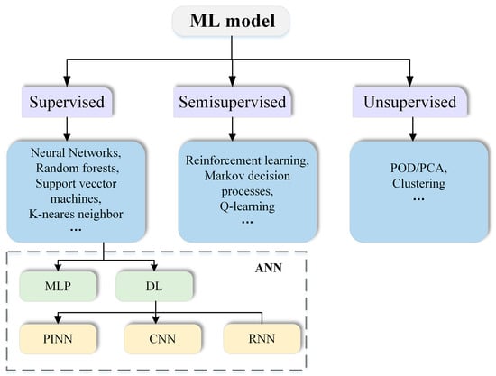
Figure 3.
Schematic diagram of ML classification.
- Supervised learning trains a model with input features and corresponding output labels. For example, taking CFD geometric parameters or boundary conditions as inputs and flow field data as outputs, a model is trained to predict the response of future observations [58]. In this way, unknown flow fields can be predicted quickly without conducting new simulations.
- Unsupervised learning analyzes unlabeled data, allowing the discovery of the intrinsic structural properties of the data based on input features alone through techniques such as clustering, quantization, and dimensionality reduction [59]. For example, POD methods can be used to downscale the Navier–Stokes equations by constructing Galerkin projections on the respective modes, while combining a discretized form of the energy equation with a state-space model for systematic integration [60].
- Semi-supervised learning combines a small amount of labeled data with a large amount of unlabeled data to train models [61]. When the sample size is limited, semi-supervised regression is used to construct pseudo-labeled samples of untested building groups and mix them with existing samples to expand the sample size [62].
Unsupervised and semi-supervised learning can reduce the reliance on data labeling and assist in accelerating the solution, which, however, is not as direct as supervised learning and needs to be combined with supervised learning to achieve rapid prediction in CFD.
3.2.2. ANN Method
ANN, as a major method in the supervised learning framework, has been widely used in fluid mechanics. Attention is drawn to the fact that this architectural advantage confers ANN with superior performance in solving nonlinear issues compared to traditional ML models. In 1986, Rumelhart et al. [63] reintroduced and refined the backpropagation algorithm (BP), which enabled efficient parameter optimization in multilayer networks. This advancement spurred research efforts to integrate neural networks with fluid dynamics. In this section, a systematic description of the fundamentals of four representative neural network architectures, MLP, CNN, RNN, and PINN, which are often used to accelerate CFD prediction in built environment applications, is presented.
MLP is the most standard and common feedforward neural network, and also the infrastructure of deep learning. As shown in Figure 4a, it is the simplest MLP structure, consisting of two input nodes, a single hidden node, and a single output node. Some early studies attempted to use MLP to make preliminary predictions of the flow field around buildings. However, due to the relatively simple structure of the MLP model, its ability is limited when dealing with data with spatial correlation and complex structure. With the deepening of research, its application has gradually been replaced by more advanced deep learning models.

Figure 4.
Schematic diagram of a typical ANN structure. (a) Schematic of the simplest MLP structure. (b) Example diagram of a CNN with 3 × 3 convolutional kernels. (c) Schematic of the basic RNN structure. (d) Schematic of PINN structure with physical control equations embedded in the neural network. (Blue nodes represent input layers, green nodes represent hidden layers, and purple nodes represent output layers).
CNN uses convolution to automatically extract local features from data, and its predecessor is LeNet, which was started as a handwritten digit recognition network. However, due to the constraints of computer hardware and equipment, CNNs have only been widely studied in image classification and object detection after 2012 [64]. Since CNN can efficiently capture the spatial pattern and structure of the flow field, it has been applied to study the flow field distribution in the built environment. Jin et al. [65] utilized CNN to identify the pressure values on a cylinder to predict the velocity field. As shown in Figure 4b, the CNN extracts the hierarchical features of the flow field through multilayer convolution and pooling operations, which in turn enables the prediction of physical quantities such as pressure distribution and velocity field. However, the pooling operation may lose part of the location information, which requires additional design for tasks requiring accurate spatial localization.
RNN is mainly used to process data with time series, which stores past information by introducing memory units [66], as shown in Figure 4c. In CFD prediction of the built environment, the movement of fluids has temporal characteristics, such as wind fields and temperature fields that change over time. Lee et al. accurately predicted urban boundary layer dynamics and transient turbulence by modeling the temporal evolution of fluid motion using a circulation structure within the RNN [67]. However, traditional RNNs suffer from the problems of gradient vanishing and gradient explosion, and have limited effectiveness in dealing with long sequence data [68]. Therefore, Long Short-Term Memory networks (LSTM) with special gating mechanisms were proposed in 1997 [69]. LSTM is an improved RNN structure that can better capture long-distance temporal dependencies and has been increasingly applied in CFD prediction tasks where the building environment changes over time.
PINN is a neural network model that has emerged in recent years, proposed by Raissi et al. It is considered an efficient solver for partial differential equations [70]. It can embed the equations of the physical control of the fluid (e.g., NS equations) into the loss function of the neural network, as in Figure 4d. Wei et al. [48] used measured data as inputs to the PINN to reconstruct the detailed 2D airflow field without inlet boundary conditions. Moreover, it saves 42% of the computation time compared with the traditional CFD, which effectively compensates for the traditional data-driven method’s over-reliance on data and neglect of physical laws. However, the loss function of PINN contains multiple competing terms, which are difficult to balance, and the optimization process is complicated and prone to falling into local minima or difficult to converge.
Overall, each model has its own characteristics and applicable scenario models. Researchers should select the appropriate model based on specific practical problems.
4. ML Accelerated CFD Frameworks for Rapid Prediction
The integration of ML technology into CFD predictions for the built environment is increasingly expanding and deepening, offering robust support for accelerating CFD simulations and enhancing the understanding of fluid phenomena within architectural settings. This section provides a systematic review of the development of coupling frameworks between CFD and ML, as well as the application of ML techniques to accelerate critical stages of CFD simulations.
4.1. CFD-ML Coupled Model Basic
Although CFD solvers have evolved into a well-established system over several decades, the deep integration of ML with traditional numerical simulation methods remains in its infancy [71]. Caron et al. [72] highlighted that it is impractical for ML to entirely replace CFD in the near future. Consequently, a more feasible strategy involves constructing a coupled framework of CFD and ML, leveraging ML models to either model or optimize the complex physical processes within CFD simulations. This approach not only reduces computational time but also enhances simulation efficiency.
The coupling of CFD and ML primarily manifests in two distinct paradigms. One involves embedding ML models within the architecture of CFD solvers to enhance and accelerate traditional numerical methods [73,74]. The underlying principle is to leverage data-driven models as substitutes for specific physical modeling components. McConkey et al. [75] predicted the linear and nonlinear parts of the Reynolds stress tensor based on a neural network embedded in the tensor decomposition, with velocity field prediction accuracy exceeding that of conventional physical models. Geneva et al. [76] addressed the problem of quantifying uncertainty in data-driven turbulence models by proposing a new framework that improves RANS predictions while providing probabilistic bounds on the flow field variables to enable quantitative measurement of model form and cognitive uncertainty. The other paradigm involves the independent operation of CFD and ML models, with computational efficiency enhanced through data interaction. Specifically, CFD generates high-quality training datasets to support the training of ML models, while the trained ML models enable rapid prediction of flow field characteristics in new scenarios [77,78]. This approach establishes a synergistic mechanism between CFD and ML via data exchange, significantly boosting computational efficiency while maintaining prediction accuracy. Vandewiel et al. [79] showed that a post-trained CNN surrogate model could approximate RANS simulations of natural ventilation within a few milliseconds (Figure 5). Liu et al. [80] combined the Kriging surrogate model to achieve fast IAQ prediction under limited samples and dynamically adjusted the ventilation strategy through an optimization algorithm.
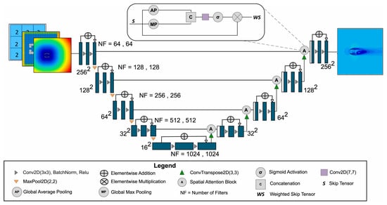
Figure 5.
Spatial Attention CNN surrogate model, extracted from Vandewiel et al. [79].
4.2. ML Accelerated CFD Simulations
A typical CFD simulation consists of the following key steps: first, a 3D model is constructed to generate a computational grid. Then, based on the conservation law of momentum, the temporal and spatial changes of the fluid in each grid cell are solved. Finally, the simulation results are visualized. This section will systematically sort out the research progress and cutting-edge applications of ML to realize targeted accelerated CFD in the key aspects of mesh preprocessing, numerical solving, and post-processing.
4.2.1. ML for Preprocessing
In the CFD preprocessing stage, mesh generation is significantly more time-consuming than geometric modeling. Geometric modeling typically relies on readily available design drawings or models, making it relatively efficient. In contrast, mesh generation must satisfy stringent requirements for mesh quality and resolve the complex flow fields surrounding buildings through fine discretization. Moreover, the high-resolution demands of turbulence simulations result in a substantial increase in mesh density and necessitate repeated iterative optimization. Consequently, this section focuses on summarizing the research progress in leveraging ML techniques to accelerate mesh generation.
Since the 1990s, ML technology has progressively exhibited distinct advantages in finite element mesh generation and adaptive optimization, driving the innovation and advancement of computational methodologies. Early studies (1996–1997) pioneered the mapping of mesh partitioning problems onto ML network models, enabling the automatic generation of node topological structures via coordinate allocation [81]. This type of approach maps the mesh partitioning problem to a neural network, and optimizing the node positions significantly improves the accuracy of the numerical solution, while reducing the dependence of traditional mesh partitioning on manual experience [82]. Over time, researchers began to investigate the application of neural networks in dynamic scenarios [83]. Manevitz et al. [84] used neural network methods for time series prediction to obtain effective mesh refinement at the appropriate time. In the two-dimensional wave equation, the coarse mesh is taken as the input, and the model is run to control the insertion of the new mesh. This prediction-based adaptive strategy achieved superior accuracy compared to traditional post-processing error estimation methods under equivalent computational resources.
In recent years, neural networks have achieved continuous and significant advancements in the field of finite element mesh generation and optimization [85,86]. Guo et al. [87] proposed a novel approach fusing heuristic and optimization smoothing. The model takes the ring formed by the neighboring nodes of a free node as input, predicts the optimal position of the free node, and optimizes the mesh by moving the node directly without changing the mesh topology. ML-driven techniques for predicting mesh spacing functions [88], such as the Implicit Geometry Neural Network (IGNN), enable the automated generation of adaptive meshes by learning the mapping between geometric characteristics and mesh size functions (Figure 6) [89]. Meanwhile, 3DMeshNet embeds the differential equations for mesh generation into the loss function of the neural network and learns mappings in the space with geometric points as inputs to achieve fast generation of 3D structured meshes. These approaches have exhibited remarkable robustness and efficiency across various scenarios, achieving an 85% reduction in mesh generation time and a 4- to 8-fold decrease in computational costs [90].
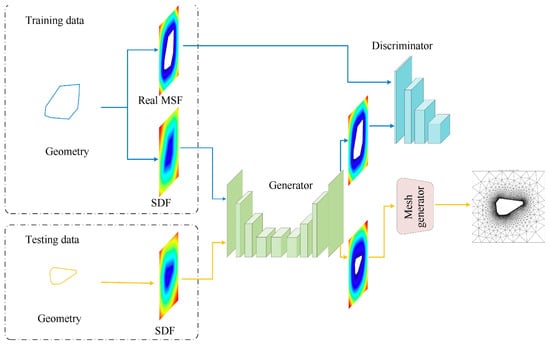
Figure 6.
Flowchart of adaptive mesh generation, modified from Xu et al. [89].
4.2.2. ML for Numerical Solution
Numerical solution constitutes the core component of CFD simulations, entailing a substantial number of computational operations [91]. In this context, ML primarily contributes to accelerating the solution process and enhancing solution accuracy. Some studies focus on leveraging ML models to either fully or partially substitute traditional numerical solvers. Notably, research has concentrated on the pressure solver, a computationally intensive module [92,93]. Sousa et al. [94] integrated an ML surrogate model with an incompressible fluid solver to create two ML-enhanced CFD solver variants (Figure 7), which effectively reduced the number of iterations of the pressure solver in unsteady flow simulations. The simulation results in key metrics, such as drag coefficients and Strouhal numbers, are substantially reduced by about eight times in execution time compared to the conventional method. Yousif et al. [95] reconstructed the flow field obtained from DNS back to its original resolution based on a convolutional autoencoder. Then, an LSTM model of predicted fluid flow was used to predict the time evolution of low-dimensional data, and the turbulent pulsation characteristics at the DNS level were successfully reproduced with the statistical properties and energy spectrum errors below 3%. Ling et al. [72] proposed using neural networks to learn the Reynolds stress anisotropy tensor model from CFD data. This method ensures the rotational invariance of tensor eigenvalues, and the prediction error of the velocity field in complex flows is significantly reduced compared with the traditional vorticity model.
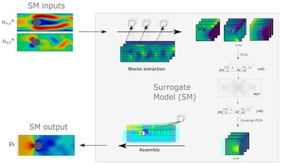
Figure 7.
Surrogate model graphical representation, extracted from Sousa et al. [94]. The input of SM is the longitudinal ux,t* and vertical vy,t* components of the velocity field at time t, while the sole output is the predicted pressure field pt at time t.
Meanwhile, ML can also be employed to enhance the algorithms and models for numerical solutions [96,97,98]. Calzolari et al. [99] integrated OpenFOAM with a data-driven zero-equation model based on deep learning, showcasing improved robustness and computational efficiency. In built environment simulations, this approach achieved a local pressure prediction speed 30 times faster than the traditional RANS method. Additionally, decoupling the Reynolds stress into linear and nonlinear components and predicting it through the completeness basis derived from the mean flow tensor helps overcome the ill-conditioning of the RANS equations [73]. Sousa et al. [100] developed an ML-based pressure solver that addressed the computational bottleneck of solving the Poisson equation via geometrically adaptive domain decomposition. Using an MLP-principal component analysis network, they achieved a 30-fold acceleration in local pressure prediction with a 3% error rate. Furthermore, by employing an end-to-end deep learning framework, they achieved 8–10 times spatial super-resolution in 2D turbulent flow simulations, accompanied by an 80-fold acceleration in computation.
4.2.3. ML for Post-Processing Visualization
CFD simulations produce vast amounts of data, and post-processing visualization plays a critical role in understanding and analyzing flow field results. Traditional post-processing methods demand manual parameter and threshold setting, which is not only inefficient but also highly reliant on user expertise. ML offers an automated and intelligent approach to post-processing visualization, specifically enabling data dimensionality reduction, visualization generation, and the automatic identification of key flow field features from CFD simulation results.
ML is capable of performing dimensionality reduction on large-scale flow field data. By retaining the primary feature information, it effectively reduces data complexity, thereby enhancing the efficiency and smoothness of the post-processing visualization process. Typical application scenarios involve unsupervised learning models, such as autoencoders (AE), which are able to map high-dimensional flow field data into a low-dimensional space while preserving key features [101]. Carlos et al. used high-fidelity flow field data, and the recirculation area and boundary conditions were identified through the ML model to identify the three-dimensional flow of the vortex at the junction. This method can distinguish the similar characteristics of fluids without a clear physical definition [102]. ML can automatically adjust visualization parameters, including color mapping, contour intervals, and vector graph density, according to the specific requirements of different users, thus generating visualization images that better align with user expectations. In terms of visualization generation, typical applications include the use of generative adversarial networks (GANs) to produce high-quality visualization images based on input flow field data [103]. Moreover, ML can be employed to automatically identify critical features in the flow field, such as vortices and boundary layers [104,105]. Typical applications include training with supervised learning models based on a large amount of labeled flow field data to learn automatic recognition patterns of common flow field features in the built environment, such as vortex areas, separation lines, and temperature areas [106]. Kashir et al. used CNN to convert each unit of the computational domain of CFD into the smallest possible measurement frame (Figure 8) to extract various features in the fluid flow. This method is particularly suitable for large-scale computing simulations with a large number of non-uniform grids [107].

Figure 8.
Schematic of CNN structure proposed by Kashir et al. [107,108].
The advancement of ML technology facilitates researchers in analyzing and interpreting CFD simulation results from multiple perspectives and at different levels, thereby offering stronger support for the optimization of building environment design.
5. ML Applied to Rapid Prediction of Built Environment
Combining ML with CFD to predict flow fields in the built environment offers a promising avenue for increasing simulation speed while maintaining reasonable accuracy. Through approximating complex physics-based CFD simulations, ML-assisted modeling allows for rapid prediction of airflow patterns.
5.1. Building Environment Surrogate Model
In the field of built environment research, surrogate modeling has emerged as a key technology to bridge the need for high-fidelity CFD simulations with the need for rapid predictions [109]. Surrogate models play a vital role in the rapid prediction of various parameters such as thermal comfort and air quality indoors, and wind fields and pollutants outdoors. Surrogate models utilizing ML algorithms learn patterns and relationships between various parameters from large data sets generated by high-fidelity CFD simulations or experiments [110]. Once trained, these surrogate models are able to approximate the output of complex physical processes at significantly lower computational cost (typically by several orders of magnitude) [111,112]. Surrogate models for the built environment focus on these three types of approaches: reduced order model (ROM), direct surrogate model (DSM), and ROM coupled with DSM.
ROM extracts the principal mode of the fluid dynamics equation through dimensionality reduction techniques, builds a low-dimensional model, and quickly predicts the flow field characteristics under different building layouts [113,114]. The fundamental work of POD in flow modal analysis dates back to Lumley 1970. After more than 50 years of theoretical refinement and engineering practice, the method has been expanded and applied to a variety of flow scenarios [115]. Typical applications include indoor temperature, particle concentration, and pressure [102,116,117,118]. Liang et al. [49] optimized the ventilation parameters and oxygen supply concentrations of plateau buildings calculated by CFD using POD, which improved the thermal comfort of personnel in the indoor environment of the plateau.
DSM is suitable for design space exploration and multi-objective optimization by directly mapping input parameters with outputs through algorithms such as neural networks and random forests. Deep learning architectures (e.g., CNN, RNN) dominate the surrogate model. Calzolari et al. [119] systematically illustrate the current state of the art of research on surrogate models in the construction field using a deep learning framework. It is pointed out that ANN can be used as an alternative solution to the traditional numerical simulation process or as a performance optimization module to achieve a rapid prediction of the building flow field while maintaining the prediction accuracy.
In the simulation of complex flow fields in the built environment, the single surrogate model faces the problem of accuracy degradation in multi-dimensional input space or insufficient computational gain due to insufficient dimensionality reduction. Therefore, the coupled modeling paradigm of ROM and DSM builds a hybrid surrogate model system with both physical mechanisms and statistical learning characteristics by synergistically integrating the dual advantages of dimensionality reduction technology and data-driven algorithms. The framework usually adopts a staged modeling strategy. Firstly, ROM is used to decompose the high-dimensional flow field data into intrinsic modes and extract the dominant spatiotemporal features. Subsequently, the DSM is employed to establish the nonlinear mapping relationship between the input parameters and the low-dimensional modal coefficients. Zhao et al. [25] used POD-ANN to predict indoor temperature by CFD simulation of the indoor flow field in a real school building as a case study (Figure 9). Under the premise of ensuring accuracy, this hierarchical decoupled modeling approach not only significantly reduces the input dimension of the neural network but also significantly improves the extrapolation ability of POD.
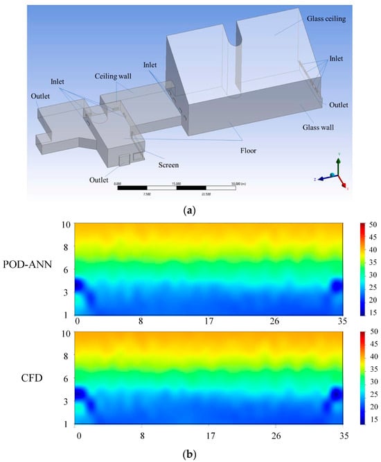
Figure 9.
POD-ANN predicts the indoor temperature field, modified from Zhao et al. [25]. (a) 3D model of a real school building. (b) Comparison of POD-ANN and CFD indoor temperature distribution results.
5.2. CFD-ML Rapid Prediction
ML models are trained to learn the mapping between input parameters and the resulting flow field characteristics of the building environment, including velocity vectors, pressure distributions, and turbulence parameter [108,120]. The ML surrogate model has been used in many studies in recent years to rapidly predict flow fields in indoor and urban environments of buildings, as shown in Table 1. This section focuses on the application of CFD-ML to realize rapid prediction of built environments from indoor and urban environments, respectively.

Table 1.
Recent research on the application of ML surrogate models in the built environment. Urban wind environment (UWE); Urban pollutants (UP); Indoor air quality (IAQ); Indoor environment (IE).
5.2.1. Internal Flow Field of Building
In research on CFD coupled with ML to realize rapid prediction of indoor environments, different ML learning models demonstrate unique advantages and usage scenarios. For example, Tian et al. [124] show that SVM can effectively predict the IAQ distribution of mixed ventilation under dynamic air supply parameter inputs by virtue of its global optimization property, which can avoid the overfitting problem that ANN is prone to, but its performance is highly dependent on the linear characteristics of the data Whereas Tian et al. [125] demonstrated that ANN can successfully predict multidimensional metrics such as energy efficiency and thermal comfort in stratified environments through nonlinear modeling capability, the purely data-driven ANN may lead to non-physical understanding due to the lack of physical constraints. With the deepening of research, PINN is embedded with physical conservation laws, such as the Navier–Stokes equations, as the loss function. Wei et al. showed that only a few spatial measurements are needed to reconstruct the 2D airflow field, which saves 42% of computation time compared with the traditional CFD and significantly outperforms the ANN when the data are sparse [48]. Xu et al. [126] revealed that the core watershed can be reconstructed even if the data sparsity is 1% or the core watershed data are missing. Research showed that the velocity and pressure fields can be accurately predicted even when the data sparsity reaches 1% or the core basin data are missing.
Moreover, when facing multivariate boundary conditions or highly dynamic time-series scenarios, the above models still face challenges. To this end, researchers have further introduced hybrid algorithmic architectures to expand the applicability boundaries of the coupled CFD-ML technique by compressing the problem dimensions or fusing the advantages of multiple networks. Wang et al. [123] developed a CNN-LSTM hybrid model integrating CFD data for the first time, which was used to efficiently predict human thermal comfort in indoor crowded environments (Figure 10). The model has high accuracy and stability in predicting dynamic indicators such as air velocity and temperature. The determination coefficient of the test set reaches 0.89, and it has good applicability to scenarios with high requirements for indoor time series data processing. Luo et al. [60] proposed that the POD-RBF model can quickly and accurately predict the indoor air temperature and velocity field, with a short construction and calculation time, with a small error, and is robust to low sampling volume, effectively reducing the burden of computation, suitable for rapid simulation of complex boundary conditions. GA-BP neural network with the help of genetic algorithms to optimize the initial weight of the BP network, the BP network’s prediction of the indicators of insufficient accuracy has been improved.
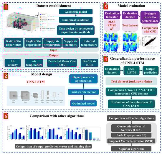
Figure 10.
CNN-LSTM coupling technology roadmap and results presentation, extracted from Wang et al. [123]. Subfigure 1 shows the dataset creation flowchart. Subfigure 2 shows the model building schematic of CNN-LSTM. Subfigure 3 shows the model evaluation. Subfigure 4 shows the generalization performance flowchart of CNN-LSTM. Subfigures 5 shows a comparison with other algorithms: (a) air flow rate, (b) air temperature, (c) PMV, and (d) DR.
5.2.2. External Flow Field of Building
The external flow field has a profound impact on factors including wind-induced pedestrian comfort, natural ventilation potential, and pollutant dispersion around the building. In the field of pollution in built-up urban environments, the combination of CFD and ML provides a powerful tool for responding to hazardous urban pollution events.
Kaloop et al. [127] compared and analyzed seven commonly used ML algorithms, such as feed-forward neural networks, RF, and DNN, in the field of predicting wind pressure in high-rise buildings and found that DNN performs optimally in predicting wind pressure in high-rise buildings through its nonlinear mapping ability, and its error is controlled at a low level in the training and testing stages. In addition, the strategy of directly utilizing CFD grid node data avoids the information loss of traditional image feature extraction and makes the prediction results more interpretable [47]. Wehrle et al. [122], the RF-based ML framework is able to efficiently map the morphological parameters to the mean wind speed by introducing 10 morphological parameters, revealing the key role of feature construction on model performance. The SEC hybrid framework integrates semi-supervised learning, extreme learning machine, and CFD simulation data, and alleviates the small-sample dilemma by constructing the pseudo-labeled samples. and its strategy of introducing the mean wind load as an auxiliary input cleverly reduces the nonlinear strength between inputs and outputs [62]. Its strategy of introducing the mean wind load as an auxiliary input subtly reduces the intensity of nonlinearity between the inputs and outputs. Remarkably, the Physical Information Graph Neural Network (PIGNN) achieves accuracy comparable to that of CFD on unstructured grids with 10–100 times computational speedup by embedding the RANS equations directly into the network architecture [128]. This physical constraint mechanism effectively solves the generalizability problem of purely data-driven models. The two-stage GNN framework, on the other hand, innovatively combines the steady-state RANS with the graph neural network to accelerate the convergence by utilizing the initial solution of coarse grid CFD, and achieves a computational efficiency 280 times higher than that of the traditional LES while maintaining the accuracy (Figure 11) [41].
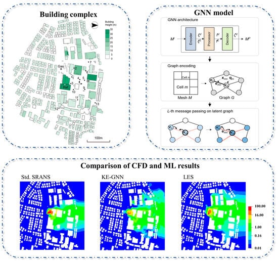
Figure 11.
GNN framework combined with graph neural networks, modified from Zhao et al. [41]. Numbers in the Building complex indicate measurement points.
As a surrogate model that can rapidly and accurately predict atmospheric pollution and dispersion, it needs to be both fast and physically plausible [129]. In order to achieve a fast and reliable assessment of air pollution exposure in urban areas, spatial constraints on topographic airflow and modeling the effects of analyzed obstacles are needed to estimate pollutant distributions [130,131]. The data-driven BPNN model is based on CFD data of multiple operating conditions to effectively capture the localization of pollutants on the leeward side of a building, which provides a microscopic scientific basis for the precise formulation of pollution control regulations. Huang et al. [132] established a spatial distribution dataset of pollutants through vehicle-mounted mobile monitoring experiments and used DL techniques to derive several urban morphology indicators from street view images. Despite the instability of the mobile monitoring data, the neural network was found to have the highest performance in predicting pollutant dispersion levels.
In summary, ML not only breaks through the limitations of traditional CFD methods in terms of computational cost and feature extraction, but also constructs a surrogate model system with both speed advantage and physical rationality through the deep integration of data-driven and physical mechanisms.
5.2.3. Calculation Time Advantages of CFD-ML
Numerous studies have shown that by training ML models on the data generated by CFD, accurate and physically consistent results can be quickly produced, thereby addressing the limitations of CFD methods in terms of long computing time [102,104,105,106,107,109,110,111,112,113,114,115,116,117,118,119,133]. In the simulation of building environment fluids, compared with the traditional CFD method, the CFD-ML strategy can achieve a reduction of orders of magnitude in computing time [108,121,122,123]. Zhao et al. [42] used POD coupled with ANN to predict indoor temperature. The research shows that POD-ANN can simultaneously take advantage of the strengths of both algorithms, reducing the computing time by 63% compared to traditional CFD simulation. Baitureyeva et al. [47] spent 1.5 months training the RF model using the RANS model to generate a CFD dataset of 300 urban wind environment cases. Under the same computing equipment, the training phase of the ML model was completed in just 30.4 s. Lin et al. [122,134] used the results of a verified turbulence model as the input of the BPNN model to study the diffusion characteristics of urban pollutants. After the model training was completed, the concentration distribution of NO could be collected in just a few seconds. Tian et al. [124] used 40 cases with different supply air parameters as the dataset of the BPNN model. The research shows that BPNN can almost instantly predict indoor thermal comfort while ensuring high data accuracy. This efficiency advantage enables CFD-ML to demonstrate irreplaceable application value in scenarios such as optimizing the thermal comfort of building occupants and real-time flow field regulation.
5.3. Rapid Control and Optimization
Rapid control and optimization are the ultimate goals of the implementation of CFD-ML technology. In the field of the built environment, achieving rapid control and optimization is of crucial significance for enhancing building energy efficiency, improving indoor comfort, and strengthening the coordination between buildings and the environment. The CFD-ML model provides strong support for the rapid prediction and optimization of the built environment, enabling accurate decisions to be made in a timely manner in the complex and dynamic built environment.
In the rapid feedback control system, the ML-based proxy model can predict the impact of control actions on the variables of the building environment] [135]. Advanced control strategies are an important component of intelligent buildings. For model-based control algorithms, the accuracy of the model is directly related to the good performance of the intelligent building control and automation system [136,137]. Especially when it comes to model predictive control involving the combination of heating, ventilation, and air conditioning systems within buildings, a high-precision model is needed to reliably predict the responses of buildings under different environmental and operating conditions. In terms of control decisions, the model-free Q learning strategy in reinforcement learning can make optimal control decisions for HVAC and window systems based on the outdoor and indoor environments to reduce energy consumption and thermal discomfort [138]. Fang et al. [139] constructed an ANN-based fast temperature assessment model to establish the mapping relationship between flow patterns and model parameters through system thermophysical analysis, replacing the parameter identification process of CFD, providing a low-cost modeling solution for the design of real-time thermal control systems in data centers. It provides a low-cost modeling solution for the design of real-time thermal control systems in data centers.
PINN can quickly reconstruct the wind flow field from real-time data or CFD simulation data, but this method is only effective in the short term. Zhang et al. [140] examined the short-term forecasting of the wind flow field using trained PINN. The experiment uses the time series data from 0 to 100 s as the training samples, and their study shows that the prediction accuracy of the model decreases significantly after the 115 s threshold, which is manifested by the obvious deviation of the prediction results from the real data. Therefore, Chang et al. [134] adopt a migration learning strategy for online deployment of the trained PINN, a framework that ensures the feasibility of online system deployment while significantly reducing the training period required for model iteration. PINN combined with migration learning is able to reconstruct the evolution of the flow field over a longer period of time, as shown in Figure 12. This results in a new paradigm for wind flow field reconstruction with dynamic response characteristics. In engineering applications in online environments, due to the limitation that traditional network architectures are difficult to complete sufficient training within the physical flow evolution cycle, the migration learning technique shows unique application advantages. Through the mechanism of combining knowledge migration and incremental learning, the method effectively breaks through the technical bottleneck of PINN in long-term time series prediction.
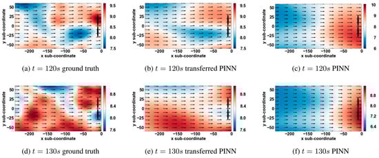
Figure 12.
Comparison of wind farms with and without PINN combined with migration learning, extracted from Chang et al. [134].
6. Opportunities and Challenges
In the building environment domain, CFD rapid prediction technology leveraging ML-based surrogate models has exhibited considerable potential. Nevertheless, for ML surrogate models to be broadly and reliably integrated into engineering practice, several critical challenges must still be overcome. These challenges span data availability, multi-physics coupling, and generalization capacity, each of which imposes constraints on model performance, applicability, and scalability (Figure 13).
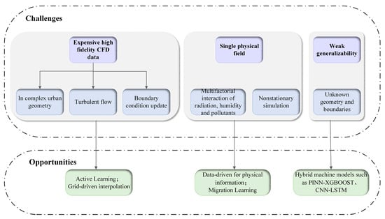
Figure 13.
Challenges and opportunities for rapid ML-based CFD prediction.
One of the primary challenges is acquiring high-quality, diverse, and physically representative datasets. Generating training datasets through high-fidelity CFD simulations incurs substantial computational costs, particularly for transient or turbulent flows in complex urban geometries. Most datasets inadequately cover the extensive parameter space encountered in real-world scenarios, which diminishes the model’s representativeness. Moreover, rapid CFD predictions necessitate dynamic updates of boundary conditions, yet existing datasets are predominantly static and struggle to capture temporal correlations. For example, in urban wind field prediction, models must capture time-varying turbulent features, while traditional data-driven methods are prone to inaccuracies due to mismatches in time steps.
The prediction of multi-physics field coupling using data-driven surrogate models remains a challenging research topic, as most ML models are trained on single physical fields or decoupled datasets. In real-world building environments, airflows are typically influenced by complex interactions, including thermal effects, radiation, humidity, buoyancy-driven convection, pollutant diffusion, and human activities. Furthermore, transient simulations involving unstable flow behaviors add to the complexity of surrogate modeling, since maintaining temporal consistency and causal dependencies is essential [74]. While RNN and temporal convolutional networks (TCNs) provide promising initial solutions, their stability, interpretability, and scalability remain constrained in large-scale, high-resolution CFD applications.
When utilizing ML-based surrogate models for CFD predictions in arbitrary building environments, the generalization capability represents a critical bottleneck during deployment. While many models demonstrate high accuracy within the distribution of training data, they struggle to extrapolate effectively when faced with unseen geometries or boundary conditions. This limitation arises partly because data-driven models are inherently inductive and lack explicit physical constraints derived from governing equations such as the Navier–Stokes equations.
Currently, active learning, physics-informed data augmentation techniques, and grid-driven interpolation strategies present key approaches to reduce the computational cost of generating high-fidelity CFD data while expanding data coverage. In handling complex coupled systems, hybrid ML models offer a scalable solution. For example, the PINN-XGBoost hybrid model exploits the physics-aware capabilities of PINN to compensate for the physical agnosticism of traditional ML models, while leveraging the ensemble learning strengths of XGBoost to manage high-dimensional nonlinear boundary conditions [141]. By incorporating physical information-based loss functions to constrain model outputs and adopting a cross-domain transfer learning framework, the model’s adaptability across different domains can be significantly enhanced. The development of lightweight surrogate models holds promise for enabling real-time digital twins in building operations, providing rapid feedback for energy optimization, ventilation control, and emergency response. This equips decision-makers with timely and accurate information, thereby improving building operational efficiency and safety while reducing operational costs.
7. Conclusions
This review aims to provide a systematic overview of recent advances in ML surrogate models for accelerating CFD simulations for rapid prediction in the built environment. The review emphasizes that ML-based surrogate models, especially neural network architectures and reduced-order models, show significant potential in reducing CFD computation time. This makes them attractive for iterative design and rapid decision-making processes in complex architectural and urban environments. A key discovery is the increasing research adoption of hybrid CFD-ML frameworks, where ML accelerates key phases of the CFD workflow. For indoor and outdoor flow field prediction, surrogate models utilizing deep learning architectures have achieved significant success in approximating complex flow behaviors under different built environment configurations. The core value of CFD-ML techniques is to enable a closed loop for rapid control and optimization of the built environment. Among them, migration learning and reinforcement learning are considered to be helpful in realizing a rapid feedback system for the built environment, and further research is recommended.
However, the trade-off between prediction speed and accuracy remains a critical issue, especially for scenarios requiring high-fidelity results. It must be recognized that ML surrogate models are not intended to replace traditional CFD but to complement it by enabling rapid prototyping and exploratory analysis. Notably, ML-based proxy models will become an indispensable tool in the next generation of sustainable and intelligent building systems.
In summary, ML-accelerated CFD predictions are evolving towards more accurate, scalable, and interpretable modeling frameworks. These developments are expected to significantly enhance early-stage and detailed design workflows for the built environment, facilitating rapid feedback, data-driven control strategies, optimization of ventilation, energy efficiency, and occupant comfort. As the field evolves, interdisciplinary collaboration between ML researchers, CFD specialists, and built environment practitioners will be critical in translating theoretical advances into practical tools for sustainable design.
Author Contributions
Methodology, Z.L., W.L., and T.Y.; investigation, R.M., Y.L., L.L., and Z.L.; resources, Z.L., M.M., and T.Y.; writing—original draft preparation, R.M., Y.L., and L.L.; writing—reviewing and editing, R.M., Y.L., and Z.L.; funding acquisition, Z.L. and T.Y. All authors have read and agreed to the published version of the manuscript.
Funding
This work was supported by National Nature Science Foundation of China (Grant No. 51878442).
Data Availability Statement
Not applicable.
Conflicts of Interest
The authors declare no conflicts of interest.
Abbreviations
The following abbreviations are used in this manuscript:
| AI | Artificial Intelligence |
| ANN | Artificial Neural Network |
| CFD | Computational Fluid Dynamics |
| CNN | Convolutional Neural Networks |
| DNS | Direct Numerical Simulation |
| GAN | Generative Adversarial networks |
| LES | Large Eddy Simulation |
| LSTM | Long Short-Term Memory |
| ML | Machine Learning |
| MLP | Multi-Layer Perceptron |
| PCA | Principal Component Analysis |
| PINN | Physical information neural network |
| POD | Proper orthogonal decomposition |
| RANS | Reynolds Average Navier–Stokes |
| RF | Random Forest |
| RL | Reinforcement learning |
| RNN | Recurrent Neural Network |
References
- Murali, D.; Suresh, M.; Martin, H.; Raman, R. Aligning Net Zero Carbon-Built Environments with Sustainable Development Goals: Topic Modelling Approach to Integrating Technologies and Policies. Build. Environ. 2025, 281, 113156. [Google Scholar] [CrossRef]
- Wei, M.; Jiang, Z.; Pandey, P.; Liu, M.; Li, R.; O’Neill, Z.; Dong, B.; Hamdy, M. Energy Resilience in the Built Environment: A Comprehensive Review of Concepts, Metrics, and Strategies. Renew. Sustain. Energy Rev. 2025, 210, 115258. [Google Scholar] [CrossRef]
- Runchal, A.K.; Rao, M.M. CFD of the Future: Year 2025 and Beyond. In 50 Years of CFD in Engineering Sciences; Springer: Singapore, 2020; pp. 779–795. [Google Scholar]
- van Leer, B.; Powell, K.G. Introduction to Computational Fluid Dynamics. In Encyclopedia of Aerospace Engineering; Wiley: New York City, NY, USA, 2010. [Google Scholar]
- Yap, J.R.; Roman, O.; Adey, B.T.; Maheshwari, T. Trends and Opportunities in Adaptive Planning for the Built Environment: A Literature Review. City Environ. Interact. 2025, 26, 100196. [Google Scholar] [CrossRef]
- Deng, X.; Nie, W.; Li, X.; Wu, J.; Yin, Z.; Han, J.; Pan, H.; Lam, C.K.C. Influence of Built Environment on Outdoor Thermal Comfort: A Comparative Study of New and Old Urban Blocks in Guangzhou. Build. Environ. 2023, 234, 110133. [Google Scholar] [CrossRef]
- Ferziger, J.H.; Perić, M.; Street, R.L. Computational Methods for Fluid Dynamics; Springer International Publishing: Cham, Germany, 2020; ISBN 978-3-319-99691-2. [Google Scholar]
- Witten, I.H.; Frank, E. Data Mining. Acm Sigmod Rec. 2002, 31, 76–77. [Google Scholar] [CrossRef]
- Bae, Y.; Nam, K.; Kang, S. CFD-ML: Stream-Based Active Learning of Computational Fluid Dynamics Simulations for Efficient Product Design. Comput. Ind. 2024, 161, 104122. [Google Scholar] [CrossRef]
- Zhu, L.-T.; Chen, X.-Z.; Ouyang, B.; Yan, W.-C.; Lei, H.; Chen, Z.; Luo, Z.-H. Review of Machine Learning for Hydrodynamics, Transport, and Reactions in Multiphase Flows and Reactors. Ind. Eng. Chem. Res. 2022, 61, 9901–9949. [Google Scholar] [CrossRef]
- Mukhamediev, R.I.; Popova, Y.; Kuchin, Y.; Zaitseva, E.; Kalimoldayev, A.; Symagulov, A.; Levashenko, V.; Abdoldina, F.; Gopejenko, V.; Yakunin, K.; et al. Review of Artificial Intelligence and Machine Learning Technologies: Classification, Restrictions, Opportunities and Challenges. Mathematics 2022, 10, 2552. [Google Scholar] [CrossRef]
- Verma, H.; Sonparote, R. Forecasting of Pressure Coefficient for Wind Interference Due to Surrounding Tall Building on a Tall Rectangular Building Using CFD Data Trained Machine Learning Models. Structures 2025, 75, 108705. [Google Scholar] [CrossRef]
- Sun, X.; Cao, W.; Shan, X.; Liu, Y.; Zhang, W. A Generalized Framework for Integrating Machine Learning into Computational Fluid Dynamics. J. Comput. Sci. 2024, 82, 102404. [Google Scholar] [CrossRef]
- Portal-Porras, K.; Fernandez-Gamiz, U.; Zulueta, E.; Irigaray, O.; Garcia-Fernandez, R. Hybrid LSTM+CNN Architecture for Unsteady Flow Prediction. Mater. Today Commun. 2023, 35, 106281. [Google Scholar] [CrossRef]
- Hu, B.; Yin, Z.; Hamrani, A.; Leon, A.; McDaniel, D. Super-Resolution-Assisted Rapid High-Fidelity CFD Modeling of Data Centers. Build. Environ. 2024, 247, 111036. [Google Scholar] [CrossRef]
- Zhou, Q.; Ooka, R. Influence of Data Preprocessing on Neural Network Performance for Reproducing CFD Simulations of Non-Isothermal Indoor Airflow Distribution. Energy Build. 2021, 230, 110525. [Google Scholar] [CrossRef]
- Yu, T.; Wu, X.; Yu, Y.; Li, R.; Zhang, H. Establishment and Validation of a Relationship Model between Nozzle Experiments and CFD Results Based on Convolutional Neural Network. Aerosp. Sci. Technol. 2023, 142, 108694. [Google Scholar] [CrossRef]
- Lang, Y.; Ng, M.X.Y.; Yu, K.X.; Chen, B.; Tan, P.C.; Tan, K.W.; Lam, W.H.; Siwayanan, P.; Kim, K.S.; Choong, T.S.Y.; et al. A Novel CFD-MILP-ANN Approach for Optimizing Sensor Placement, Number, and Source Localization in Large-Scale Gas Dispersion from Unknown Locations. Digit. Chem. Eng. 2025, 14, 100216. [Google Scholar] [CrossRef]
- Abhijeet Ganesh, G.; Lata Sinha, S.; Nath Verma, T.; Kumar Dewangan, S. Energy Consumption and Thermal Comfort Assessment Using CFD in a Naturally Ventilated Indoor Environment under Different Ventilations. Therm. Sci. Eng. Prog. 2024, 50, 102557. [Google Scholar] [CrossRef]
- Wijesooriya, K.; Mohotti, D.; Lee, C.-K.; Mendis, P. A Technical Review of Computational Fluid Dynamics (CFD) Applications on Wind Design of Tall Buildings and Structures: Past, Present and Future. J. Build. Eng. 2023, 74, 106828. [Google Scholar] [CrossRef]
- Liu, R.; Wang, Y.; Zhang, Y.; Peng, Z.; Chen, H.; Li, X.; Li, H.; Li, W. Analysis of the City-Scale Wind Environment and Detection of Ventilation Corridors in High-Density Metropolitan Areas Based on CFD Method. Urban. Clim. 2025, 59, 102274. [Google Scholar] [CrossRef]
- Blocken, B.; Stathopoulos, T.; van Beeck, J.P.A.J. Pedestrian-Level Wind Conditions around Buildings: Review of Wind-Tunnel and CFD Techniques and Their Accuracy for Wind Comfort Assessment. Build. Environ. 2016, 100, 50–81. [Google Scholar] [CrossRef]
- Blocken, B. LES over RANS in Building Simulation for Outdoor and Indoor Applications: A Foregone Conclusion? Build. Simul. 2018, 11, 821–870. [Google Scholar] [CrossRef]
- Iskandar, L.; Bay-Sahin, E.; Martinez-Molina, A.; Toker Beeson, S. Evaluation of Passive Cooling through Natural Ventilation Strategies in Historic Residential Buildings Using CFD Simulations. Energy Build. 2024, 308, 114005. [Google Scholar] [CrossRef]
- Zhao, L.; Zhou, Q.; Li, M.; Wang, Z. Evaluating Different CFD Surrogate Modelling Approaches for Fast and Accurate Indoor Environment Simulation. J. Build. Eng. 2024, 95, 110221. [Google Scholar] [CrossRef]
- Liu, H.; He, S.; Shen, L.; Hong, J. Simulation-Based Study of COVID-19 Outbreak Associated with Air-Conditioning in a Restaurant. Phys. Fluids 2021, 33, 023301. [Google Scholar] [CrossRef]
- van Hooff, T.; Blocken, B. CFD Evaluation of Natural Ventilation of Indoor Environments by the Concentration Decay Method: CO2 Gas Dispersion from a Semi-Enclosed Stadium. Build. Environ. 2013, 61, 1–17. [Google Scholar] [CrossRef]
- Gilani, S.; Montazeri, H.; Blocken, B. CFD Simulation of Stratified Indoor Environment in Displacement Ventilation: Validation and Sensitivity Analysis. Build. Environ. 2016, 95, 299–313. [Google Scholar] [CrossRef]
- Vonlanthen, M.; Allegrini, J.; Carmeliet, J. Multiscale Interaction between a Cluster of Buildings and the ABL Developing over a Real Terrain. Urban. Clim. 2017, 20, 1–19. [Google Scholar] [CrossRef]
- Robinson, D.; Brambilla, S.; Oliveto, J.; Brown, M.J.; Atchley, A.; Linn, R.R. The Effect of Terrain-Influenced Winds on Fire Spread in QUIC-Fire. Environ. Model. Softw. 2023, 167, 105727. [Google Scholar] [CrossRef]
- Yang, L.; Li, Y. City Ventilation of Hong Kong at No-Wind Conditions. Atmos. Environ. 2009, 43, 3111–3121. [Google Scholar] [CrossRef]
- Zhang, H.; Wang, L.; Yang, P.; Liu, Y.; Zhu, C.; Wang, L.; Zhong, H. Optimizing Air Inlet Designs for Enhanced Natural Ventilation in Indoor Substations: A Numerical Modelling and CFD Simulation Study. Case Stud. Therm. Eng. 2024, 59, 104408. [Google Scholar] [CrossRef]
- Islam, M.T.; Chen, Y.; Seong, D.; Verhougstraete, M.; Son, Y.-J. Effects of Recirculation and Air Change per Hour on COVID-19 Transmission in Indoor Settings: A CFD Study with Varying HVAC Parameters. Heliyon 2024, 10, e35092. [Google Scholar] [CrossRef]
- Talaat, K.; Abuhegazy, M.; Mahfoze, O.A.; Anderoglu, O.; Poroseva, S.V. Simulation of Aerosol Transmission on a Boeing 737 Airplane with Intervention Measures for COVID-19 Mitigation. Phys. Fluids 2021, 33, 033312. [Google Scholar] [CrossRef]
- Kang, Y.; Yuk, H.; Jo, H.H.; Kim, S. Indoor Thermal Environment Assessment of a Historic Building for a Thermal and Energy Retrofit Scenario Using a CFD Model. Case Stud. Therm. Eng. 2024, 63, 105330. [Google Scholar] [CrossRef]
- K, D.; Liang, H.; Lin, J.; Xie, Y.; Yu, Y.; Niu, J. Evaluating Thermal Sensation in Outdoor Environments–Different Methods of Coupling CFD and Radiation Modelling with a Human Body Thermoregulation Model. Build. Environ. 2024, 266, 112081. [Google Scholar] [CrossRef]
- Mei, S.-J.; Hang, J.; Fan, Y.; Yuan, C.; Xue, Y. CFD Simulations on the Wind and Thermal Environment in Urban Areas with Complex Terrain under Calm Conditions. Sustain. Cities Soc. 2025, 118, 106022. [Google Scholar] [CrossRef]
- Aydin, E.E.; Ortner, F.P.; Peng, S.; Yenardi, A.; Chen, Z.; Tay, J.Z. Climate-Responsive Urban Planning through Generative Models: Sensitivity Analysis of Urban Planning and Design Parameters for Urban Heat Island in Singapore’s Residential Settlements. Sustain. Cities Soc. 2024, 114, 105779. [Google Scholar] [CrossRef]
- Hang, J.; Xu, Y.; Hua, J.; Wang, W.; Zhao, B.; Zeng, L.; Du, Y. A Framework Combining Multi-Scale Model and Unmanned Aerial Vehicle for Investigating Urban Micro-Meteorology, Thermal Comfort, and Energy Balance. Sustain. Cities Soc. 2024, 115, 105847. [Google Scholar] [CrossRef]
- Rodriguez, A.; Lecigne, B.; Wood, S.; Carmeliet, J.; Kubilay, A.; Derome, D. Optimal Representation of Tree Foliage for Local Urban Climate Modeling. Sustain. Cities Soc. 2024, 115, 105857. [Google Scholar] [CrossRef]
- Zhao, R.; Liu, S.; Liu, J.; Jiang, N.; Chen, Q. A Two-Stage CFD-GNN Approach for Efficient Steady-State Prediction of Urban Airflow and Airborne Contaminant Dispersion. Sustain. Cities Soc. 2024, 112, 105607. [Google Scholar] [CrossRef]
- Blocken, B.; Stathopoulos, T. CFD Simulation of Pedestrian-Level Wind Conditions around Buildings: Past Achievements and Prospects. J. Wind. Eng. Ind. Aerodyn. 2013, 121, 138–145. [Google Scholar] [CrossRef]
- Chen, Q. Ventilation Performance Prediction for Buildings: A Method Overview and Recent Applications. Build. Environ. 2009, 44, 848–858. [Google Scholar] [CrossRef]
- Tominaga, Y.; Mochida, A.; Yoshie, R.; Kataoka, H.; Nozu, T.; Yoshikawa, M.; Shirasawa, T. AIJ Guidelines for Practical Applications of CFD to Pedestrian Wind Environment around Buildings. J. Wind Eng. Ind. Aerodyn. 2008, 96, 1749–1761. [Google Scholar] [CrossRef]
- He, G.; Yang, X.; Srebric, J. Removal of Contaminants Released from Room Surfaces by Displacement and Mixing Ventilation: Modeling and Validation. Indoor Air 2005, 15, 367–380. [Google Scholar] [CrossRef]
- Hagström, K.; Zhivov, A.M.; Sirén, K.; Christianson, L.L. Influence of the Floor-Based Obstructions on Contaminant Removal Efficiency and Effectiveness. Build. Environ. 2002, 37, 55–66. [Google Scholar] [CrossRef]
- Baitureyeva, A.; Yang, T.; Wang, H.S. Development of Machine Learning-Aided Rapid CFD Prediction for Optimal Urban Wind Environment Design. Sustain. Cities Soc. 2025, 121, 106208. [Google Scholar] [CrossRef]
- Guo, Y.; Wang, Y.; Cao, Y.; Long, Z. A New Optimization Design Method of Multi-Objective Indoor Air Supply Using the Kriging Model and NSGA-II. Appl. Sci. 2023, 13, 10465. [Google Scholar] [CrossRef]
- Wei, C.; Ooka, R. Indoor Airflow Field Reconstruction Using Physics-Informed Neural Network. Build. Environ. 2023, 242, 110563. [Google Scholar] [CrossRef]
- Liang, L.; Zhao, M.; Wang, Y.; Long, Z.; Yin, H. Optimization of Indoor Thermal Environment for High-Altitude Sentry Buildings with Attached Ventilation Based on Proper Orthogonal Decomposition. Build. Environ. 2025, 267, 112200. [Google Scholar] [CrossRef]
- Haftka, R.T.; Villanueva, D.; Chaudhuri, A. Parallel Surrogate-Assisted Global Optimization with Expensive Functions—A Survey. Struct. Multidiscip. Optim. 2016, 54, 3–13. [Google Scholar] [CrossRef]
- Jansson, T.; Nilsson, L.; Redhe, M. Using Surrogate Models and Response Surfaces in Structural Optimization ? With Application to Crashworthiness Design and Sheet Metal Forming. Struct. Multidiscip. Optim. 2003, 25, 129–140. [Google Scholar] [CrossRef]
- Tao, J.; Sun, G. Application of Deep Learning Based Multi-Fidelity Surrogate Model to Robust Aerodynamic Design Optimization. Aerosp. Sci. Technol. 2019, 92, 722–737. [Google Scholar] [CrossRef]
- Laverge, J.; Janssens, A. Optimization of Design Flow Rates and Component Sizing for Residential Ventilation. Build Environ 2013, 65, 81–89. [Google Scholar] [CrossRef]
- Li, K.; Xue, W.; Xu, C.; Su, H. Optimization of Ventilation System Operation in Office Environment Using POD Model Reduction and Genetic Algorithm. Energy Build. 2013, 67, 34–43. [Google Scholar] [CrossRef]
- Sun, T.; Feng, B.; Huo, J.; Xiao, Y.; Wang, W.; Peng, J.; Li, Z.; Du, C.; Wang, W.; Zou, G.; et al. Artificial Intelligence Meets Flexible Sensors: Emerging Smart Flexible Sensing Systems Driven by Machine Learning and Artificial Synapses. Nanomicro Lett. 2024, 16, 14. [Google Scholar] [CrossRef]
- Yaghoubi, E.; Yaghoubi, E.; Khamees, A.; Razmi, D.; Lu, T. A Systematic Review and Meta-Analysis of Machine Learning, Deep Learning, and Ensemble Learning Approaches in Predicting EV Charging Behavior. Eng. Appl. Artif. Intell. 2024, 135, 108789. [Google Scholar] [CrossRef]
- Jordan, M.I.; Mitchell, T.M. Machine Learning: Trends, Perspectives, and Prospects. Science (1979) 2015, 349, 255–260. [Google Scholar] [CrossRef]
- Caron, C.; Lauret, P.; Bastide, A. Machine Learning to Speed up Computational Fluid Dynamics Engineering Simulations for Built Environments: A Review. Build. Environ. 2025, 267, 112229. [Google Scholar] [CrossRef]
- Luo, Y.; Cui, D.; Song, Y.; Tian, Z.; Fan, J.; Zhang, L. Fast and Accurate Prediction of Air Temperature and Velocity Field in Non-Uniform Indoor Environment under Complex Boundaries. Build. Environ. 2023, 230, 109987. [Google Scholar] [CrossRef]
- Shakya, A.K.; Pillai, G.; Chakrabarty, S. Reinforcement Learning Algorithms: A Brief Survey. Expert. Syst. Appl. 2023, 231, 120495. [Google Scholar] [CrossRef]
- Du, K.; Chen, B. A Hybrid Semi-Supervised Regression Based Machine Learning Method for Predicting Peak Wind Loads on a Group of Buildings. Eng. Struct. 2023, 275, 115245. [Google Scholar] [CrossRef]
- Rumelhart, D.E.; Hinton, G.E.; Williams, R.J. Learning Representations by Back-Propagating Errors. Nature 1986, 323, 533–536. [Google Scholar] [CrossRef]
- Yao, G.; Lei, T.; Zhong, J. A Review of Convolutional-Neural-Network-Based Action Recognition. Pattern Recognit. Lett. 2019, 118, 14–22. [Google Scholar] [CrossRef]
- Jin, X.; Cheng, P.; Chen, W.-L.; Li, H. Prediction Model of Velocity Field around Circular Cylinder over Various Reynolds Numbers by Fusion Convolutional Neural Networks Based on Pressure on the Cylinder. Phys. Fluids 2018, 30, 047105. [Google Scholar] [CrossRef]
- Zhu, J.; Jiang, Q.; Shen, Y.; Qian, C.; Xu, F.; Zhu, Q. Application of Recurrent Neural Network to Mechanical Fault Diagnosis: A Review. J. Mech. Sci. Technol. 2022, 36, 527–542. [Google Scholar] [CrossRef]
- Lee, Y.; Lee, S. A Prediction of Urban Boundary Layer Using Recurrent Neural Network and Reduced Order Modeling. Build. Environ. 2025, 276, 112804. [Google Scholar] [CrossRef]
- Xie, H.-R.; Hua, Y.; Li, Y.-B.; Aubry, N.; Wu, W.-T.; He, Y.; Peng, J.-Z. Estimation of Sequential Transient Flow around Cylinders Using Recurrent Neural Network Coupled Graph Convolutional Network. Ocean. Eng. 2024, 293, 116684. [Google Scholar] [CrossRef]
- Smagulova, K.; James, A.P. A Survey on LSTM Memristive Neural Network Architectures and Applications. Eur. Phys. J. Spec. Top. 2019, 228, 2313–2324. [Google Scholar] [CrossRef]
- Raissi, M.; Perdikaris, P.; Karniadakis, G.E. Physics-Informed Neural Networks: A Deep Learning Framework for Solving Forward and Inverse Problems Involving Nonlinear Partial Differential Equations. J. Comput. Phys. 2019, 378, 686–707. [Google Scholar] [CrossRef]
- Vinuesa, R.; Brunton, S.L. Emerging Trends in Machine Learning for Computational Fluid Dynamics. Comput. Sci. Eng. 2022, 24, 33–41. [Google Scholar] [CrossRef]
- Sousa, P.; Rodrigues, C.V.; Afonso, A. Enhancing CFD Solver with Machine Learning Techniques. Comput. Methods Appl. Mech. Eng. 2024, 429, 117133. [Google Scholar] [CrossRef]
- Wu, J.-L.; Xiao, H.; Paterson, E. Physics-Informed Machine Learning Approach for Augmenting Turbulence Models: A Comprehensive Framework. Phys. Rev. Fluids 2018, 3, 074602. [Google Scholar] [CrossRef]
- Brunton, S.L.; Noack, B.R.; Koumoutsakos, P. Machine Learning for Fluid Mechanics. Annu. Rev. Fluid. Mech. 2020, 52, 477–508. [Google Scholar] [CrossRef]
- McConkey, R.; Yee, E.; Lien, F.S. Deep Structured Neural Networks for Turbulence Closure Modeling. Phys. Fluids 2022, 34, 035110. [Google Scholar] [CrossRef]
- Geneva, N.; Zabaras, N. Quantifying Model Form Uncertainty in Reynolds-Averaged Turbulence Models with Bayesian Deep Neural Networks. J. Comput. Phys. 2019, 383, 125–147. [Google Scholar] [CrossRef]
- Bre, F.; Gimenez, J.M.; Fachinotti, V.D. Prediction of Wind Pressure Coefficients on Building Surfaces Using Artificial Neural Networks. Energy Build. 2018, 158, 1429–1441. [Google Scholar] [CrossRef]
- Brenner, M.P.; Eldredge, J.D.; Freund, J.B. Perspective on Machine Learning for Advancing Fluid Mechanics. Phys. Rev. Fluids 2019, 4, 100501. [Google Scholar] [CrossRef]
- Vandewiel, M.R.; Eneyew, D.D.; Awol, A.D.; Capretz, M.A.M.; Bitsuamlak, G.T. Approximating CFD Simulations of Natural Ventilation: A Deep Surrogate Model with Spatial Attention Mechanism. J. Build. Eng. 2025, 105, 112425. [Google Scholar] [CrossRef]
- Liu, W.; He, Y.; Liu, Z. Indoor Pollution Control Based on Surrogate Model for Residential Buildings. Environ. Pollut. 2024, 346, 123638. [Google Scholar] [CrossRef]
- Manevitz, L.; Yousef, M.; Givoli, D. Finite–Element Mesh Generation Using Self–Organizing Neural Networks. Comput. Aided Civ. Infrastruct. Eng. 1997, 12, 233–250. [Google Scholar] [CrossRef]
- Bahreininejad, A.; Topping, B.H.V.; Khan, A.I. Finite Element Mesh Partitioning Using Neural Networks. Adv. Eng. Softw. 1996, 27, 103–115. [Google Scholar] [CrossRef]
- Jilani, H.; Bahreininejad, A.; Ahmadi, M.T. Adaptive Finite Element Mesh Triangulation Using Self-Organizing Neural Networks. Adv. Eng. Softw. 2009, 40, 1097–1103. [Google Scholar] [CrossRef]
- Manevitz, L.; Bitar, A.; Givoli, D. Neural Network Time Series Forecasting of Finite-Element Mesh Adaptation. Neurocomputing 2005, 63, 447–463. [Google Scholar] [CrossRef]
- Bidaguren, I.; Remaki, L.; Blanco, J.M. POD and Mesh-Adaptivity Based Reduce Order Model: Application to Solve PDEs and Inviscid Flows. Proc. Inst. Mech. Eng. G. J. Aerosp. Eng. 2025, 239, 509–527. [Google Scholar] [CrossRef]
- Zhang, X.; Xie, F.; Ji, T.; Zhu, Z.; Zheng, Y. Multi-Fidelity Deep Neural Network Surrogate Model for Aerodynamic Shape Optimization. Comput. Methods Appl. Mech. Eng. 2021, 373, 113485. [Google Scholar] [CrossRef]
- Guo, Y.; Wang, C.; Ma, Z.; Huang, X.; Sun, K.; Zhao, R. A New Mesh Smoothing Method Based on a Neural Network. Comput. Mech. 2022, 69, 425–438. [Google Scholar] [CrossRef]
- Lock, C.; Hassan, O.; Sevilla, R.; Jones, J. Meshing Using Neural Networks for Improving the Efficiency of Computer Modelling. Eng. Comput. 2023, 39, 3791–3820. [Google Scholar] [CrossRef]
- XU, R.; LYU, H.; YU, J.; BAO, C.; WANG, H.; LIU, Y.; LIU, X. Implicit Geometry Neural Network for Mesh Generation. Chin. J. Aeronaut. 2025, 38, 103315. [Google Scholar] [CrossRef]
- Peng, J.; Chen, X.; Liu, J. 3DMeshNet: A Three-Dimensional Differential Neural Network for Structured Mesh Generation. Graph. Models 2025, 139, 101257. [Google Scholar] [CrossRef]
- Vinuesa, R.; Brunton, S.L. Enhancing Computational Fluid Dynamics with Machine Learning. Nat. Comput. Sci. 2022, 2, 358–366. [Google Scholar] [CrossRef]
- Duru, C.; Alemdar, H.; Baran, Ö.U. CNNFOIL: Convolutional Encoder Decoder Modeling for Pressure Fields around Airfoils. Neural Comput. Appl. 2021, 33, 6835–6849. [Google Scholar] [CrossRef]
- Chen, D.; Gao, X.; Xu, C.; Chen, S.; Fang, J.; Wang, Z.; Wang, Z. FlowGAN: A Conditional Generative Adversarial Network for Flow Prediction in Various Conditions. In Proceedings of the 2020 IEEE 32nd International Conference on Tools with Artificial Intelligence (ICTAI), Baltimore, MD, USA, 9–11 November 2020; IEEE: Piscataway, NJ, USA, 2020; pp. 315–322. [Google Scholar]
- Yousif, M.Z.; Yu, L.; Lim, H. Physics-Guided Deep Learning for Generating Turbulent Inflow Conditions. J. Fluid. Mech. 2022, 936, A21. [Google Scholar] [CrossRef]
- Ling, J.; Kurzawski, A.; Templeton, J. Reynolds Averaged Turbulence Modelling Using Deep Neural Networks with Embedded Invariance. J. Fluid. Mech. 2016, 807, 155–166. [Google Scholar] [CrossRef]
- Majchrzak, M.; Marciniak-Lukasiak, K.; Lukasiak, P. A Survey on the Application of Machine Learning in Turbulent Flow Simulations. Energies 2023, 16, 1755. [Google Scholar] [CrossRef]
- Kochkov, D.; Smith, J.A.; Alieva, A.; Wang, Q.; Brenner, M.P.; Hoyer, S. Machine Learning–Accelerated Computational Fluid Dynamics. Proc. Natl. Acad. Sci. USA 2021, 118, e2101784118. [Google Scholar] [CrossRef] [PubMed]
- Zhang, Z.; Song, X.; Ye, S.; Wang, Y.; Huang, C.; An, Y.; Chen, Y. Application of Deep Learning Method to Reynolds Stress Models of Channel Flow Based on Reduced-Order Modeling of DNS Data. J. Hydrodyn. 2019, 31, 58–65. [Google Scholar] [CrossRef]
- Calzolari, G.; Liu, W. Deep Learning to Develop Zero-Equation Based Turbulence Model for CFD Simulations of the Built Environment. Build. Simul. 2024, 17, 399–414. [Google Scholar] [CrossRef]
- Sousa, P.; Afonso, A.; Veiga Rodrigues, C. Application of Machine Learning to Model the Pressure Poisson Equation for Fluid Flow on Generic Geometries. Neural Comput. Appl. 2024, 36, 16581–16606. [Google Scholar] [CrossRef]
- Vincent, P.; Larochelle, H.; Bengio, Y.; Manzagol, P.-A. Extracting and Composing Robust Features with Denoising Autoencoders. In Proceedings of the 25th International Conference on Machine Learning—ICML ’08, Helsinki, Finland, 5–9 July 2008; ACM Press: New York, NY, USA, 2008; pp. 1096–1103. [Google Scholar]
- Dai, Y.; Zhao, J.; Zhang, X.; Bai, F.; Tao, W.; Wang, Y. Thermal Full-Field Prediction of an Air-Cooled Data Center Using a Novel Multi-Scale Approach Based on POD and CFD Coupling. Energy Build. 2024, 307, 113992. [Google Scholar] [CrossRef]
- Min, G.; Jiang, N. Flow Fields Prediction for Data-Driven Model of Parallel Twin Cylinders Based on POD-RBFNN and POD-BPNN Surrogate Models. Ann. Nucl. Energy 2024, 199, 110342. [Google Scholar] [CrossRef]
- Deng, Z.; He, C.; Liu, Y.; Kim, K.C. Data-Driven, Physics-Based Feature Extraction from Fluid Flow Fields. Commun. Comput. Phys. 2019, 25, 625–650. [Google Scholar] [CrossRef]
- Buzzicotti, M. Data Reconstruction for Complex Flows Using AI: Recent Progress, Obstacles, and Perspectives. Europhys. Lett. 2023, 142, 23001. [Google Scholar] [CrossRef]
- Pullan, G.; Chuan, T.; Wong, D.; Jasik, F. Enhancing Web-Based CFD Post-Processing Using Machine Learning and Augmented Reality. In Proceedings of the AIAA Scitech 2019 Forum, San Diego, CA, USA, 7–11 January 2019; American Institute of Aeronautics and Astronautics: Reston, VA, USA, 2019. [Google Scholar]
- Lguensat, R.; Sun, M.; Fablet, R.; Tandeo, P.; Mason, E.; Chen, G. EddyNet: A Deep Neural Network For Pixel-Wise Classification of Oceanic Eddies. In Proceedings of the IGARSS 2018—2018 IEEE International Geoscience and Remote Sensing Symposium, Valencia, Spain, 22–27 July 2018; IEEE: Piscataway, NJ, USA, 2018; pp. 1764–1767. [Google Scholar]
- Morozova, N.; Trias, F.X.; Capdevila, R.; Schillaci, E.; Oliva, A. A CFD-Based Surrogate Model for Predicting Flow Parameters in a Ventilated Room Using Sensor Readings. Energy Build. 2022, 266, 112146. [Google Scholar] [CrossRef]
- Kashir, B.; Ragone, M.; Ramasubramanian, A.; Yurkiv, V.; Mashayek, F. Application of Fully Convolutional Neural Networks for Feature Extraction in Fluid Flow. J. Vis. (Tokyo) 2021, 24, 771–785. [Google Scholar] [CrossRef]
- Meyer, R.D.; Tan, G. Provide Detailed and Real-Time Indoor Environmental Information Using POD–LSE and Limited Measurements. Energy Build. 2014, 73, 59–68. [Google Scholar] [CrossRef]
- Sun, H.; Burton, H.V.; Huang, H. Machine Learning Applications for Building Structural Design and Performance Assessment: State-of-the-Art Review. J. Build. Eng. 2021, 33, 101816. [Google Scholar] [CrossRef]
- Zhou, Q.; Ooka, R. Comparison of Different Deep Neural Network Architectures for Isothermal Indoor Airflow Prediction. Build. Simul. 2020, 13, 1409–1423. [Google Scholar] [CrossRef]
- Hu, C.; Jia, H.; Kikumoto, H. Estimation of Airflow Distribution in Cubic Building Group Model Using POD-LSE and Limited Sensors. Build. Environ. 2022, 221, 109324. [Google Scholar] [CrossRef]
- Taira, K.; Hemati, M.S.; Brunton, S.L.; Sun, Y.; Duraisamy, K.; Bagheri, S.; Dawson, S.T.M.; Yeh, C.-A. Modal Analysis of Fluid Flows: Applications and Outlook. AIAA J. 2020, 58, 998–1022. [Google Scholar] [CrossRef]
- Taira, K.; Brunton, S.L.; Dawson, S.T.M.; Rowley, C.W.; Colonius, T.; McKeon, B.J.; Schmidt, O.T.; Gordeyev, S.; Theofilis, V.; Ukeiley, L.S. Modal Analysis of Fluid Flows: An Overview. AIAA J. 2017, 55, 4013–4041. [Google Scholar] [CrossRef]
- Pla, F.; Herrero, H.; Vega, J.M. A Flexible Symmetry-Preserving Galerkin/POD Reduced Order Model Applied to a Convective Instability Problem. Comput. Fluids 2015, 119, 162–175. [Google Scholar] [CrossRef]
- Tang, Y.-Q.; Fang, W.-Z.; Zheng, C.-Y.; Tao, W.-Q. Applications of POD-Based Reduced Order Model to the Rapid Prediction of Velocity and Temperature in Data Centers. Appl. Therm. Eng. 2025, 263, 125310. [Google Scholar] [CrossRef]
- Wang, X.; Li, D.; Zhao, J.; Cao, Z.; Weng, W. Indoor Environment Reconstruction Algorithm Based on Gappy POD and Finite Sensors. Energy Build. 2023, 297, 113463. [Google Scholar] [CrossRef]
- Calzolari, G.; Liu, W. Deep Learning to Replace, Improve, or Aid CFD Analysis in Built Environment Applications: A Review. Build. Environ. 2021, 206, 108315. [Google Scholar] [CrossRef]
- Warey, A.; Kaushik, S.; Khalighi, B.; Cruse, M.; Venkatesan, G. Data-Driven Prediction of Vehicle Cabin Thermal Comfort: Using Machine Learning and High-Fidelity Simulation Results. Int. J. Heat. Mass Transf. 2020, 148, 119083. [Google Scholar] [CrossRef]
- Wehrle, J.; Jung, C.; Giometto, M.; Christen, A.; Schindler, D. Introducing New Morphometric Parameters to Improve Urban Canopy Air Flow Modeling: A CFD to Machine-Learning Study in Real Urban Environments. Urban Clim. 2024, 58, 102173. [Google Scholar] [CrossRef]
- Lin, X.; Fu, Y.; Peng, D.Z.; Liu, C.-H.; Chu, M.; Chen, Z.; Yang, F.; Tse, T.K.T.; Li, C.Y.; Feng, X. CFD- and BPNN- Based Investigation and Prediction of Air Pollutant Dispersion in Urban Environment. Sustain. Cities Soc. 2024, 100, 105029. [Google Scholar] [CrossRef]
- Wang, T.; Li, X.; Lu, Y.; Dong, L.; Shi, F.; Lin, Z. An Efficient Thermal Comfort Prediction Method for Indoor Airflow Environment Using a CFD-Based Deep Learning Model. Build. Environ. 2025, 267, 112246. [Google Scholar] [CrossRef]
- Tian, X.; Zhang, Y.; Lin, Z. Predicting Non-Uniform Indoor Air Quality Distribution by Using Pulsating Air Supply and SVM Model. Build. Environ. 2022, 219, 109171. [Google Scholar] [CrossRef]
- Tian, X.; Cheng, Y.; Lin, Z. Modelling Indoor Environment Indicators Using Artificial Neural Network in the Stratified Environments. Build. Environ. 2022, 208, 108581. [Google Scholar] [CrossRef]
- Xu, S.; Sun, Z.; Huang, R.; Guo, D.; Yang, G.; Ju, S. A Practical Approach to Flow Field Reconstruction with Sparse or Incomplete Data through Physics Informed Neural Network. Acta Mech. Sin. 2023, 39, 322302. [Google Scholar] [CrossRef]
- Kaloop, M.R.; Bardhan, A.; Samui, P.; Hu, J.W.; Elsharawy, M. Comparative Study on Deep and Machine Learning Approaches for Predicting Wind Pressures on Tall Buildings. Alex. Eng. J. 2025, 111, 610–627. [Google Scholar] [CrossRef]
- Shao, X.; Liu, Z.; Zhang, S.; Zhao, Z.; Hu, C. PIGNN-CFD: A Physics-Informed Graph Neural Network for Rapid Predicting Urban Wind Field Defined on Unstructured Mesh. Build. Environ. 2023, 232, 110056. [Google Scholar] [CrossRef]
- Zhang, B.; Rong, Y.; Yong, R.; Qin, D.; Li, M.; Zou, G.; Pan, J. Deep Learning for Air Pollutant Concentration Prediction: A Review. Atmos. Environ. 2022, 290, 119347. [Google Scholar] [CrossRef]
- Zhou, Y.; An, Y.; Huang, W.; Chen, C.; You, R. A Combined Deep Learning and Physical Modelling Method for Estimating Air Pollutants’ Source Location and Emission Profile in Street Canyons. Build. Environ. 2022, 219, 109246. [Google Scholar] [CrossRef]
- Mendil, M.; Leirens, S.; Armand, P.; Duchenne, C. Hazardous Atmospheric Dispersion in Urban Areas: A Deep Learning Approach for Emergency Pollution Forecast. Environ. Model Softw. 2022, 152, 105387. [Google Scholar] [CrossRef]
- Huang, C.; Hu, T.; Duan, Y.; Li, Q.; Chen, N.; Wang, Q.; Zhou, M.; Rao, P. Effect of Urban Morphology on Air Pollution Distribution in High-Density Urban Blocks Based on Mobile Monitoring and Machine Learning. Build. Environ. 2022, 219, 109173. [Google Scholar] [CrossRef]
- Berenjkoub, M.; Chen, G.; Gunther, T. Vortex Boundary Identification Using Convolutional Neural Network. In Proceedings of the 2020 IEEE Visualization Conference (VIS), Salt Lake City, UT, USA, 25–30 October 2020; IEEE: Piscataway, NJ, USA, 2020; pp. 261–265. [Google Scholar]
- Yan, C.; Xu, S.; Sun, Z.; Lutz, T.; Guo, D.; Yang, G. A Framework of Data Assimilation for Wind Flow Fields by Physics-Informed Neural Networks. Appl. Energy 2024, 371, 123719. [Google Scholar] [CrossRef]
- Chaudhary, G.; Johra, H.; Georges, L.; Austbø, B. Transfer Learning in Building Dynamics Prediction. Energy Build. 2025, 330, 115384. [Google Scholar] [CrossRef]
- Park, J.; Kim, T.; Kim, D.; Alghimlas, F.; AlRagom, F.; Choi, H.; Cho, H. Field Test of Machine-Learning Based Mean Radiant Temperature Estimation Methods for Thermal Comfort-Integrated Air-Conditioning Control Improvement and Energy Savings. Energy Rep. 2024, 11, 5682–5702. [Google Scholar] [CrossRef]
- Chen, Y.; Tong, Z.; Zheng, Y.; Samuelson, H.; Norford, L. Transfer Learning with Deep Neural Networks for Model Predictive Control of HVAC and Natural Ventilation in Smart Buildings. J. Clean. Prod. 2020, 254, 119866. [Google Scholar] [CrossRef]
- Chen, Y.; Norford, L.K.; Samuelson, H.W.; Malkawi, A. Optimal Control of HVAC and Window Systems for Natural Ventilation through Reinforcement Learning. Energy Build. 2018, 169, 195–205. [Google Scholar] [CrossRef]
- Fang, Q.; Li, Z.; Wang, Y.; Song, M.; Wang, J. A Neural-Network Enhanced Modeling Method for Real-Time Evaluation of the Temperature Distribution in a Data Center. Neural Comput. Appl. 2019, 31, 8379–8391. [Google Scholar] [CrossRef]
- Zhang, J.; Zhao, X. Spatiotemporal Wind Field Prediction Based on Physics-Informed Deep Learning and LIDAR Measurements. Appl. Energy 2021, 288, 116641. [Google Scholar] [CrossRef]
- Li, X.; Sun, W.; Qin, C.; Yan, Y.; Zhang, L.; Tu, J. Evaluation of Supervised Machine Learning Regression Models for CFD-Based Surrogate Modelling in Indoor Airflow Field Reconstruction. Build Environ. 2025, 267, 112173. [Google Scholar] [CrossRef]
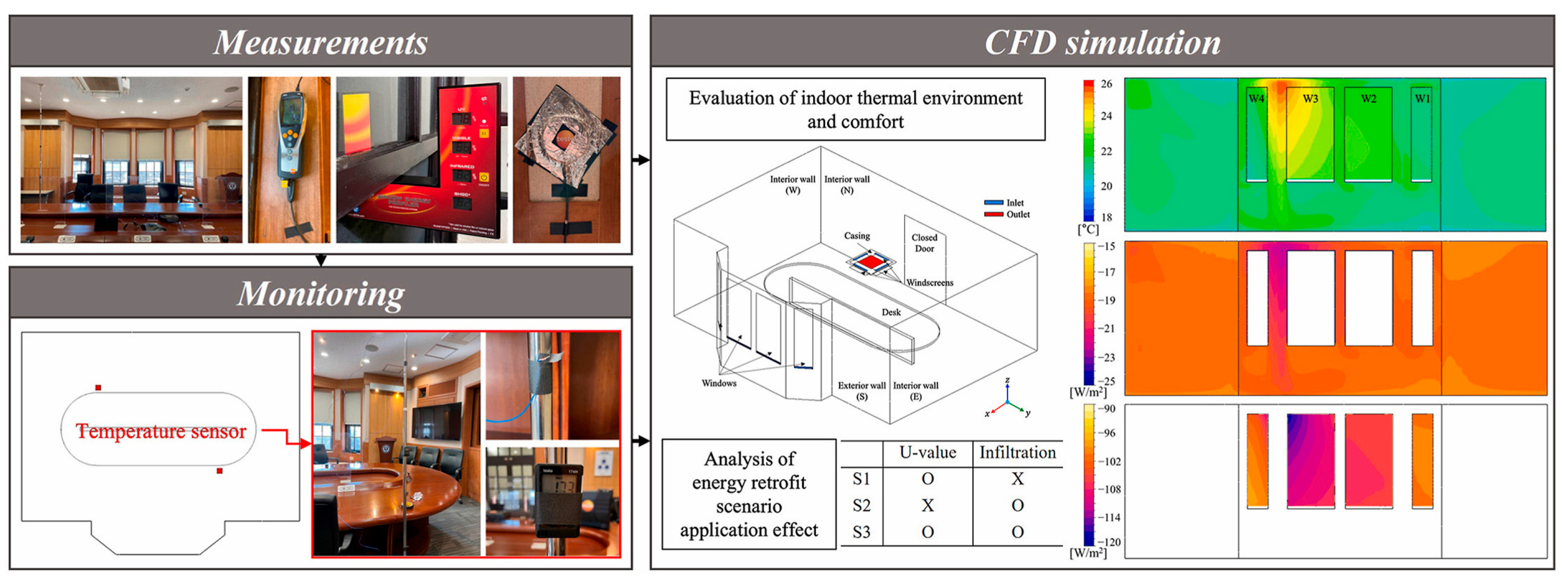
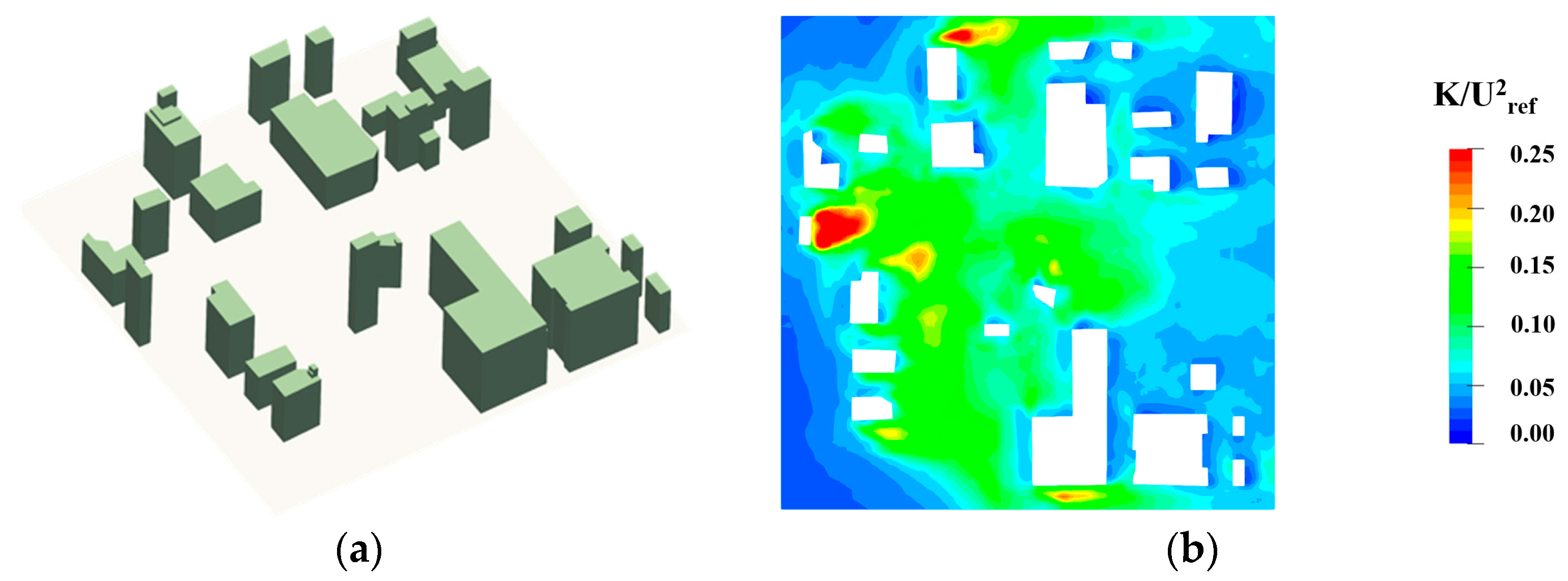
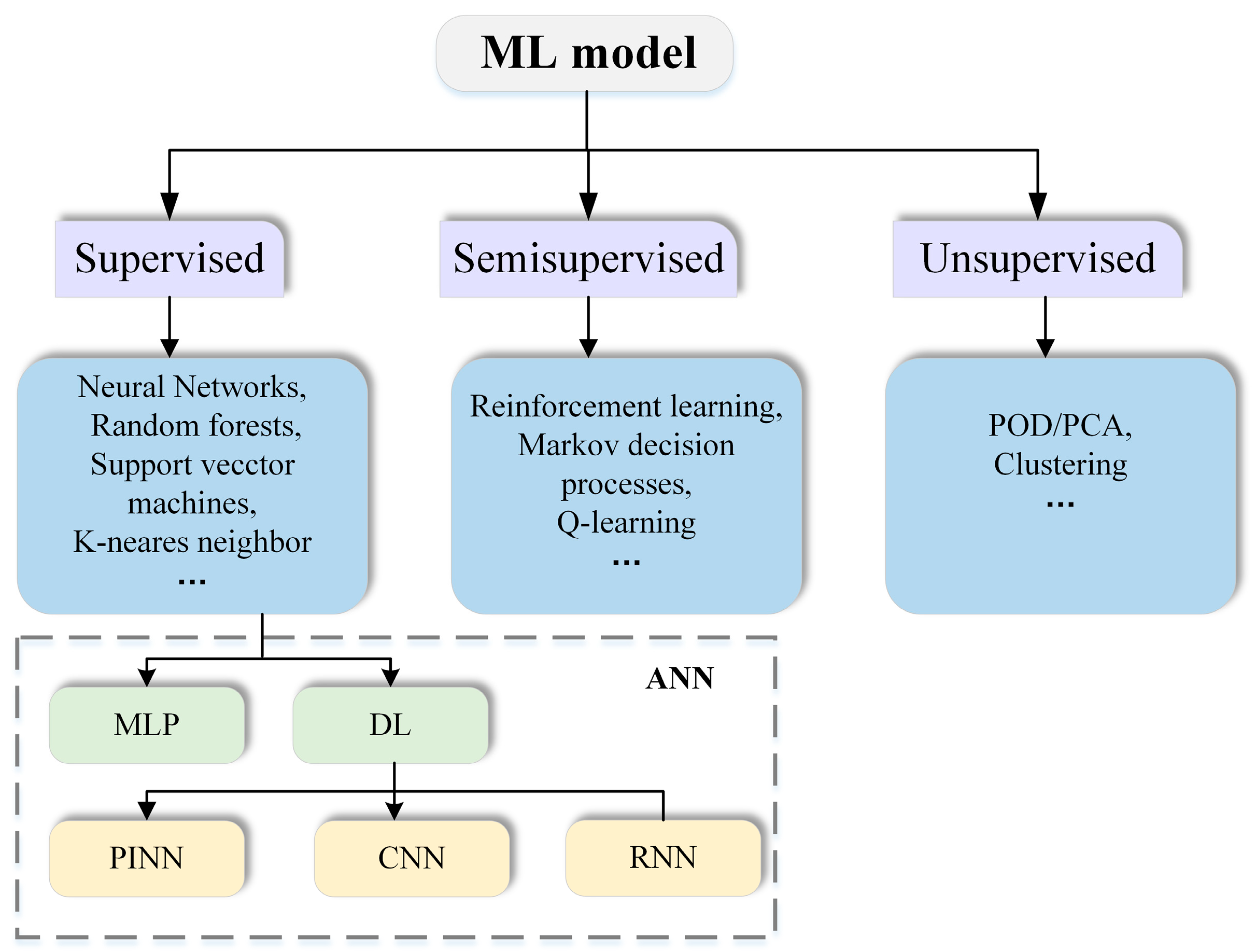
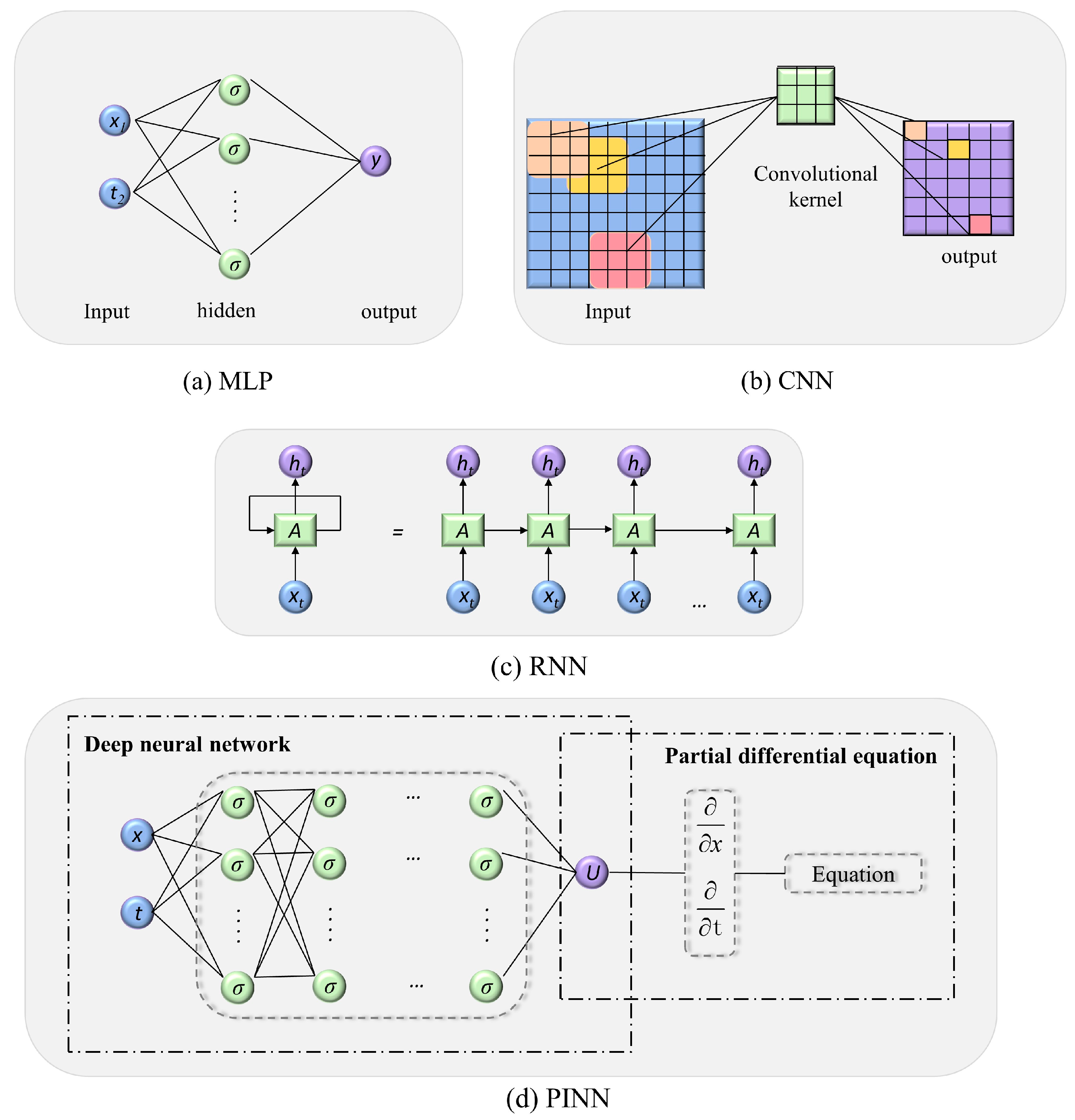
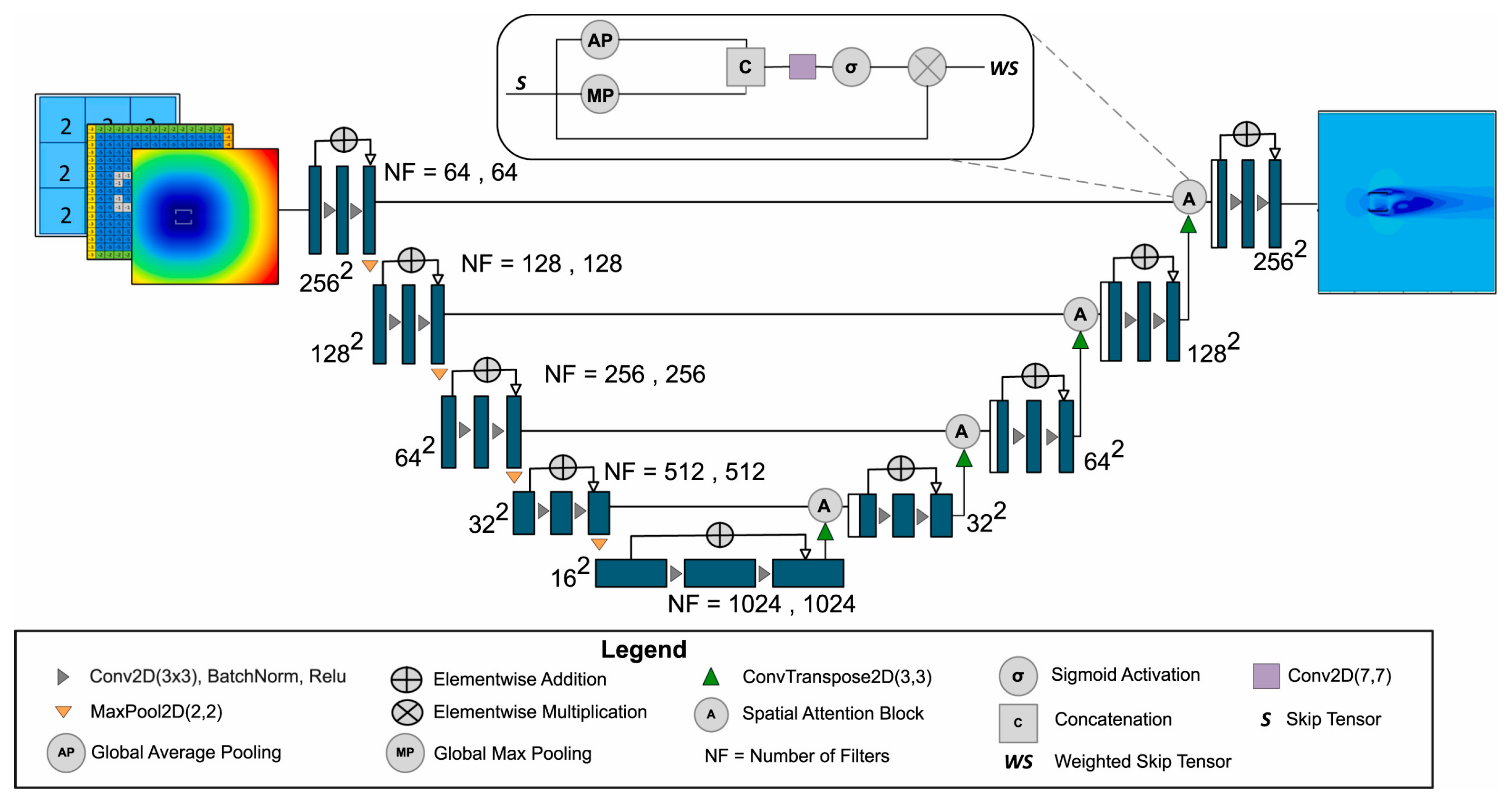


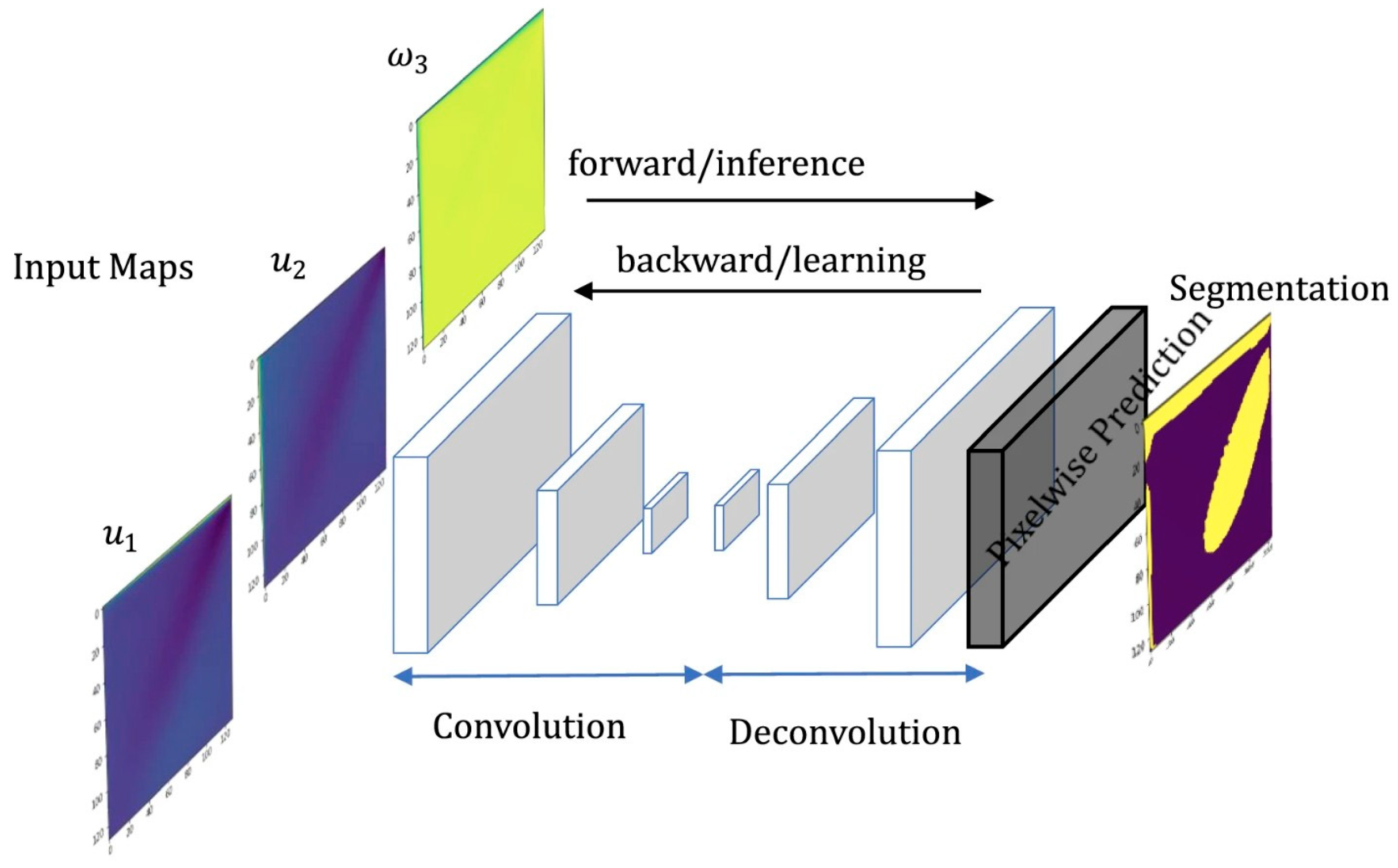

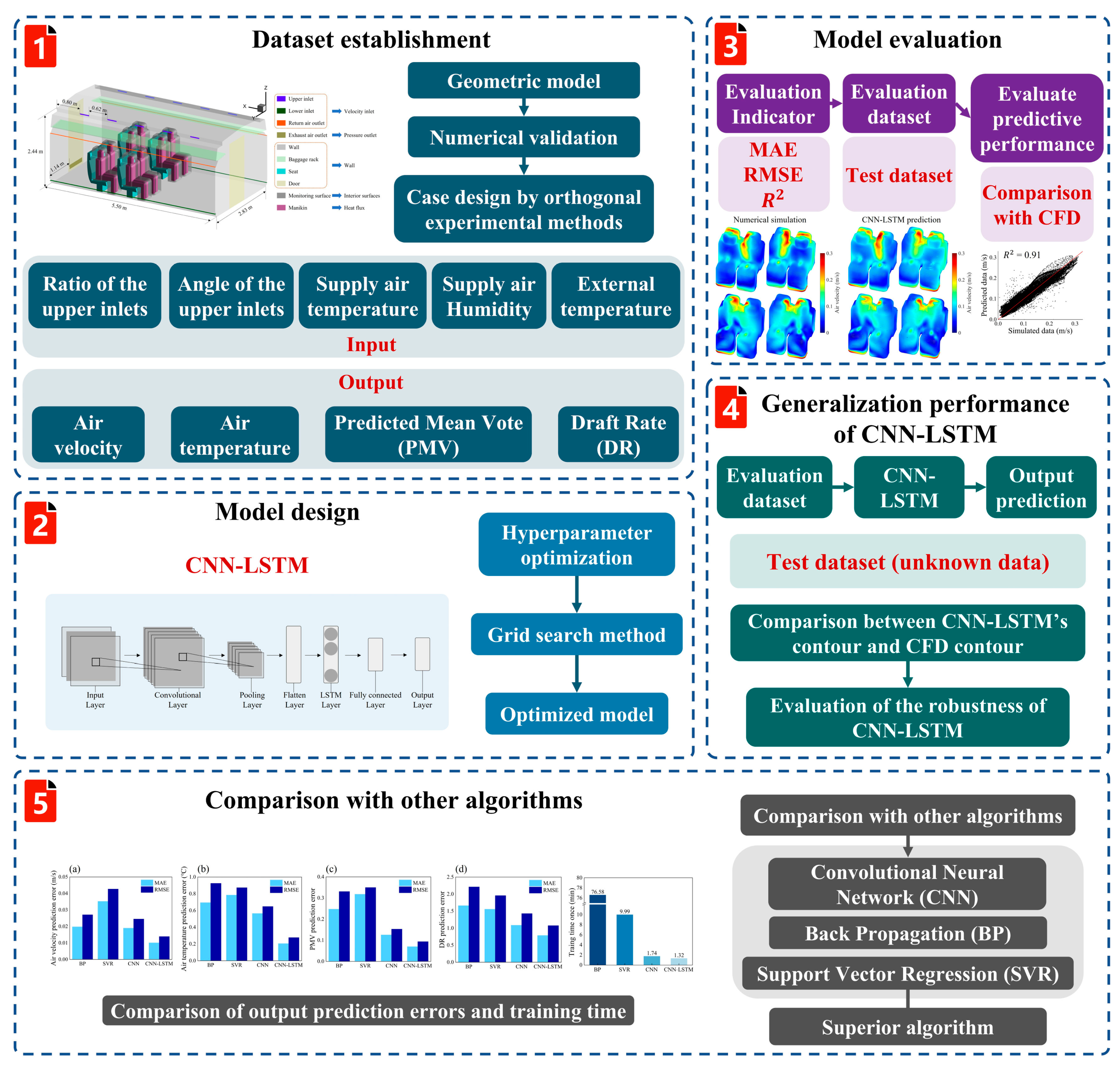


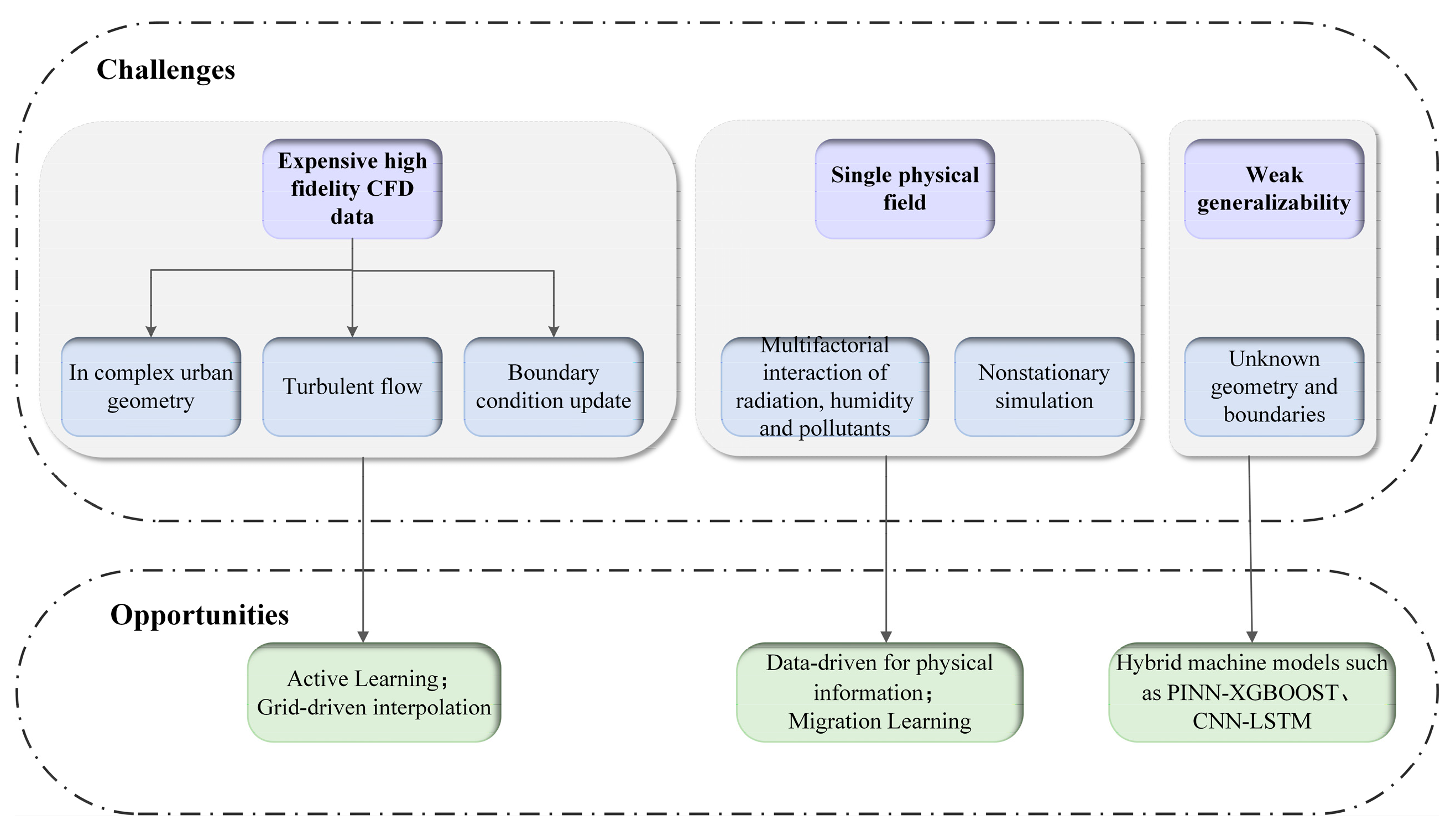
Disclaimer/Publisher’s Note: The statements, opinions and data contained in all publications are solely those of the individual author(s) and contributor(s) and not of MDPI and/or the editor(s). MDPI and/or the editor(s) disclaim responsibility for any injury to people or property resulting from any ideas, methods, instructions or products referred to in the content. |
© 2025 by the authors. Licensee MDPI, Basel, Switzerland. This article is an open access article distributed under the terms and conditions of the Creative Commons Attribution (CC BY) license (https://creativecommons.org/licenses/by/4.0/).