Abstract
Results are reported for a series of small-scale experiments that examine the dispersion of dense gas released upstream of an isolated building. The experiments replicate the geometry of the Thorney Island Phase II field tests and show good qualitative agreement with the flow regimes observed therein. The experiments were run in a water flume, and the flow is characterized by the Richardson number (), where high represent relatively high density releases. For low the dense cloud flows over and around the building and any fluid drawn into the building wake is rapidly flushed. However, for high Ri, the dense cloud collapses, flows around the building, and is drawn into the wake. The dense fluid layer becomes trapped in the wake and is flushed by small parcels of fluid being peeled off the top of the layer and driven up and out of the wake. Results are presented for the concentration field along the center plane (parallel to the flow) of the building wake and time series of concentration just above the floor and downstream of the building. The time series for low- and high- flows are starkly different, with differences explained in terms of the observed flow regimes.
1. Introduction
The world is becoming increasingly urbanized. Over half the world′s population lives in urban areas, and the urban population is expected to exceed 5 billion by 2030 [1]. High population density and increased industrialization lead to greater risk from industrial pollutants [2]. Of particular concern is the release of dense gases that can become trapped near ground level by their weight and have reduced dispersion due to trapping in the urban canopy [3,4]. Accidental releases of dense gases such as chlorine [4] and methyl isocyanate [5] can lead to serious health problems and deaths. Accidental releases of, for example, chlorine, are not uncommon. A release in a port in Jordan killed 13 people in 2022 [6]. There have also been several such releases in the USA in recent years [7,8,9]. See Ref. [10] for a discussion of the health consequences of these and other releases.
Given the risks to the life and health of urban populations, it is important to accurately model the spread and dispersion of dense gases in complex urban topography. Urban dispersion models, including those focused on dense gas dispersion, often use the so-called flat earth approximation [11]. In this assumption the details of the urban topography are treated as surface roughness that produces a drag on the spread of pollutants [12,13,14]. Therefore, the details of the flow around and between buildings are not resolved in these models. However, these flow paths can be important. It is well known that the layout of buildings in an urban area has a significant impact on the pedestrian-level winds (PLW) [15,16,17,18] and that urban canopies can have regions of very high and very low PLW. In regions of very low winds, dense gas releases can become trapped and have very high retention times and low dispersion.
Modeling of flow and dispersion in urban areas is challenging due to the complexity of urban topography and the large variety of urban layouts. Many model studies focus on simple gridded arrays of buildings and other idealizations of urban canopies [19,20,21]. However, real urban canopies are more complex and variable. For example, urban canopies have large variations in street orientation entropy [22], flow path tortuosity [23], and fractal dimension [24,25]. Therefore, it is unlikely that a generalized dense gas dispersion model will be able to resolve local flow behavior using parameterizations of urban topography given its complexity, variability, and heterogeneity. Instead, the most promising solution is to apply computational fluid dynamics (CFD) models to the problem of dense gas dispersion in urban areas [26]. Specifically, LES models [19] can model the time-varying flow through complex topography [27,28]. CFD-LES models have modeled a variety of applications, including urban mixing [19], wind loads on structures [29], and building ventilation [28]. However, the challenge with such models is the need for field data or experimental data for model validation. This validation data can range from small-scale laboratory data [30,31,32] to large-scale field experiments. The pros and cons of field and laboratory studies are described below.
Field experiments typically involve releasing large volumes of dense gas, such as chlorine, in a large open space with various obstacles located downwind of the release. The goal is to measure the downwind concentration near the various obstacles. Examples include Thorney Island [33], Jack Rabbit I [34], and Jack Rabbit II [35]. The primary advantage of field studies is that the results do not need to be adjusted for scale effects as they are run at full scale. The main disadvantages are the large cost, the limited control of the environmental conditions, and the limited spatial resolution of the measurements.
The Thorney Island dense gas dispersion experiments [36,37,38] looked at dense gas dispersion for a range of topography, including fences, a cuboid building upwind of the release point, and a cuboid building downwind of the release. The dense gas concentration was then measured at several points over time. For example, point measurements were made on the upwind and downwind faces of the cuboid building for an upwind release at a frequency of around one measurement every 8–10 s [39]. The concentration on both sides of the building showed a rapid rise followed by a slow decay. The peak concentration was higher on the upwind side of the building while the decay rate was much slower on the downwind side. This indicates that some of the dense gas became trapped in the wake of the building. The Thorney Island experiments have been reproduced in wind tunnel studies [40] and used for computational model development [39,41,42].
The Jack Rabbit I [34] and II [35] experimental campaigns used large volumes of chlorine as the dense gas. In Phase I the chlorine was released into a large circular depression in the ground. Concentrations were measured over time as the ambient wind flushed the chlorine out of the depression. Phase II focused on urban dispersion. Model urban areas were built using Conex shipping containers as buildings. Point measurements of dense gas concentration were made at a broad range of locations within the building array and at different heights. Meteorologic [43] and source condition [44] data, combined with the downwind concentration measurements, have been used for dense gas dispersion model development and validation [45,46] and to replicate the field study at the wind tunnel scale [47].
In comparison to the Thorney Island tests, Jack Rabbit had an order of magnitude more sensors, though this still only represented a handful of sensors per building. Given the highly turbulent nature of complex urban canopy flows, the concentration field will likely be heterogeneous and contain regions of high spatial gradients that may not be captured with point measurements at the spatial resolution of field studies, even for highly instrumented studies like Jack Rabbit II. Therefore, although the data is valuable and provides great insight into dense gas dispersion in urban areas, higher spatial resolution data is still needed to fully validate computational models for these types of flow.
Laboratory experiments have the advantage of having much more control of over source and ambient conditions. The use of optical measurement techniques such as dye attenuation [48] and light-induced fluorescence (LIF) [49] can significantly improve spatial resolution of measurements compared to point sensors. Laboratory experiments also have the advantage of being much less expensive, allowing a larger exploration of the parameter space. There are a large number of studies of dense gas dispersion from trapping topographies. For example, the flushing of salt water from a cavity in a riverbed has used small-scale experiments [50,51,52] that have been used to validate computational models [53]. Flushing of dense pollutants from urban canyons was studied using water channel experiments [54,55] for a broad range of canyon aspect ratios. In these experiments the density of the pollutant was parameterized in terms of a Richardson number given by
where is the height of the buildings that form the canyon, is the reduced gravity of the dense fluid, is gravitational acceleration, is the ambient fluid density, and is the reference flow veolcity. Higher Richardson numbers represent more stable flows with longer retention times for the trapped dense fluid. These experiments were run with salt as the dense pollutant and fresh water as the ambient fluid. Light attenuation measurements [48] were used to capture the concentration of dense fluid across the entire two-dimensional urban canyon at high temporal resolution. These measurements not only provided quantitative data but also detailed flow visualization that provided insight into the various mixing processes [31].
One limitation of the light attenuation measurement technique is that it provides a depth-averaged light attenuation measurement and, therefore, is only useful for two-dimensional flows. However, light-induced fluorescence (LIF) [49] allows experiments to be run in three-dimensional flows while looking at the concentration field in a two-dimensional slice through the flow. This allows the measurement of more complex flows, though the complexity is limited by the ability of a camera to view the light sheet. For example, the flow resulting from flushing dense fluid from a cavity was studied using LIF by [32].
Of particular interest to this present study was an investigation of the trapping of dense fluid in the wake of a cubic building from the continuous release of dense fluid upstream of the building [30]. LIF measurements were made in a square window that was parallel to the flow aligned with the centerline of the model building. Concentration measurements were reported for a broad range of source Richardson numbers and source flow rates. The basic geometry of the flow was similar to the Thorney Island experiments, namely a dense gas release upstream of a cubic building, with two significant differences. First, the dense fluid source was closer to the building in [30] than at Thorney Island due to the physical constraints of the experimental apparatus. Second, the source of dense fluid in [30] was continuous, whereas Thorney Island only considered finite instantaneous releases. However, the experiments of [30] did provide significant insight into the trapping of dense fluid in a building wake. For small Richardson numbers (), where there is a relatively small density difference between the pollutant and the ambient fluid densities, the wake was relatively uniformly mixed, and the pollutant concentration in the wake was very low. For higher the dense fluid became trapped at ground level and was flushed from the wake by being skimmed off the top of the dense lower layer, pushed upwind toward the building, and then up the leeward wall and out of the wake.
As the dense pollutant release was continuous, the resulting wake concentration was quasi-steady, allowing the calculation of time-averaged concentrations. Data was presented for mean concentrations at a location just above the ground and just downstream of the leeward wall. The data showed that the mean concentration at this location had a maximum value at an intermediate value of . Results were also reported for the standard deviation in the concentrations which showed qualitatively similar behavior.
While [30] provided significant qualitative and quantitative insight into the behavior of a dense pollutant trapped in the wake of a building, the study is limited by the use of a continuous source of pollutant, whereas most field studies employ finite instantaneous releases of dense gas. Furthermore, many accidental releases, such as the rupture of a chlorine tank after a train derailment [4,26], occur over relatively short periods of time compared to the time taken to disperse. Therefore, it is important to quantify both the peak concentration and decay rate from a finite release of dense pollutant.
The goal of this study is to measure the time-varying concentration of dense pollutants in the wake of a cubic building following the instantaneous release of a finite volume of pollutant. This experimental study uses the same experimental setup as [30] but focuses on finite volume releases, not continuous releases. This is directly analogous to the Thorney Island dense gas dispersion experiments [36,37,38] run at a scale ratio of 1:90 (10 cm model building compared to 9 m full-scale building). The full-scale Reynolds numbers were of the order of while the lab-scale tests were run at which, while much lower than full-scale, is above the cut-off Reynolds number for Reynolds number independent flow.
Experimental results are reported for experiments covering 23 different Richardson numbers ranging from . Due to the highly turbulent nature of the flow, each experiment was run three times to establish the ensemble behavior. The remainder of the paper is structured as follows. The experimental method is described in Section 2, including the measurement method, calibration, and experimental procedure. The qualitative results are presented in Section 3, with quantitative results in Section 4. The results are discussed in Section 5, and conclusions are drawn in Section 6.
2. Experimental Method
2.1. Experimental Setup
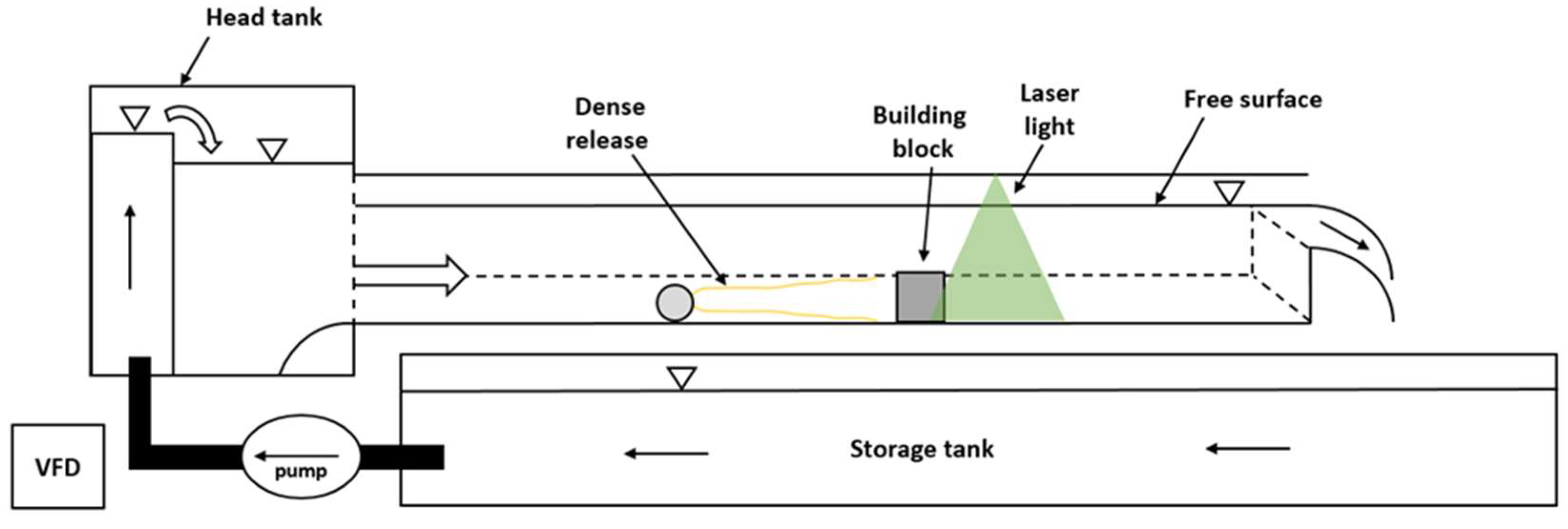
The test setup used for this study is the same as that of the study conducted in [30]. In all the experiments reported in this study, a finite volume of dyed saline water was released upstream of the building block in a free-flowing open channel filled with fresh water. This is shown schematically in Figure 1. Flow visualization was conducted using a laser light sheet on the leeward side of the building, and the results were collected there. Light-induced fluorescence (LIF) and acoustic Doppler velocimetry (ADV) techniques were used to measure the concentration of the dense fluid and velocity of the flow, respectively.
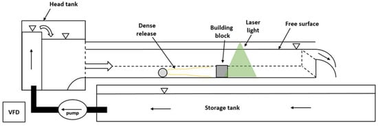
Figure 1.
Side view of the experimental setup showing the flume, model building, the finite release, and the laser light sheet. Arrows show the direction of flow.
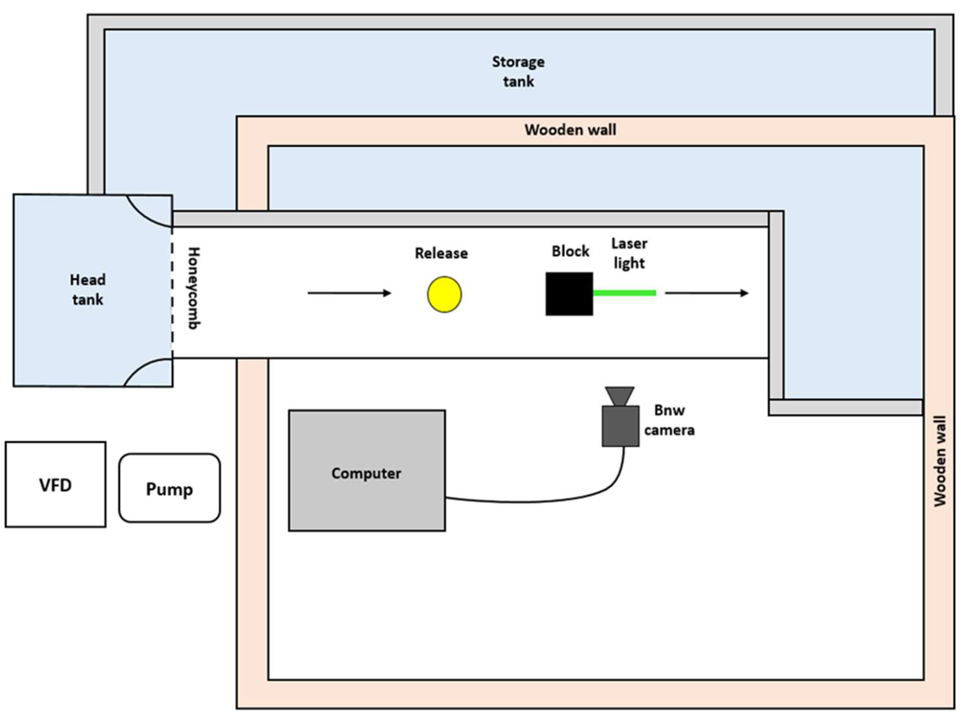
Instantaneous release experiments were conducted for a broad range of Richardson numbers at an upstream release distance of 10 cm. The instantaneous release was achieved by placing the dense fluid in a balloon and puncturing the balloon. In each experiment a balloon was connected to a quarter-turn valve, and a large syringe was used to extract all the air from the balloon. A separate syringe was then used to inject the fixed volume of dyed salt solution of known density. The volume of fluid injected was enough to stretch the balloon fabric so that it would burst when pierced. When inflated, the balloon had a diameter of approximately 8 cm. The balloon was then held in a metal ring and placed in a small metal wire basket to prevent it from moving when placed in the flowing water of the flume. The wire basket rested on the ground and had wire diameters of approximately 2 mm. While the balloon was stretched by the injection of dense salt solution, it was not rigid and was, therefore, only approximately spherical when punctured. See Figure 2 for the plan view of the experimental setup.
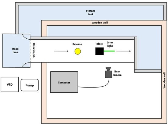
Figure 2.
Top view of the experimental setup. The upstream distance was measured from the center of the balloon to the upstream face of the model building (block). This distance was held constant at 10 cm for all the experiments reported herein. Arrows show the direction of flow.
The flowrate in the flume was controlled by a variable frequency drive connected to the pump. The depth of the flow was controlled by a sharp-crested weir at the downstream end of the flume. Upstream of the test section, the bed of the flume was covered with gravel to generate a turbulent boundary layer that was substantially taller than the model building.
2.2. Measurement Methods
The light-induced fluorescence (LIF) technique was used to measure the concentration of the fluid in the building wake. In all experiments the dense salt solution was dyed with sodium fluorescein. The fluorescence of the dye when excited by the laser sheet is linearly proportional to the product of the concentration and the laser light intensity. Light attenuation due to the dye was negligible for the concentrations used, such that the light intensity at any location was effectively constant during each experiment. The light intensity measured by the camera is due to the background light and the light due to the fluorescence of the dye. Therefore, the concentration of the (C) is given by
Here is the uniform dye concentration present in the background, is the attenuation coefficient, (x, z) is the light intensity measured by the camera, is the ambient dye light intensity of the uniform background concentration, and is the response of the camera when there is not light. The camera light response was verified to be linear [30]. It was also shown that the mean intensity of fluorescence was approximately linearly proportional to dye concentration [30]. Hence, the attenuation can be neglected. Therefore, the above equation can be written as
where is the ambient background intensity with the laser light switched off, which includes the black offset of the camera (the camera reading when no light is coming in), and is the light intensity with the laser turned on and the ambient flow running (i.e., is the light intensity measured due to the ambient concentration of dye). Before each experiment a short video was taken with all the lights off to measure , and a second video was taken to measure the light intensity due to the dye in the ambient fluid . A third video was taken in which the source solution of dyed fluid was injected directly into the laser sheet to measure the light intensity for this solution (), which is the light intensity of the fluid of the source concentration. Noting that the buoyancy of the fluid is linearly proportional to dye concentration, then the buoyancy at any location is given by
Further, the source buoyancy is given by
Such that the normalized reduced gravity can be calculated using
All results reported herein are for the normalized reduced gravity, which is the same as the concentration of the fluid normalized on the source concentration.
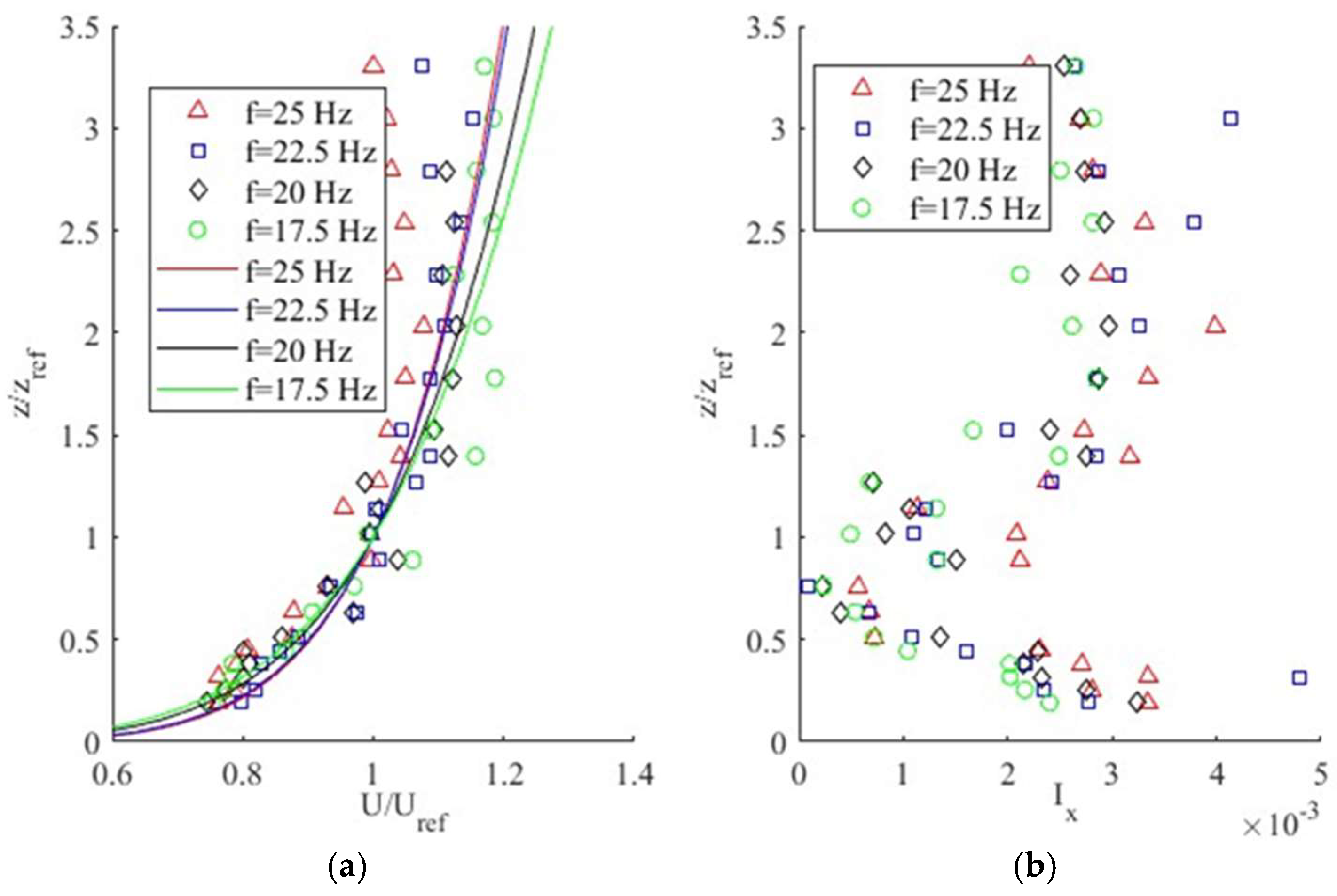
The velocity of the flow was measured using an acoustic Doppler velocimetry (ADV) probe. Boundary layer profiles were measured for four different pump frequencies. The time-averaged velocity profiles were well described as power law functions of height. The velocity measurements were made without the model building in the flume at the location where the building was placed during the experiments. The reference velocity for a given experiment was taken as the time-averaged velocity measured by the ADV at the height of the top of the building (10 cm above the flume bed). See Figure 3 for the measured velocity and turbulence intensity profiles.
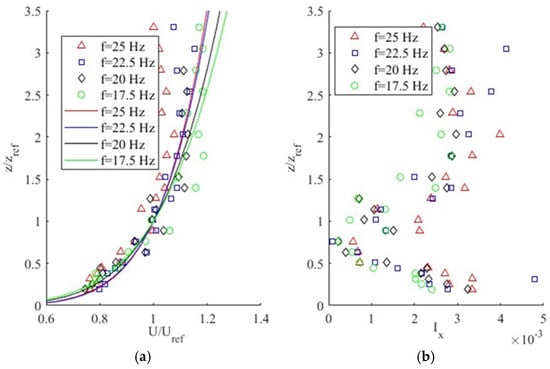
Figure 3.
(a) Velocity profile and corresponding fit. (b) Turbulent intensity profile at four different pump frequencies (f) given in Hertz in the legends. Reproduced with permission from [30].
The density of the dyed salt solution was measured using a set of hydrometers so that the specific gravity of the solution could be calculated with an uncertainty of around 5%. See [30] for more details on all the measurement methods used herein.
2.3. Experimental Procedure
For each experiment the same procedure was followed.
- The flume was turned to the desired pump frequency, and the flow rate was checked by measuring the head over the weir at the downstream end of the flume. All tests were performed using one of the four frequencies for which velocity profiles had been measured.
- Short videos were recorded with the lights and laser off and with the lights off and laser on to record values of and , respectively. This was conducted prior to each experiment as the ambient concentration of the dye increased following each experiment.
- The balloon was inflated with 300 mL of dense saline solution and then placed in the flume 10 cm upstream of the model building. The distance was measured using a metal ruler, measuring from the center of the upstream face of the model building to the center of the balloon. The center of the balloon was established by looking from directly overhead and ensuring that the two distances from the center to the balloon to the upstream and downstream edges of the balloon were equal.
- The lights were turned off one final time, and the experiment was illuminated using a flashlight. Once the video started recording, the balloon was popped using a sharp needle at the end of a long thin wooden rod. The person popping the balloon simultaneously turned off the flashlight. This allowed the release time to be logged on the video by the image going dark. The difference in time between the popping of the balloon and the flashlight being turned off was very small (of the order of a tenth of a second) and was much smaller than any other time scale associated with the experiment.
- The recording was stopped after several minutes when visual observation could no longer be used to see any of the dense fluid still trapped in the building wake.
Occasionally, small fragments of the popped balloon would either block the camera’s view or pass through the laser light sheet, producing a shadow. This occurred in fewer than 10% of the experiments, and the interference typically lasted for a single frame of the video. These frames are retained in the image analysis as they are both rare and had minimal impact on the qualitative and quantitative results.
3. Qualitative Results
Tests were run for 23 different Richardson numbers ranging from = 0 to = 32.6 using the LIF technique to measure the concentration in a vertical plane in the wake of the cube. The Richardson number (defined in equation 1) is calculated using a reference height equal to the height of the model building (h = 10 cm), and the reference velocity is the time-averaged velocity at the height of the top of the cube. Typically, three runs of each Richardson number were conducted to capture the variation across nominally identical experiments. A total of 68 tests were conducted. See Table 1 for a list of test cases.

Table 1.
List of Richardson numbers tested along with the flow velocity and number of tests for that case.
In addition to the 23 Richardson number tests that were run using LIF for concentration measurement, a subset of four Richardson number tests were run using red dye with a white background and color camera. These visualization tests were conducted to understand the full three-dimensional flow behavior and to provide context for the concentration measurements reported herein.
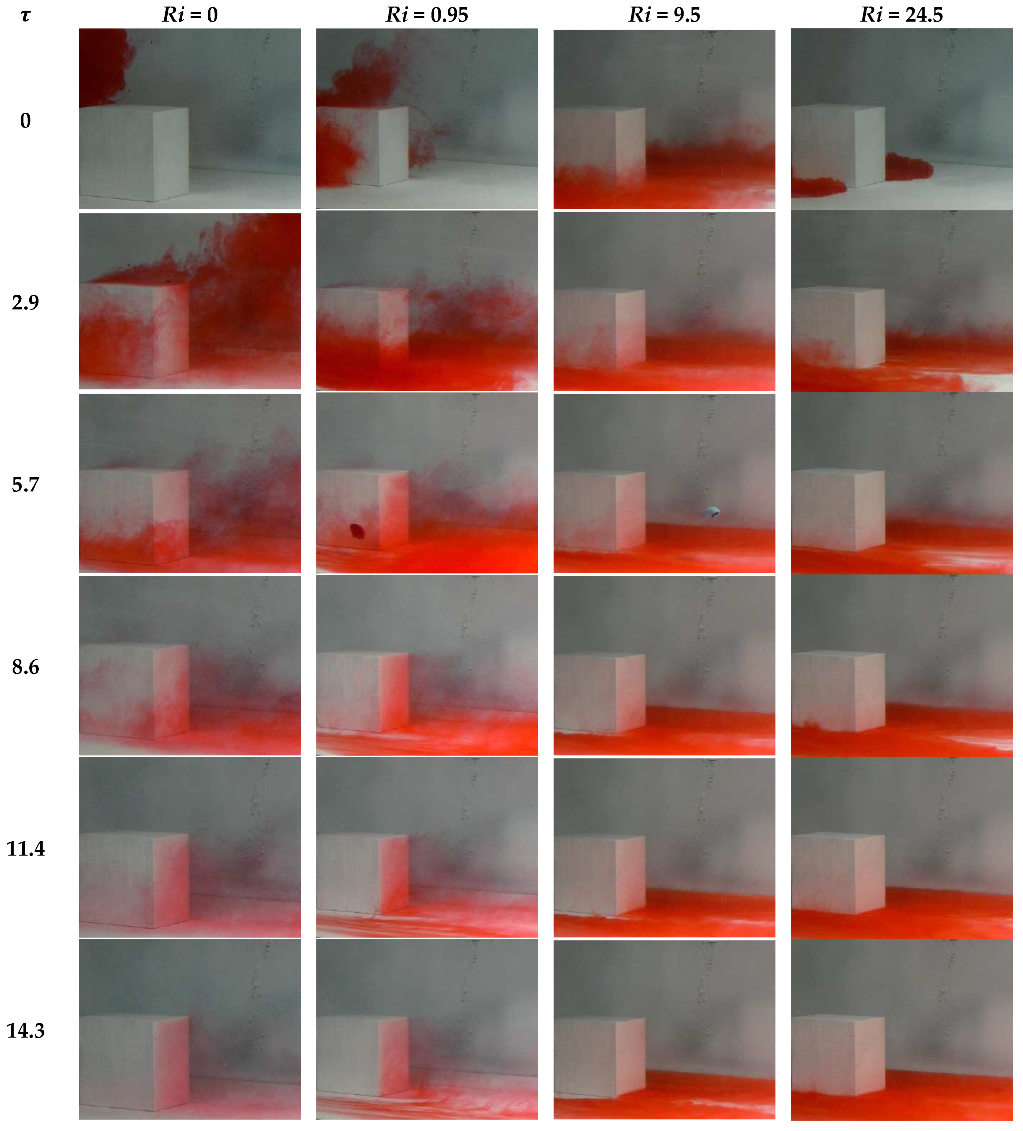
Images taken every 5 s from these visualization experiments are shown in Figure 4. There is a clear difference in behavior between flows with different Richardson numbers. For low , the flow moves over and around the cube, and there is clearly considerable mixing even before the cloud reaches the wake. For = 0 the cloud predominantly passes over the cube with some fluid drawn into the wake and then flushed out over time. However, as the increases to = 0.95, the density of the fluid begins to influence the cloud with a substantial portion now passing around the cube as it is held closer to the ground by the density of the source fluid.
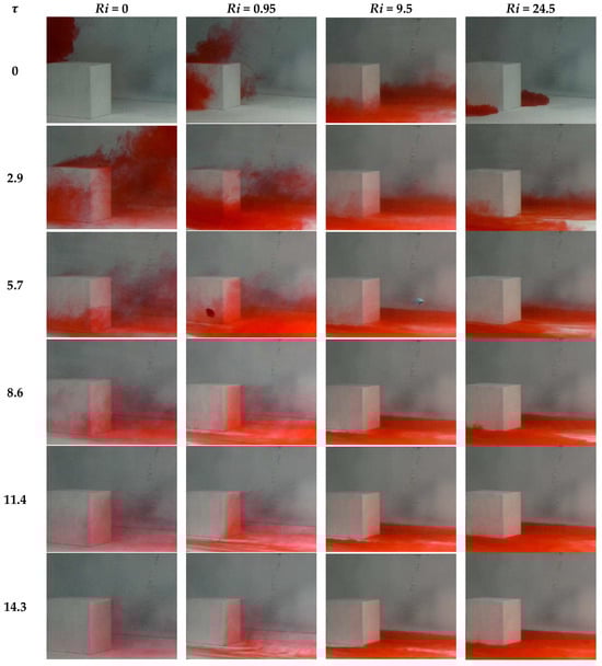
Figure 4.
Images from a series of finite release flow visualization experiments taken every (5 s in dimensional time) for a range of Richardson numbers. The objects observed in the third row of frames for the center two columns are balloon fragments. Reproduced with permission from [30].
For higher the behavior is completely different. For = 9.5 the cloud only passes around the cube and is then drawn into the wake from the sides and downwind of the cube. The dense fluid in the wake is then drawn upwind to the leeward face of the cube and flushed from the wake by being driven up the leeward face and out the top of the wake. For the highest visualized ( = 24.5), the cloud that passes around the cube is thinner than for = 9.5. In both cases the dense lower layer stays in the wake for a prolonged time. For example, in the final set of frames (bottom row of Figure 4) there is still a clear thin dense layer across the whole of the channel for the two highest . There is a more broken up layer for = 0.95, whereas the = 0 case has no such layer, though there is still some fluid trapped within the wake.
The remaining experimental results are presented in non-dimensional form. The concentration is represented by the non-dimensional reduced gravity () defined in (6). Time is scaled on the time taken to travel the reference length (h) when moving at the reference velocity. That is
For all the experiments reported herein, while the reference velocity was varied between 5.7 and 11 cm/s depending on the Richardson number being tested. The horizontal () and vertical () coordinates are measured from the base of the leeward face of the cube and are scaled on the reference length . The non-dimensional coordinates are denoted by
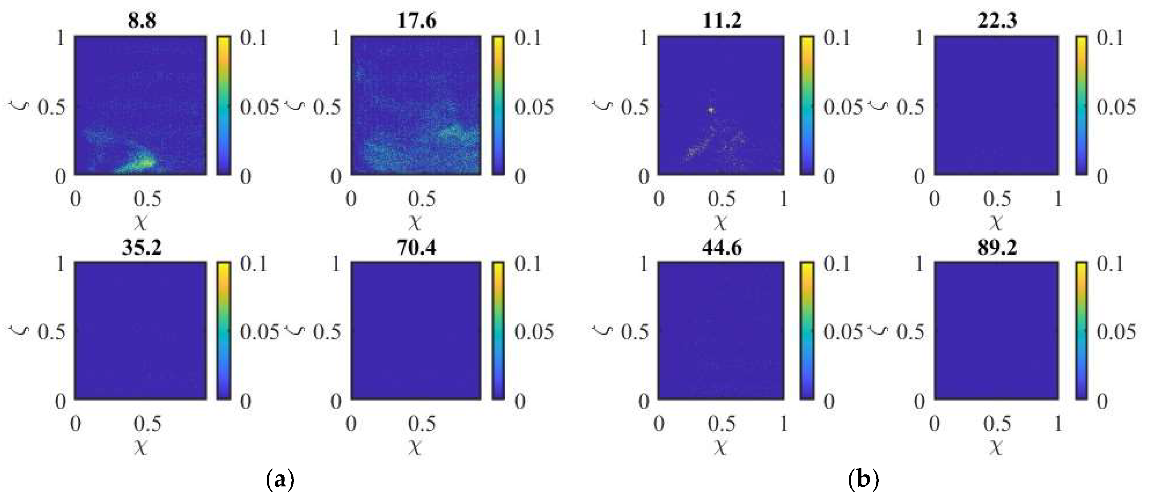
Figure 5 shows sample concentration maps for a 10 cm square section of a plane parallel to the flow aligned with the center of the cube. Contours of are shown four times for each six Richardson numbers. The same basic behavior is seen, as observed in Figure 4. For low (Figure 5a), very little dense fluid enters into the wake, while for = 2 (Figure 5b) more fluid comes around the side of the cube into the wake. When the increases to = 4 (Figure 5c), there is a clear lower dense layer in the wake of the cube, though it is flushed relatively quickly.
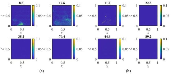
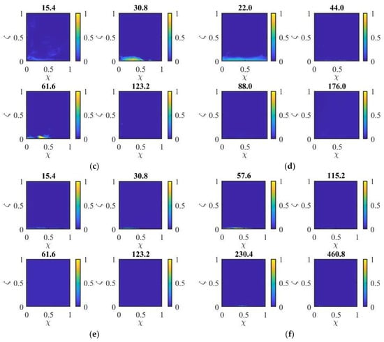
Figure 5.
Contours of non-dimensional concentration () at different non-dimensional times ( listed above each plot) for a range of Ricardson numbers: (a) = 1, (b) = 2, (c) = 4, (d) = 9, (e) = 18.3, and (f) = 32.6.
For higher ( = 18.3 and 32.6, Figure 5e,f), there is only ever a lower dense layer in the wake, which is consistent with the images in Figure 5 for = 24.5. For the highest Richardson number, the thin layer is still visible at which is the time taken for the fluid to travel 450 times the distance from the release point to the cube.
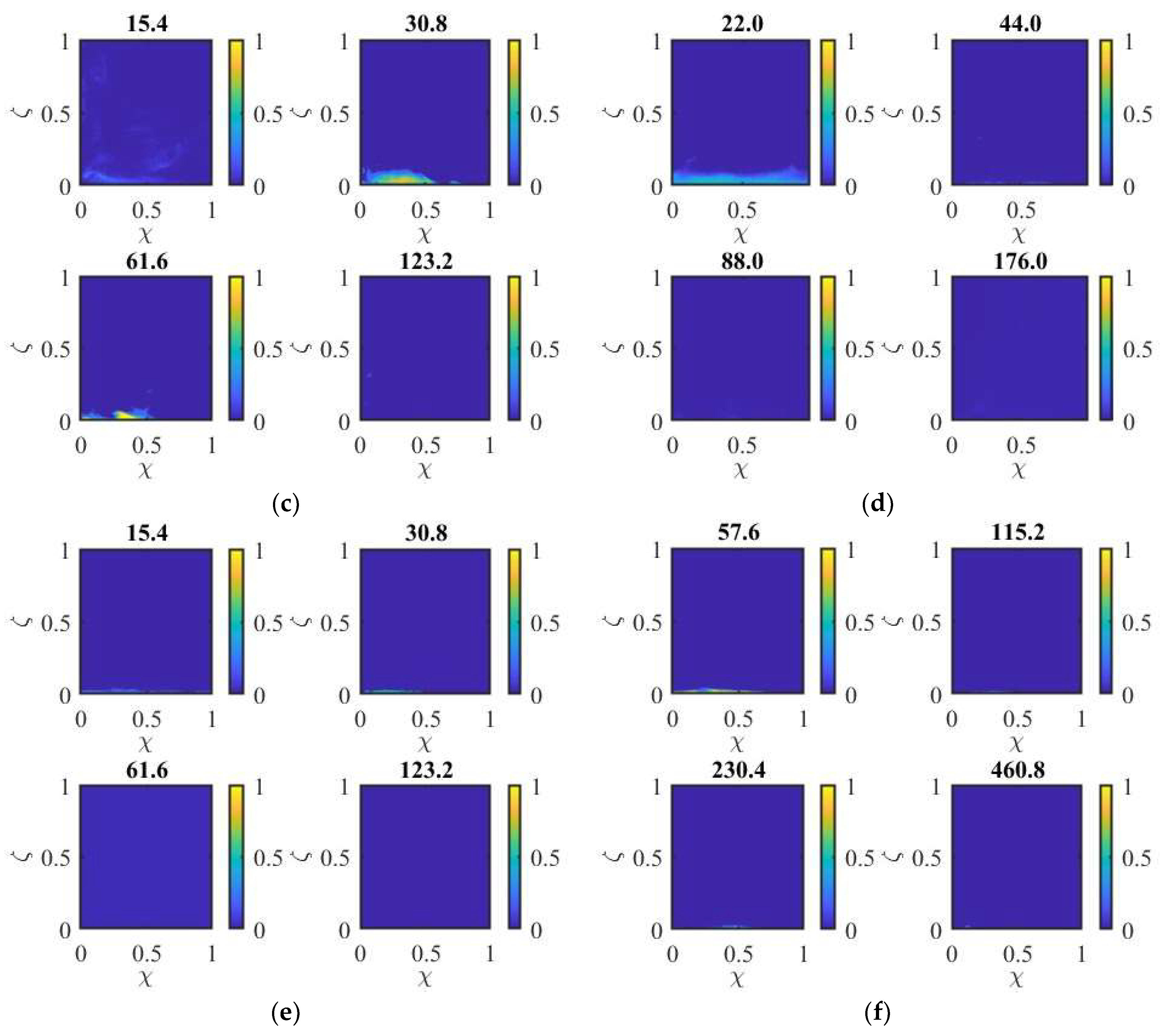
Another way to visualize the structure of the wake is to look at how the vertical profile of varies over time. To do this the vertical profile was extracted from each frame at a specific distance downstream of the leeward face of the cube and then concatenated into a contour plot. Plots were produced for the time-varying vertical profiles at downstream distances of , and for the same set of Richardson numbers presented in Figure 5. The time contours are shown in Figure 6.
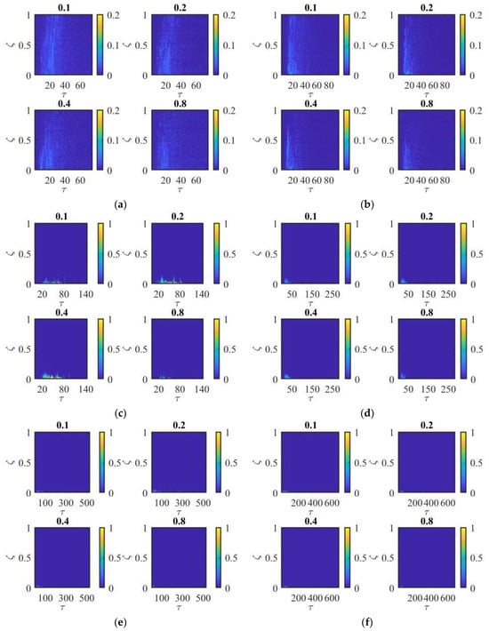
Figure 6.
Time series of vertical non-dimensional concentration () at different non-dimensional downstream distances ( listed above each plot) for a range of Ricardson numbers: (a) = 1, (b) = 2, (c) = 4, (d) = 9, (e) = 18.3, and (f) = 32.6.
For low Richardson numbers, = 1 and = 2, the wake remains vertically well mixed. While there are some variations in concentration with height, there are measurable concentrations at all heights with the concentration slowly decreasing with time. However, for larger Richardson numbers, there is typically a clear lower layer with negligible dense fluid above the layer. The transition from the well-mixed to the two-layer stratification occurs around = 4, and the layer gets thinner with increasing Ri and increasing time.
The lower dense layer seen for can take substantial time to appear. For example, for = 4 (Figure 6c) the lower layer forms at around as it takes time for the dense cloud to pass around the cube and be drawn into the wake. There are also significant fluctuations in the height of the layer over time. This is consistent with the observations report in [30] for the continuous release of dense fluid upstream of a cube. There it was observed that the flushing of the dense fluid from the wake for high Richardson numbers was due to small packets of fluid being swept off the surface of the lower layer and then transported upstream towards the leeward wall, then up and out of the wake.
4. Quantitative Results
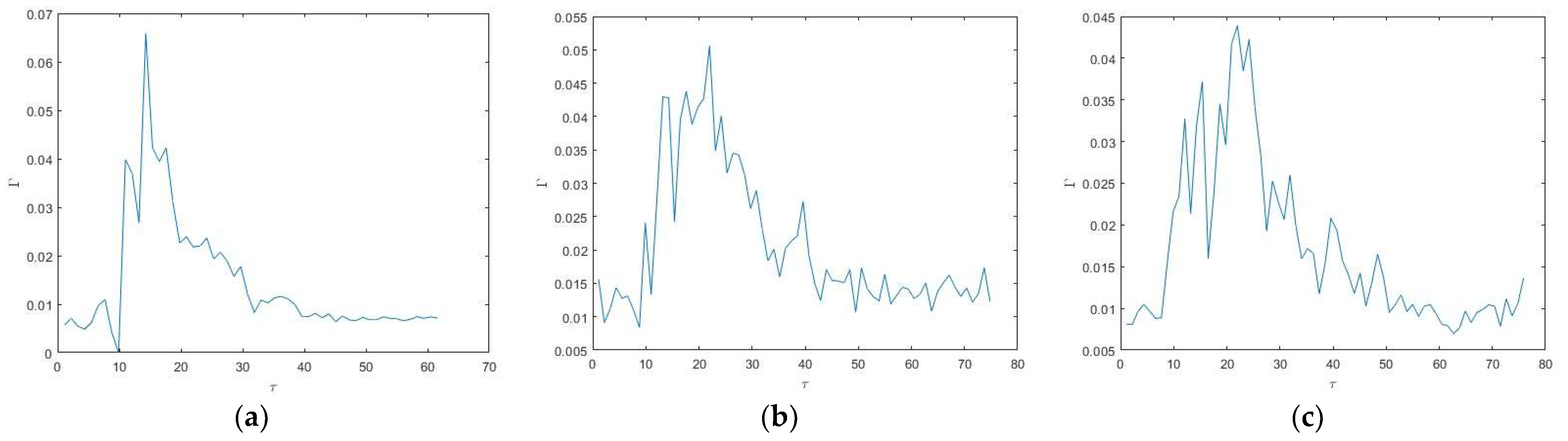
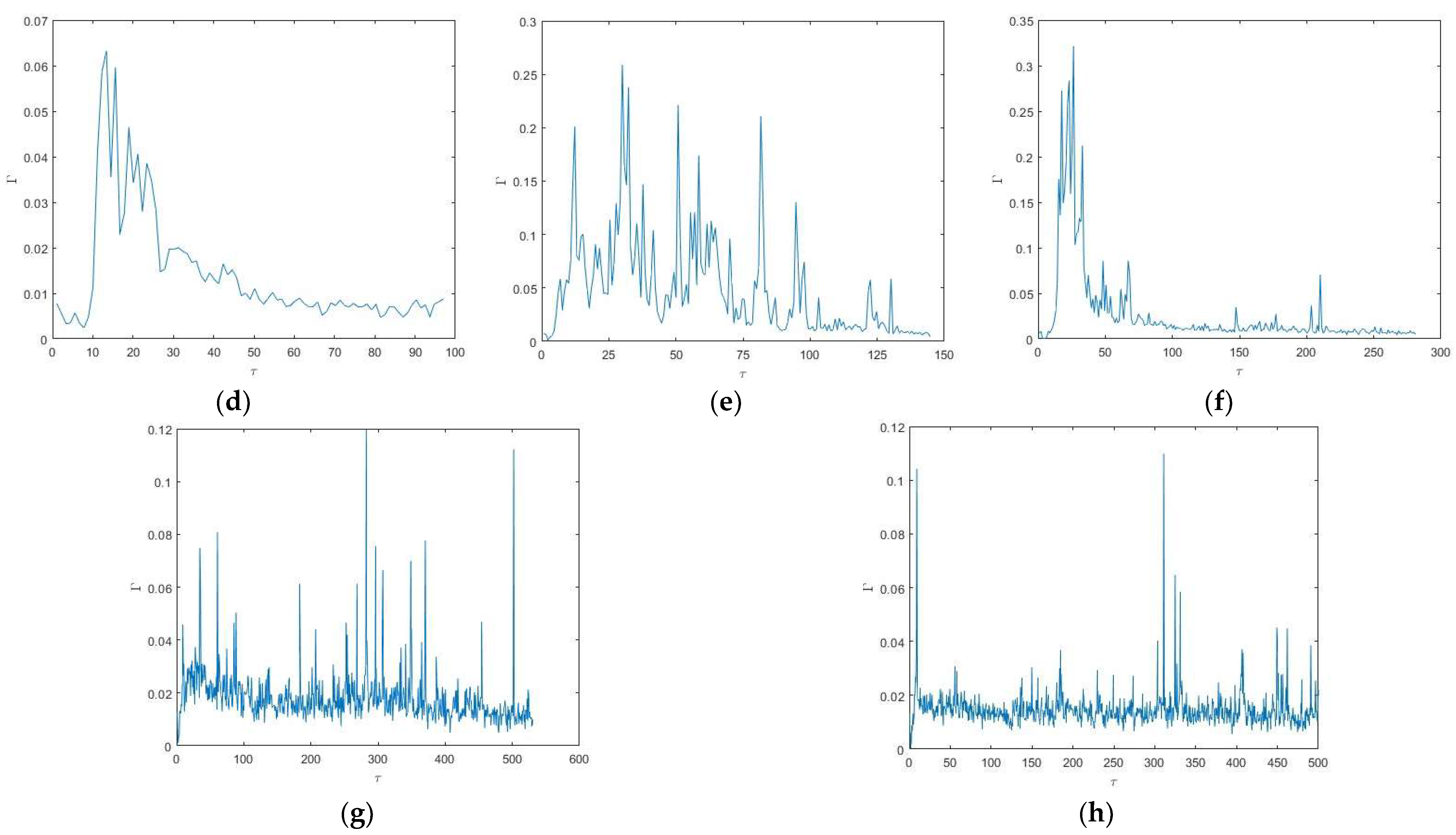
The quantitative results are focused on a particular location 1 cm above the channel floor and 1 cm downstream of the leeward building face, that is, at . This location is chosen as the same location analyzed in the prior study of continuous release of dense fluid for the same geometry [30]. The measurements reported are an area-averaged concentration over a square window with 1 mm side lengths. Again, this is to be consistent with the continuous release data presented in [30]. Measurements of the concentration over time are presented in non-dimensional form, i.e., , for a sample of Richardson numbers in Figure 7. Although all the experimental runs for a given Richardson number are nominally identical, all the data presented in Figure 7 is for the second experiment run at a particular Richardson number.
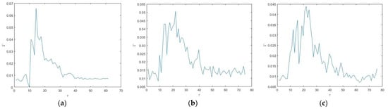
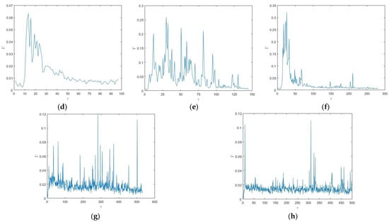
Figure 7.
Time series of non-dimensional concentration for different Richardson numbers: (a) = 0, (b) = 0.52, (c) = 1, (d) = 2, (e) = 4, (f) = 9, (g) = 18.3, and (h) = 32.6.
For small Richardson numbers ( < 4), there is an initial spike in the sharp initial increase in concentration followed by a slower decay. The initial spike is quite small with , indicating substantial mixing of the cloud prior to it being drawn into the wake. For the behavior is quite different. With one exception (), the initial peak is less pronounced. That is, it is not substantially larger than later peak fluctuations. The decay is also generally much slower than for small Richardson numbers. The baseline concentration decreases very slowly, and there are substantial spikes in concentration over time. For example, for the largest two Richardson number cases shown the baseline concentration hardly changes at all over the period . Further, these small decreases are substantially smaller than the spikes in concentration during that time. For example, for , the lower bound of decreases from around 0.02 to 0.01 over the period , whereas there are regular spikes in of up to in the same period.
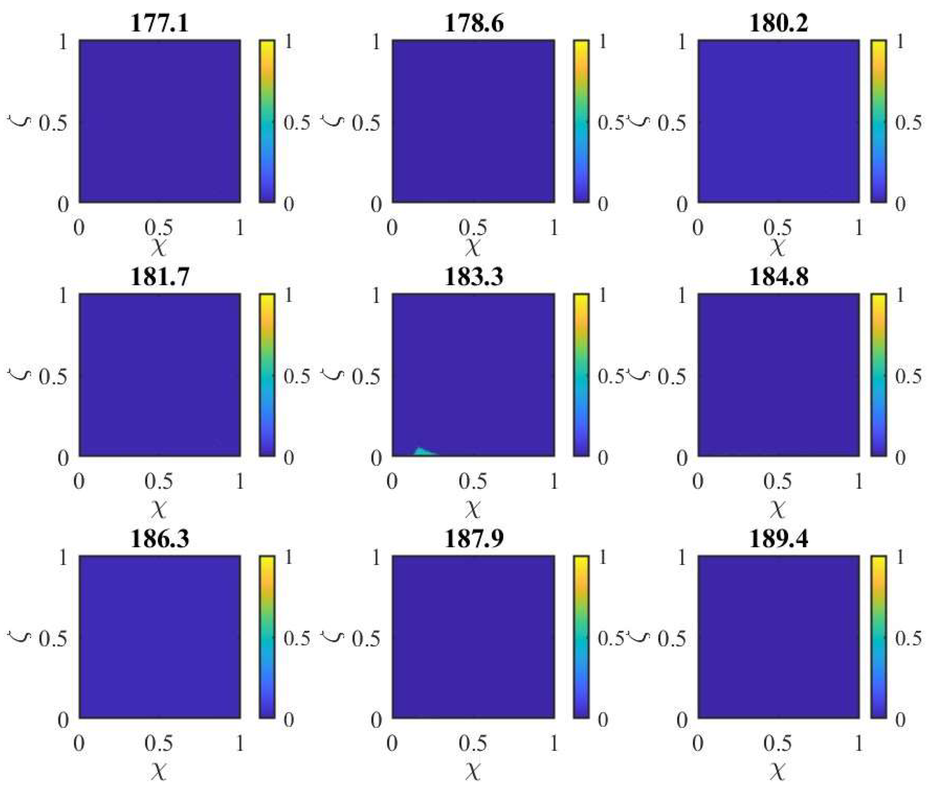
This behavior in for higher is consistent with the qualitative results discussed in the previous section. The dense cloud collapses into a thin layer that spreads out round the cube and is drawn into the wake of the cube. The flushing is then driven by dense fluid packets being swept off the top of the dense layer upwind to the cube’s leeward face, and then up and out of the wake. The spikes in the plots for larger are due to these dense patches being skimmed off the top of the layer. To illustrate this we examine in detail the spike in the plot that occurs at . Figure 8 shows consecutive experimental contours of for the frame of the spike and the four frames immediately preceding the spike and the four frames that immediately follow the spike. The figure shows a small patch of dense fluid passing over the measurement location () at the moment of the spike. The patch forms and moves rapidly and is only captured in that frame. However, the frame also shows the very thin layer at the base of the flow.
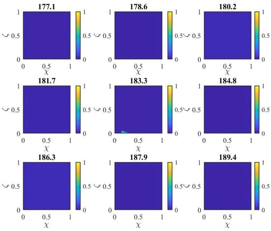
Figure 8.
Contours of non-dimensional concentration () at different non-dimensional times ( listed above each plot) for = 18.3.
The transition in behavior is seen more clearly in Figure 9, which shows the same data as Figure 7 plotted together for the low Richardson number cases ( in Figure 9a) and high Richardson number cases ( in Figure 9b). Figure 8 illustrates that there is an intermediate transitional behavior for where there are much higher peaks in the measured concentration that reach as high as . For these flows the density of the released cloud inhibits mixing during the initial collapsing of the cloud. However, when the cloud is drawn into the wake it is thick enough to reach as high as and is seen in the measurements reported in Figure 7 and Figure 9. For larger the dense layer in the wake is much thinner than , and only the spikes show up with any significant concentration.
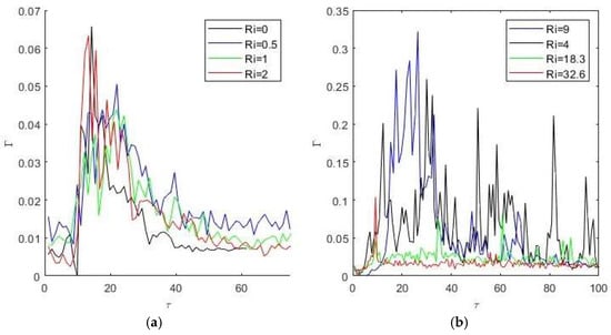
Figure 9.
Combined time series of non-dimensional concentration for different Richardson numbers: (a) low Richardson numbers () and (b) high Richardson numbers ().
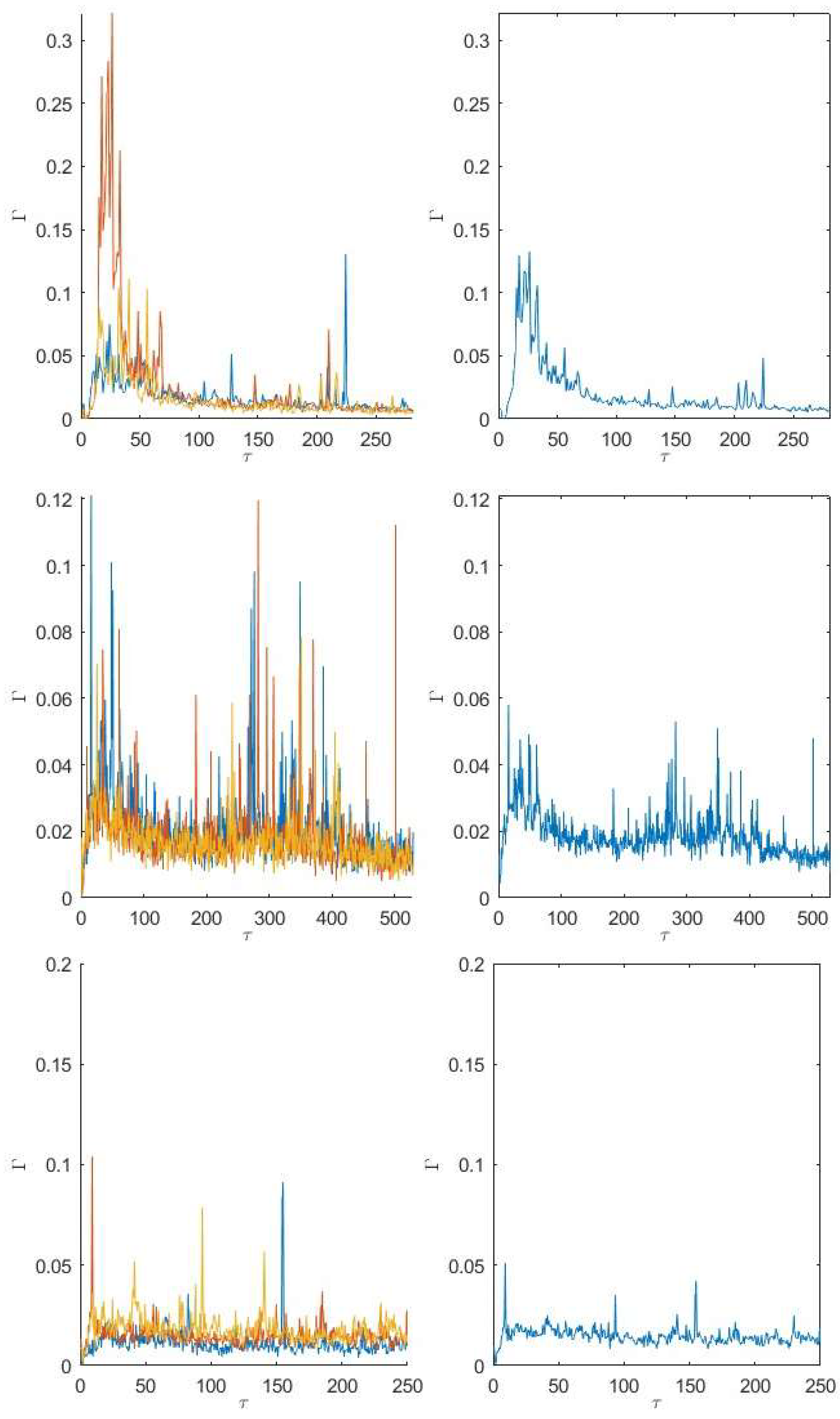
The measurements reported so far have been for individual runs for a subset of Richardson numbers. However, as shown in Table 1, multiple experiments were conducted for each case. Figure 10 and Figure 11 show plots of at (left column of each figure) and the resulting ensemble average of each case (right column of each figure). The ensemble average variation in with was calculated by taking the average of each test’s concentration values measured at each time where the time was measured from the instant the dense fluid was released. These figures illustrate the variability between individual realizations of the same experiment, which can be substantial.
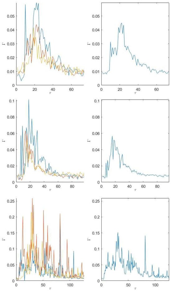
Figure 10.
Time series of at showing (left) each experimental run and (right) the ensemble average of all experimental runs. From top to bottom, = 1, 2, and 4.

Figure 11.
Time series of at , showing (left) each experimental run and (right) the ensemble average of all experimental runs. From top to bottom, = 9, 18.3, and 32.6.
For all cases there is substantial variation from one experiment to the next. For low Richardson numbers (), there are major differences in both the timing and magnitude of the initial peak, though the subsequent decay is more consistent from experiment to experiment. For example, for , the peaks vary from and the time of the peak varies from . However, for there is very little variation between the different runs.
For the transitional Richardson numbers , the variation is even larger. For example, for the peaks vary from . For these cases it is also harder to identify a clear initial peak and decay as there can be multiple initial peaks with substantial drops in between the peaks. For example, for one case (orange line) has a clear peak of followed by a drop to before rising up again to . While the ensemble average for shows a clear peak and decay, this is not seen anywhere near as clearly in the individual experimental runs.
Higher Richardson numbers () also show variability, though much of this is due to the timing of the large intermittent spikes caused by parcels of dense fluid being peeled off the top of the dense layer and transported upstream, as illustrated in Figure 8.
The mean behavior and the variability around that mean are illustrated in Figure 12. This shows the measured peak concentration and the time of the peak concentration for each experiment and all 23 Richardson numbers (left column of Figure 12). Also shown is the arithmetic mean of those measurements and the values derived from the ensemble averages. In all cases the mean value of is always greater than the peak value of the ensemble mean. This is because the peak values in the individual tests occur at different times. The mean value of is small for small Richardson numbers () and then jumps substantially for the transitional experiments () before reducing again for larger . The same is true for the timing of the peak. For the peaks all occur for which jumps as high as for before dropping back to around for higher .
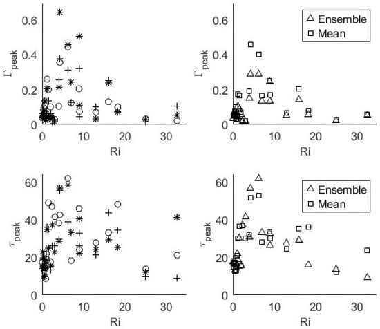
Figure 12.
Summary plots of peak of (top row) and time for peak (bottom row) at . Left column is the data from each experimental run (each symbol representing a different run at the same ), and the right column is the mean and ensemble average values across all experimental runs.
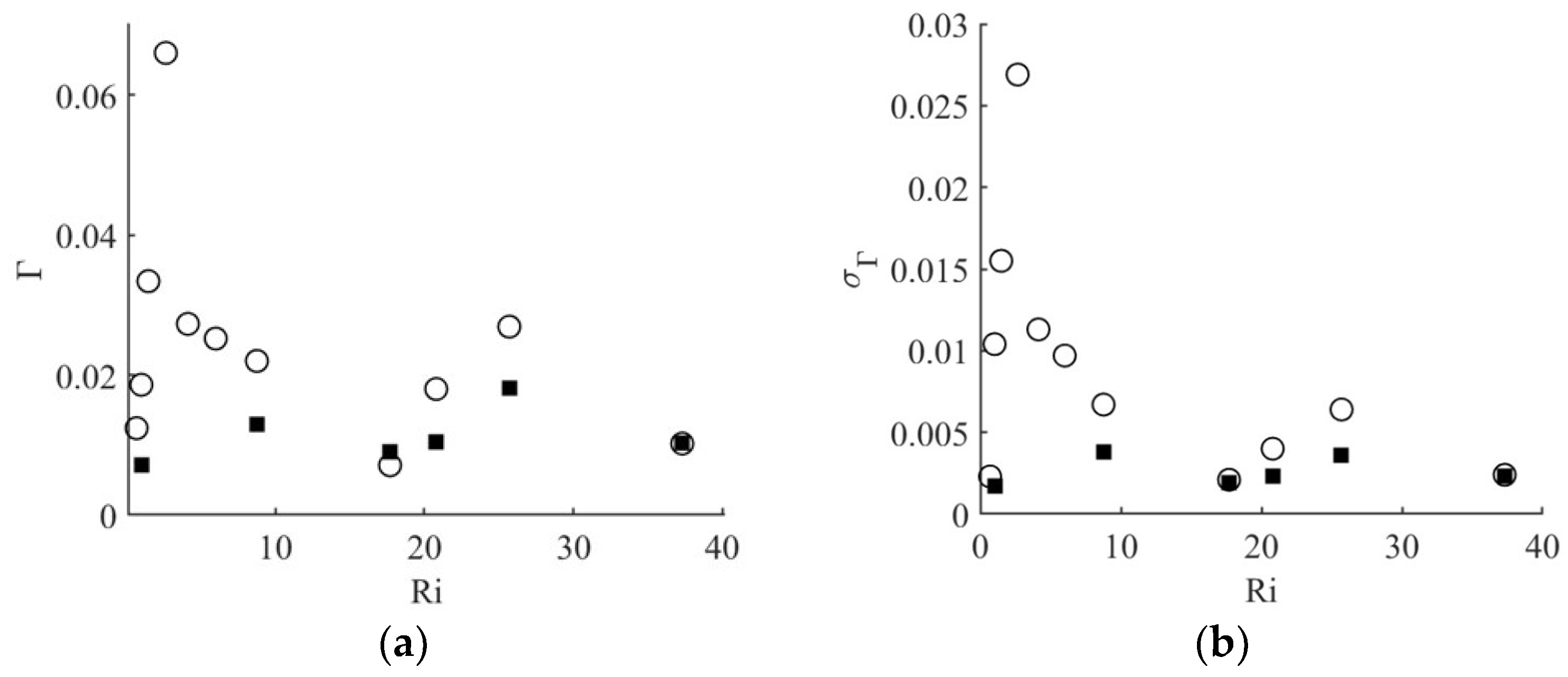
For comparison, the mean and standard deviation of measured at the same location but for continuous release tests [30] are shown in Figure 13. The same qualitative behavior is observed. For small the concentration is small. It then sharply increases with increasing before slowly reducing as gets larger. However, there are two quantitative differences. First, the ensemble average values of for the finite release tests are substantially larger than the mean values for continuous release tests. Second, the largest value of time-averaged occurs at a much lower Richardson number () compared to the finite release tests reported on herein (). The most likely explanation for this is related to the release location. For both the finite and continuous release tests, the dense fluid was released 10 cm upstream of the cube. However, for the continuous release test, the dense fluid was released from ground level, whereas, for the finite release tests, the dense fluid was released from a balloon with a diameter of around 5–6 cm. Therefore, during the initial release after the balloon popped, the dense cloud collapsed down as it was swept forward. There is, therefore, likely to be substantial mixing during this process for low to intermediate Richardson numbers. The peak in the finite release tests is likely controlled in part by the level of mixing in the collapsing stage of the release, with higher leading to less slumping mixing. This would likely result in the peak concentration occurring at higher compared to the continuous release tests that did not have the slumping phase. It is also interesting to note that the variability in the continuous release tests also peaks near the peak in the mean. This is qualitatively similar to the observed variability in the finite release tests.
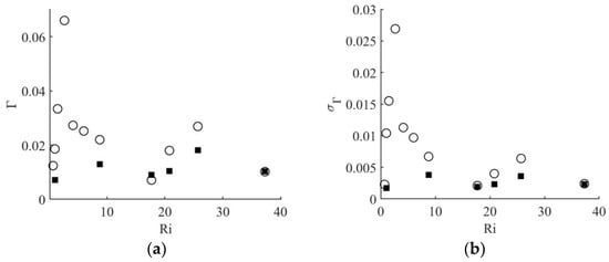
Figure 13.
Plot of the mean (a) and standard deviation (b) of concentration as a function of source Richardson number for continuous release experiments for different source flow rates (Q). Q = 400 mL/min—circle and Q = 200 mL/min—solid. Reproduced with permission from [30].
5. Discussion
The visualization experiments shown in Figure 4 show distinct differences between low and high Richardson number flows. For high Richardson numbers the dense cloud collapses and forms a thin layer of dense fluid at ground level which is then drawn into the cube wake. Parcels of dense fluid are then skimmed off the surface of the dense layer and transported upstream toward the leeward wall of the cube. This is consistent with the broad flow structure observed for flow around an isolated cube seen schematically in Figure 14. The horseshoe vortex that forms around the perimeter of the leeward wall draws fluid into the wake as it passes around the cube. This vortex also generates an upwind flow within the wake at ground level that approaches the leeward wall and then moves up the wall driving dense fluid up and out of the wake.
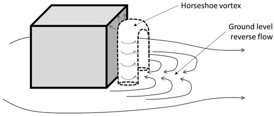
Figure 14.
Schematic diagram of some features of the flow in the wake of a surface-mounted cube showing the horseshoe vortex (dashed lines) and reverse flow back toward the cube. Modified with permission from [30].
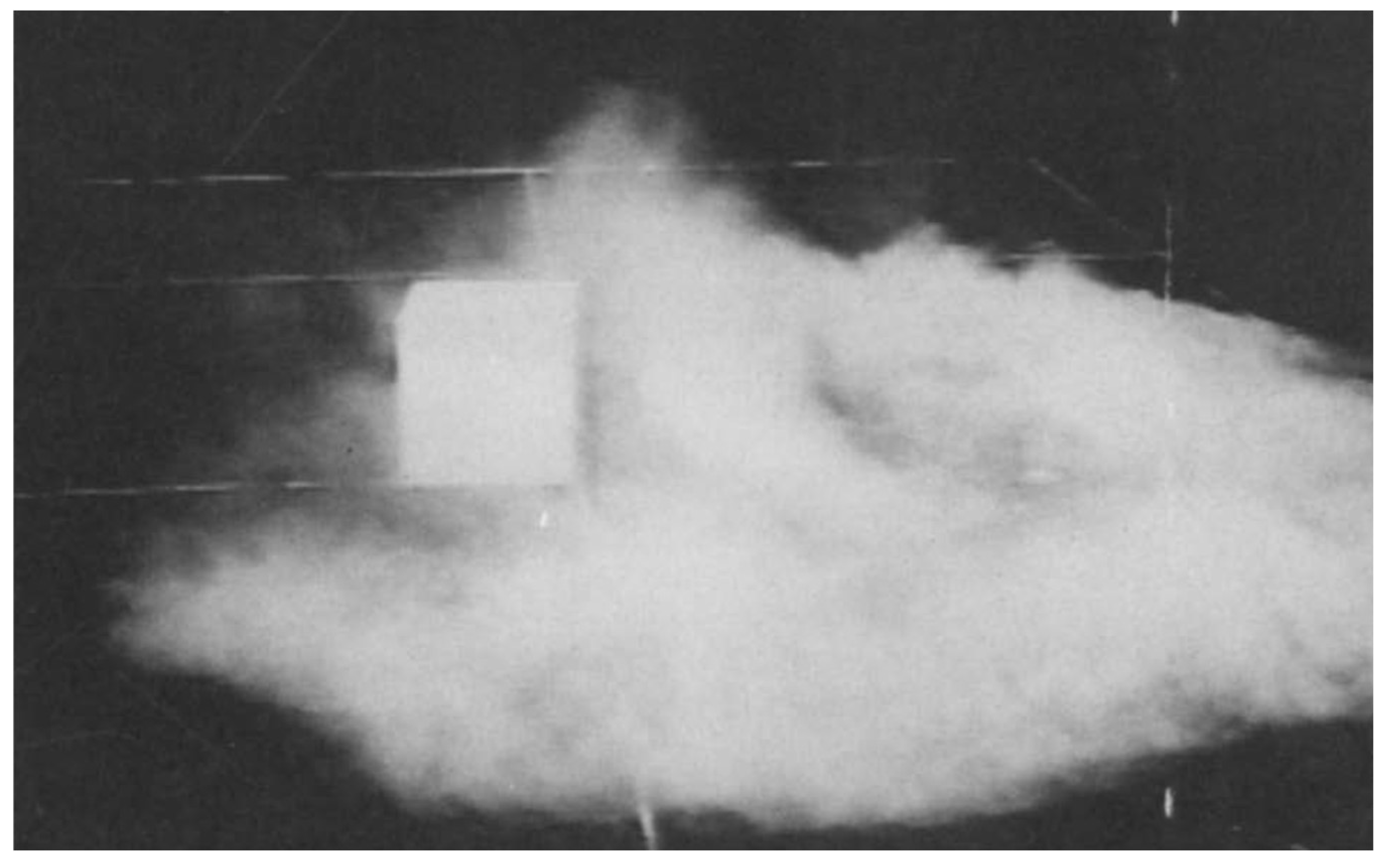
The goal of this study is to provide detailed experimental data for the dispersion of dense gas as it flows around a cubic building downwind of the release location. However, the scale of the experiments is several orders of magnitude smaller than full-scale occurrences. To overcome this problem the tests were run in water, which has a kinematic viscosity an order of magnitude smaller than that of air. The tests were also run at Reynolds numbers high enough to be in the Reynolds number independent regime for this type of flow. As a final validation check, we compare the visualization images from Figure 4 with photos from the Thorney Island tests and wind tunnel simulations of the same tests. These images are shown in Figure 15 and Figure 16.

Figure 15.
Image of a wind tunnel simulation of test 028 from Thorney Island Phase II for a cloud with a Richardson number of = 1.5. Reproduced with permission from [56].
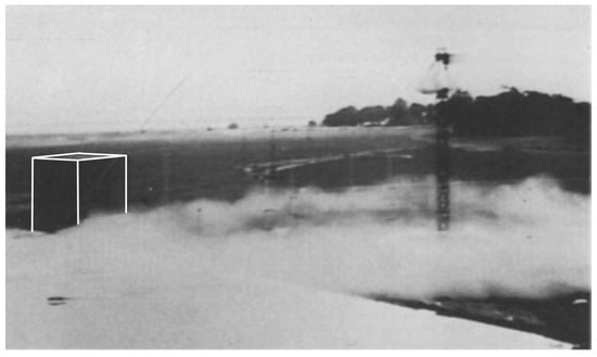
Figure 16.
Image of test 026 from Thorney Island Phase II for a cloud with a Richardson number of = 34.8. Reproduced with permission from [56]. The building is on the far left of the image and shows the dense cloud going around the building with a height substantially below that of the building. The image has been altered by adding white lines to highlight the outline of the building.
Figure 15 shows an image from a large wind tunnel simulation of test 28 from the Thorney Island Phase II tests. The image shows the dense cloud engulfing the model building in a manner similar to the low Richardson number cases in Figure 4. The Richardson number for this test in Figure 15 is = 1.5, which is in the low Richardson number range identified in the present study.
Conversely, Figure 16 shows an image from the full-scale Thorney Island Phase II tests for a high Richardson number flow ( = 34.8). Here the dense cloud collapses and flows around the building. This is consistent with the small-scale visualization test for = 24.5 shown in Figure 4. In both images the cloud is about 10–20% of the height of the building as it passes around, and no dense fluid is observed to flow up and over the building.
Despite the large difference in scale between the Thorney Island experiments (10 m cubic building) and the experimental results presented herein (10 cm cubic building), the same flow patterns are observed, and the distinction between low and high Richardson number cases is identical. This visual agreement strongly suggests that the small-scale experiments presented herein are capturing the main physical processes present in dense gas dispersion in urban areas.
6. Conclusions
A series of small-scale experiments were conducted to simulate the dispersion of a finite release of dense gas upwind of an isolated building. The main goal of the paper was to develop a large set of concentration data across a broad range of flow Richardson numbers that could be used as a model validation tool for computational models of dense gas dispersion. To achieve this goal a series of tests were run to replicate the geometry of the Thorney Island dense gas dispersion tests with much higher spatial and temporal resolution measurements than were possible with the field tests.
The experimental results showed two distinct flow regimes for low and high Richardson numbers. For low (), the dense gas cloud flows around the building and, while dense fluid is drawn into the building wake, it is rapidly flushed out. For high (), the cloud collapses and flows around the building with dense gas being drawn into the wake at ground level. Flushing is then achieved by small parcels of fluid being skimmed off the top of the dense layer, transported upstream to the leeward wall of the building, and then up and out of the wake. This process is much slower and intermittent compared to the low Ri case. The transition between these two regimes is marked by much higher concentrations in the wake and much larger variability between runs for nominally identical experiments. The flow regimes identified in the small-scale experiments are also observed in the full-scale Thorney Island tests.
The results presented are for a finite release of dense fluid upstream of a cubic building. While tests were run for a broad range of Richardson numbers, other parameters were held constant. In all cases the dense gas release had a volume of 300 mL (30% of the volume of the model building) and was released such that the center of the release volume was 10 cm upstream of the windward face of the building. Future work is needed to understand the impacts these two parameters (release distance and release volume) have on the flow and dispersion.
Author Contributions
Conceptualization, N.K.; methodology, N.K. and R.A.; software, R.A. and N.K.; validation, R.A.; formal analysis, R.A. and N.K.; investigation, R.A.; resources, N.K.; data curation, R.A.; writing—original draft preparation, R.A. and N.K.; writing—review and editing, N.K. and R.A.; visualization, R.A. and N.K.; supervision, N.K.; project administration, N.K.; funding acquisition, N.K. All authors have read and agreed to the published version of the manuscript.
Funding
This work was funded by the U.S. National Science Foundation (NSF) under Grant No. 1703548.
Data Availability Statement
The raw data supporting the conclusions of this article will be made available by the authors upon request.
Acknowledgments
The authors would like to thank Daniel Metz, Scott Black, and Caleb Jackson for their technical support in building the test rigs. This material is based upon work supported by the National Science Foundation (NSF) under Grant No. 1703548. Any opinions, findings, and conclusions or recommendations expressed in the material are those of the authors and do not necessarily reflect the views of the NSF.
Conflicts of Interest
The authors declare no conflicts of interest.
References
- United Nations. U.N. Population Fund. Available online: https://www.unfpa.org/urbanization (accessed on 23 April 2025).
- Goodfellow, H.; Tahti, E. (Eds.) Industrial Ventilation Design Guidebook; Elsevier: Amsterdam, The Netherlands, 2001. [Google Scholar]
- Baratian-Ghorghi, Z.; Kaye, N.B. Flushing a finite volume of dense fluid from a square street canyon by a turbulent over-flow. Atmos. Environ. 2012, 60, 392–402. [Google Scholar] [CrossRef]
- Buckley, R.L.; Hunter, C.H.; Addis, R.P.; Parker, M.J. Modeling dispersion from toxic gas released after a train collision in Graniteville, SC. J. Air Waste Manag. Assoc. 2007, 57, 268–278. [Google Scholar] [CrossRef]
- Bhopal Disaster. Available online: https://en.wikipedia.org/wiki/Bhopal_disaster (accessed on 23 April 2025).
- Pannett, R. Chlorine Gas Leak at Jordan’s Aqaba Port Kills at Least 13, Injures Hundreds. Washington Post. 2022. Available online: https://www.washingtonpost.com/world/2022/06/28/jordan-toxic-gas-leak-chlorine-aqaba/ (accessed on 26 September 2024).
- Louisiana Illuminator. 2 Toxic Releases in Louisiana Under Federal Investigation for Safety Recommendations. 2024. Available online: https://lailluminator.com/2024/04/06/toxic-releases/ (accessed on 26 September 2024).
- ABC-13 Houston. At Least 7 Children Hospitalized After Chlorine Leak in Lazy River at Memorial Area Club, HFD Says. 2023. Available online: https://abc13.com/chemical-spill-chlorine-exposure-wilcrest-drive-club-westside/13423128/ (accessed on 26 September 2024).
- Winkle, K.; Ramkisson, J. Downtown Austin Building Evacuated After Chlorine Gas Released. KXAN News. 2020. Available online: https://www.kxan.com/news/breaking-news/downtown-austin-building-evacuated-after-chlorine-gas-released/ (accessed on 26 September 2024).
- Kay, J. Chlorine Accidents Take a Big Human Toll. Environmental Health News. 2011. Available online: https://www.ehn.org/chlorine-accidents-take-a-big-human-toll-2565934161.html (accessed on 26 September 2024).
- Brown, M.J.; Nelson, M.A.; Williams, M.D.; Gowardhan, A.; Pardyjak, E.R. A non-CFD modeling system for computing 3D wind and concentration fields in urban environments. In Proceedings of the Fifth International Symposium on Computational Wind Engineering (CWE2010), Chapel Hill, NC, USA, 23–27 May 2010. [Google Scholar]
- Fthenakis, V.M. HGSYSTEM: A review, critique, and comparison with other models. J. Loss Prev. Proc. Ind. 1999, 12, 525–531. [Google Scholar] [CrossRef]
- Spicer, T.; Havens, J. User’s Guide for the DEGADIS 2.1 Dense Gas Dispersion Model; Technical Report No. EPA-450/4-89-019; Environmental Protection Agency: New York, NY, USA, 1989. [Google Scholar]
- Morgan, D.L.; Morris, L.; Ermak, D. SLAB: A Time-Dependent Computer Model for the Dispersion of Heavy Gas Released in the Atmosphere; Technical Report No. UCRL-53383; Lawrence Livermore National Laboratory: Livermore, CA, USA, 1993. [Google Scholar]
- Xu, X.; Yang, Q.; Yoshida, A.; Tamura, Y. Characteristics of pedestrian-level wind around super-tall buildings with various configurations. J. Wind. Eng. Ind. Aerodyn. 2017, 166, 61–73. [Google Scholar] [CrossRef]
- Mittal, H.; Sharma, A.; Gairola, A. A review on the study of urban wind at the pedestrian level around buildings. J. Build. Eng. 2018, 18, 154–163. [Google Scholar] [CrossRef] [PubMed]
- White, B.R. Analysis and wind-tunnel simulation of pedestrian-level winds in San Francisco. J. Wind. Eng. Ind. Aerodyn. 1992, 44, 2353–2364. [Google Scholar] [CrossRef]
- Zaki, S.A.; Shuhaimi, S.S.; Mohammad, A.F.; Ali, M.S.M.; Jamaludin, K.R.; Ahmad, M.I. Development of a prediction model of the pedestrian mean velocity based on LES of random building arrays. Buildings 2022, 12, 1362. [Google Scholar] [CrossRef]
- Okaze, T.; Ono, A.; Mochida, A.; Kannuki, Y.; Watanabe, S. Evaluation of turbulent length scale within urban canopy layer based on LES data. J. Wind. Eng. Ind. Aerodyn. 2015, 144, 79–83. [Google Scholar] [CrossRef]
- Ramirez, N.; Afshari, A.; Norford, L. Validation of simplified urban-canopy aerodynamic parametrizations using a numerical simulation of an actual downtown area. Bound.-Layer Meteorol. 2018, 168, 155–187. [Google Scholar] [CrossRef]
- Hertwig, D.; Efthimiou, G.C.; Bartzis, J.G.; Leitl, B. CFD-RANS model validation of turbulent flow in a semi-idealized urban canopy. J. Wind. Eng. Ind. Aerodyn. 2012, 111, 61–72. [Google Scholar] [CrossRef]
- Boeing, G. Urban spatial order: Street network orientation, configuration, and entropy. Appl. Netw. Sci. 2019, 4, 67. [Google Scholar] [CrossRef]
- da Silva, M.T.Q.S.; do Rocio Cardoso, M.; Veronese, C.M.P.; Mazer, W. Tortuosity: A brief review. Mater. Today Proc. 2022, 58, 1344–1349. [Google Scholar] [CrossRef]
- Sulebak, J.R. Fractal analysis of surface topography. Nor. Geogr. Tidsskr.—Nor. J. Geogr. 1999, 53, 213–225. [Google Scholar] [CrossRef]
- Encarnacao, S.; Gaudiano, M.; Santos, F.C.; Tenedorio, J.A.; Pacheco, J.M. Fractal cartography of urban areas. Sci. Rep. 2012, 2, 527. [Google Scholar] [CrossRef] [PubMed]
- Hanna, S.R.; Hansen, O.R.; Ichard, M.; Strimaitis, D. CFD model simulation of dispersion from chlorine railcar releases in industrial and urban areas. Atmos. Environ. 2009, 43, 262–270. [Google Scholar] [CrossRef]
- Lamberti, G.; Garcia-Sanchez, C.; Sousa, J.; Gorle, C. Optimizing turbulent inflow conditions for large-eddy simulations of the atmospheric boundary layer. J. Wind. Eng. Ind. Aerodyn. 2018, 177, 32–44. [Google Scholar] [CrossRef]
- Hwang, Y.; Gorlé, C. Large-eddy simulations of wind-driven cross-ventilation, Part I: Validation and Sensitivity Study. Front. Built Environ. Sect. Wind. Eng. Sci. 2022, 8, 911005. [Google Scholar] [CrossRef]
- Geleta, T.N.; Bitsuamlak, G. Validation metrics and turbulence frequency limits for LES-based wind load evaluation for low-rise buildings. J. Wind. Eng. Ind. Aerodyn. 2022, 231, 105210. [Google Scholar] [CrossRef]
- Akhter, R.; Kaye, N.B. Measurements of Wake Concentration from the Continuous Release of a Dense Fluid Upstream of a Cubic Obstacle. Fluids 2025, 10, 46. [Google Scholar] [CrossRef]
- Baratian-Ghorghi, Z.; Kaye, N.B. Modeling the purging of dense fluid from a street canyon driven by an interfacial mixing flow and skimming flow. Phys. Fluids 2013, 25, 076603. [Google Scholar] [CrossRef]
- Strang, E.J.; Fernando, H.J.S. Shear-induced mixing and transport from a rectangular cavity. J. Fluid Mech. 2004, 520, 23–49. [Google Scholar] [CrossRef]
- Puttock, J.S.; Colenbrander, G.W. Thorney Island data and dispersion modelling. J. Hazard. Mater. 1985, 11, 381–397. [Google Scholar] [CrossRef]
- Hanna, S.R.; Chang, J.C.; Huq, P. Observed chlorine concentrations during Jack Rabbit I and Lyme Bay field experiments. Atmos. Environ. 2016, 125, 252–256. [Google Scholar] [CrossRef]
- Fox, S.; Hanna, S.; Mazzola, T.; Spicer, T.; Chang, J.; Gant, S. Overview of the Jack Rabbit II (JR II) field experiments and summary of the methods used in the dispersion model comparisons. Atmos. Environ. 2022, 269, 118783. [Google Scholar] [CrossRef]
- Selected Video Clips of the Thorney Island Dense-Gas Dispersion Experiments. Available online: https://www.youtube.com/watch?v=z3zjh2NsdTU (accessed on 8 March 2024).
- Johnson, D.R. Thorney Island trials: Systems development and operational procedures. J. Hazard. Mater. 1985, 11, 35–64. [Google Scholar] [CrossRef]
- McQuaid, J.; Roebuck, B. Large Scale Field Trials on Dense Vapour Dispersion; Report No. EUR 10029 (EN); Commission of the European Communities: Luxembourg, 1985; pp. 200–204+262–267. [Google Scholar]
- Sklavounos, S.; Rigas, F. Validation of turbulence models in heavy gas dispersion over obstacles. J. Hazard. Mater. A 2004, 108, 9–20. [Google Scholar] [CrossRef]
- Hall, D.J.; Waters, R.A. Wind tunnel model comparisons with the Thorney island dense gas release field trials. J. Hazard. Mater. 1985, 11, 209–235. [Google Scholar] [CrossRef]
- Spicer, T.O.; Havens, J.A. Modeling the Phase I Thorney Island experiments. J. Hazard. Mater. 1985, 11, 237–260. [Google Scholar] [CrossRef]
- Deaves, D.M. Three-dimensional model predictions for the upwind building trial of Thorney Island phase II. J. Hazard. Mater. 1985, 11, 341–346. [Google Scholar] [CrossRef]
- Hanna, S. Meteorological data recommendations for input to dispersion models applied to Jack Rabbit II trials. Atmos. Environ. 2020, 235, 117516. [Google Scholar] [CrossRef]
- Spicer, T.O.; Tickle, G. Simplified source description for atmospheric dispersion model comparison of the Jack Rabbit II chlorine field experiments. Atmos. Environ. 2021, 244, 117866. [Google Scholar] [CrossRef]
- Hanna, S.R.; Britter, R.; Argenta, E.; Chang, J. The Jack Rabbit chlorine release experiments: Implications of dense gas removal from a depression and downwind concentrations. Atmos. Environ. 2012, 213–214, 406–412. [Google Scholar] [CrossRef]
- Mazzola, T.; Hanna, S.; Chang, J.; Bradley, S.; Meris, R.; Simpson, S.; Miner, S.; Gant, S.; Weil, J.; Harper, M.; et al. Results of comparisons of the predictions of 17 dense gas dispersion models with observations from the Jack Rabbit II chlorine field experiment. Atmos. Environ. 2021, 244, 117887. [Google Scholar] [CrossRef]
- Fares, S.S. Wind Tunnel Modeling of Jack Rabbit II Mock Urban Environment Gas Concentration Measurements. Master’s Thesis, University of Arkansas, Fayetteville, AR, USA, 2022. Available online: https://scholarworks.uark.edu/etd/4621 (accessed on 10 February 2025).
- Allgayer, D.M.; Hunt, G.R. On the application of the light-attenuation technique as a tool for non-intrusive buoyancy measurements. Exp. Therm. Fluid Sci. 2012, 38, 257–261. [Google Scholar] [CrossRef]
- Crimaldi, J.P. Planar laser induced fluorescence in aqueous flows. Exp. Fluids 2008, 44, 851–863. [Google Scholar] [CrossRef]
- Debler, W.; Armfield, S.W. The purging of saline water from rectangular and trapezoidal cavities by an overflow of turbulent sweet water. J. Hydraul. Res. 1997, 35, 43–62. [Google Scholar] [CrossRef]
- Kirkpatrick, M.P.; Armfield, S.W.; Williamson, N. Shear driven purging of negatively buoyant fluid from trapezoidal de-pressions and cavities. Phys. Fluids 2012, 24, 025106. [Google Scholar] [CrossRef]
- Armfield, S.W.; Debler, W. Purging of density stabilized basins. Int. J. Heat Mass Transf. 1993, 36, 519–530. [Google Scholar] [CrossRef]
- Kirkpatrick, M.P.; Armfield, S.W. Experimental and large eddy simulation results for the purging of salt water from a cavity by an overflow of fresh water. Int. J. Heat Mass Transf. 2005, 48, 341–359. [Google Scholar] [CrossRef]
- Baratian-Ghorghi, Z.; Kaye, N.B. Shear driven flushing of dense fluid from a canyon. J. Vis. 2013, 16, 29–37. [Google Scholar] [CrossRef]
- Baratian-Ghorghi, Z.; Kaye, N.B. The effect of canyon aspect ratio on flushing of dense pollutants from an isolated street canyon. Sci. Total Environ. 2013, 443, 112–122. [Google Scholar] [CrossRef]
- Davies, M.E.; Singh, S. The Phase II Trials: A Data Set on the Effect of Obstructions. J. Hazard. Mater. 1985, 11, 301–323. [Google Scholar] [CrossRef]


Disclaimer/Publisher’s Note: The statements, opinions and data contained in all publications are solely those of the individual author(s) and contributor(s) and not of MDPI and/or the editor(s). MDPI and/or the editor(s) disclaim responsibility for any injury to people or property resulting from any ideas, methods, instructions or products referred to in the content. |
© 2025 by the authors. Licensee MDPI, Basel, Switzerland. This article is an open access article distributed under the terms and conditions of the Creative Commons Attribution (CC BY) license (https://creativecommons.org/licenses/by/4.0/).