Non-Periodic Reconstruction from Sub-Sampled Velocity Measurement Data Based on Data-Fusion Compressed Sensing

Abstract

Compressive sensing (CS) is capable of resolving high frequencies from subsampled data. However, it is challenging to apply CS in non-periodic flow fields with multiple frequencies. This study introduces a novel data fusion CS approach aimed at reconstructing temporally resolved flow fields from subsampled particle image velocimetry (PIV) data, integrating constraints derived from a limited number of high-frequency pointwise measurements. The approach combines measurements from particle image velocimetry (PIV), which have high spatial resolution but low temporal resolution, and a few pointwise probes, which have high temporal resolution but low spatial resolution. In the proposed method, proper orthogonal decomposition (POD) is conducted first to the PIV data, thus acquiring spatial modes and low-temporally resolved coefficients. To reconstruct the non-periodic and multiple-frequency coefficients from the PIV data, the traditional CS yields strong high-frequency noise. In this regard, the coefficients obtained from the pointwise measurements using least square (LS) regression can serve as a reciprocal space to suppress the high-frequency noise in the CS reconstruction. Using relaxation factors, the results from LS regression apply the upper and lower boundaries for the CS. By fusing the pointwise measurement and PIV data, the reconstruction performance can be significantly improved. To verify the performance, non-periodic and multiple frequency flow fields in the wake of two cylinders with different diameters are used. Compared to the ground truth, CS and LS reconstruction give an error of about 7% and 13%, respectively. On the other hand, the data fusion CS only has an error of about 2%. The dependency of this method on the number of pointwise probes is also examined.

1. Introduction

In experimental measurement, obtaining both high spatial and temporal resolutions simultaneously is challenging. For example, particle image velocimetry (PIV) is an optical method that offers high spatial resolution but has limited sample frequency. Hotwire anemometers can provide high-frequency measurements, but only at a single point. To achieve flow fields that are resolved both spatially and temporally, researchers have tried various methods. Druault et al. [1] performed proper orthogonal decomposition (POD) on PIV snapshots and then applied interpolation to POD coefficients. As such, the PIV temporal resolution was increased. Though the method is robust and easy to implement, it relies on a temporal measurement. With the increasing application of machine learning and deep learning in fluid dynamics, researchers are exploring the combination of low temporal resolution PIV measurements with high temporal resolution point measurements. Using linear stochastic estimation (LSE) and data assimilation (DA), He et al. [2] reconstructed the time-resolved turbulent flow fields from 34 microphone probes, which were used as fast-response pressure transducers and low sampling rate PIV measurements and achieved high accuracy. Jin et al. [3] used a bidirectional RNN to obtain a 50-Hz flow field around a circular cylinder with 5-Hz PIV measurements. In the proposed method, the number of probes needs to be bigger than $(4D/U_0 ) f_{vp}+1$ ($f_{vp}$ corresponds to the sampling rate of probes). While this method improves efficiency, it requires a larger number of probes, especially in complex flow fields.

Compressive sensing (CS) [4,5,6] has attracted increasing attention in flow dynamics research in recent years because it is a training-free reconstruction method. Huang et al. [7] applied a fifth of dynamic pressure sensors and reconstructed the whole spatial flow field. Bai et al. [8] reconstructed PIV images of turbulent flows by using POD as the basis in CS reconstruction. Bourguignon et al. [9] achieved the sparse representation through CS, which has physical significance on wall turbulence. Tu et al. [10] combined CS and dynamic mode decomposition (DMD) and computed temporally oscillating spatial modes from sub-Nyquist data. In recent years, compressive sensing with constraints has been studied to incorporate prior knowledge. To reconstruct Computed Tomography (CT) images with high-spatial resolution, Chen et al. [11,12] developed so-called prior image constrained compressed sensing. A high accuracy of reconstruction of dynamic CT images was obtained using about 20 different view angles. Lu et al. [13,14] proposed an approach called physics-based compressive sensing and obtained three-dimensional (3D) temperature distributions from a limited number of pointwise measurements. Lu and Wang combined CS and data assimilation to improve the accuracy of numerical simulations [15]. Nonetheless, applying CS in non-periodic, multi-frequency flow fields remains a significant challenge.

This paper proposed a data fusion CS method that applies high-frequency physical constraints from point measurements to subsampled PIV data to obtain time-resolved flow fields. Using the wake flow behind two cylinders of different diameters as examples, this method demonstrated significantly improved reconstruction performance compared to using only point measurements or PIV measurements.

2. Materials and Methods

Figure 1 demonstrates the procedure for Physics Corrected Compressive Sensing (PCCS) reconstruction. The flow fields are captured using synchronized datasets: high-temporal-resolution pointwise measurements and low-temporal-resolution PIV data. POD is performed first on the PIV data to reduce dimensionality by obtaining their spatial POD modes $\mathit{\Pi }$ and low-frequency coefficients ${\mathit{A}}^{\mathit{s}\mathit{a}}$. Then, through solving the LS regression with the help of high-frequency pointwise data ${\mathit{F}}^{\mathit{p}}$ and the spatial modes at corresponding locations, the high-temporally-resolved POD coefficients are acquired. Moreover, it is noteworthy that when applying CS, the sparse matrix is a fixed basis in this article, in which the discrete cosine transformation (DCT) is chosen. The sparse coefficients, characterized by the yellow curve in the middle of Figure 1, can then be acquired by representing the high-temporally-resolved coefficients in the reciprocal space via DCT. Defining the calculated sparse coefficients as a relaxation boundary and low-frequency coefficients ${\mathit{A}}^{\mathit{s}\mathit{a}}$ as the observation value in CS problem, the CS problem can be figured out. It is noted that the measurement matrix corresponds to the sampling algorithm in PIV acquirement and the sparse matrix deemed as DCT. By means of the reconstructed high-temporally-resolved coefficients ${\mathit{A}}^{\mathit{r}}$ and the spatial modes, the high-temporally-resolved PIV snapshots can be finally reconstructed.

2.1. Proper Orthogonal Decomposition (POD)

As a powerful method, POD is designed to reduce the dimensionality of complex flow data and capture dominant structures using a limited number of POD modes [16,17]. This technique has been widely used in fluid dynamics applications [16,18]. Every unsteady flow field $g$ from the PIV measurement dataset $G$ can be expressed in the following form:

$$g=\overline{g}+\sum _{i=1}^w{\pi }_i{a}_i^{sa}$$

(1)

In which $\overline{g}$ denotes the mean flow field, ${\pi }_i$ denotes spatial POD modes, $a_i^{sa}$ means the corresponding low-temporally-resolved POD coefficients, and w represents the number of POD modes.

The low-temporally-resolved temporal coefficients $a^{sa}$ can be calculated using singular value decomposition as follows:

$$(a_{norm}^{sa},\lambda )=svd\left(C\right)$$

(2)

Here, $C$ denotes the spatial correlation matrix calculated using inner products of the complete fluctuating parts of data $\left(G,G\mathrm{’}\right)$. The spatial POD modes ${\pi }_i$ are then calculated by projecting $G$ onto the coefficients $a^{sa}$, followed by normalization. The eigenvalue $\lambda$ represents the energy of the corresponding POD mode ${\pi }_i$, forming a descending convergent series, while the energy percentage is usually expressed as $({\lambda }_i/\sum {\lambda }_i)\mathrm{\%}$.

2.2. Least Squares Regression Reconstruction (LS Regression)

As described by He and Liu [18], LS regression enables the fusion of high-temporal-resolution pointwise measurements with spatially resolved PIV data. This approach facilitates the estimation of high-frequency POD coefficients using limited probe data [19]. Spatial modes with corresponding low-frequency temporal coefficients are achieved in the first POD analysis; thus, the high-frequency POD coefficients can then be acquired with the help of pointwise data.

In view of only a few locations being chosen for pointwise measurements, which is much smaller than in PIV data in spatial field, the two sets of data need to be arranged to fit into a single POD reconstruction equation, as shown in Equation (3).

$$f_p\approx \overline{f_p}+\sum _{i=1}^r{{\pi }_i^{p}a}_i^p$$

(3)

Here, $f_p$ is the pointwise measurement data and $\overline{f_p}$ represents the mean flow field at the same locations. In addition, ${\pi }_i^p$ means the pointwise spatial modes, which is extracted from the dynamic POD modes ${\pi }_i$. It is noted that $r$ is the number of modes selected to reconstruct the high-temporally-resolved data. Using LS regression [18,19], the high-temporally-resolved POD coefficients $a_i^p$ can be acquired, as

$${<\pi }_i^p,{\pi }_j^p>a_i^p={<f}_p,{\pi }_i^p>$$

(4)

By means of the calculated $a_i^p$, the sparse coefficients $s_i^p$ can then be acquired by representing $a_i^p$ in the reciprocal space via DCT.

2.3. Compressive Sensing Reconstruction (CS Reconstruction)

When the signal has a sparse representation, compressive sensing (CS) enables recovery from limited measurements, as first introduced by Donoho [4] and Candes et al. [5,6]. This theoretical foundation supports the use of CS in reconstructing high-temporal-resolution signals in fluid dynamics. In this article, CS is used to reconstruct the high-temporally resolved POD coefficients, which are one-dimensional signals. The CS method is based on random sampling. It is noteworthy that the measurement matrix $\varphi$ not only means the measurement matrix of the POD coefficients but also corresponds to the sampling algorithm in PIV measurements, thus yielding the low-temporally-resolved PIV flow field $G$, as follows:

$$G={\varphi }^{T}F$$

(5)

The POD modes ${\pi }_i$ and corresponding coefficients have already achieved in POD application. Therefore, the high-temporally-resolved POD coefficients need to be reconstructed from $a^{sa}$ and the relationship between the two are same as data $G$ and data $F$. For the requirement of sparseness for the data to be reconstructed, the high-temporally-resolved POD coefficients need to be represented in the reciprocal space via transformation as follows:

$$A^{sa}={{\varphi }^{T}A=\varphi }^T\psi S=\Theta S$$

(6)

Discrete cosine transformation (DCT) has a good performance in energy accumulation, which means it can gather together the data information. With regard to the less important frequency domain and the coefficients, DCT erase them comparatively directly. Therefore, DCT is a useful tool for compressive algorithms; thus, $\psi$ is determined by DCT in this article. The size of original signal $A$ and the coefficients $S$ are the same and only a finite number of coefficients $S$ are nonzero. By introducing the sparse transformation, solving $A^{sa}=\mathsf{\Theta }S$ first then recovering $A=\psi S$ provides more accuracy than solving $A^{sa}={\varphi }^{T}A$ directly. The recovery can be precise when the coefficients $S$ is sparse and the sparse transformation and measurement matrix are incoherent. $S$ can then be obtained by minimizing the $L_1$ norm as formula (7), which is proved to be equal to a $L_0$-norm problem.

$$\begin{array}{c}Min { ‖S‖}_1 \\ s.t. A^{sa}=\Theta S\end{array}$$

(7)

2.4. Physics Corrected Compressive Sensing Reconstruction (PCCS Reconstruction)

The new physics corrected compressive sensing (PCCS) reconstruction is different from traditional pure data-driven CS developed for generic signals. PCCS can introduce some constraints to data $S$ and the constraints come from the results of LS regression. It is noteworthy that in LS regression, the high-temporally-resolved POD coefficients are available; thus, the corresponding sparse coefficients $S^P$ can be acquired by representing the POD coefficients in the reciprocal space via transformation as follows:

$${\mathit{A}}^{\mathit{P}}=\mathit{\psi }{\mathit{S}}^{\mathit{P}}$$

(8)

where $A^P$ is the data set of data $a_i^p$. The calculated $S^P$ has few high-frequency noises and is thus used to constrain the upper and lower bound. The PCCS problem is then to solve the $L_1$-norm problem, as follows:

$$\begin{array}{c}Min {‖S‖}_1 \\ s.t. A^{sa}=\Theta S\\ lb \ast S^P<S<ub S^P\end{array}$$

(9)

where both $lb$ and $ub$ are a series of unfixed relaxation coefficients and the initial values are all the same, i.e., 0.95 for all values in $lb$ and 1.05 for $ub$. However, it is noted that the relaxation coefficients and the relaxation rates for different locations in $lb$ or $ub$ are different, which depend on the locations in data $S^P$. For example, when some values close to each other are all close to zero, the boundary have a small relaxation freedom, which indicates that $lb$ and $ub$ are always close to one. While on other locations, the relaxation boundaries have a bigger freedom, which means bigger deviation rates from one for both $lb$ and $ub$. When there is no feasible solution for problem $\left(9\right)$, $lb$ and $ub$ will keep a continuous deviation from one until the optimal solution is found. After $S$ is figured out, the high-temporally resolved POD can then be acquired by equation $\left(8\right)$. In this article, data are processed by Matlab and the linear equations like equation $\left(7\right)$ and equation $\left(9\right)$ are solved using basic pursuit (BP) algorithm, which are calculated using linprog function in Matlab.

2.5. Validation Case: Single-Cylinder Wake (Re = 100)

The canonical flow past a two-dimensional circular cylinder at Re = 100 is selected as a validation case for the proposed PCCS method. This particular flow configuration has become a well-established benchmark within the fluid dynamics community, extensively utilized to verify numerical methods, reduced-order modeling techniques, and data reconstruction algorithms due to its characteristic laminar vortex-shedding pattern and extensive availability of detailed numerical and experimental datasets.

The validation dataset employed herein originates from the direct numerical simulation (DNS) performed by Taira and Colonius [20], utilizing an immersed-boundary projection method. The simulation captures the laminar vortex street formed behind a cylinder placed in a uniform inflow with a Reynolds number defined as $Re={\displaystyle \frac{U_{\infty }D}{v}}=100$, where $U_{\infty }$ is the free-stream velocity, D is the cylinder diameter, and $v$ is the kinematic viscosity of the fluid.

This dataset, widely known as Cylinder2D, contains a total of 201 instantaneous velocity snapshots sampled uniformly at a frequency of 100 Hz. The dataset is publicly available and frequently used as a reference for method validation across numerous studies in modal decomposition (e.g., POD, DMD), CS, and other data-driven methods.

The Cylinder2D dataset provides highly resolved spatial and temporal velocity fields, allowing rigorous quantitative assessments of reconstruction accuracy. Key flow characteristics, such as the vortex shedding frequency (Strouhal number approximately St = 0.164) and mean drag coefficient (C_D ≈ 1.34), match well-established reference values from the literature. Therefore, this validation case serves as a robust and objective baseline to demonstrate the capability of PCCS in accurately capturing the spectral content and higher-order statistical features of the flow field.

2.6. Experimental Configuration and PIV Measurements

The proposed reconstruction method is applied to a wake flow behind double cylinders, characterized by a spectrally rich wake with multiple dominant structures and nonperiodic behavior. The experiment is conducted in an open-water tunnel used by Wang and Liu [21]. The test section measures 150 (width) × 250 (height) × 1050 (length) mm and PIV measurement regions are depicted in Figure 2a. The small cylinder has a diameter of $D=8 \mathrm{mm}$, whereas the big one has a diameter of $2D$, equaling the gap between two cylinders. A Reynolds number of ${\mathrm{R}\mathrm{e}}_D=1\times {10}^3$ is determined by the free-stream velocity, which is maintained at $U_{\infty }=0.125$ m/s. Sampling frequency is 200 fps in the experiment to compare the reconstructed results with the ground-truth data. In this article, a downsampling lower than 5 fps is conducted to implement the proposed method. More details of the PIV experimental setup can be found in Zhang et al. [22]. In addition, high-frequency pointwise data are extracted from the flow field with 200 fps to serve as hotwire probes. The locations are marked as shown in Figure 2b. Seven probes are first employed and are then reduced to four and two to examine the dependence on the number of probes. The locations are selected where there are high-level fluctuations in the flow fields to capture the main flow dynamics.

3. Results

3.1. Method Validation on a Benchmark Case (Re = 100)

To rigorously verify the effectiveness of the proposed PCCS method and to benchmark its performance against the classical LSE and standard CS approaches, this study adopts the canonical two-dimensional flow past a circular cylinder at Re = 100 as the baseline validation case (see Section 2.5). This configuration exhibits a clearly defined vortex-shedding pattern and has been widely used for quantitative validation of modal decomposition and data-driven reconstruction techniques.

In order to quantitatively assess each method’s ability to recover the flow’s unsteady frequency content, we first compute the power spectral density (PSD) of the reconstructed velocity signals (e.g., the fluctuating velocity components) at key locations and compare them with the true PSD. After converting the PSD to a logarithmic scale (dB), we further define the principal error metric for PSD reconstruction accuracy—the Mean Absolute dB Error (MADE)—as follows:

$$\mathrm{M}\mathrm{A}\mathrm{D}\mathrm{E}={\displaystyle \frac{1}{N_f}}\sum _{f=1}^{N_f}\left|{PSD}_{recon}\left(f,dB\right)-{PSD}_{truth}\left(f,dB\right)\right|$$

(10)

Here, $N_f$ is the total number of frequency points considered, ${\mathrm{P}\mathrm{S}\mathrm{D}}_{\mathrm{r}\mathrm{e}\mathrm{c}\mathrm{o}\mathrm{n}}$ denotes the power-spectral density reconstructed by each method, and ${\mathrm{P}\mathrm{S}\mathrm{D}}_{\mathrm{t}\mathrm{r}\mathrm{u}\mathrm{t}\mathrm{h}}$ represents the power-spectral density obtained from the DNS ground truth.

Moreover, this study also evaluates each method’s accuracy in reconstructing the spatial statistical features of the flow field—including the full-field relative errors of the first-order moment (mean), the second-order moment (variance), and the third-order moment (skewness)—using the following formulas:

$${Error}_k={\displaystyle \frac{\left|{\mu }_k^{recon}-{\mu }_k^{truth}\right|}{\left|{\mu }_k^{truth}\right|}}\times 100\%$$

(11)

Meanwhile, ${\mu }_k$ is the spatial average of the k-th statistical moment of the velocity field.

Table 1. Accuracy metrics for LSE, CS, and PCCS reconstructions: MADE (dB) and percentage errors in the first, second, and third statistical moments.

Method	MADE/dB	Error1	Error2	Error3
LSE	3.81	25.67%	21.50%	135.30%
CS	2.59	0.93%	39.33%	37.98%
PCCS	0.71	0.60%	1.78%	29.73%

summarizes the PSD error comparison and statistical moment errors for the LSE, CS, and PCCS methods in the benchmark case. The PCCS method achieves a MADE of only 0.71 dB, which is substantially lower than the 2.59 dB of CS and the 3.81 dB of LSE, demonstrating that PCCS effectively suppresses the spurious high-frequency fluctuations exhibited by CS and avoids the underestimation of true spectral features characteristic of LSE.

The statistical moment error results further underscore PCCS’s superiority: the full-field first-order moment error is 0.6% (LSE: 25.67%, CS: 0.93%), the second-order moment error is 1.78% (LSE: 8.49%, CS: 8.27%), and the third-order moment error is 29.73% (LSE: 135.30%, CS: 54.49%), all markedly better than those obtained with the other two methods.

For a comprehensive assessment of the reconstruction performance of LSE, CS, and PCCS on non-periodic, broadband flows, this section uses the transverse velocity fluctuation component in the two-dimensional flow past a circular cylinder at Re = 100 as the benchmark and presents side-by-side comparisons in three aspects: instantaneous flow fields, spatial distributions of statistical-moment error fields, and spectral recovery.

As shown in Figure 3, the instantaneous cross-sectional contours of the transverse velocity reconstructed by each method are displayed: LSE (Figure 3a): At the probe locations, LSE accurately fits the point-measurement data; however, due to the sparsity of probes, the spatial distribution is markedly fragmented and fails to capture the continuous vortex structures on either side of the wake. CS (Figure 3b): While CS better reproduces the overall shedding band in the full-field contour, the reconstruction is contaminated by abundant high-frequency noise, producing spurious local structures. PCCS (Figure 3c): PCCS closely matches the DNS ground truth in both spatial detail and amplitude distribution, faithfully reconstructing the primary vortex-shedding region while suppressing the high-frequency artefacts present in the CS result.

Figure 4 compares the full-field relative error distributions for the first-order moment (mean), second-order moment (variance), and third-order moment (skewness): First-order moment error: LSE shows large mean-velocity deviations on either side of the shedding region; CS exhibits smaller overall bias but fluctuating errors along the shear-layer lines; PCCS confines the first-moment error to near 0%, with virtually no discernible bias. Second-order moment error: LSE severely underestimates variance along the wake centerline; CS introduces roughly 5% spurious oscillations in high-frequency zones; PCCS limits variance error to a low level of 1–2%. Third-order moment error: Since skewness is highly sensitive to higher-order statistics, both LSE and CS incur large errors at the edges of the wake structures, whereas PCCS effectively suppresses skewness error, thereby better preserving the flow’s asymmetry.

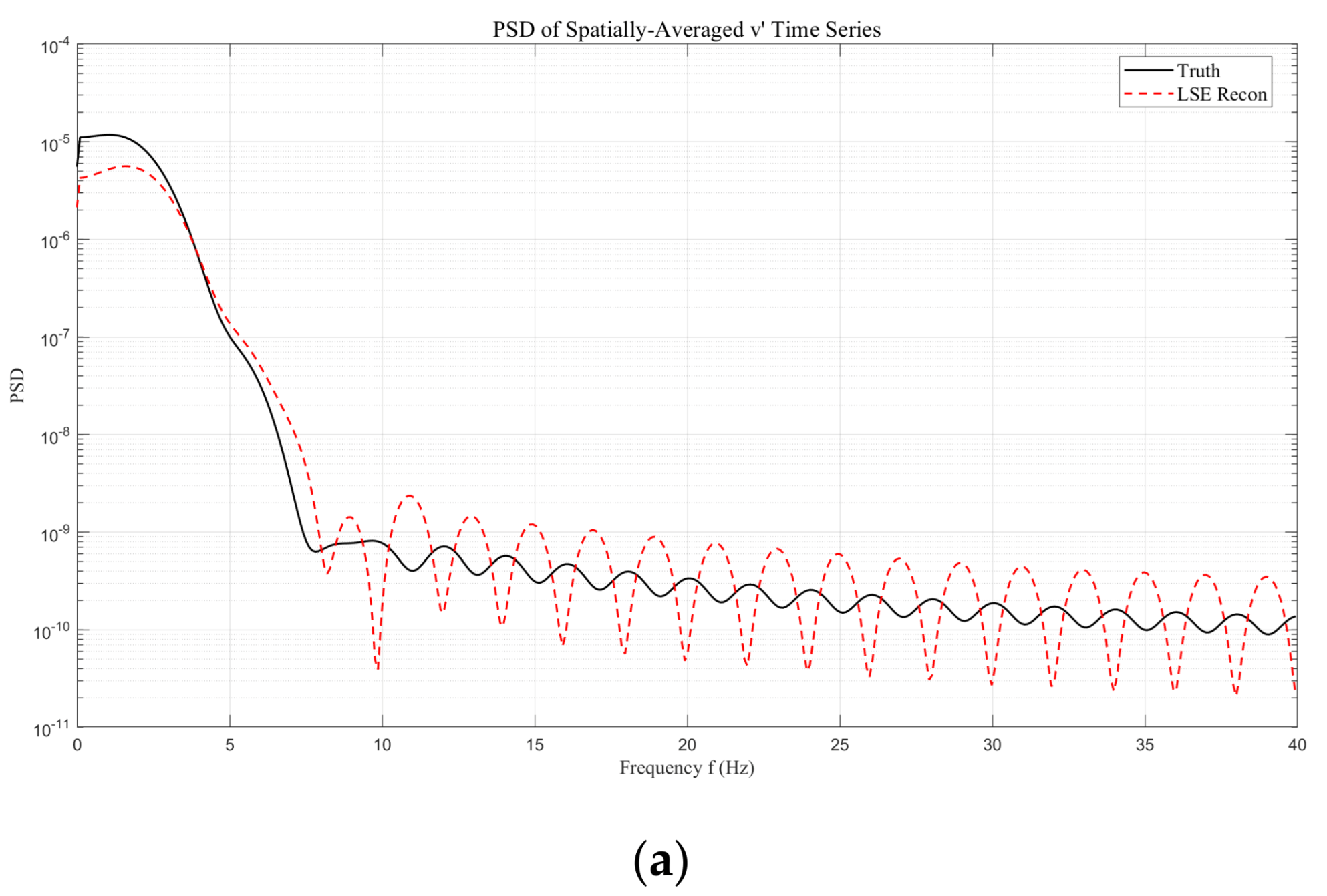
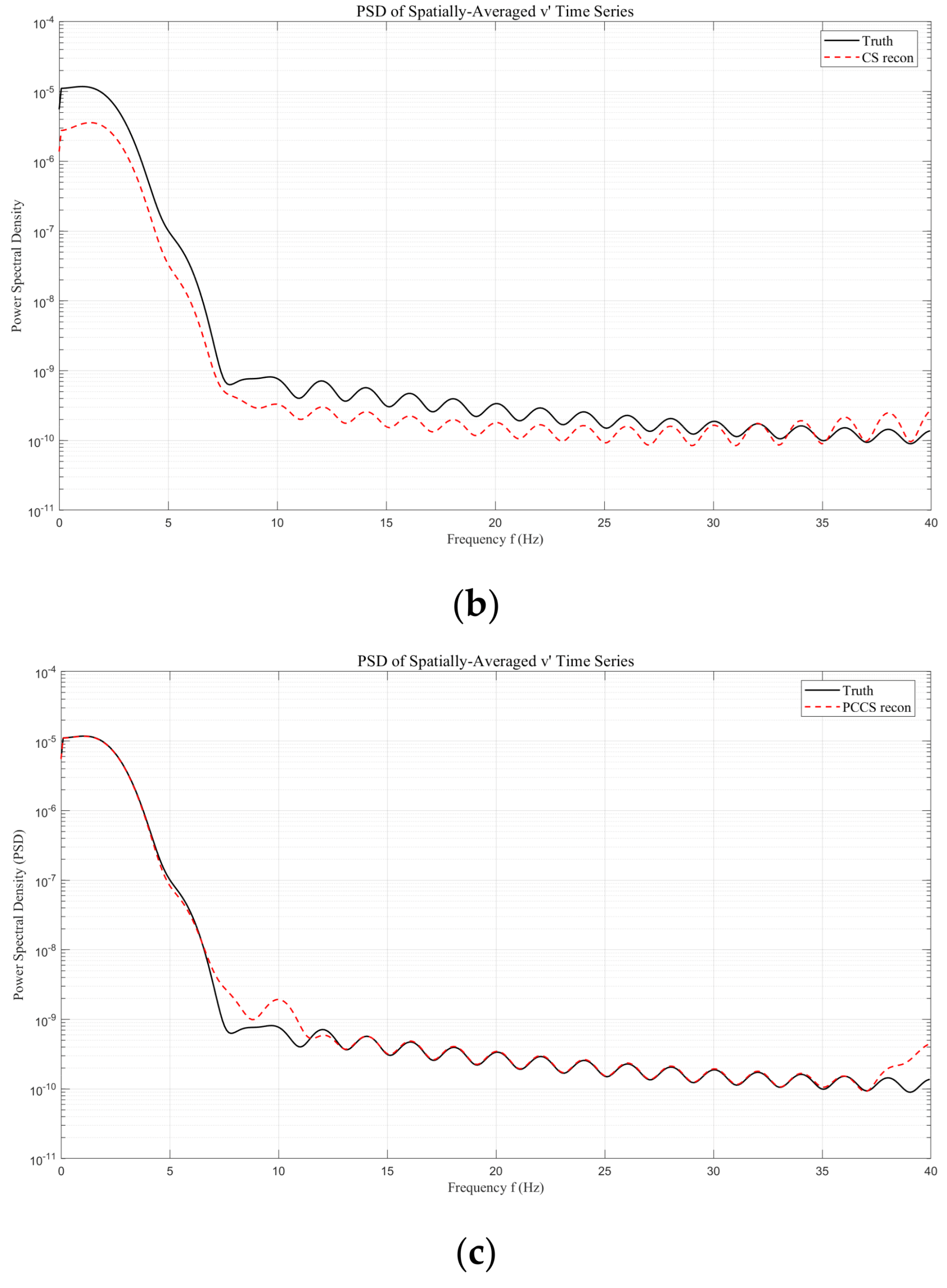
Figure 5 presents the reconstructed power spectral density (PSD) of the spatially averaged velocity fluctuation signal: LSE (Figure 5a): Significantly underestimates high-frequency energy above the shedding peak, causing the PSD curve to drop sharply in the mid-to-high-frequency range. CS (Figure 5b): Recovers more high-frequency components but introduces discrete spurious peaks and nonphysical spectral noise. PCCS (Figure 5c): Maintains excellent agreement with the true spectrum across the entire frequency range, accurately restoring the primary spectral peak amplitude while suppressing the CS-induced high-frequency artefacts. The mean absolute dB error (MADE) for PCCS is computed as only 0.71 dB, compared to 2.59 dB for CS and 3.81 dB for LSE.

In summary, by incorporating point-measurement constraints on high-frequency content, the PCCS method not only fully recovers instantaneous vortex-shedding structures but also achieves substantial improvements over traditional LSE and pure CS in both spatial statistical moments and spectral fidelity, thereby demonstrating its superior capability for reconstructing non-periodic, multi-frequency flows with enhanced spatiotemporal resolution.

3.2. Application to Ccomplex Wake: Tandem Cylinders (Re ≈ 10³)

The measurement matrix corresponds to the sampling algorithm in PIV. POD analysis is first applied to the down sampled 591 snapshots, whose smallest interval between two adjacent snapshots is bigger than 0.25 s. In view of the modes decomposed by POD that are used to accomplish a reconstruction, the average flow field is included in modes. The variance spectrum and POD modes are presented in Figure 6. It is obvious that only the first mode, also meaning the average flow, is the dominating one, which contributes approximately 79% of the total fluctuating energy, as Figure 6a depicted. A sum of 100 modes consume about 98% fluctuating variance and higher-order modes still contribute little energy due to the turbulence in the flow. The first three modes are shown in Figure 6b: the average wake flow is on the left, the second mode in the middle, and the third mode on the right. Vortex structures are concentrated in the wake of big cylinder in captured the second and third modes. In this article, the first 100 modes are employed in the following reconstruction implementation.

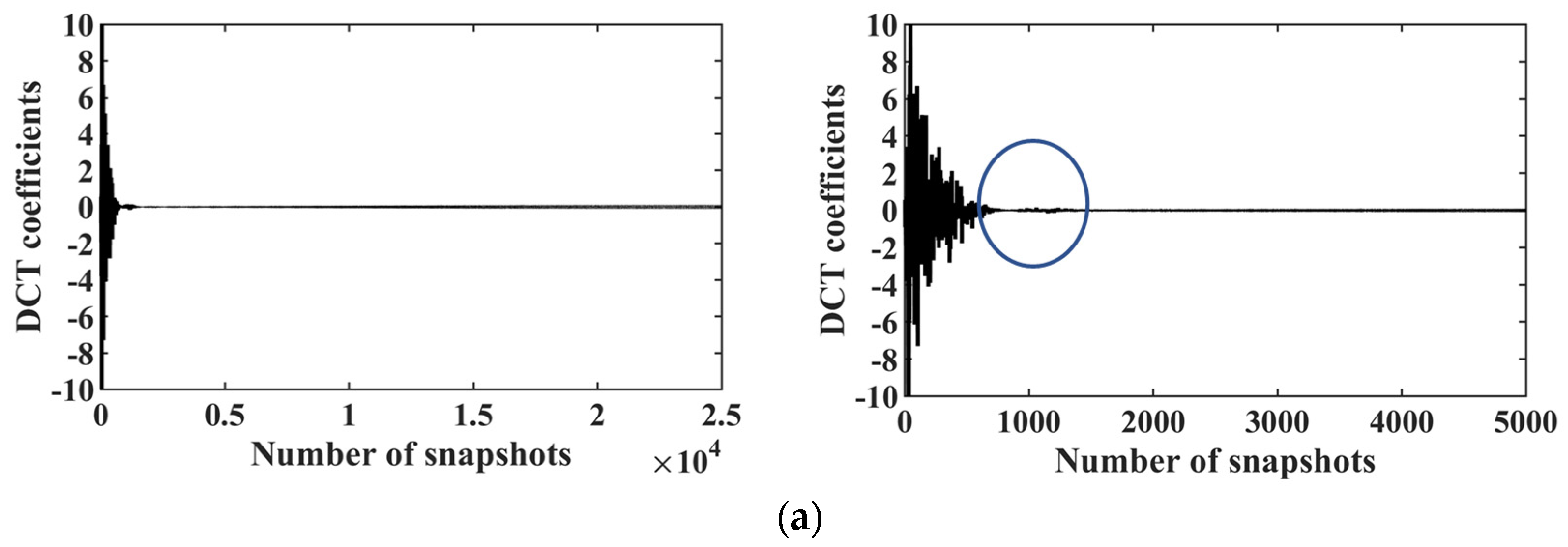
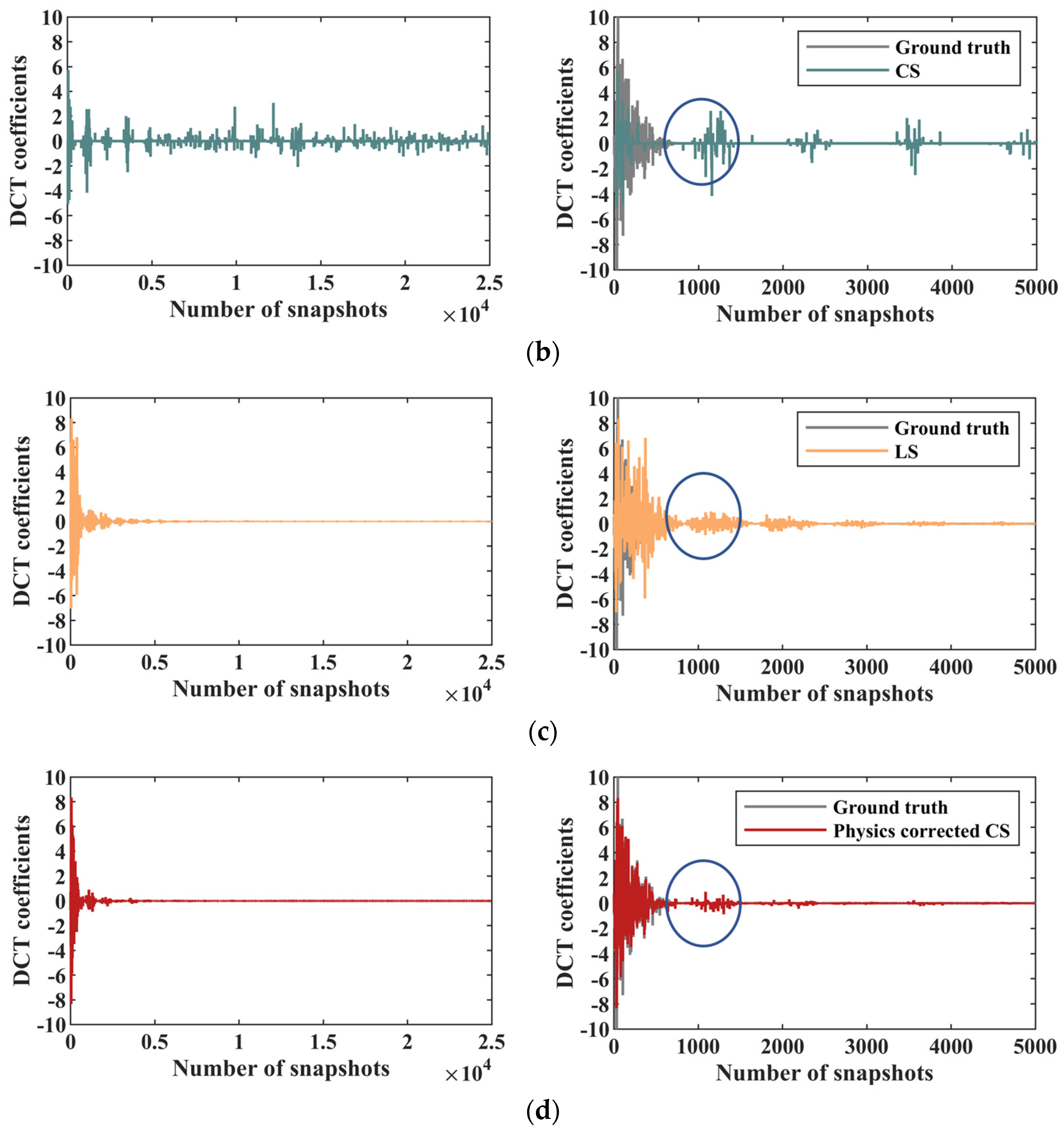
Figure 7 compares the DCT coefficients reconstructed using CS, LS, and data fusion CS methods. The distribution of DCT coefficients across the x-axis reflects the frequency information from lower to higher bands [23]. From the ground truth time-resolved data in Figure 7a, it is obvious that DCT coefficients are sparse, indicating a feasibility using CS reconstruction. However, as shown in Figure 7b, the CS reconstruction from down-sampled PIV data is remarkably deviated from the ground truth values. This phenomenon can be explained by congenital defects of BP algorithm. Though BP algorithm can provide a higher accuracy, $L_1$-norm cannot distinguish the location of the sparse coefficients scale and is thus prone to some artificial effects, namely transfers from low-scale energy to high-scale energy. On the other hand, the LS reconstruction from pointwise time-resolved data, as a $L_2$-norm solution, can remedy the disadvantage in high-frequency noise. However, the LS cannot precisely detect the non-zero values in the DCT spectrum. Therefore, the data fusion method applies LS results as the upper and lower bounds on the DCT coefficients calculated from the CS solution. This approach significantly enhances the accuracy of the DCT coefficients compared to using the CS and LS methods separately.

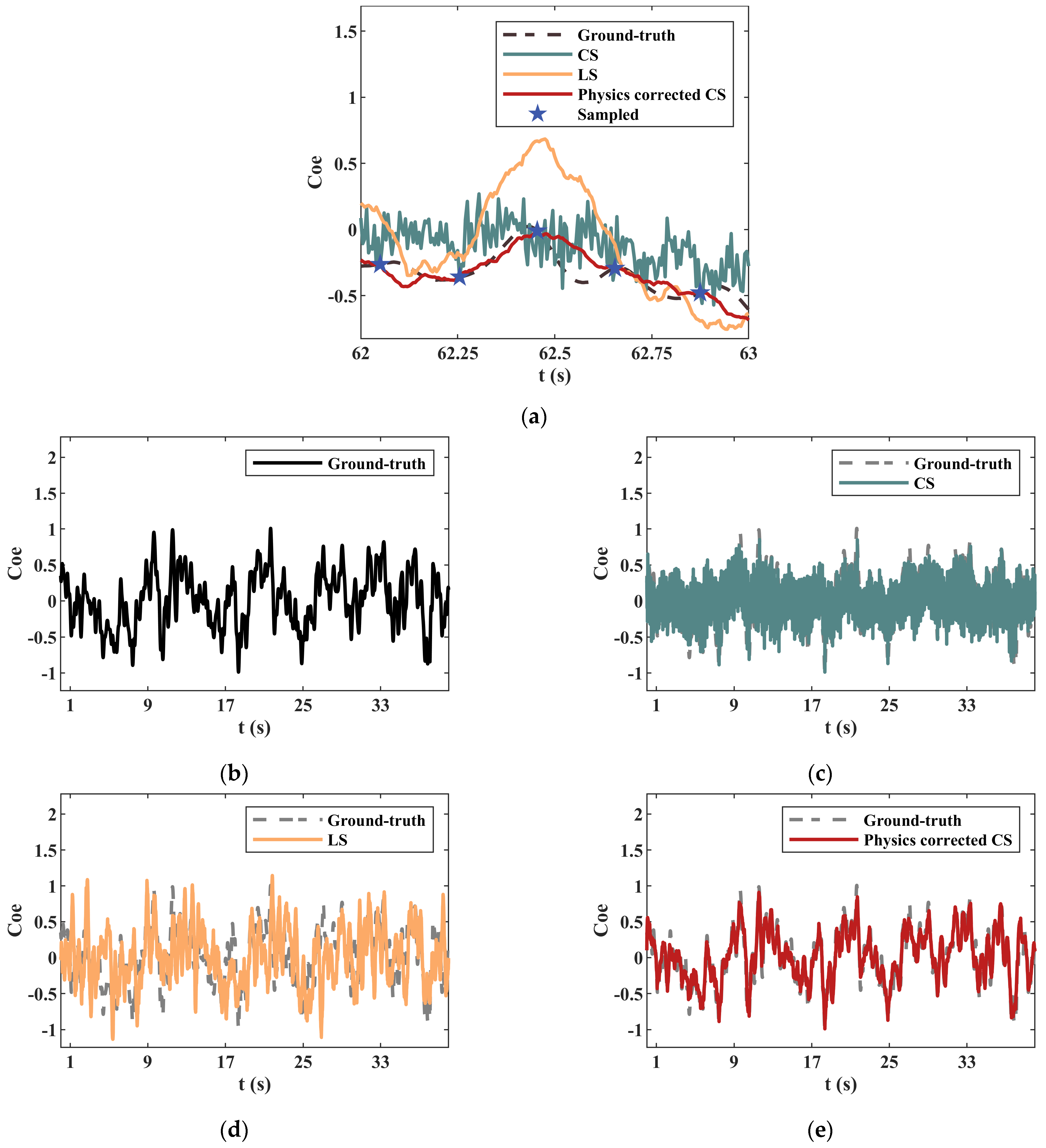
The reconstructed POD coefficients from the DCT spectrum are compared in Figure 8. The temporal resolution is significantly improved. Figure 8a presents the coefficients in short-time period to show the details, whereas Figure 8b-e presents the coefficients in a long-time period. The down-sampled points are marked by the blue stars in Figure 8a. In the short-time period, the CS reconstruction from down-sampled PIV data clearly has strong noise compared to the ground truth. The LS method based on pointwise time-resolved data can depress the noise, but the calculated values deviate from the ground-truth data remarkably. As a contrast, the data fusion CS can more faithfully reconstruct the temporal coefficients with much less noise. The comparison is more obvious for the long-time period, as shown in Figure 8b–e.

However, the reconstructed POD coefficients demonstrated above obey the Nyquist sampling algorithm. POD coefficients corresponding to the fifth mode are an example of sub-sampling and the reconstruction results are shown in the following parts. Likewise, DCT coefficients, as shown in Figure 9, are first given to compare the reconstruction results via CS, LS and PCCS, respectively. The left parts, as showed before, represent the DCT coefficients in long data sequences and the right parts are short data sequences to amplify the non-zero parts. Remarkable deviations for CS from the ground-truth data exist in both high-frequency parts and low-frequency parts, which can also be explained by the artificial effects of $L_1$-norm. LS reconstruction, like before, loses the value accuracy but detects the existence of the frequency variance with a relatively accuracy. The PCCS, as Figure 9d showed, combines the advantages of both CS and LS, overcoming the energy transfer and inaccuracy in low-frequency parts at the same time. However, it is well-known that low-frequency parts contain more information than high-frequency parts for low-frequency parts reflect the outline of signals. Therefore, the inaccuracy is acceptable.

Figure 10 gives a comparison for the reconstructed POD coefficients between ground-truth, CS, LS, and PCCS. The coefficients corresponding to the sampled snapshots are also marked by the blue stars in Figure 10a. In a short time series, it is obvious that there exists a great deal of high-frequency fluctuations for CS reconstruction, as indicated by Figure 7a. In addition, the reconstructed values seem higher than the ground-truth data on the whole. The reconstructed POD coefficients by LS regression, however, deviates from the ground-truth data remarkably, which is in accordance with the result of DCT coefficients. As a contrast, PCCS reconstruction has only very slight fluctuations around the ground-truth data and has an accurate outline fitting the ground-truth curve. In a longer time series, the reconstruction performance is clearer, as shown in Figure 10b–e. Characterizing a fuzzy outline of the ground-truth data, CS reconstruction seems provide an approximation to real coefficients, presenting a similar result as the reconstructed data before. Too many high-frequency fluctuations around real data are unable to be neglected, which indicates a low reconstruction accuracy. The LS reconstructed data, like before, lose the essential features of the original data. As a sharp contrast, PCCS provides an almost perfect approximation in a manner of speaking.

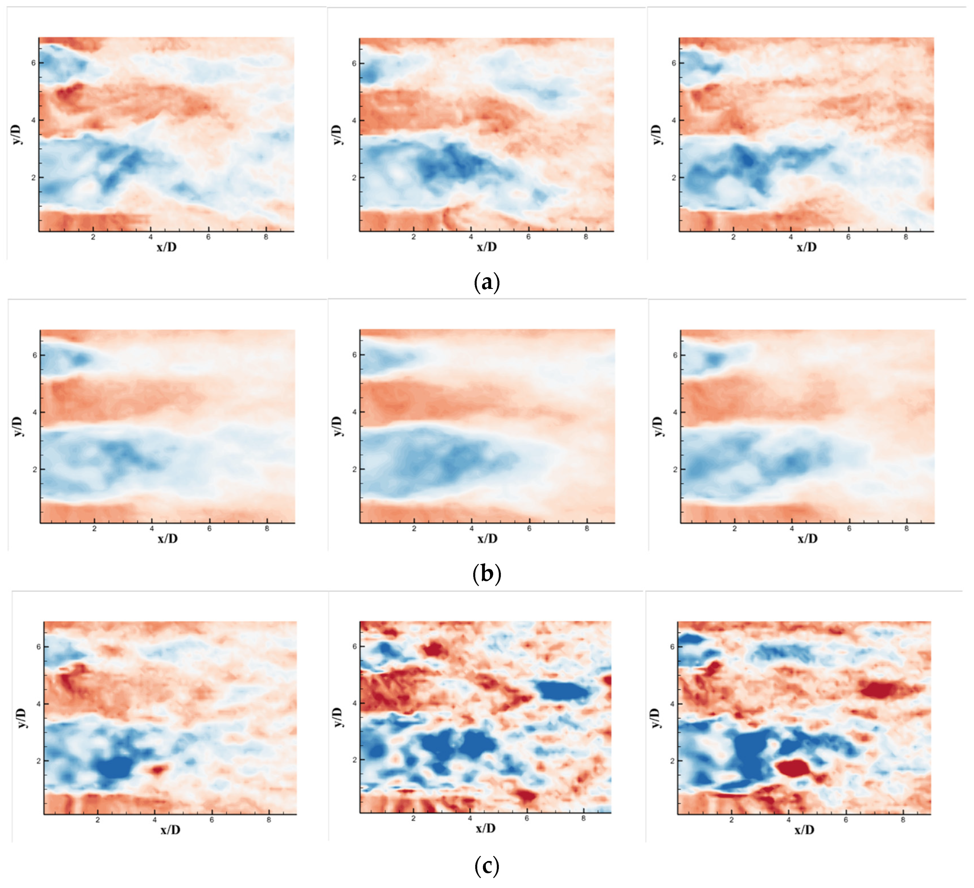
Based on the reconstructed POD coefficients, the time-resolved flow field snapshots are obtained and compared with the ground truth in Figure 11. Figure 11 compares representative reconstructed flow field snapshots against the ground truth. Notably, the snapshots shown are taken at times that were not directly captured by PIV (i.e., intermediate time steps), demonstrating the PCCS method’s ability to produce high-temporal-resolution flow fields beyond the original sampling instants. Consistent with the frequency-domain findings, the CS-only reconstruction captures the overall wake pattern but fails to reproduce finer spatial details due to spurious high-frequency noise. The LS-only reconstruction is even worse, yielding unphysical, discrete flow features because the very limited pointwise data cannot represent the continuous spatial structures or the overall trend of the flow. In contrast, the PCCS reconstruction preserves both the global flow pattern and the local flow details with high fidelity, producing snapshots whose vortex structures and velocity magnitudes closely match the ground truth. This highlights the method’s superior spatial and temporal reconstruction accuracy compared to the other approaches.

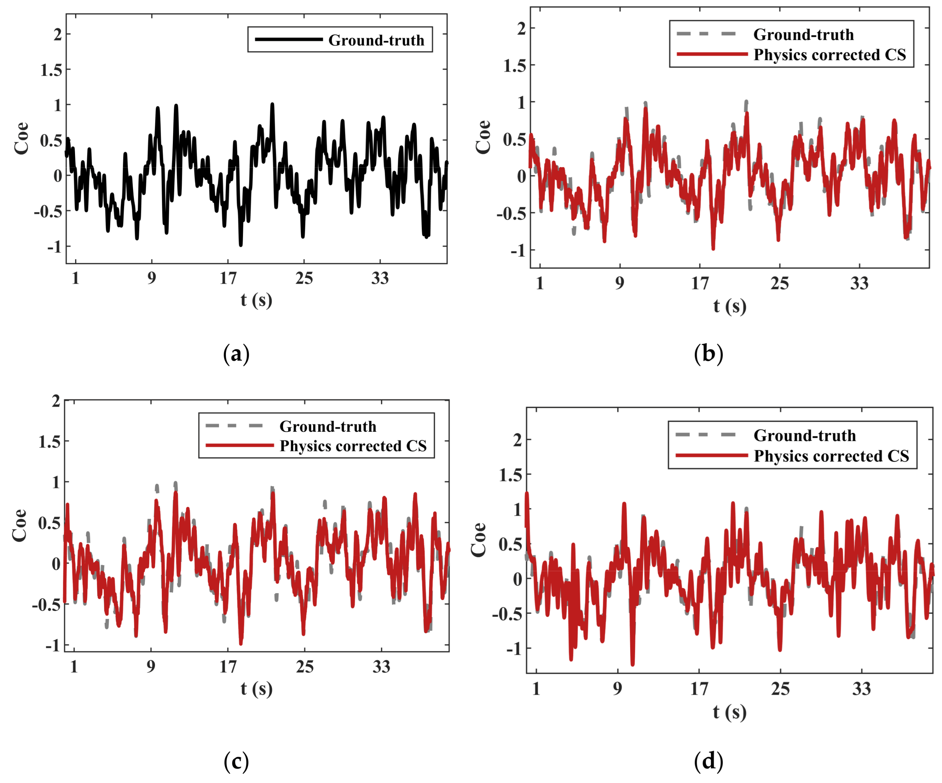
The number of probes is then reduced to compare the reconstruction performance, as depicted in Figure 12, which is described in a long time series corresponding to mode 5. Figure 10a–d corresponds to employing seven probes, four probes and two probes, respectively. It is clear that the fitting becomes poorer when the number of probes is reduced gradually, appearing as more high-frequency noise and error values. However, though the reconstruction performance when employing two probes turns down compared to employing seven probes, PCCS is still a strong performer compared to CS and LS, as shown in Figure 10c,d.

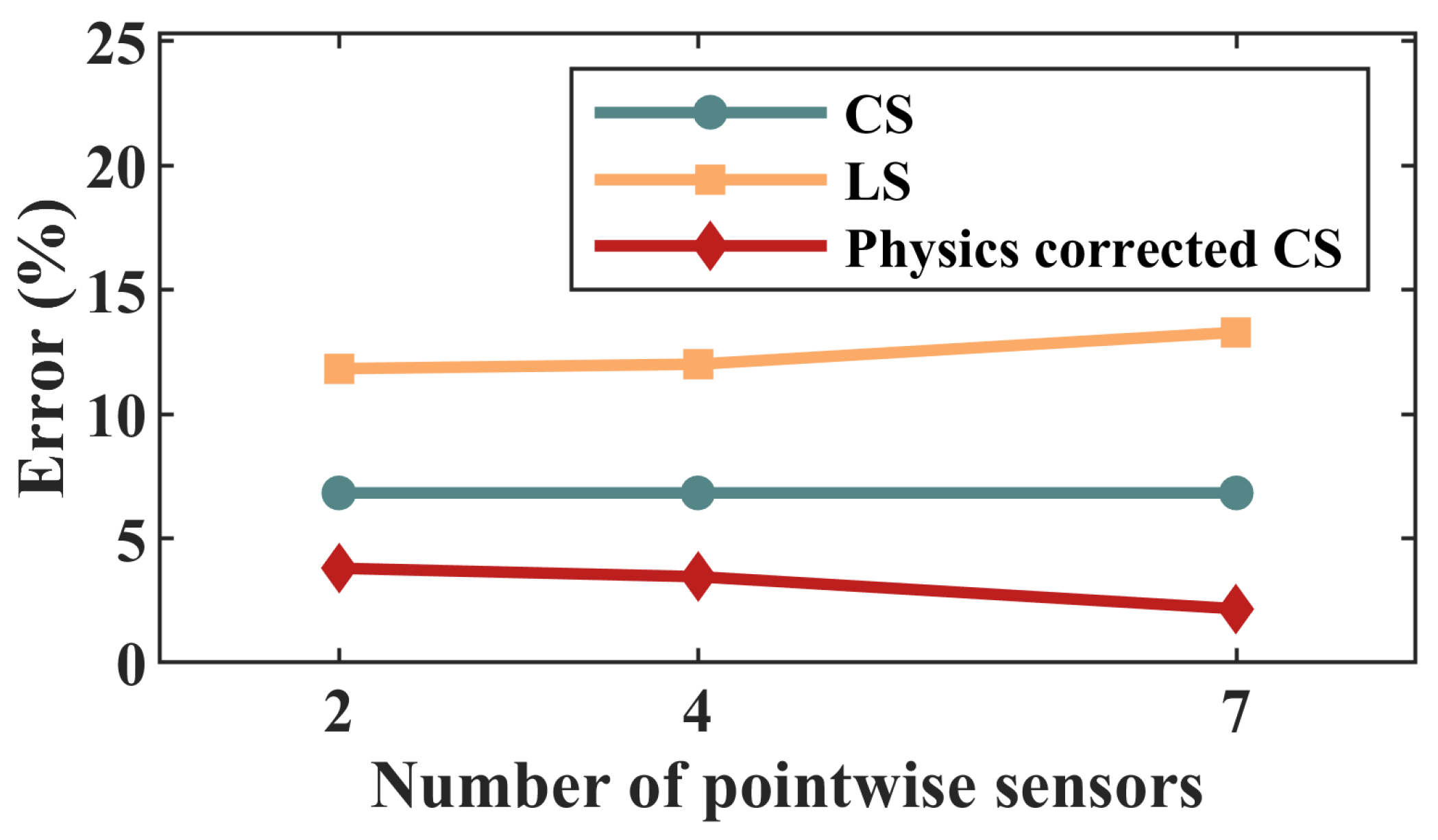
To precisely illustrate the accuracy of the reconstructed data, the error, defined by comparing the recovered and ground-truth data, was calculated using the following relation prescribed by Ruscher et al. [24], as follows:

$$e_i={\displaystyle \frac{{|u}_i^{recon}-u_i^{truth}|}{u_{max}^{truth}-u_{min}^{truth}}}\mathrm{\%}$$

(12)

where $u_i^{recon}$ represents the reconstructed velocity at spatial location $i$, while $u_i^{truth}$ denotes the corresponding ground-truth velocity. The variables $u_{max}^{truth}$ and $u_{min}^{truth}$ denote maximum and minimum values in whole 25,000 snapshots, respectively, across the entire region. The error for every snapshot is then calculated by averaging the errors in all locations and the final error shown in Figure 13 is the average value for all the reconstructed snapshots avoiding the sampled data. It is noted that the probes are not required in CS reconstruction while both LS and PCCS need to employ pointwise sensors. In order to give an intuitive error contrast, CS reconstruction error is figured on the same picture. Obviously, no matter employing two probes or four probes or seven probes, PCCS reconstruction has a higher accuracy than CS reconstruction and LS reconstruction. With the number of sensors increasing, PCCS reconstruction has a better performance while LS is on the contrary.

The study additionally computes the power-spectral density (PSD) and defines the mean absolute deviation in energy (MADE) in decibel units. Furthermore, the global L₂-norm errors between the reconstructed and reference fields are evaluated for the first-, second-, and third-order moments—mean, variance, and skewness—to provide a more comprehensive quantification of each method’s ability to capture the multi-frequency, aperiodic characteristics of the flow

Table 2. Accuracy metrics for LSE, CS, and PCCS reconstructions: percentage errors in the 1st, 2^nd, and 3rd statistical moments.

Method	Error1	Error2	Error3
LSE	23.67%	89.44%	98.22%
CS	6.87%	58.96%	67.37%
PCCS	2.60%	26.66%	45.39%

summarizes the percentage errors of the three methods for the first-, second-, and third-order moments. PCCS attains the lowest errors, 2.6%, 26.66%, and 45.39%, respectively, markedly outperforming both CS and LSE.

In Figure 14, the power-spectral–density (PSD) curves of the spatially averaged fluctuating-velocity signal are compared. As shown in Figure 14a, the LSE method satisfactorily reconstructs the large-scale, low-frequency structures yet fails to recover the high-frequency turbulent content. The CS approach (Figure 14b) reproduces the dominant frequency reasonably well but cannot suppress the spurious high-frequency components. By contrast, the PCCS solution (Figure 14c) aligns almost perfectly with the DNS reference over the entire spectral range, accurately capturing the principal vortex-shedding frequency while effectively eliminating the high-frequency artefacts introduced by CS. In terms of the mean absolute deviation in energy (MADE), LSE yields 7.9 dB and CS suffers from large errors in the high-frequency band, whereas PCCS records only 0.9 dB, exhibiting markedly higher accuracy than both LSE and CS.

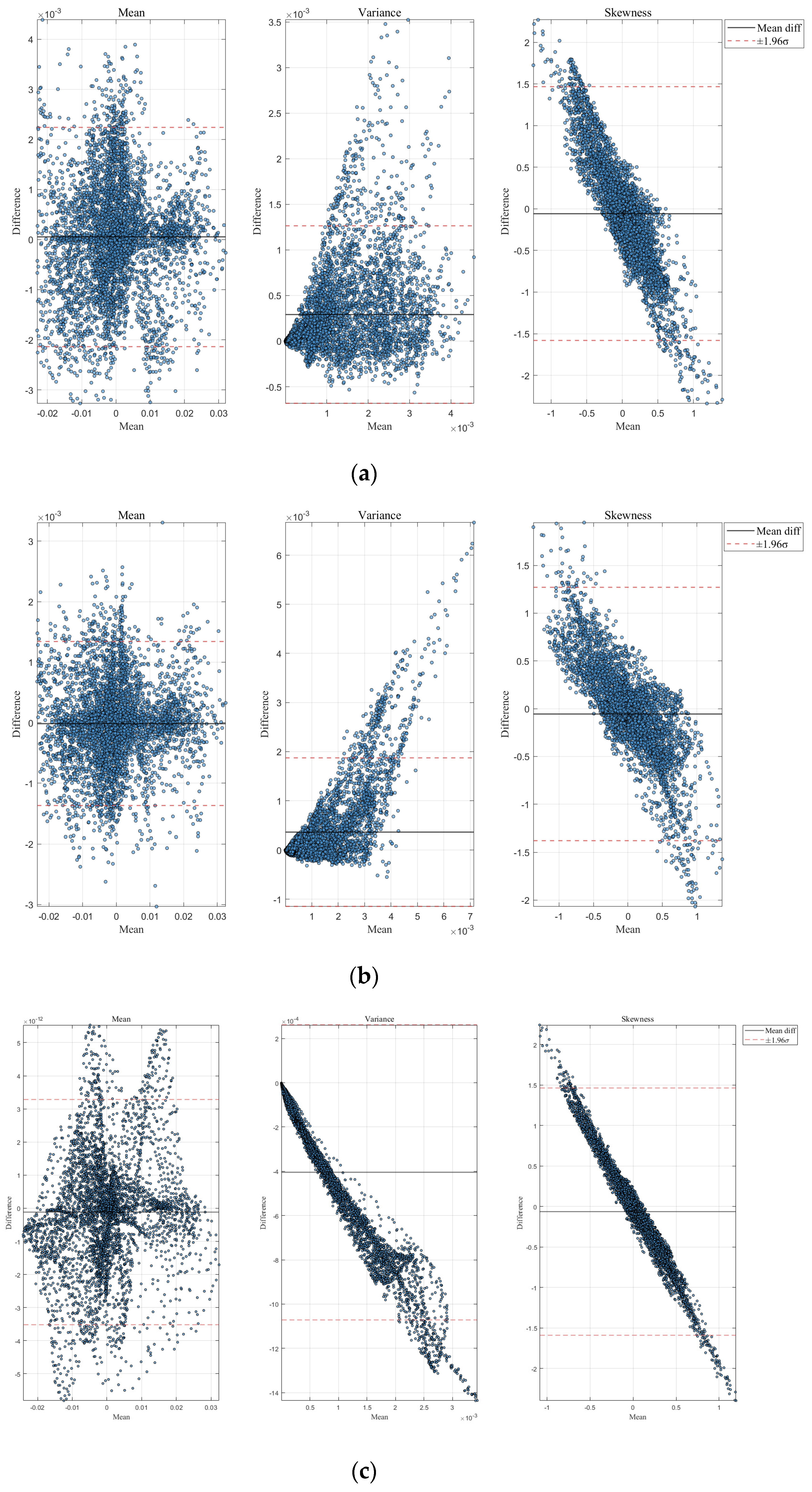
Figure 15 compares the spatial distributions of the relative errors in the first- (mean), second- (variance), and third-order (skewness) moments obtained with the three reconstruction techniques.

As illustrated in Figure 15a, the LSE approach displays a markedly higher relative error, revealing its inability to capture small-scale, high-frequency features during reconstruction. By contrast, the CS method (Figure 15b) lowers the overall error substantially, indicating that the sparsity-promoting strategy effectively suppresses global discrepancies, although localized peaks remain evident. The PCCS technique (Figure 15c) produces a dense cluster of points confined to a narrow band around the zero-difference line and exhibits the tightest confidence limits, demonstrating well-controlled errors. These observations collectively substantiate the superiority of PCCS in recovering the spatiotemporal resolution of the flow field.

4. Conclusions and Discussions

This article proposes a high-temporally resolved data reconstruction method termed Physics Corrected Compressive Sensing (PCCS). This approach integrates measurements from particle image velocimetry (PIV), which have high spatial resolution but low temporal resolution, with a few pointwise probes that offer high temporal resolution but low spatial resolution. By combining these complementary data sources, PCCS yields flow field reconstructions that retain the fine spatial details of the PIV measurements while achieving the high temporal resolution of the pointwise probe data, effectively overcoming the resolution trade-off of each individual technique.

In the proposed PCCS reconstruction, proper orthogonal decomposition (POD) is initially applied to the low-temporally-resolved PIV data to obtain spatial POD modes and the corresponding low-frequency temporal coefficients. These modes are then combined with the point-sensor time series via least-squares regression to obtain high-temporally resolved POD coefficients. The high-temporal-resolution POD coefficients are subsequently transformed into the sparse reciprocal space via a discrete cosine transform (DCT). The DCT coefficients from the pointwise regression serve as upper and lower bounds on the CS solution, adding physical constraints to the pure data-driven CS problem. The measurement matrix corresponds to the PIV sampling pattern, and the DCT acts as the sparse transform. In summary, PCCS introduces physics-based bounds into compressive sensing to stabilize the solution and suppress spurious high-frequency content.

The performance of the PCCS method was evaluated using a non-periodic, multi-frequency wake flow behind two cylinders. The results show that the standard CS reconstruction (using only PIV data) yields a time-averaged error of about 6.8%, and the LS reconstruction (using only point probe data) yields about 13% error, whereas the proposed PCCS method achieves an error of only 2.1% when seven probes are used. In other words, PCCS recovers the flow field with roughly a three-fold reduction in error relative to CS and about one-sixth the error of LS, demonstrating a significant improvement in reconstruction accuracy. Furthermore, we investigated the method’s robustness to fewer point sensors: even with only two probes (instead of seven), PCCS maintains a low reconstruction error (3.7%) that remains superior to the CS and LS approaches. (By comparison, CS does not use probes, and LS cannot operate with less than one probe). This trend shows that as the number of probes increases, PCCS performance further improves (error dropping from 3.7% at two probes to 2.1% at seven probes), whereas the accuracy of the pure LS method actually degrades when more probes are used (due to over-fitting noise). Overall, PCCS consistently outperforms the other methods across all tested sensor counts, indicating its robustness and effectiveness even when pointwise data are limited.

These findings highlight how the incorporation of physical constraints in PCCS leads to superior reconstruction fidelity, as evidenced by the spectral and modal analyses. In the frequency domain, the DCT coefficient spectra (e.g., Figure 7 and Figure 9) show that the PCCS method accurately captures the significant temporal frequencies of the flow without introducing the spurious high-frequency energy observed in the pure CS reconstruction. At the same time, PCCS preserves the correct magnitude of low-frequency components, unlike the pure LS approach, which cannot reproduce the true amplitude distribution of the spectrum. Capturing the correct spectrum is crucial because it ensures that the time evolution of the flow is reconstructed with the proper balance of high- and low-frequency dynamics.

This advantage is reflected in the time-domain POD coefficients: for a dominant low-frequency mode (Figure 8) as well as a higher-frequency, lower-energy mode (mode 5 in Figure 10), the PCCS-reconstructed coefficients closely follow the ground-truth curves with only minimal deviation. In contrast, the CS results exhibit excessively high-frequency oscillations around the true signal, and the LS results show large biases and loss of important fluctuations, especially for the higher modes. The ability of PCCS to recover even higher-order POD modes with high accuracy means that subtle flow features and smaller-scale dynamics (which contribute less energy individually but are important for fidelity) are not lost in the reconstruction. Visual comparisons of reconstructed flow fields confirm these quantitative findings: the PCCS method produces flow snapshots that are nearly indistinguishable from the ground truth in both large-scale structure and fine details (as seen in Figure 11), whereas the CS and LS reconstructions deviate either by adding artificial small-scale noise (CS) or by smoothing out and distorting flow features (LS). In summary, by leveraging PIV’s high spatial resolution and the probes’ high temporal resolution, the PCCS method achieves a high-fidelity reconstruction of the flow in both space and time, dramatically improving upon traditional compressive sensing in this multi-frequency, non-periodic flow scenario.

Furthermore, the spectral and statistical-moment analysis of the single-cylinder benchmark case (Re = 100) shows that PCCS achieves an average absolute dB error (MADE) in the frequency domain of only 0.71 dB—far better than CS (2.59 dB) and LSE (3.81 dB); at the same time, the full-field first-, second-, and third-order moment errors are merely 0.60%, 1.78%, and 29.73%, respectively, significantly outperforming both CS and LSE. This demonstrates that PCCS can accurately recover the principal frequency components and higher-order statistical characteristics of the flow field. For the tandem double-cylinder complex wake (Re ≈ 10³), as shown in Figure 14 and Figure 15 and Table 2, PCCS delivers markedly lower MADE in the PSD reconstruction and substantially reduced first-, second-, and third-order moment errors compared to the other methods, further confirming its robustness and high-fidelity performance in preserving spatial detail and temporal resolution in non-periodic, multi-frequency, broad-spectrum complex flows.

References

1. Druault, P.; Guibert, P.; Alizon, F. Use of Proper Orthogonal Decomposition for Time Interpolation from PIV Data: Application to the Cycle-to-Cycle Variation Analysis of in-Cylinder Engine Flows. Exp. Fluids 2005, 39, 1009–1023. [Google Scholar] [CrossRef]
2. He, C.; Liu, Y. Time-Resolved Reconstruction of Turbulent Flows Using Linear Stochastic Estimation and Sequential Data Assimilation. Phys. Fluids 2020, 32, 075106. [Google Scholar] [CrossRef]
3. Jin, X.; Laima, S.; Chen, W.L.; Li, H. Time-Resolved Reconstruction of Flow Field around a Circular Cylinder by Recurrent Neural Networks Based on Non-Time-Resolved Particle Image Velocimetry Measurements. Exp. Fluids 2020, 61, 1–23. [Google Scholar] [CrossRef]
4. Donoho, D.L. Compressed Sensing. IEEE Trans. Inf. Theory 2006, 52, 1289–1306. [Google Scholar] [CrossRef]
5. Candès, E.J.; Romberg, J.; Tao, T. Robust Uncertainty Principles: Exact Signal Reconstruction from Highly Incomplete Frequency Information. IEEE Trans. Inf. Theory 2006, 52, 489–509. [Google Scholar] [CrossRef]
6. Candes, E.J.; Tao, T. Decoding by Linear Programming. IEEE Trans. Inf. Theory 2005, 51, 4203–4215. [Google Scholar] [CrossRef]
7. Huang, X. Compressive Sensing and Reconstruction in Measurements with an Aerospace Application. AIAA J. 2013, 51, 1011–1016. [Google Scholar] [CrossRef]
8. Bai, Z.; Wimalajeewa, T.; Berger, Z.; Wang, G.; Glauser, M.; Varshney, P.K. Low-Dimensional Approach for Reconstruction of Airfoil Data via Compressive Sensing. AIAA J. 2015, 53, 920–933. [Google Scholar] [CrossRef]
9. Bourguignon, J.L.; Tropp, J.A.; Sharma, A.S.; McKeon, B.J. Compact Representation of Wall-Bounded Turbulence Using Compressive Sampling. Phys. Fluids 2014, 26, 015109. [Google Scholar] [CrossRef]
10. Tu, J.H.; Rowley, C.W.; Kutz, J.N.; Shang, J.K. Spectral Analysis of Fluid Flows Using Sub-Nyquist-Rate PIV Data. Exp. Fluids 2014, 55, 1–13. [Google Scholar] [CrossRef]
11. Chen, G.H.; Tang, J.; Leng, S. Prior Image Constrained Compressed Sensing (PICCS): A Method to Accurately Reconstruct Dynamic CT Images from Highly Undersampled Projection Data Sets. Med Phys. 2008, 35, 660–663. [Google Scholar] [CrossRef]
12. Chen, G.-H.; Tang, J.; Leng, S. Prior Image Constrained Compressed Sensing (PICCS). In Photons Plus Ultrasound: Imaging and Sensing 2008: The Ninth Conference on Biomedical Thermoacoustics, Optoacoustics, and Acousto-Optics; SPIE: Bellingham, WA, USA, 2008; Volume 6856, p. 685618. [Google Scholar] [CrossRef]
13. Lu, Y.; Wang, Y. Monitoring Temperature in Additive Manufacturing with Physics-Based Compressive Sensing. J. Manuf. Syst. 2018, 48, 60–70. [Google Scholar] [CrossRef]
14. Lu, Y.; Wang, Y. An Efficient Transient Temperature Monitoring of Fused Filament Fabrication Process with Physics-Based Compressive Sensing. IISE Trans. 2018, 51, 168–180. [Google Scholar] [CrossRef]
15. Lu, Y.; Wang, Y. Physics-Based Compressive Sensing Approach to Monitor Turbulent Flow. AIAA J. 2020, 58, 3299–3307. [Google Scholar] [CrossRef]
16. Liang, Y.C.; Lee, H.P.; Lim, S.P.; Lin, W.Z.; Lee, K.H.; Wu, C.G. Proper Orthogonal Decomposition and Its Applications—Part I: Theory. J. Sound Vib. 2002, 252, 527–544. [Google Scholar] [CrossRef]
17. Sirovich, L.; Kirby, M. Low-Dimensional Procedure for the Characterization of Human Faces. J. Opt. Soc. Am. A 1987, 4, 519–524. [Google Scholar] [CrossRef]
18. He, C.; Liu, Y. Proper Orthogonal Decomposition-Based Spatial Refinement of TR-PIV Realizations Using High-Resolution Non-TR-PIV Measurements. Exp. Fluids 2017, 58, 1–22. [Google Scholar] [CrossRef]
19. Wen, X.; Li, Z.; Peng, D.; Zhou, W.; Liu, Y. Missing Data Recovery Using Data Fusion of Incomplete Complementary Data Sets: A Particle Image Velocimetry Application. Phys. Fluids 2019, 31, 025105. [Google Scholar] [CrossRef]
20. Taira, K.; Colonius, T. The immersed boundary method: A projection approach. J. Comput. Phys. 2007, 225, 2118–2137. [Google Scholar] [CrossRef]
21. Wang, S.; Liu, Y. Wake Dynamics behind a Seal-Vibrissa-Shaped Cylinder: A Comparative Study by Time-Resolved Particle Velocimetry Measurements. Exp. Fluids 2016, 57, 1–20. [Google Scholar] [CrossRef]
22. Zhang, Q.; Liu, Y.; Wang, S. The Identification of Coherent Structures Using Proper Orthogonal Decomposition and Dynamic Mode Decomposition. J. Fluids Struct. 2014, 49, 53–72. [Google Scholar] [CrossRef]
23. Oppenheim, A.V.; Schafer, R.W.; Buck, J.R. Discrete-Time Signal Processing, 2nd ed.; Prentice-Hall, Inc.: Upper Saddle River, NJ, USA, 1999. [Google Scholar]
24. Ruscher, C.J.; Dannenhoffer, J.F.; Glauser, M.N. Repairing Occluded Data for a Mach 0.6 Jet via Data Fusion. AIAA J. 2017, 55, 255–264. [Google Scholar] [CrossRef]
Figure 1. Schematic of the data fusion CS reconstruction approach.
Fluids 10 00192 g001
Figure 2. Schematic of measurements: (a) PIV measurement regions; (b) pointwise measurement locations.
Fluids 10 00192 g002
Figure 3. Comparison of instantaneous cross-stream velocity reconstructed by different methods: (a) LSE; (b) CS; (c) PCCS for the single-cylinder wake (Re = 100, circles denote probe locations).
Fluids 10 00192 g003
Figure 4. Spatial distribution of reconstruction errors in the first-, second-, and third-order velocity moments obtained by three methods: (a) LSE; (b) CS; (c) PCCS for the single-cylinder wake (Re = 100).
Fluids 10 00192 g004
Figure 5. PSD of the spatially averaged fluctuating velocity obtained by three different methods: (a) LSE; (b) CS; (c) PCCS.
Fluids 10 00192 g005aFluids 10 00192 g005b
Figure 6. POD analysis: (a) energy spectrum of POD modes; (b) first 3 POD modes.
Fluids 10 00192 g006
Figure 7. DCT coefficients corresponding to mode 1 of long range (left) and short range (right): (a) ground-truth coefficients; DCT coefficients of reconstructed POD coefficients by: (b) CS (c) LS (d) PCCS.
Fluids 10 00192 g007aFluids 10 00192 g007b
Figure 8. Comparison of POD coefficients corresponding to mode 1: (a) comparison for different reconstruction methods in short range; Different reconstruction methods in long range: (b) ground-truth; (c) CS; (d) LS; (e) PCCS.
Fluids 10 00192 g008
Figure 9. DCT coefficients corresponding to mode 1 of long range (left) and short range (right): (a) ground-truth coefficients; DCT coefficients of reconstructed POD coefficients by (b) CS; (c) LS; (d) PCCS.
Fluids 10 00192 g009
Figure 10. POD coefficients corresponding to mode 5: (a) comparison for different reconstruction methods in short range; different reconstruction methods in long range: (b) ground-truth; (c) CS; (d) LS (e) PCCS.
Fluids 10 00192 g010
Figure 11. Reconstructed snapshots: (a) ground-truth; (b) CS; (c) LS; (d) PCCS.
Fluids 10 00192 g011aFluids 10 00192 g011b
Figure 12. Reconstructed POD coefficients employing 2 probes: (a) ground-truth; (b) CS; (c) LS; (d) PCCS.
Fluids 10 00192 g012
Figure 13. Error incurred in data recovery vs. the number of pointwise sensors employed in reconstruction.
Fluids 10 00192 g013
Figure 14. PSD of the spatially averaged fluctuating velocity obtained by three different methods: (a) LSE; (b) CS; (c) PCCS.
Fluids 10 00192 g014
Figure 15. Bland–Altman analysis of reconstructed velocity-field statistics using three algorithms: (a) LSE; (b) CS; (c) PCCS.
Fluids 10 00192 g015