


Assessing the Effect of Air Ventilation on the Dispersion of Exhaled Aerosol Particles in a Lecture Hall: Simulation Strategy and Streamlined Workflow

Abstract
1. Introduction
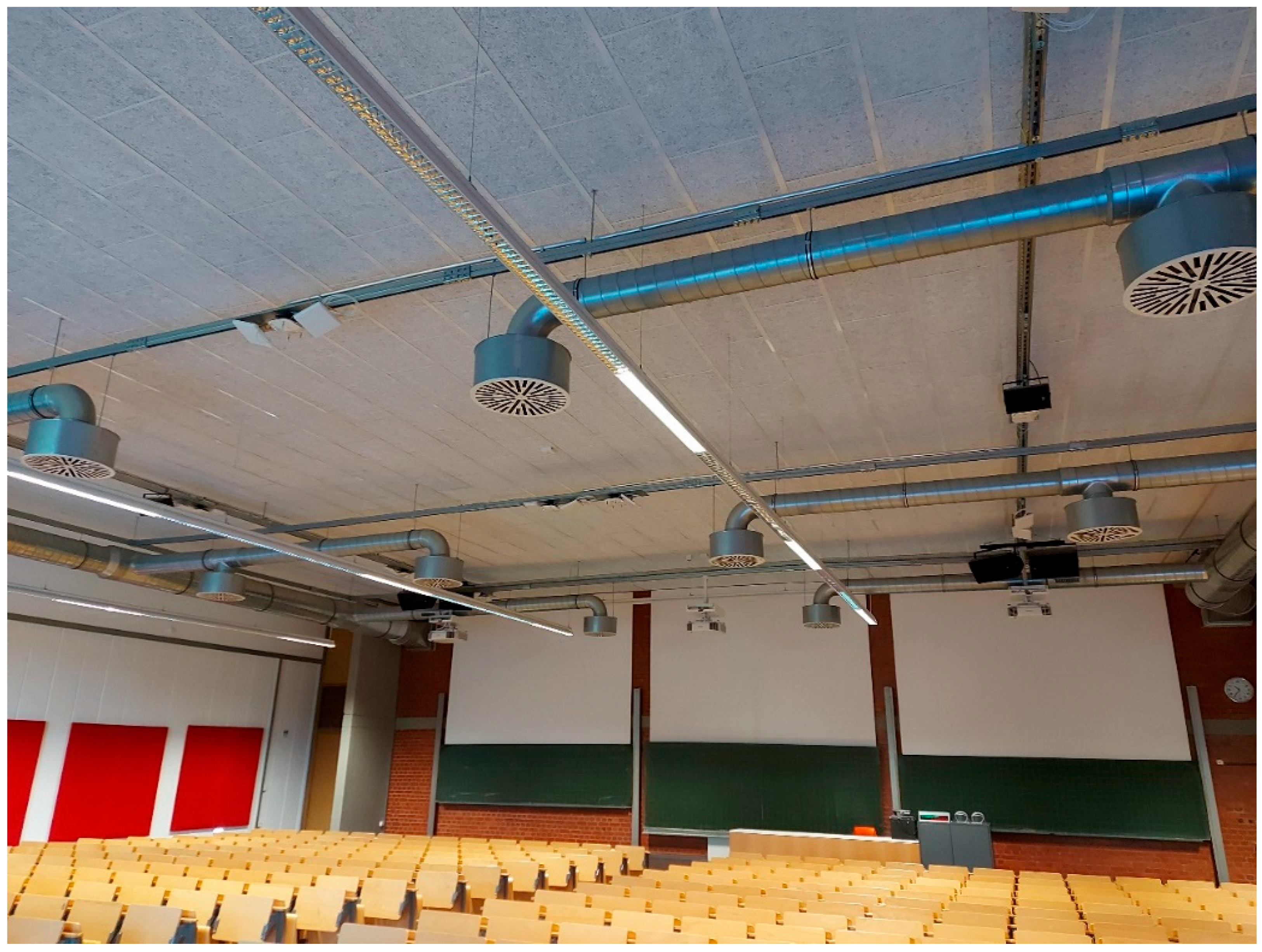
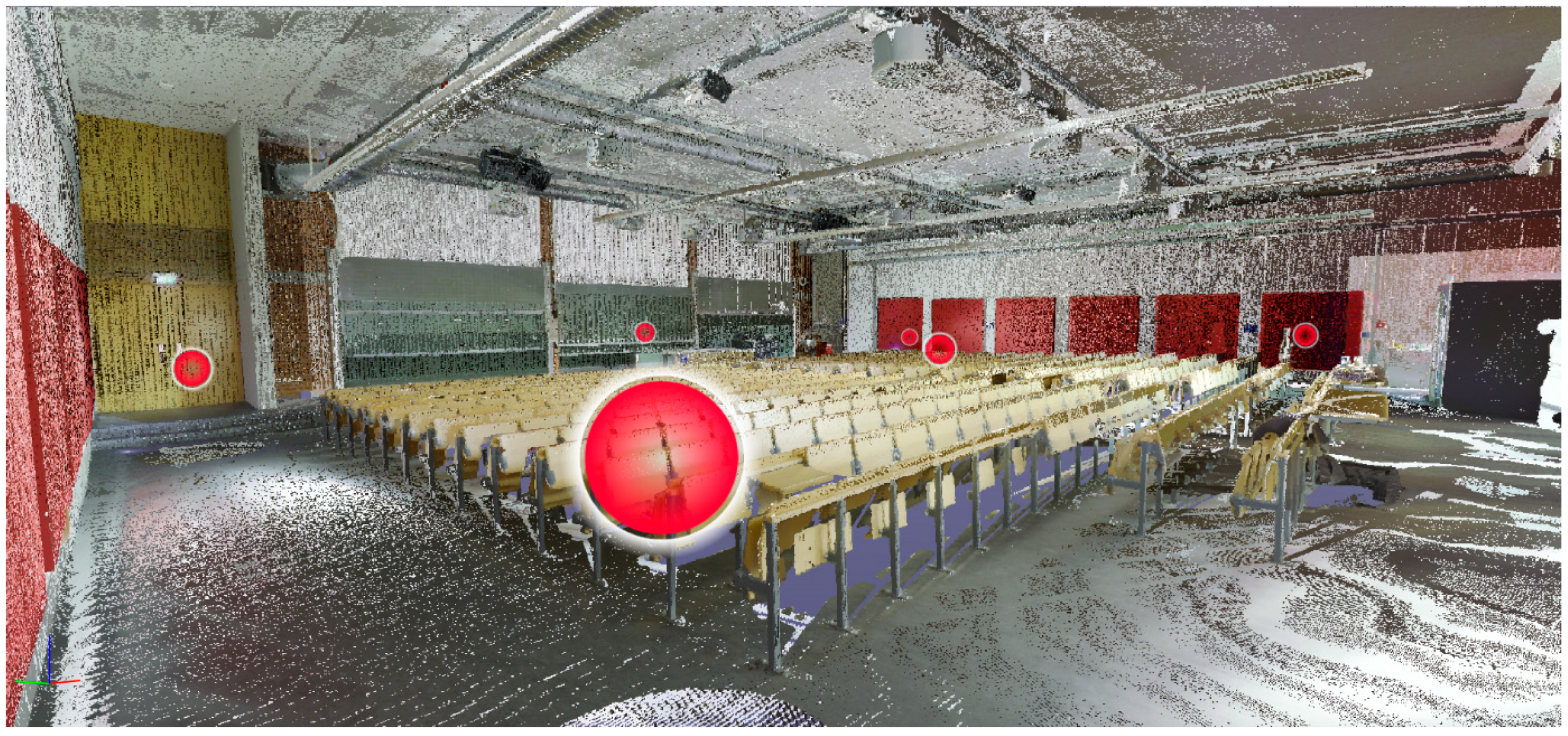
2. Room and Venting System—Data Collection
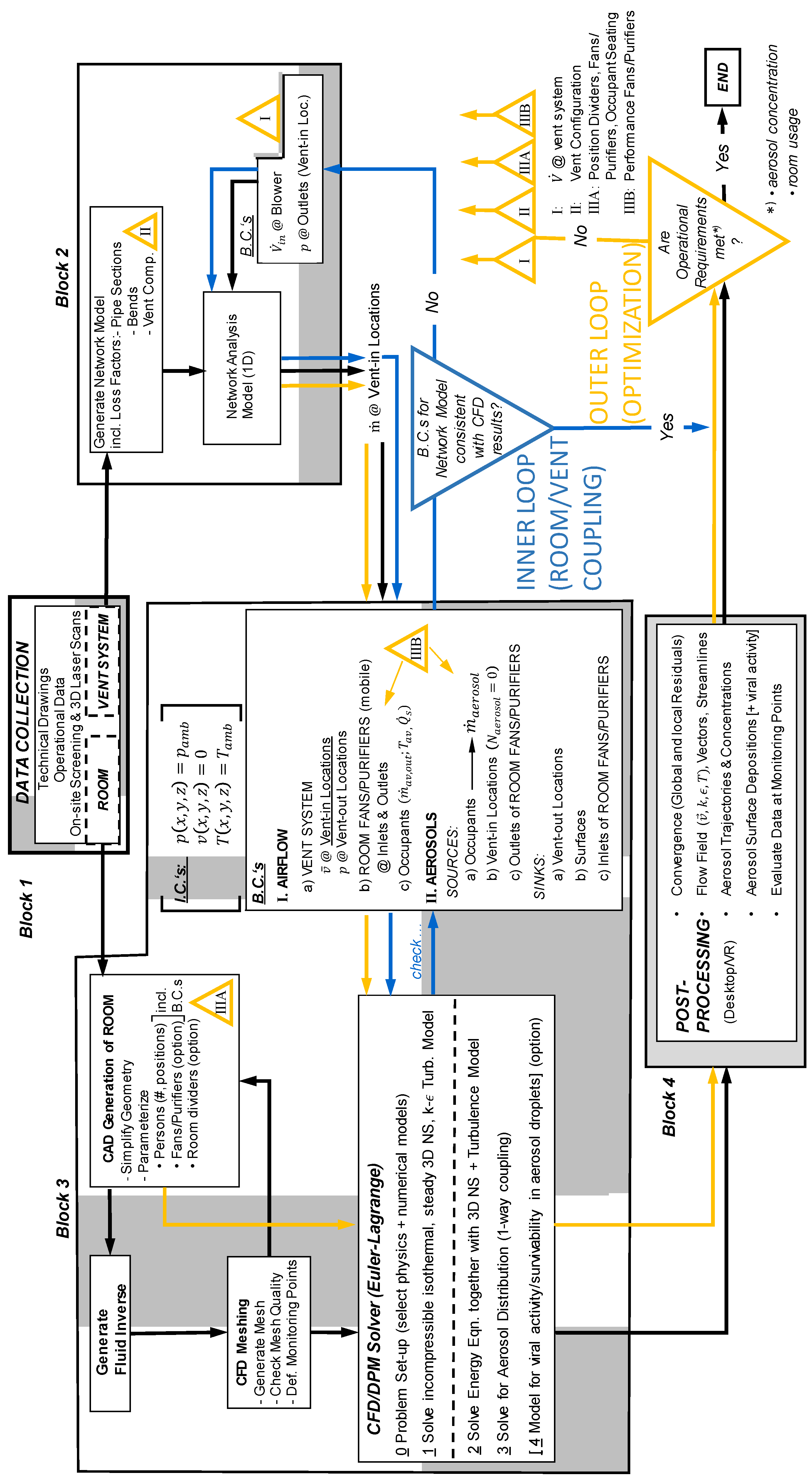
3. Process Workflow
3.1. Overall Flow Field Solution—Room/Vent Coupling (Inner Loop)
- Step 1: calculation of the flow distribution in the venting system based on a reduced-order flow network model;
- Step 2: analysis of the air flow inside the room/lecture hall by means of computational fluid dynamics (CFD) analysis;
- Step 3: extracting the boundary information from Step 2 and repeating Step 1 with the updated information if the old and new boundary information differ by a pre-defined margin.
- Step 4: Solution of the energy equation, alongside mass and momentum conservation equations and based on an initialization using the already calculated isothermal flow field from Step 2. This is necessary in order to account for buoyancy effects due to the higher temperature of the exhaled air and thermal plumes as a consequence of heat transfer from the occupants’ bodies;
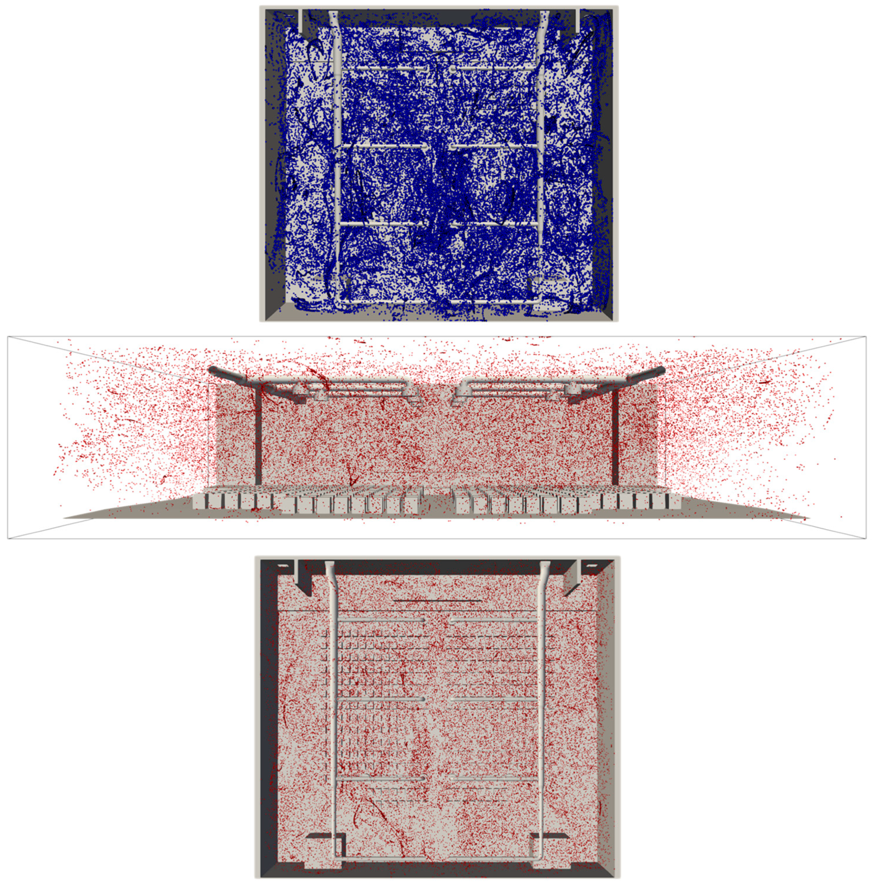
- Step 5: Tracking of aerosol trajectories, allowing for the determination of the aerosol concentration over time within the room (and on surfaces). Here, it is assumed that the aerosol volume concentration in the room is small, such that the room aerodynamics is not influenced by the presence of the aerosol phase; i.e., a one-way coupling between aerosol phase and gas phase is assumed.
3.1.1. Flow Field in the Venting System
3.1.2. Flow Field Within the Lecture Hall
3.2. System Modifications—Optimization (Outer Loop)
Vent System Changes
Changes to Room Interior and/or Occupants
3.3. Workflow Summary
Block 1: Data Collection
Block 2: 1D Network Model/Vent System Flow Distribution
Block 3: CFD Modeling/Room Aerodynamics and Aerosol Distribution
Block 4: Post-Processing Simulation Data
4. Simulation Methods and Models for Test Case
4.1. 1D Network Model—Ventilation System
4.2. 3D CFD Model—Room Aerodynamics and Aerosol Dispersion
Gas-Phase Governing Equations
Disperse-Phase Model
5. Simulation Set-Up
5.1. Material Properties
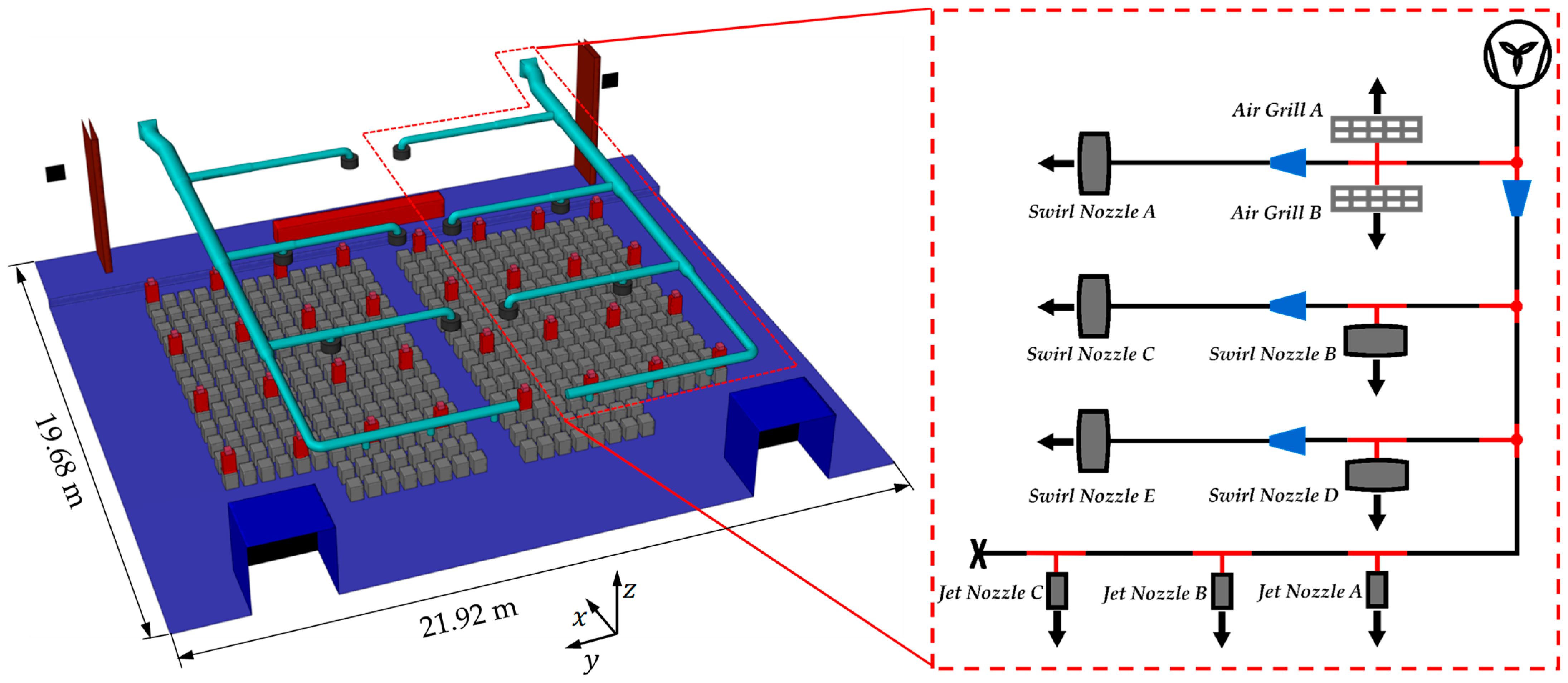
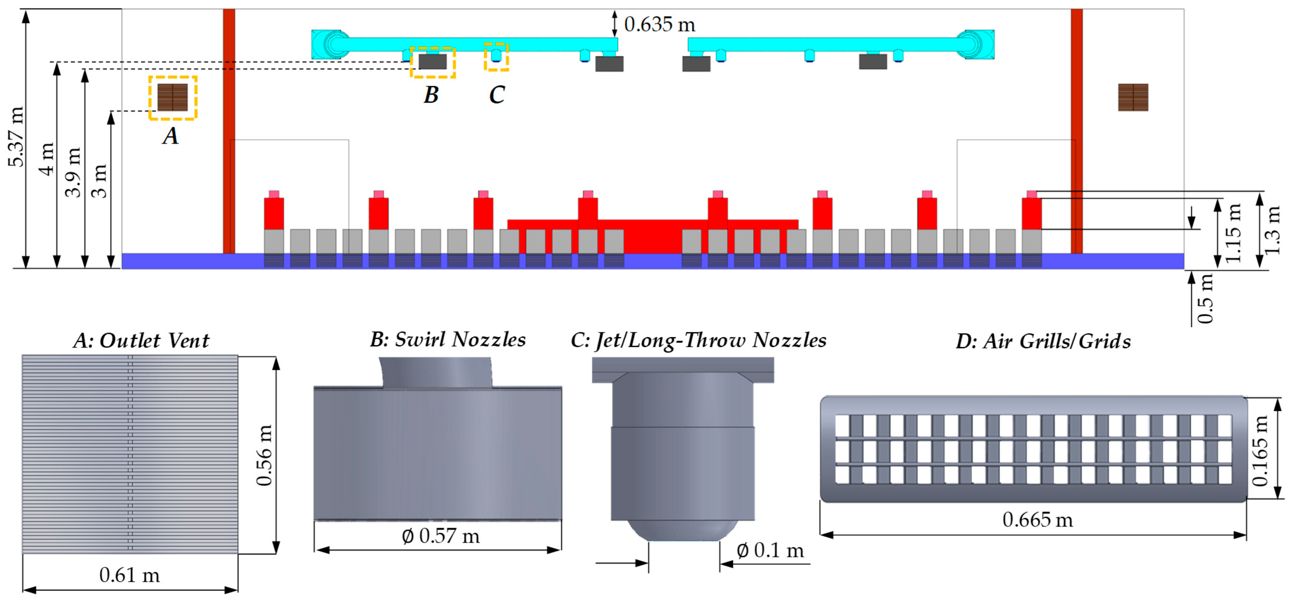
5.2. Vent System Geometry and Boundary Conditions
Room Geometry/CAD Model
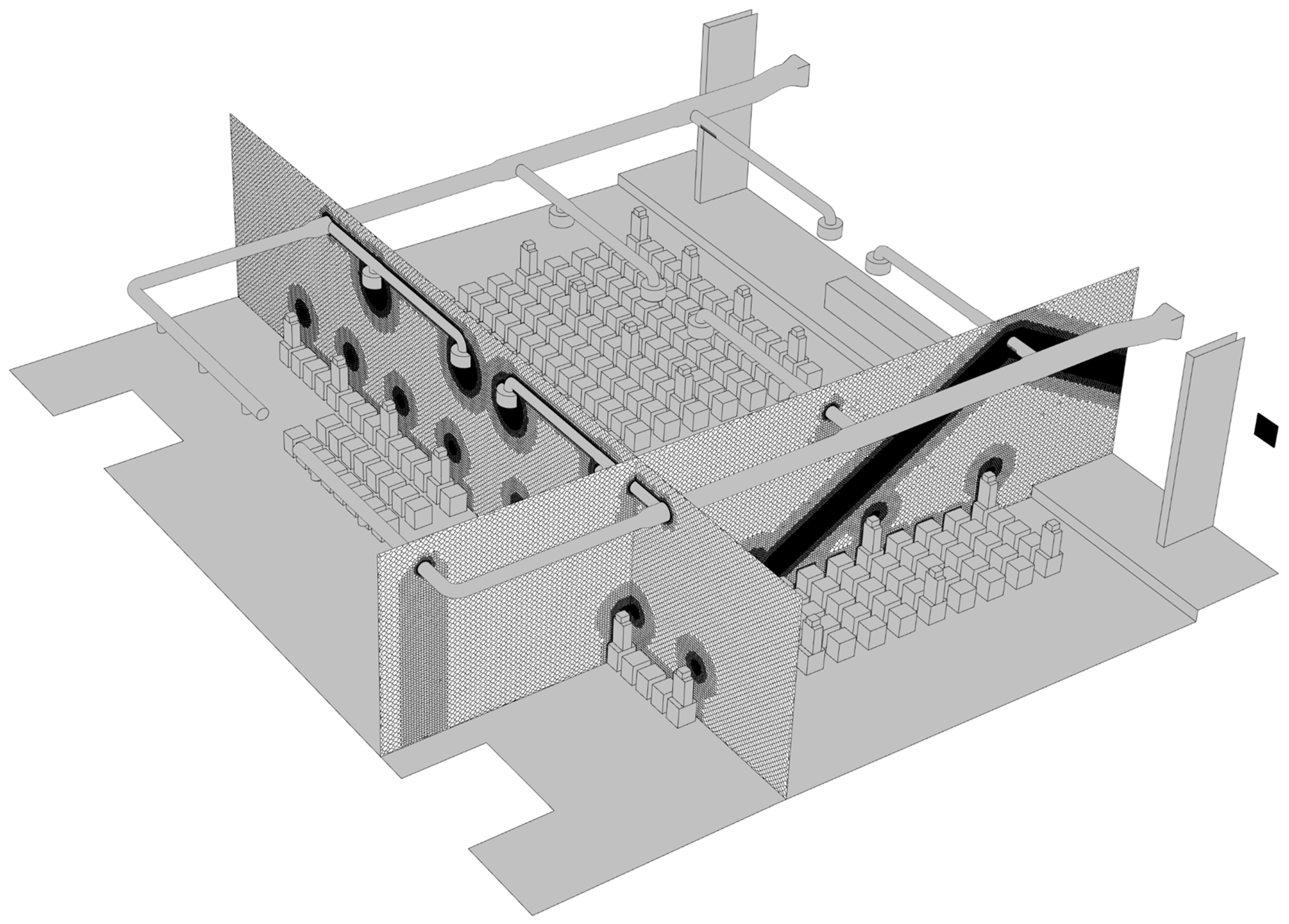
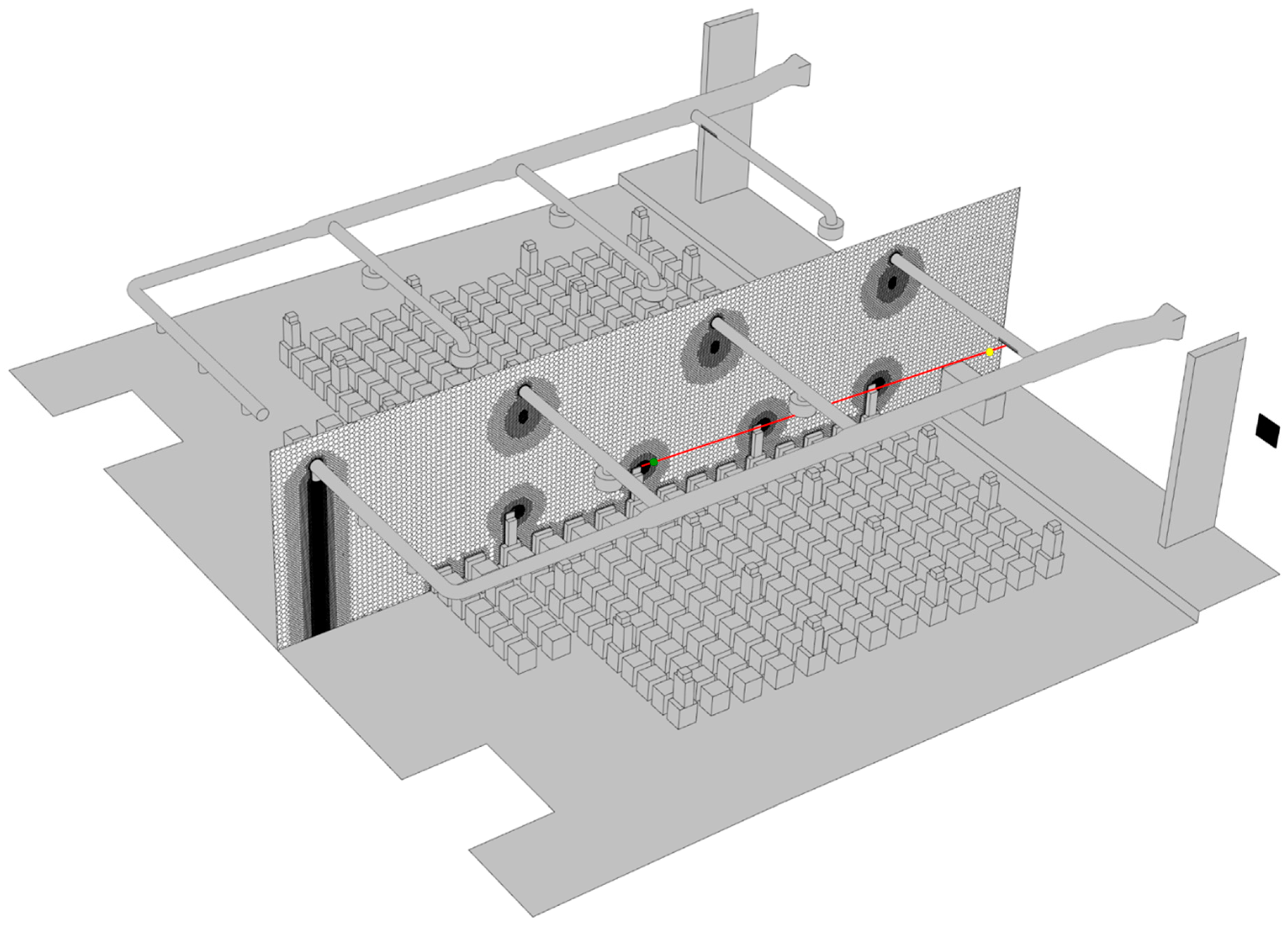
Computational Mesh/Discretization of Flow Domain
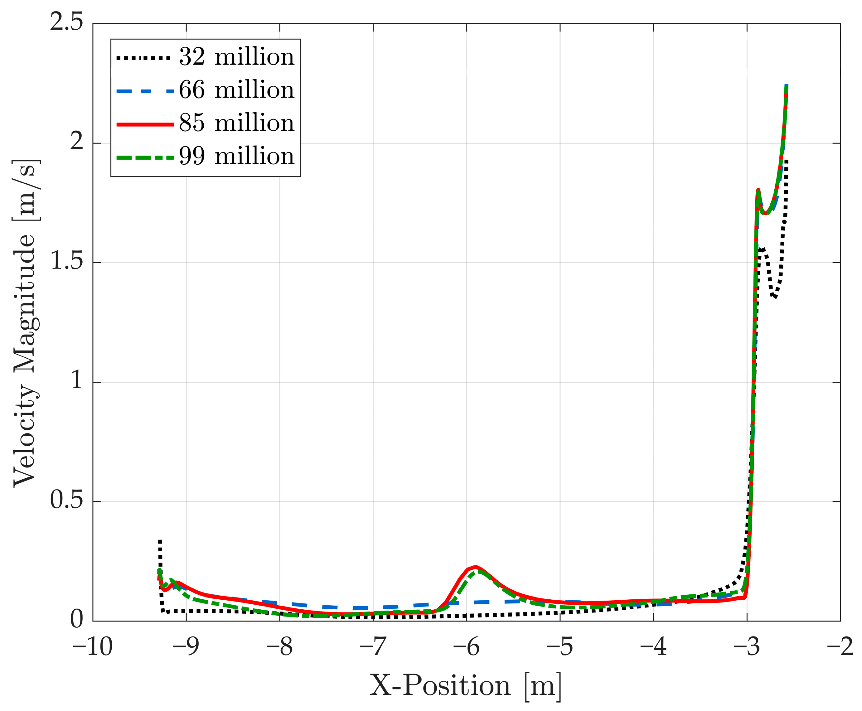
5.3. Mesh Sensitivity Study
5.4. Boundary and Initial Flow-Field Conditions
Boundary Conditions Aerosol Phase/DPM Set-Up
6. Results and Discussion
6.1. Flow Within the Vent System
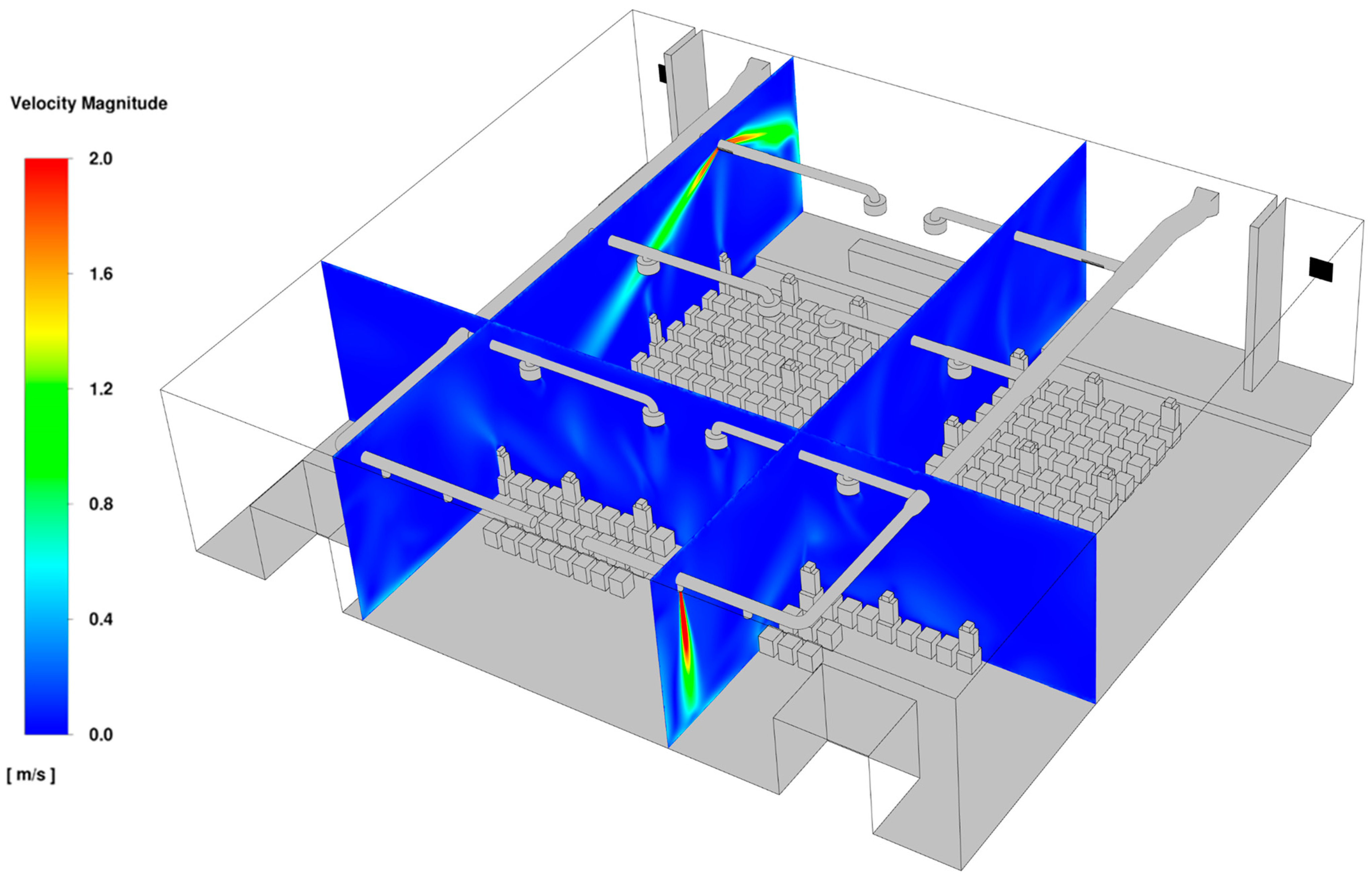
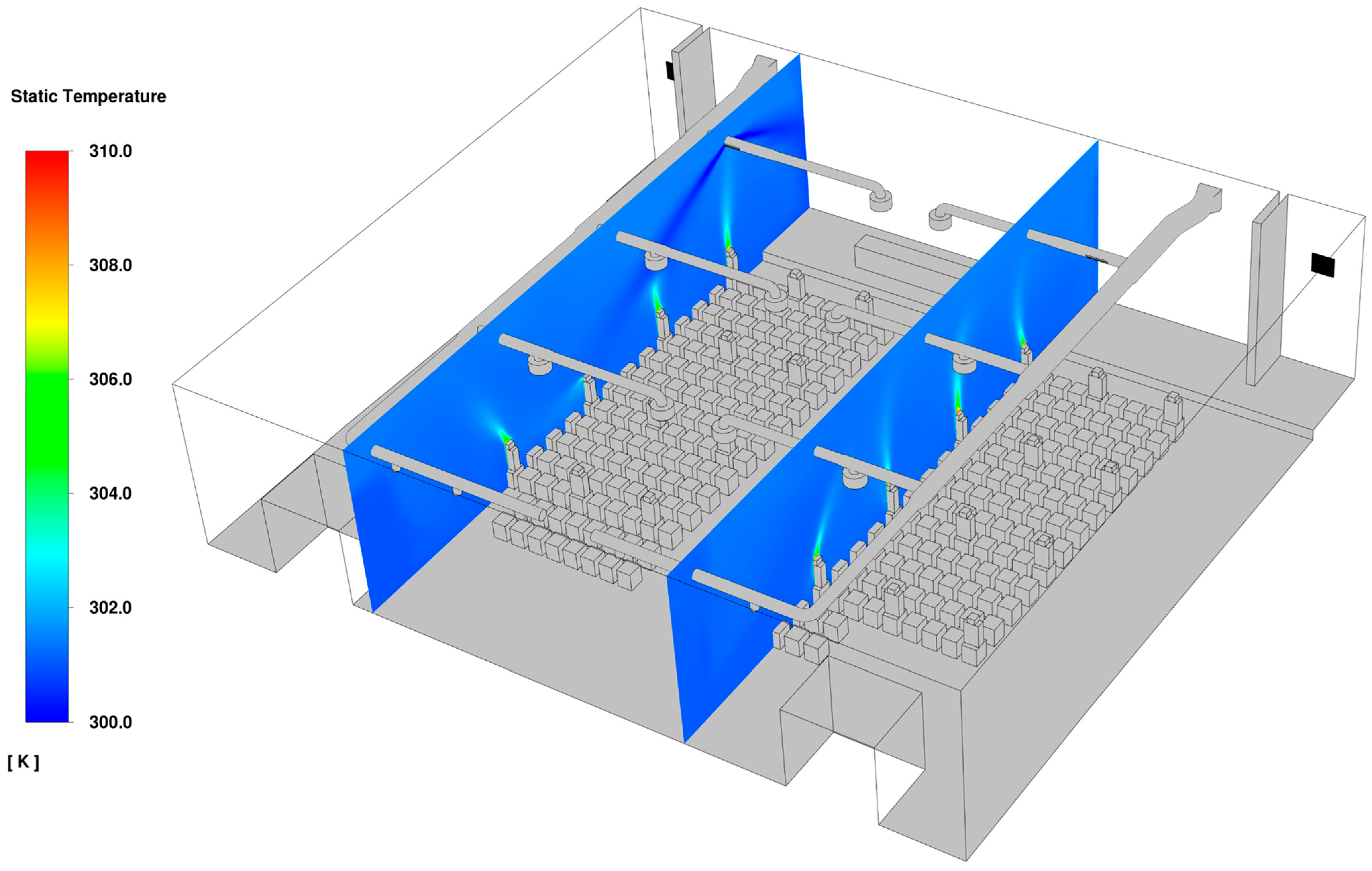
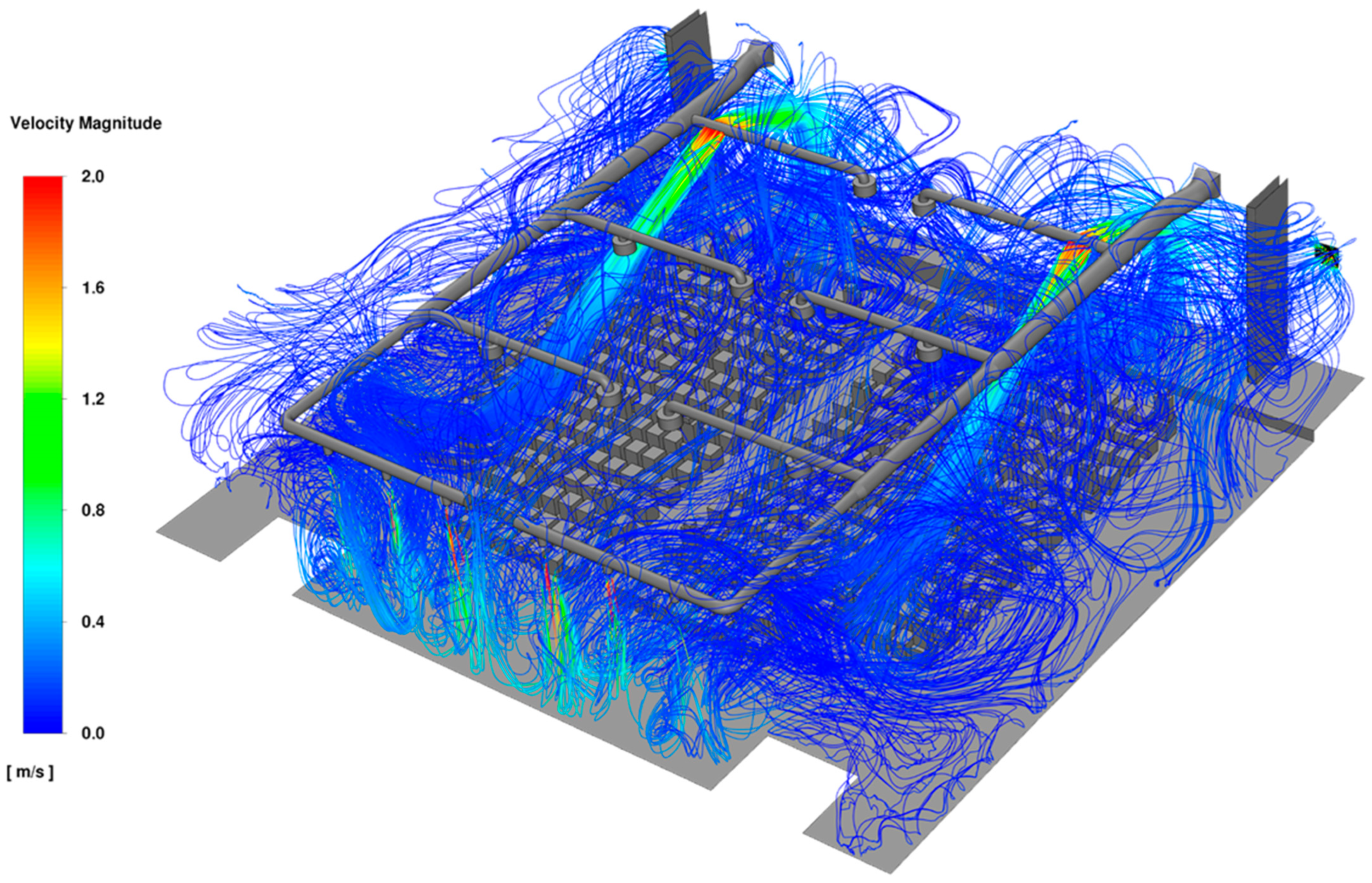
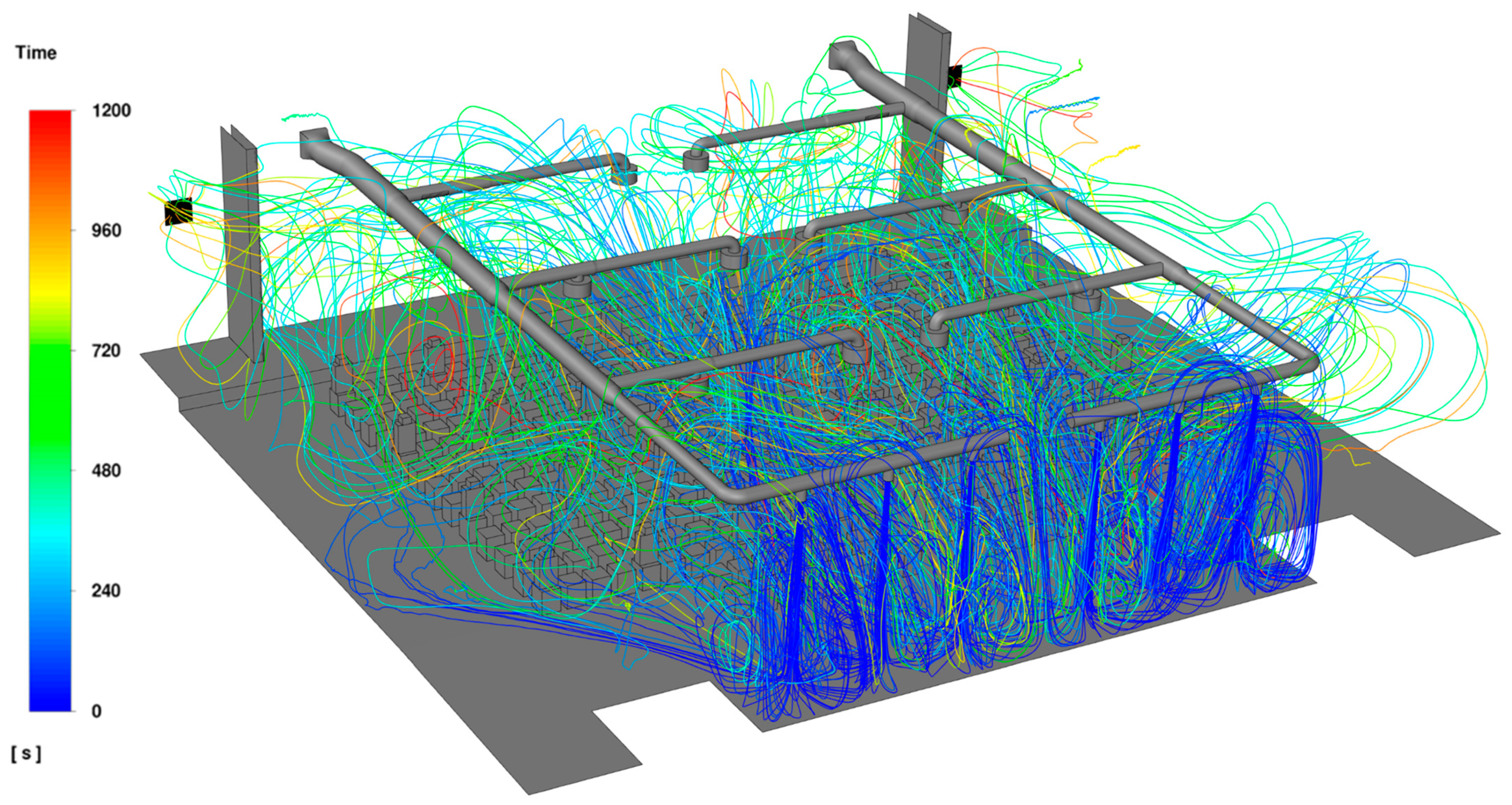
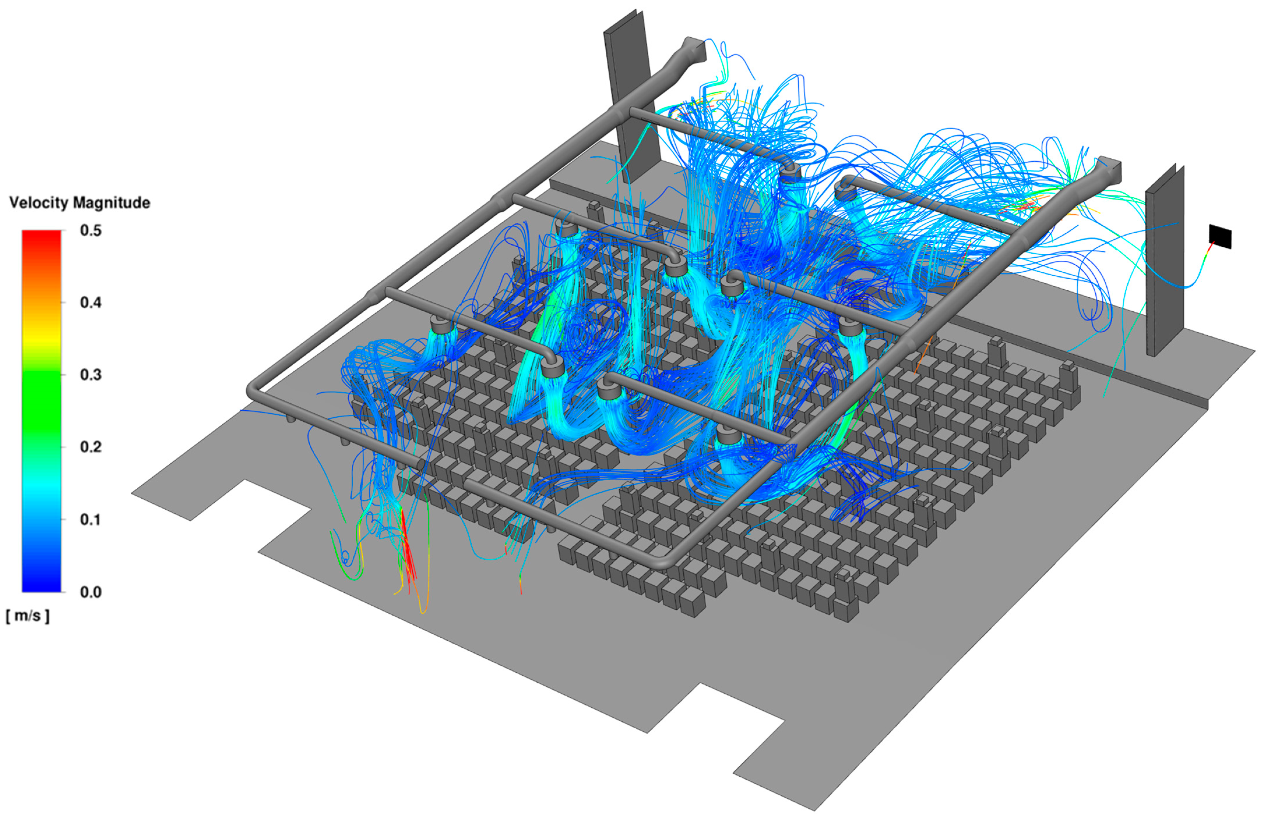
6.2. Flow Field and Aerosol Dispersion Within the Lecture Hall

7. Validation of Model Predictions
8. Conclusions
Author Contributions
Funding
Data Availability Statement
Acknowledgments
Conflicts of Interest
References
- Knibbs, L.D.; Morawska, L.; Bell, S.C.; Grzybowski, P. Room ventilation and the risk of airborne infection transmission in 3 health care settings within a large teaching hospital. Am. J. Infect. Control 2011, 39, 866–872. [Google Scholar] [CrossRef] [PubMed]
- World Health Organization. Roadmap to Improve and Ensure Good Indoor Ventilation in the Context of COVID-19. 2021. Available online: https://www.who.int/publications/i/item/9789240021280 (accessed on 10 March 2025).
- European Centre for Disease Prevention and Control. Heating, Ventilation and Air-Conditioning Systems in the Context of COVID-19: First Update, Stockholm. 2020. Available online: https://www.ecdc.europa.eu/en/publications-data/heating-ventilation-air-conditioning-systems-covid-19 (accessed on 10 March 2025).
- Landesregierung Baden-Württemberg. Verordnung der Landesregierung Über Infektionsschützende Maßnahmen Gegen die Ausbreitung des Virus SARS-CoV-2 (Corona-Verordnung—CoronaVO). Available online: https://www.baden-wuerttemberg.de/fileadmin/redaktion/dateien/PDF/Coronainfos/210423_CoronaVO_konsolidierte_Fassung_ab_210424.pdf (accessed on 10 March 2025).
- BMAS. SARS-CoV-2-Arbeitsschutzregel. 2021. Available online: https://www.bundesanzeiger.de/pub/publication/5QH1uegEXs2GTWXKeln/content/5QH1uegEXs2GTWXKeln/BAnz%20AT%2022.01.2021%20V1.pdf?inline (accessed on 10 March 2025).
- Müller, D.; Rewitz, K.; Derwein, D.; Burgholz, T.M. Vereinfachte Abschätzung des Infektionsrisikos Durch Aerosolgebundene Viren in Belüfteten Räumen; White Paper, RWTH-EBC 2020-005; RWTH Aachen University: Aachen, Germany, 2020. [Google Scholar] [CrossRef]
- Abuhegazy, M.; Talaat, K.; Anderoglu, O.; Poroseva, S.V. Numerical investigation of aerosol transport in a classroom with relevance to COVID-19. Phys. Fluids 2020, 32, 103311. [Google Scholar] [CrossRef] [PubMed]
- Vuorinen, V.; Aarnio, M.; Alava, M.; Alopaeus, V.; Atanasova, N.; Auvinen, M.; Balasubramanian, N.; Bordbar, H.; Erästö, P.; Grande, R.; et al. Modelling aerosol transport and virus exposure with numerical simulations in relation to SARS-CoV-2 transmission by inhalation indoors. Saf. Sci. 2020, 130, 104866. [Google Scholar] [CrossRef]
- Mohamadi, F.; Fazeli, A. A Review on Applications of CFD Modeling in COVID-19 Pandemic. Arch. Comput. Methods Eng. 2022, 29, 3567–3586. [Google Scholar] [CrossRef]
- Arpino, F.; Cortellessa, G.; D’Alicandro, A.C.; Grossi, G.; Massarotti, N.; Mauro, A. CFD analysis of the air supply rate influence on the aerosol dispersion in a university lecture room. Build. Environ. 2023, 235, 110257. [Google Scholar] [CrossRef]
- Mahmoud, M.M.A.; Bahl, P.; Aquino, A.V.d.A.; Maclntyre, C.; Bhattacharjee, S.; Green, D.; Cooper, N.; Doolan, C.; de Silva, C. A numerical framework for the analysis of indoor air quality in a classroom. J. Build. Eng. 2024, 92, 109659. [Google Scholar] [CrossRef]
- Zivelonghi, Y.A.; Lai, M. Mitigating aerosol infection risk in school buildings: The role of natural ventilation, volume, occupancy and CO2 monitoring. Build. Environ. 2021, 204, 108139. [Google Scholar] [CrossRef]
- Aderibigbe, M.; Aliyu, A.M.; Mishra, R. Aerosol Dispersion in Ventilated Rooms: Effect of Built Space Configuration and Facemasks on Indoor Transmission. In Proceedings of the UNIfied Conference of DAMAS, IncoME and TEPEN Conferences (UNIfied 2023), Huddersfield, UK, 29 August–1 September 2023. [Google Scholar]
- Aliyu, A.M.; Singh, D.; Uzoka, C.; Mishra, R. Dispersion of virus-laden droplets in ventilated rooms: Effect of homemade facemasks. J. Build. Eng. 2021, 44, 102933. [Google Scholar] [CrossRef]
- Wei, T.; Xu, H.; Wangda, Z.; Sohn, M.D. Building energy simulation coupled with CFD for indoor environment: A critical review and recent applications. Energy Build. 2018, 165, 184–199. [Google Scholar] [CrossRef]
- Kim, M.; Bordas, R.; Brightling, C.; Chung, Y. A coupled model of 1D-3D CFD to simulate the dynamic flow in airways. Eur. Respir. J. 2016, 48, PA4403. [Google Scholar] [CrossRef]
- Kukutla, P.; Prasad, B. Coupled flow network model and CFD analysis for a combined impingement and film cooled gas turbine nozzle guide vane. Model. Meas. Control B 2017, 86, 250–270. [Google Scholar] [CrossRef]
- Mahmoud, M.M.A.; Aquino, A.F.V.D.A.; Bahl, P.; Maclntyre, C.R.; Green, D.; Doolan, C.; Silva, C.D. Infection Risk Assessment in a Classroom Environment: A CFD Approach with in Situ Aerosol Concentration Measurements. In Proceedings of the 24th Australasian Fluid Mechanics Conference—AFMC2024, Canberra, Australia, 1–5 December 2024. [Google Scholar]
- Tang, H.; Su, Y.; Liu, X.; Li, C.; Yuan, L. Risk assessment of exhaled infectious aerosols transmission driven by natural ventilation in four nursing homes. Build. Simul. 2024, 18, 581–599. [Google Scholar] [CrossRef]
- Rasam, H.; Gentile, V.M.; Tronville, P.; Simonetti, M. Reducing direct exposure to exhaled aerosol through a portable desktop fan. Atmos. Environ. X 2024, 22, 100263. [Google Scholar] [CrossRef]
- Yang, S.; Wang, L.; Raftery, P.; Ivanovich, M.; Taber, C.; Bahnfleth, W.P.; Wargocki, P.; Pantelic, J.; Zou, J.; Mortezazadeh, M.; et al. Comparing airborne infectious aerosol exposures in sparsely occupied large spaces utilizing large-diameter ceiling fans. Build. Environ. 2023, 231, 110022. [Google Scholar] [CrossRef]
- Tao, Y.; Zhong, F.; Miao, Y.; Tang, H.; Li, L. The impact of barrier arrangements on the transmission of respiratory infectious diseases in nursing homes in Hong Kong. Indoor Built Environ. 2024, 33, 1860–1882. [Google Scholar] [CrossRef]
- Technical documentation KG Compact grille, Schako Ferdinand Schad KG, Kolbingen, Germany. 2019. Available online: https://schako.com/wp-content/uploads/kg_en.pdf (accessed on 10 March 2025).
- Technical documentation WDA Long throw nozzle, Schako Ferdinand Schad KG, Kolbingen, Germany. 2021. Available online: https://schako.com/wp-content/uploads/wda_en.pdf (accessed on 10 March 2025).
- Technical Documentation Ceiling Swirl Diffuser DQJ, Schako Ferdinand Schad KG, Kolbingen, Germany. 2020. Available online: https://schako.com/wp-content/uploads/dqj_en.pdf (accessed on 10 March 2025).
- Chourdakis, G.; Davis, K.; Rodenberg, B.; Schulte, M.; Simonis, F.; Uekermann, B.; Abrams, G.; Bungartz, H.-J.; Yau, L.C.; Desai, I.; et al. preCICE v2: A sustainable and user-friendly coupling library. Open Res. Eur. 2022, 2, 51. [Google Scholar] [CrossRef]
- ERCOFTAC Best Practice Guidelines. Industrial Computational Fluid Dynamics of Single-Phase Flows. 2000. Available online: https://www.ercoftac.org/publications/ercoftac_best_practice_guidelines/single-phase_flows_spf/ (accessed on 10 March 2025).
- da Silveira, A.C.; Rodrigues, E.C.; Saleme, E.B.; Covaci, A.; Ghinea, G.; Santos, C.A.S. Thermal and wind devices for multisensory human-computer interaction: An overview. Multimed. Tools Appl. 2023, 82, 34485–34512. [Google Scholar] [CrossRef]
- Guo, Y.; Wang, Y.; Tong, Q.; Shan, B.; He, L.; Zhang, Y.; Wang, D. Active electronic skin: An interface towards ambient haptic feedback on physical surfaces. npj Flex. Electron. 2024, 8, 1–27. [Google Scholar] [CrossRef]
- Flite Software NI Ltd. Piping Systems Fluid Flow 3 Help Manual. 2020. Available online: https://fluidflowinfo.com/ (accessed on 11 March 2025).
- Moody, L.F. Friction Factors for Pipe Flow. Trans. Am. Soc. Mech. Eng. 1944, 66, 671–678. [Google Scholar] [CrossRef]
- Idelchik, I.E. Handbook of Hydraulic Resistance; Begell House Publishers: Danbury, CT, USA, 2001. [Google Scholar]
- Flow of Fluids Through Valves, Fittings, and Pipe; Crane Co.: New York, NY, USA, 1982.
- Lauder, B.; Spalding, D. Lectures in Mathematical Models of Turbulence; Academic Press: London, UK, 1972. [Google Scholar]
- ANSYS Inc. ANSYS Fluent Theory Guide. 2019. Available online: https://www.ansys.com/ (accessed on 11 March 2025).
- Gosman, A.D.; Ioannides, E. Aspects of computer simulation of fluid-fueled combustors. J. Energy 1983, 7, 482–490. [Google Scholar] [CrossRef]
- Oliveira, P.d.; Mesquita, L.; Gkantonas, S.; Giusti, A.; Mastorakos, E. Evolution of spray and aerosol from respiratory releases: Theoretical estimates for insight on viral transmission. Proc. R. Soc. A 2021, 477, 2021. [Google Scholar] [CrossRef] [PubMed]
- Anghel, M.-A.; Iacobescu, F. The Influence of temperature and CO2 in exhaled breath. In Proceedings of the 16th International Congress of Metrology, Paris, France, 7–10 October 2013. [Google Scholar] [CrossRef]
- Balafas, G. Polyhedral Mesh Generation for CFD-Analysis of Complex Structures. München. 2014. Available online: https://api.semanticscholar.org/CorpusID:8490520 (accessed on 10 March 2025).
- Rek, Z.; Rudolf, M.; Zun, I. Application of CFD Simulation in the Development of a New Generation Heating Oven. J. Mech. Eng. 2012, 58, 134–144. [Google Scholar] [CrossRef]
- Wang, W.; Cao, Y.; Okaze, T. Comparison of hexahedral, tetrahedral and polyhedral cells for reproducing the wind field around an isolated building by LES. Build. Environ. 2021, 195, 107717. [Google Scholar] [CrossRef]
- Celik, I.B.; Ghia, U.; Roache, P.J.; Freitas, C.J.; Coleman, H.; Raad, P.E. Procedure for Estimation and Reporting of Uncertainty Due to Discretization in CFD Applications. J. Fluids Eng. 2008, 130, 078001. [Google Scholar] [CrossRef]
- NASA. An Online Resource from NASA on Examining Spatial Grid Convergence. Available online: https://www.grc.nasa.gov/www/wind/valid/tutorial/spatconv.html (accessed on 10 March 2025).
- Roache, P.J. Perspective: A Method for Uniform Reporting of Grid Refinement Studies. ASME J. Fluids Eng. 1994, 116, 405–413. [Google Scholar] [CrossRef]
- Ghorbani, R.; Schmidt, F.M. Fitting of single-exhalation profiles using a pulmonary gas exchange model-application to carbon monoxide. J. Breath Res. 2019, 13, 026001. [Google Scholar] [CrossRef]
- Xu, G.; Antonia, R. Effect of different initial conditions on a turbulent round free jet. Exp. Fluids 2002, 33, 677–683. [Google Scholar] [CrossRef]
- Ball, C.; Fellouah, H.; Pollard, A. The flow field in turbulent round free jets. Prog. Aerosp. Sci. 2012, 50, 1–26. [Google Scholar] [CrossRef]
- DIN EN ISO 7730:2023-04; Ergonomics of the Thermal Environment—Analytical Determination and Interpretation of Thermal Comfort Using Calculation of the PMV and PPD Indices and Local Thermal Comfort; Annex B, Metabolic Rates of Different Activities. ISO: Geneva, Switzerland, 2023.
- Hartmann, A.; Lange, J.; Rotheudt, H.; Kriegel, M. Emissionsrate und Partikelgröße von Bioaerosolen beim Atmen, Sprechen und Husten. 2020. Available online: https://depositonce.tu-berlin.de/items/055a821d-6bd3-462e-9019-33fc6f311362 (accessed on 10 March 2025).
- Pan, S.; Xu, C.; Yu, C.W.F.; Liu, L. Characterization and size distribution of initial droplet concentration discharged from human breathing and speaking. Indoor Built Environ. 2022, 32, 2020–2033. [Google Scholar] [CrossRef]
- Johnson, G.R.; Morawska, L.; Ristovski, Z.D.; Hargreaves, M.; Mengersen, K.; Chao, C.Y.H.; Wan, M.P.; Li, Y.; Xie, X.; Katoshevski, D.; et al. Modality of human expired aerosol size distributions. J. Aerosol Sci. 2011, 42, 839–851. [Google Scholar] [CrossRef]
- Morawska, L.J.G.R.; Johnson, G.R.; Ristovski, Z.D.; Hargreaves, M.; Mengersen, K.; Corbett, S.; Chao, C.Y.H.; Li, Y.; Katoshevski, D. Size distribution and sites of origin of droplets expelled from the human respiratory tract during expiratory activities. J. Aerosol Sci. 2009, 40, 256–269. [Google Scholar] [CrossRef]
- Tu, J.; Wang, M.; Li, W.; Su, J.; Li, Y.; Lv, Z.; Li, H.; Feng, X.; Chen, X. Electronic skins with multimodal sensing and perception. Soft Sci. 2023, 3, 25. [Google Scholar] [CrossRef]
- To, G.N.S.; Wan, M.P.; Chao, C.Y.H.; Fang, L.; Melikov, A. Experimental Study of Dispersion and Deposition of Expiratory Aerosols in Aircraft Cabins and Impact on Infectious Disease Transmission. Aerosol Sci. Technol. 2009, 43, 466–485. [Google Scholar] [CrossRef]
- Memarzadeh, F.; Xu, W. Role of air changes per hour (ACH) in possible transmission of airborne infections. Build. Simul. 2012, 5, 15–28. [Google Scholar] [CrossRef]
- Kek, H.Y.; Saupi, S.B.M.; Tan, H.; Othman, M.H.D.; Nyakuma, B.B.; Goh, P.S.; Altowayti, W.A.H.; Qaid, A.; Wahab, N.H.A.; Lee, C.H.; et al. Ventilation strategies for mitigating airborne infection in healthcare facilities: A review and bibliometric analysis (1993–2022). Energy Build. 2023, 295, 113323. [Google Scholar] [CrossRef]
- Zabihi, M.; Li, R.; Brinkerhoff, J. Influence of indoor airflow on airborne disease transmission in a classroom. Build. Simul. 2024, 17, 355–370. [Google Scholar] [CrossRef]
- Laquerbe, C.; Laborde, J.; Soares, S.; Ricciardi, L.; Floquet, P.; Pibouleau, L.; Domenech, S. Computer aided synthesis of RTD models to simulate the air flow distribution in ventilated rooms. Chem. Eng. Sci. 2001, 56, 5727–5738. [Google Scholar] [CrossRef]

| Equation | |||
|---|---|---|---|
| Continuity | |||
| x-momentum | |||
| y-momentum | |||
| z-momentum | |||
| Energy |
| Equation | |||
|---|---|---|---|
| -equation | |||
| -equation | |||
| , , | |||
| Spatial Discretization | Numerical Scheme |
|---|---|
| Gradient | Least Squares Cell-Based |
| Pressure | Second-Order |
| Momentum | Second-Order Upwind |
| Turbulent Kinetic Energy | Second-Order Upwind |
| Turbulent Dissipation Rate | Second-Order Upwind |
| Energy | Second-Order Upwind |
| No. | Component | K Factor |
|---|---|---|
| 1 | Ventilation Air Grid or Grill | 1.40 |
| 2 | Swirl Nozzle/Diffuser | 20.00 |
| 3 | Jet/Long-Throw Nozzle | 1.14 |
| Grid | Elements [in Millions] | GCI [%] | [-] | |||||||
|---|---|---|---|---|---|---|---|---|---|---|
| #P1 | #P2 | #P1 | #P2 | #P1 | #P2 | #P1 | #P2 | |||
| G1 | 99 | 0.0279 | 0.15 | 1.79 | 1.47 | 0.57 | 10.97 | 9.18 | 1.04 | 1.01 |
| G2 | 66 | 0.0319 | 0.144 | 1.77 | ||||||
| 6.73 | 1.99 | |||||||||
| G3 | 32 | 0.0406 | 0.042 | 1.54 | ||||||
| Boundary Location | Boundary Type | Value |
|---|---|---|
| Occupants’ Mouths | Velocity Inlet | |
| Inlet Vents | Velocity Inlet | see Table 7 |
| Impermeable Surfaces | No-Slip Wall | |
| Outlet Air Grids | Pressure Outlet |
| Serial No. | Component Name | Flowrate [m³/h] | Mean Inlet Velocity [m/s] |
|---|---|---|---|
| 1 | Air Grid A | 568.47 | 2.52 |
| 2 | Air Grid B | 568.47 | 2.52 |
| 3 | Swirl Diffuser/Nozzle A | 126.91 | 0.27 |
| 4 | Swirl Diffuser/Nozzle B | 164.49 | 0.35 |
| 5 | Swirl Diffuser/Nozzle C | 133.93 | 0.28 |
| 6 | Swirl Diffuser/Nozzle D | 121.56 | 0.26 |
| 7 | Swirl Diffuser/Nozzle E | 123.33 | 0.26 |
| 8 | Jet/Long-Throw Nozzle A | 157.21 | 5.56 |
| 9 | Jet/Long-Throw Nozzle B | 173.14 | 6.12 |
| 10 | Jet/Long-Throw Nozzle C | 242.49 | 8.58 |
| Task | Time Consumption [h] |
|---|---|
| Network model | 3.5014 |
| Set-up | 3.5 |
| Calculation | 0.0014 |
| Alternative 1: CAD Generation for Room | 26 |
| In situ measurements in lecture hall | 4 |
| Measurements of flow conditions | 2 |
| HVAC/architecture plan measuring (AutoCAD) | 4 |
| CAD generation in SOLIDWORKS® | 16 |
| Alternative 2: CAD Generation with 3D-Laserscanner Equipment | 13 |
| In situ measurements in lecture hall | 3 |
| Measurements of flow conditions | 2 |
| Post-processing of point cloud data | 8 |
| Mesh Generation | 48 |
| Geometry preparation for pre-processing (DesignModeler) | 2 |
| Meshing set-up (sizing parameters, refinement) | 6 |
| Mesh execution | 10 |
| Check mesh quality and improve mesh (3 iterations) | 30 |
| CFD Simulation + DPM | 16 |
| Conversion of tetrahedral mesh to polyhedral mesh | 2 |
| Definition of boundary conditions | 1 |
| Selection of numerical models and schemes | 1 |
| Run steady simulation without energy equation (5000 iterations); 192 CPU in-house cluster Hydra | 4 |
| Coupling flow with energy equation and run simulation (1000 iterations); 192 CPU in-house cluster Hydra | 1 |
| DPM set-up | 1 |
| Calculation of particle trajectories | 6 |
| Post-Processing | 12 |
| CFD and DPM results | 10 |
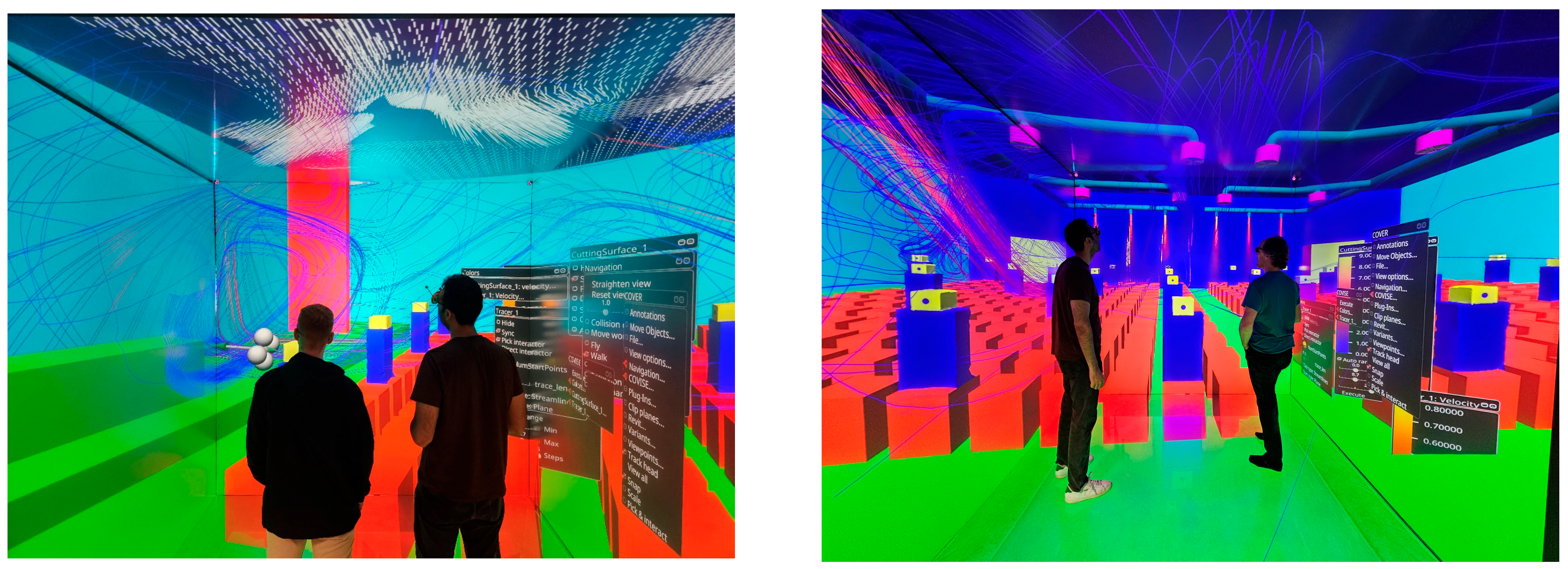
| Visualization of results (VR via CAVE) | 2 |
| Total Time Consumption | 118.5014 |
| S. No. | Location | Simulation [m/s] | Experiment | Percentage Error |
|---|---|---|---|---|
| 1 | Jet/Long-Throw Exit Nozzle C | 8.58 (1D network) | 8.06–8.3 m/s (±0.03 m/s + 5% of measured value) | 4.89% |
| 2 | Jet/Long-Throw Nozzle B (measured 1.5 m below the nozzle outlet) | 2.72 (3D CFD) | 2.74–2.99 m/s (±0.03 m/s + 5% of measured value) | 5.06% |
| 3 | Outlet 1 (right side of the lecture hall) | 3.754 (3D CFD) | 3.6–4.2 m/s (±0.03 m/s + 5% of measured value) | 3.74% |
Disclaimer/Publisher’s Note: The statements, opinions and data contained in all publications are solely those of the individual author(s) and contributor(s) and not of MDPI and/or the editor(s). MDPI and/or the editor(s) disclaim responsibility for any injury to people or property resulting from any ideas, methods, instructions or products referred to in the content. |
© 2025 by the authors. Licensee MDPI, Basel, Switzerland. This article is an open access article distributed under the terms and conditions of the Creative Commons Attribution (CC BY) license (https://creativecommons.org/licenses/by/4.0/).
Share and Cite
Ajmani, A.; Kirchhof, L.; Rouhi, A.; Mehring, C. Assessing the Effect of Air Ventilation on the Dispersion of Exhaled Aerosol Particles in a Lecture Hall: Simulation Strategy and Streamlined Workflow. Fluids 2025, 10, 132. https://doi.org/10.3390/fluids10050132
Ajmani A, Kirchhof L, Rouhi A, Mehring C. Assessing the Effect of Air Ventilation on the Dispersion of Exhaled Aerosol Particles in a Lecture Hall: Simulation Strategy and Streamlined Workflow. Fluids. 2025; 10(5):132. https://doi.org/10.3390/fluids10050132
Chicago/Turabian StyleAjmani, Arnav, Lars Kirchhof, Alireza Rouhi, and Carsten Mehring. 2025. "Assessing the Effect of Air Ventilation on the Dispersion of Exhaled Aerosol Particles in a Lecture Hall: Simulation Strategy and Streamlined Workflow" Fluids 10, no. 5: 132. https://doi.org/10.3390/fluids10050132
APA StyleAjmani, A., Kirchhof, L., Rouhi, A., & Mehring, C. (2025). Assessing the Effect of Air Ventilation on the Dispersion of Exhaled Aerosol Particles in a Lecture Hall: Simulation Strategy and Streamlined Workflow. Fluids, 10(5), 132. https://doi.org/10.3390/fluids10050132