Modified Semi-Lagrangian Godunov-Type Method Without Numerical Viscosity for Shocks

Abstract

Most high-order Euler-type methods have been proposed to solve one-dimensional scalar hyperbolic conservational law. These methods resolve smooth variations in flow parameters accurately and simultaneously identify the discontinuities. A disadvantage of Euler-type methods is the parameter change stretching in the shock over a few mesh cells. In reality, in the shock, the flow properties change abruptly at once for the computational mesh. In our considerations, the mean free path of a flow particle is much smaller than the mesh cell size. This paper describes a modification of the semi-Lagrangian Godunov-type method, which was proposed by the author in the previously published paper. The modified method also does not have numerical viscosity for shocks. In the previous article, a linear law for the distribution of flow parameters was employed for a rarefaction wave when modeling the Shu-Osher problem with the aim of reducing parasitic oscillations. Additionally, the nonlinear law derived from the Riemann invariants was used for the remaining test problems. This article proposes an advanced method, namely, a unified formula for the density distribution of rarefaction waves and modification of the scheme for modeling moderately strong shock waves. The obtained results of numerical analysis, including the standard problem of Sod, the Riemann problem of Lax, the Shu–Osher shock-tube problem and a few author’s test cases are compared with the exact solution, the data of the previous method and the Total Variation Deminishing (TVD) scheme results. This article delineates the further advancement of the numerical scheme of the proposed method, specifically presenting a unified mathematical formulation for an expanded set of test problems.

1. Introduction

Compressible flows simulation presents a significant challenge due to the existence of discontinuities in the fluid flow, including shocks, contact waves, and a wide range of continuous flow scales. To address these challenges, various high-resolution methods have been developed to accurately resolve smooth flow scales while simultaneously capturing discontinuities. All numerical methods can be categorized into direct numerical simulation (DNS) [1,2,3,4,5,6,7,8,9,10,11,12,13,14,15,16,17], large eddy simulation (LES) [18,19], and Reynolds-averaged Navier–Stokes simulation (RANS) [20,21,22]. The method proposed in this paper belongs to the class of DNS methods.

Notable examples include the artificial viscosity method [1,2], the total variation diminishing (TVD) method [3], the essentially non-oscillatory (ENO) scheme [4], and the weighted essentially non-oscillatory (WENO) scheme [5]. Harten et al. developed the ENO scheme [4,6,7,8], the first successful high-order method to allow the spatial discretization of hyperbolic conservation laws. This property is very useful for the numerical simulation of hyperbolic conservation laws because high-order numerical methods often cause false vibrations, especially near shocks or other interruptions. The spatial discretization of finite volumes of ENO has been studied [4], where it has been shown that it is uniformly accurate in the capturing of the location of any discontinuity in the flow. Subsequently, Shu and Osher [9,10] developed a finite difference ENO scheme. The main idea of the ENO scheme is to select the interpolation point stencil that suppresses the oscillations, i.e., to choose the best solution varying stencil, to approximate the cell boundary flow, and to avoid large false oscillations caused by interpolating data between discontinuities.

WENO schemes have been studied [5,11,12] to deal with potential numerical instability when selecting ENO stencils. The WENO method applies to a convex combination of all ENO stencils, which obtains higher precision in smooth regions than the ENO method while maintaining the ENO property at discontinuities.

The abovementioned methods belong to the class of Euler-type methods. These methods [1,2,3,4,5,6,7,8,9,10,11,12,13] exhibit numerical viscosity in the presence of shocks. Additionally, methods exist [14,15,16,17] that incorporate exact Riemann solutions while still being classified as Euler-type methods, which also exhibit numerical viscosity for shocks. Godunov et al. [14] proposed mitigating this issue by using moving grids; however, this approach significantly complicates the problem, particularly in multi-dimensional cases.

For highly rarefied gases, in particular, the direct simulation Monte Carlo (DSMC) method is applied, in the numerical scheme of which the fact of instantaneous change in flow parameters on shock waves is used [23].

In [24], we proposed a Lagrangian Godunov-type method that eliminates the numerical viscosity for shocks and provided a detailed description of the wall conditions. The method utilizes a fixed homogeneous grid. This paper presents a modified method that involves altering the formula for the density calculation in rarefaction waves. It was found that this formula allows obtaining good results for all types of test problems solved in [24]. While in work [24], two different formulas were used to obtain successful results: the linear law of the distribution of flow parameters in a rarefaction wave for the Shu and Osher shock tube problem [25] and the nonlinear law for the remaining problems of consideration. In addition, the following innovation is proposed here, which consists of considering an additional condition on the direction of the shock wave at the stage of calculating the acoustic substep. Moreover, this innovation, introduced into the scheme of the method, does not affect the results of the test problems already considered in [24], but manifests itself only in the numerical solution of the two last test cases of the interaction of two Riemann problems presented in this work.

2. Materials and Methods

In the case of the one-dimensional scalar hyperbolic conservation law [13], the equations are given as follows:

$$\begin{array}{l}{\displaystyle \frac{𝜕\rho }{𝜕\mathrm{t}}}+\mathrm{u}{\displaystyle \frac{𝜕\rho }{𝜕\mathrm{x}}}+\rho {\displaystyle \frac{𝜕\mathrm{u}}{𝜕\mathrm{x}}}=0,\\ {\displaystyle \frac{𝜕\mathrm{u}}{𝜕\mathrm{t}}}+\mathrm{u}{\displaystyle \frac{𝜕\mathrm{u}}{𝜕\mathrm{x}}}+{\displaystyle \frac{1}{\rho }}{\displaystyle \frac{𝜕\mathrm{p}}{𝜕\mathrm{x}}}=0,\\ {\displaystyle \frac{𝜕\epsilon }{𝜕\mathrm{t}}}+\mathrm{u}{\displaystyle \frac{𝜕\epsilon }{𝜕\mathrm{x}}}+{\displaystyle \frac{\mathrm{p}}{\rho }}{\displaystyle \frac{𝜕\mathrm{u}}{𝜕\mathrm{x}}}=0.\end{array}$$

(1)

Here, u is the convective velocity of flow, $\rho$ is the density, $\mathrm{p}$ is the pressure, $\epsilon$ is the internal specific energy, x is the direction, and t is the time.

The pressure is determined using the equation of state

$$\mathrm{p}=(\kappa -1) \rho \epsilon .$$

(2)

where $\kappa$ is the ratio of specific heat coefficients at constant pressure and volume. For air, $\kappa =1.4$.

Godunov et al. [14] proposed an iterative exact Riemann solver, which was implemented in a finite-difference scheme. Later, other researchers adopted a control volume method instead, while we employed the Lagrangian approach.

In this paper, as well as in a previous paper [24], the following method is proposed: The convection and acoustic stages are considered separately and are classified as distinct physical processes because the local acoustic velocity (i.e., sound speed) can vary significantly from the flow convection velocity. Therefore, we solve the following system during the acoustic stage:

$$\begin{array}{l}{\displaystyle \frac{𝜕\rho }{𝜕\mathrm{t}}}+\rho {\displaystyle \frac{𝜕\mathrm{u}}{𝜕\mathrm{x}}}=0,\\ {\displaystyle \frac{𝜕\mathrm{u}}{𝜕\mathrm{t}}}+{\displaystyle \frac{1}{\rho }}{\displaystyle \frac{𝜕\mathrm{p}}{𝜕\mathrm{x}}}=0,\\ {\displaystyle \frac{𝜕\epsilon }{𝜕\mathrm{t}}}+{\displaystyle \frac{\mathrm{p}}{\rho }}{\displaystyle \frac{𝜕\mathrm{u}}{𝜕\mathrm{x}}}=0.\end{array}$$

(3)

and Equation (2). The system (3) is derived from (1) by discarding the convective terms and can be expressed in a matrix form as follows:

$$\left\{\begin{array}{c}{\displaystyle \frac{𝜕\rho }{𝜕\mathrm{t}}}\\ {\displaystyle \frac{𝜕\mathrm{u}}{𝜕\mathrm{t}}}\\ {\displaystyle \frac{𝜕\epsilon }{𝜕\mathrm{t}}}\end{array}\right\}=\left[\mathrm{A}\right]\left\{\begin{array}{c}{\displaystyle \frac{𝜕\rho }{𝜕\mathrm{x}}}\\ {\displaystyle \frac{𝜕\mathrm{u}}{𝜕\mathrm{x}}}\\ {\displaystyle \frac{𝜕\epsilon }{𝜕\mathrm{x}}}\end{array}\right\}$$

(4)

where $\left[\mathrm{A}\right]$ is the Jacobian matrix:

$$\left[\mathrm{A}\right]=\left[\begin{array}{ccc}0& \rho & 0\\ {\displaystyle \frac{(\kappa -1)\epsilon }{\rho }}& 0& \kappa -1\\ 0& (\kappa -1)\epsilon & 0\end{array}\right].$$

(5)

The matrix $\left[\mathrm{A}\right]$ can be expressed as

$$\left[\mathrm{A}\right]=\left[\mathrm{R}\right]\left[\Lambda \right]\left[\mathrm{L}\right],$$

(6)

where $[\Lambda ]$ is the diagonal matrix of eigenvalues of the matrix $\left[\mathrm{A}\right]$.

$$\left[\Lambda \right]=\left[\begin{array}{ccc}-\mathrm{c}& 0& 0\\ 0& 0& 0\\ 0& 0& \mathrm{c}\end{array}\right].$$

(7)

Here $\mathrm{c}$ is the sound velocity, which is determined as follows:

$$\mathrm{c}=\sqrt{\kappa {\displaystyle \frac{\mathrm{p}}{\rho }}},$$

(8)

A corresponding left-eigenvector matrix $[\mathrm{L}]$, determined as

$$\left[\mathrm{L}\right]=\left[\begin{array}{ccc}-{\displaystyle \frac{\mathrm{c}}{\kappa \rho }}& 1& -{\displaystyle \frac{\kappa -1}{\mathrm{c}}}\\ 1& 0& -{\displaystyle \frac{\rho \kappa }{{\mathrm{c}}^2}}\\ {\displaystyle \frac{\mathrm{c}}{\kappa \rho }}& 1& {\displaystyle \frac{\kappa -1}{\mathrm{c}}}\end{array}\right]$$

(9)

and a corresponding right eigenvectors matrix $[\mathrm{R}]$, defined as

$$\left[\mathrm{R}\right]=\left[\begin{array}{ccc}-{\displaystyle \frac{\rho }{2\mathrm{c}}}& {\displaystyle \frac{\kappa -1}{\kappa }}& {\displaystyle \frac{\rho }{2\mathrm{c}}}\\ {\displaystyle \frac{1}{2}}& 0& {\displaystyle \frac{1}{2}}\\ -{\displaystyle \frac{\mathrm{c}}{2\kappa }}& -{\displaystyle \frac{(\kappa -1)\epsilon }{\kappa \rho }}& {\displaystyle \frac{\mathrm{c}}{2\kappa }}\end{array}\right].$$

(10)

Since

$$\left[\mathrm{L}\right]\left[\mathrm{R}\right]=\left[\mathrm{E}\right],$$

(11)

where $\left[\mathrm{E}\right]$ is a diagonal identity matrix, multiplying Equation (4) from the left by $\left[\mathrm{L}\right]$ and applying (11) results in the following:

$$\left[\mathrm{L}\right]\left\{\begin{array}{c}{\displaystyle \frac{𝜕\rho }{𝜕\mathrm{t}}}\\ {\displaystyle \frac{𝜕\mathrm{u}}{𝜕\mathrm{t}}}\\ {\displaystyle \frac{𝜕\epsilon }{𝜕\mathrm{t}}}\end{array}\right\}=\left[\Lambda \right]\left[\mathrm{L}\right]\left\{\begin{array}{c}{\displaystyle \frac{𝜕\rho }{𝜕\mathrm{x}}}\\ {\displaystyle \frac{𝜕\mathrm{u}}{𝜕\mathrm{x}}}\\ {\displaystyle \frac{𝜕\epsilon }{𝜕\mathrm{x}}}\end{array}\right\}.$$

(12)

If $\left[\mathrm{L}\right]=[\mathrm{c}\mathrm{o}\mathrm{n}\mathrm{s}\mathrm{t}]$, from (12) we can obtain the characteristic form:

$$\begin{array}{c}{\displaystyle \frac{𝜕{\mathrm{w}}_1}{𝜕\mathrm{t}}}-\mathrm{c}{\displaystyle \frac{𝜕{\mathrm{w}}_1}{𝜕\mathrm{x}}}=0,\\ {\displaystyle \frac{𝜕{\mathrm{w}}_2}{𝜕\mathrm{t}}}=0, \\ {\displaystyle \frac{𝜕{\mathrm{w}}_3}{𝜕\mathrm{t}}}+\mathrm{c}{\displaystyle \frac{𝜕{\mathrm{w}}_3}{𝜕\mathrm{x}}}=0,\end{array}$$

(13)

where

$$\begin{array}{c}{\mathrm{w}}_1=-{\displaystyle \frac{\mathrm{c}*}{\kappa \rho *}}\rho +\mathrm{u}-{\displaystyle \frac{\kappa -1}{\mathrm{c}*}}\epsilon ,\\ {\mathrm{w}}_2=\rho -{\displaystyle \frac{\kappa \rho *}{{\mathrm{c}*}^2}}\epsilon , \\ {\mathrm{w}}_3={\displaystyle \frac{\mathrm{c}*}{\kappa \rho *}}\rho +\mathrm{u}+{\displaystyle \frac{\kappa -1}{\mathrm{c}*}}\epsilon .\end{array}$$

(14)

Here, an asterisk represents constant values. Equation (13) describes the motion of two waves with velocities $-\mathrm{c}$ and $\mathrm{c}$. The waves transfer the values ${\mathrm{w}}_1$ and ${\mathrm{w}}_3$ as given in (14), respectively.

The proposed Lagrangian approach can be used to solve the system of Equation (13). However, as in the previous paper [24], we use the Godunov exact solver to solve the full nonlinear systems (1) and (2). We then subtract the convective velocity from the solution to obtain the solution of Equation (3). For more details, see below.

We accept the time step ${}_{\Delta }\mathrm{t}_{\mathrm{c}}$ at the acoustic stage in accordance with the Courant criterion:

$${}_{\Delta }\mathrm{t}_{\mathrm{c}}={\mathrm{k}}_{\mathrm{c}}{\displaystyle \frac{\mathrm{h}}{{\mathrm{c}}_{\mathrm{s}}}},$$

(15)

where ${\mathrm{c}}_{\mathrm{s}}$ is the shock acoustic velocity and ${\mathrm{k}}_{\mathrm{c}}$ is integer. For example, if ${\mathrm{k}}_{\mathrm{c}}=3$, then the shock spreads through three grid cells during the acoustic stage.

During the convection stage, only the system with convective terms is solved:

$$\begin{array}{c}{\displaystyle \frac{𝜕\rho }{𝜕\mathrm{t}}}+\mathrm{u}{\displaystyle \frac{𝜕\rho }{𝜕\mathrm{x}}}=0,\\ {\displaystyle \frac{𝜕\mathrm{u}}{𝜕\mathrm{t}}}+\mathrm{u}{\displaystyle \frac{𝜕\mathrm{u}}{𝜕\mathrm{x}}}=0,\\ {\displaystyle \frac{𝜕\epsilon }{𝜕\mathrm{t}}}+\mathrm{u}{\displaystyle \frac{𝜕\epsilon }{𝜕\mathrm{x}}}=0.\end{array}$$

(16)

as well as Equation (13).

The time step during the convection stage is taken to be similar to that of (15):

$${}_{\Delta }\mathrm{t}_{\mathrm{u}}={\mathrm{k}}_{\mathrm{u}}{\displaystyle \frac{\mathrm{h}}{{\mathrm{u}}_{\mathrm{s}}}},$$

(17)

where ${\mathrm{u}}_{\mathrm{s}}$ is the shock convective velocity and ${\mathrm{k}}_{\mathrm{u}}$ is integer. For example, if ${\mathrm{k}}_{\mathrm{u}}=2$, then the shock spreads through two grid cells at the convection stage. If ${}_{\Delta }\mathrm{t}_{\mathrm{c}}\ne {}_{\Delta }\mathrm{t}_{\mathrm{u}}$, then the marching time steps ${}_{\Delta }\mathrm{t}$ is chosen so that

$$\begin{array}{c}{}_{\Delta }\mathrm{t}_{\mathrm{c}}={\mathrm{n}}_{\mathrm{c}}{}_{\Delta }\mathrm{t},\\ {}_{\Delta }\mathrm{t}_{\mathrm{u}}={\mathrm{n}}_{\mathrm{u}}{}_{\Delta }\mathrm{t},\end{array}$$

(18)

where ${\mathrm{n}}_{\mathrm{c}}$ and ${\mathrm{n}}_{\mathrm{u}}$ are integers.

2.1. A Methodological Scheme During the Acoustics Stage

During the acoustics stage, the system of Equation (3) is solved. Although the wave equation system (13) cannot be derived for a nonlinear problem, the fundamental properties of the linear system (13) are retained in the nonlinear system (3). The topologies of the nonlinear and linear systems are identical. This phenomenon corresponds to either a shock wave or a rarefaction wave [14]. Unfortunately, the variables ${\mathrm{w}}_1$ and ${\mathrm{w}}_3$ for the nonlinear system (3) are unknown. However, the exact solution of the Riemann problem for the nonlinear systems (1) and (2) can be determined using the Godunov method [14]. This solution is represented using the large variables: ${\mathrm{R}}_{\mathrm{L}}$ and ${\mathrm{R}}_{\mathrm{R}}$ for density, ${\mathrm{U}}_{\mathrm{L}}={\mathrm{U}}_{\mathrm{R}}$ for speed, ${\mathrm{E}}_{\mathrm{L}}$ and ${\mathrm{E}}_{\mathrm{R}}$ for internal specific energy, ${\mathrm{P}}_{\mathrm{L}}={\mathrm{P}}_{\mathrm{R}}$ for pressure, ${\mathrm{D}}_{\mathrm{L}}$ and ${\mathrm{D}}_{\mathrm{R}}$ for the propagation velocity frequency of shock or rarefaction waves. The subscripts $\mathrm{L}$ and $\mathrm{R}$ denote the left and right cells adjacent to the edge between them.

In the proposed method, ${\mathrm{w}}_1$ and ${\mathrm{w}}_3$ (14) are replaced by ${\overline{\mathrm{w}}}_1{ =\{\mathrm{P}}_{\mathrm{L}}{, \mathrm{U}}_{\mathrm{L}}, {\mathrm{R}}_{\mathrm{L}}{, \mathrm{E}}_{\mathrm{L}}\}$ and ${\overline{\mathrm{w}}}_3{ =\{\mathrm{P}}_{\mathrm{R}}{, \mathrm{U}}_{\mathrm{R}}, {\mathrm{R}}_{\mathrm{R}}{, \mathrm{E}}_{\mathrm{R}}\}$, which are each transported by the local acoustic velocities ${\mathrm{C}}_{\mathrm{L}}={\mathrm{D}}_{\mathrm{L}}-{\mathrm{U}}_{\mathrm{L}}$ and ${\mathrm{C}}_{\mathrm{R}}={\mathrm{D}}_{\mathrm{R}}-{\mathrm{U}}_{\mathrm{R}}$.

First, we must solve the Riemann problem using the Godunov method [14] for each pair of cells ($\mathrm{i}$ and $\mathrm{i}+1$) with the corresponding data ($\left\{{\mathrm{p}}_{\mathrm{i}},{\mathrm{u}}_{\mathrm{i}},{\rho }_{\mathrm{i}},{\epsilon }_{\mathrm{i}}\right\}$ and $\left\{{\mathrm{p}}_{\mathrm{i}+1},{\mathrm{u}}_{\mathrm{i}+1},{\rho }_{\mathrm{i}+1},{\epsilon }_{\mathrm{i}+1}\right\}$), respectively. Therefore, the values of the large variables $\{\mathrm{P}, \mathrm{U}, {\mathrm{R}}_{\mathrm{L}}, {\mathrm{E}}_{\mathrm{L}}, {\mathrm{D}}_{\mathrm{L}}, {\mathrm{R}}_{\mathrm{R}}, {\mathrm{E}}_{\mathrm{R}}, {\mathrm{D}}_{\mathrm{R}}\}$ are obtained and assigned to the grid cells as follows:

$${{\mathrm{P}}_{\mathrm{L}}}_{\mathrm{i}+1}^{\mathrm{k}-1}=\mathrm{P}, {{\mathrm{U}}_{\mathrm{L}}}_{\mathrm{i}+1}^{\mathrm{k}-1}=\mathrm{U}, {{\mathrm{R}}_{\mathrm{L}}}_{\mathrm{i}+1}^{\mathrm{k}-1}={\mathrm{R}}_{\mathrm{L}}, {{\mathrm{E}}_{\mathrm{L}}}_{\mathrm{i}+1}^{\mathrm{k}-1}={\mathrm{E}}_{\mathrm{L}}, {{\mathrm{C}}_{\mathrm{L}}}_{\mathrm{i}+1}^{\mathrm{k}-1}={\mathrm{D}}_{\mathrm{L}}-\mathrm{U},$$

(19)

which causes the vector ${\overline{\mathrm{w}}}_1$ of the wave to spread to the left, along the negative direction of the x-axis; and

$${{\mathrm{P}}_{\mathrm{R}}}_{\mathrm{i}}^{\mathrm{k}-1}=\mathrm{P}, {{\mathrm{U}}_{\mathrm{R}}}_{\mathrm{i}}^{\mathrm{k}-1}=\mathrm{U}, {{\mathrm{R}}_{\mathrm{R}}}_{\mathrm{i}}^{\mathrm{k}-1}={\mathrm{R}}_{\mathrm{R}}, {{\mathrm{E}}_{\mathrm{R}}}_{\mathrm{i}}^{\mathrm{k}-1}={\mathrm{E}}_{\mathrm{R}}, {{\mathrm{C}}_{\mathrm{R}}}_{\mathrm{i}}^{\mathrm{k}-1}={\mathrm{D}}_{\mathrm{R}}-\mathrm{U},$$

(20)

which causes the vector ${\overline{\mathrm{w}}}_3$ of the wave to spread to the right, along the positive direction of the x-axis. In the case of a rarefaction wave, the variable D represents the wave velocity of the slower characteristic. For instance, for the right rarefaction wave, D_R is determined as

$${\mathrm{D}}_{\mathrm{R}}=\mathrm{U}+{\mathrm{c}}_{\mathrm{i}+1}-{\displaystyle \frac{(\kappa -1)}{2}}({\mathrm{u}}_{\mathrm{i}+1}-\mathrm{U}),$$

(21)

where ${\mathrm{c}}_{\mathrm{i}+1}$ is the sound velocity for $\mathrm{i}+1$ grid cell, which is determined according to the Formula (8). For the left rarefaction wave ${\mathrm{D}}_{\mathrm{L}}$ is given as follows:

$${\mathrm{D}}_{\mathrm{L}}=\mathrm{U}-{\mathrm{c}}_{\mathrm{i}}-{\displaystyle \frac{(\kappa -1)}{2}}({\mathrm{u}}_{\mathrm{i}}-\mathrm{U}).$$

(22)

Examine a wave spreading in the positive x-direction (toward the right). The grid cells are examined in pairs. The coordinates of the cells after transfer during the acoustic stage for the right wave ${\overline{\mathrm{w}}}_3$ are determined as follows:

$$\begin{gathered} {\mathrm{x}}_1={\mathrm{x}}_{\mathrm{i}}+{{\mathrm{C}}_{\mathrm{R}}}_{\mathrm{i}}^{\mathrm{k}-1}{}_{\Delta }\mathrm{t}_{\mathrm{c}}, \\ {\mathrm{x}}_2={\mathrm{x}}_{\mathrm{i}+1}+{{\mathrm{C}}_{\mathrm{R}}}_{\mathrm{i}+1}^{\mathrm{k}-1}{}_{\Delta }\mathrm{t}_{\mathrm{c}}. \end{gathered}$$

(23)

The solution to the problem is expressed in the following form:

(1)

If the conditions

$$\left|{{\mathrm{P}}_{\mathrm{R}}}_{\mathrm{i}+1}^{\mathrm{k}-1}-{{\mathrm{P}}_{\mathrm{R}}}_{\mathrm{i}}^{\mathrm{k}-1}\right|<{\mathrm{e}}_1, \left|{{\mathrm{C}}_{\mathrm{R}}}_{\mathrm{i}+1}^{\mathrm{k}-1}-{{\mathrm{C}}_{\mathrm{R}}}_{\mathrm{i}}^{\mathrm{k}-1}\right|<{\mathrm{e}}_1$$

(24)

are met, then for all grid cells satisfying condition ${\mathrm{x}}_1\le {\mathrm{x}}_{\mathrm{j}}\le {\mathrm{x}}_2$, the solution at the next time step k is trivial and can be expressed as

$$\begin{gathered} {{\mathrm{P}}_{\mathrm{R}}}_{\mathrm{j}}^{\mathrm{k}}={\displaystyle \frac{1}{2}}({{\mathrm{P}}_{\mathrm{R}}}_{\mathrm{i}}^{\mathrm{k}-1}+{{\mathrm{P}}_{\mathrm{R}}}_{\mathrm{i}+1}^{\mathrm{k}-1}), {{\mathrm{U}}_{\mathrm{R}}}_{\mathrm{j}}^{\mathrm{k}}={\displaystyle \frac{1}{2}}({{\mathrm{U}}_{\mathrm{R}}}_{\mathrm{i}}^{\mathrm{k}-1}+{{\mathrm{U}}_{\mathrm{R}}}_{\mathrm{i}+1}^{\mathrm{k}-1}), \\ {{\mathrm{R}}_{\mathrm{R}}}_{\mathrm{j}}^{\mathrm{k}}={\displaystyle \frac{1}{2}}({{\mathrm{R}}_{\mathrm{R}}}_{\mathrm{i}}^{\mathrm{k}-1}+{{\mathrm{R}}_{\mathrm{R}}}_{\mathrm{i}+1}^{\mathrm{k}-1}), {{\mathrm{E}}_{\mathrm{R}}}_{\mathrm{j}}^{\mathrm{k}}={\displaystyle \frac{1}{2}}({{\mathrm{E}}_{\mathrm{R}}}_{\mathrm{i}}^{\mathrm{k}-1}+{{\mathrm{E}}_{\mathrm{R}}}_{\mathrm{i}+1}^{\mathrm{k}-1}). \end{gathered}$$

(25)

(2)

If the co nditions

$$\left({{\mathrm{C}}_{\mathrm{R}}}_{\mathrm{i}+1}^{\mathrm{k}-1}-{{\mathrm{C}}_{\mathrm{R}}}_{\mathrm{i}}^{\mathrm{k}-1}\right)<-{\mathrm{e}}_1, \left({\mathrm{x}}_2-{\mathrm{x}}_1\right)>{\mathrm{e}}_2$$

(26)

are satisfied, a weak shock occurs, which does not overtake the solution from the preceding cell. Therefore, the solution is given as follows:

$$\begin{array}{l}{{\mathrm{P}}_{\mathrm{R}}}_{\mathrm{j}}^{\mathrm{k}}={{\mathrm{P}}_{\mathrm{R}}}_{\mathrm{i}}^{\mathrm{k}-1}, {{\mathrm{U}}_{\mathrm{R}}}_{\mathrm{j}}^{\mathrm{k}}={{\mathrm{U}}_{\mathrm{R}}}_{\mathrm{i}}^{\mathrm{k}-1}, {{\mathrm{R}}_{\mathrm{R}}}_{\mathrm{j}}^{\mathrm{k}}={{\mathrm{R}}_{\mathrm{R}}}_{\mathrm{i}}^{\mathrm{k}-1}, {{\mathrm{E}}_{\mathrm{R}}}_{\mathrm{j}}^{\mathrm{k}}={{\mathrm{E}}_{\mathrm{R}}}_{\mathrm{i}}^{\mathrm{k}-1}, \mathrm{if} {\mathrm{x}}_1\le {\mathrm{x}}_{\mathrm{j}}\le ({\mathrm{x}}_1+{\mathrm{x}}_2)/2,\\ {{\mathrm{P}}_{\mathrm{R}}}_{\mathrm{j}}^{\mathrm{k}}={{\mathrm{P}}_{\mathrm{R}}}_{\mathrm{i}+1}^{\mathrm{k}-1}, {{\mathrm{U}}_{\mathrm{R}}}_{\mathrm{j}}^{\mathrm{k}}={{\mathrm{U}}_{\mathrm{R}}}_{\mathrm{i}+1}^{\mathrm{k}-1}, {{\mathrm{R}}_{\mathrm{R}}}_{\mathrm{j}}^{\mathrm{k}}={{\mathrm{R}}_{\mathrm{R}}}_{\mathrm{i}+1}^{\mathrm{k}-1}, {{\mathrm{E}}_{\mathrm{R}}}_{\mathrm{j}}^{\mathrm{k}}={{\mathrm{E}}_{\mathrm{R}}}_{\mathrm{i}+1}^{\mathrm{k}-1}, \mathrm{if} ({\mathrm{x}}_1+{\mathrm{x}}_2)/2<{\mathrm{x}}_{\mathrm{j}}\le {\mathrm{x}}_2;\end{array}$$

(27)

(3)

If

$$\left({{\mathrm{C}}_{\mathrm{R}}}_{\mathrm{i}+1}^{\mathrm{k}-1}-{{\mathrm{C}}_{\mathrm{R}}}_{\mathrm{i}}^{\mathrm{k}-1}\right)\ge {\mathrm{e}}_1$$

(28)

then

(A)

if

$$\left({{\mathrm{U}}_{\mathrm{R}}}_{\mathrm{i}+1}^{\mathrm{k}-1}-{{\mathrm{U}}_{\mathrm{R}}}_{\mathrm{i}}^{\mathrm{k}-1}\right)<{\mathrm{e}}_1,$$

(29)

then we have the shock.

(a)

If

$$\left({{\mathrm{U}}_{\mathrm{R}}}_{\mathrm{i}+1}^{\mathrm{k}-1}+{{\mathrm{U}}_{\mathrm{R}}}_{\mathrm{i}}^{\mathrm{k}-1}\right)\ge 0,$$

(30)

then

-

if

$$({\mathrm{x}}_1-\mathrm{h}/2)\le {\mathrm{x}}_{\mathrm{j}}\le ({\mathrm{x}}_1+\mathrm{h}/2)$$

then

$${{\mathrm{P}}_{\mathrm{R}}}_{\mathrm{j}}^{\mathrm{k}}={{\mathrm{P}}_{\mathrm{R}}}_{\mathrm{i}}^{\mathrm{k}-1}, {{\mathrm{U}}_{\mathrm{R}}}_{\mathrm{j}}^{\mathrm{k}}={{\mathrm{U}}_{\mathrm{R}}}_{\mathrm{i}}^{\mathrm{k}-1}, {{\mathrm{R}}_{\mathrm{R}}}_{\mathrm{j}}^{\mathrm{k}}={{\mathrm{R}}_{\mathrm{R}}}_{\mathrm{i}}^{\mathrm{k}-1}, {{\mathrm{E}}_{\mathrm{R}}}_{\mathrm{j}}^{\mathrm{k}}={{\mathrm{E}}_{\mathrm{R}}}_{\mathrm{i}}^{\mathrm{k}-1},$$

(31)

-

if

$$({\mathrm{x}}_1+\mathrm{h}/2)<{\mathrm{x}}_{\mathrm{j}}\le {\mathrm{x}}_2$$

then

$${{\mathrm{P}}_{\mathrm{R}}}_{\mathrm{j}}^{\mathrm{k}}={{\mathrm{P}}_{\mathrm{R}}}_{\mathrm{i}+1}^{\mathrm{k}-1}, {{\mathrm{U}}_{\mathrm{R}}}_{\mathrm{j}}^{\mathrm{k}}={{\mathrm{U}}_{\mathrm{R}}}_{\mathrm{i}+1}^{\mathrm{k}-1}, {{\mathrm{R}}_{\mathrm{R}}}_{\mathrm{j}}^{\mathrm{k}}={{\mathrm{R}}_{\mathrm{R}}}_{\mathrm{i}+1}^{\mathrm{k}-1}, {{\mathrm{E}}_{\mathrm{R}}}_{\mathrm{j}}^{\mathrm{k}}={{\mathrm{E}}_{\mathrm{R}}}_{\mathrm{i}+1}^{\mathrm{k}-1}.$$

(32)

(b)

If

$$\left({{\mathrm{U}}_{\mathrm{R}}}_{\mathrm{i}+1}^{\mathrm{k}-1}+{{\mathrm{U}}_{\mathrm{R}}}_{\mathrm{i}}^{\mathrm{k}-1}\right)<0,$$

(33)

then

-

if

$$({\mathrm{x}}_2-\mathrm{h}/2)\le {\mathrm{x}}_{\mathrm{j}}\le ({\mathrm{x}}_2+\mathrm{h}/2)$$

then

$${{\mathrm{P}}_{\mathrm{R}}}_{\mathrm{j}}^{\mathrm{k}}={{\mathrm{P}}_{\mathrm{R}}}_{\mathrm{i}+1}^{\mathrm{k}-1}, {{\mathrm{U}}_{\mathrm{R}}}_{\mathrm{j}}^{\mathrm{k}}={{\mathrm{U}}_{\mathrm{R}}}_{\mathrm{i}+1}^{\mathrm{k}-1}, {{\mathrm{R}}_{\mathrm{R}}}_{\mathrm{j}}^{\mathrm{k}}={{\mathrm{R}}_{\mathrm{R}}}_{\mathrm{i}+1}^{\mathrm{k}-1}, {{\mathrm{E}}_{\mathrm{R}}}_{\mathrm{j}}^{\mathrm{k}}={{\mathrm{E}}_{\mathrm{R}}}_{\mathrm{i}+1}^{\mathrm{k}-1};$$

(34)

-

if

$${\mathrm{x}}_1\le {\mathrm{x}}_{\mathrm{j}}<({\mathrm{x}}_2-\mathrm{h}/2)$$

then

$${{\mathrm{P}}_{\mathrm{R}}}_{\mathrm{j}}^{\mathrm{k}}={{\mathrm{P}}_{\mathrm{R}}}_{\mathrm{i}}^{\mathrm{k}-1}, {{\mathrm{U}}_{\mathrm{R}}}_{\mathrm{j}}^{\mathrm{k}}={{\mathrm{U}}_{\mathrm{R}}}_{\mathrm{i}}^{\mathrm{k}-1}, {{\mathrm{R}}_{\mathrm{R}}}_{\mathrm{j}}^{\mathrm{k}}={{\mathrm{R}}_{\mathrm{R}}}_{\mathrm{i}}^{\mathrm{k}-1}, {{\mathrm{E}}_{\mathrm{R}}}_{\mathrm{j}}^{\mathrm{k}}={{\mathrm{E}}_{\mathrm{R}}}_{\mathrm{i}}^{\mathrm{k}-1}.$$

(35)

The modification of the method proposed in this article, compared to work [24], consists of introducing the conditions (30) and (33). Instead of checking these conditions, in [24] Formulas (31) and (32) were calculated, and Formulas (34) and (35) were not.

(B)

If

$$\left({{\mathrm{U}}_{\mathrm{R}}}_{\mathrm{i}+1}^{\mathrm{k}-1}-{{\mathrm{U}}_{\mathrm{R}}}_{\mathrm{i}}^{\mathrm{k}-1}\right)\ge {\mathrm{e}}_1,$$

(36)

then a rarefaction wave occurs, and the solution for ${\mathrm{x}}_1\le {\mathrm{x}}_{\mathrm{j}}\le {\mathrm{x}}_2$ is determined from the Riemann invariants of the hyperbolic conservation law as

$${{\mathrm{U}}_{\mathrm{R}}}_{\mathrm{j}}^{\mathrm{k}}={{\mathrm{U}}_{\mathrm{R}}}_{\mathrm{i}}^{\mathrm{k}-1}+{\displaystyle \frac{{{\mathrm{U}}_{\mathrm{R}}}_{\mathrm{i}+1}^{\mathrm{k}-1}-{{\mathrm{U}}_{\mathrm{R}}}_{\mathrm{i}}^{\mathrm{k}-1}}{{\mathrm{x}}_2-{\mathrm{x}}_1}}({\mathrm{x}}_{\mathrm{j}}-{\mathrm{x}}_1),$$

(37)

$${{\mathrm{E}}_{\mathrm{R}}}_{\mathrm{j}}^{\mathrm{k}}={\left(\sqrt{{{\mathrm{E}}_{\mathrm{R}}}_{\mathrm{i}}^{\mathrm{k}-1}}+{\displaystyle \frac{\sqrt{{{\mathrm{E}}_{\mathrm{R}}}_{\mathrm{i}+1}^{\mathrm{k}-1}}-\sqrt{{{\mathrm{E}}_{\mathrm{R}}}_{\mathrm{i}}^{\mathrm{k}-1}}}{{\mathrm{x}}_2-{\mathrm{x}}_1}}({\mathrm{x}}_{\mathrm{j}}-{\mathrm{x}}_1)\right)}^2,$$

(38)

$${{\mathrm{R}}_{\mathrm{R}}}_{\mathrm{j}}^{\mathrm{k}}={\left({\left({{\mathrm{R}}_{\mathrm{R}}}_{\mathrm{i}}^{\mathrm{k}-1}\right)}^{{\displaystyle \frac{\kappa -1}{2}}}+{\displaystyle \frac{{\left({{\mathrm{R}}_{\mathrm{R}}}_{\mathrm{i}+1}^{\mathrm{k}-1}\right)}^{\frac{\kappa -1}{2}}-{\left({{\mathrm{R}}_{\mathrm{R}}}_{\mathrm{i}}^{\mathrm{k}-1}\right)}^{\frac{\kappa -1}{2}}}{{\mathrm{x}}_2-{\mathrm{x}}_1}}({\mathrm{x}}_{\mathrm{j}}-{\mathrm{x}}_1)\right)}^{{\displaystyle \frac{2}{\kappa -1}}},$$

(39)

$${{\mathrm{P}}_{\mathrm{R}}}_{\mathrm{j}}^{\mathrm{k}}=(\kappa -1){{\mathrm{R}}_{\mathrm{R}}}_{\mathrm{j}}^{\mathrm{k}} {{\mathrm{E}}_{\mathrm{R}}}_{\mathrm{j}}^{\mathrm{k}}.$$

(40)

It will be shown below that using Formula (39) instead of the formula from [24] allows us to obtain a universal scheme of the method, with good results being obtained for all test problems considered in this work. In this case, parasitic sawtooth oscillations do not arise in the case of using Formula (39) when solving the Shu and Osher problem, as well as test examples about the interaction of two Riemann problems. The algorithm for the acoustic stage is presented as a flowchart in Figure 1.

Under conditions (1)–(3), if the solution has already been assigned to the grid cell at the given substep, it is replaced with a new solution obtained using the exact Riemann solver. In this instance, the solution already assigned will be denoted with the subscript R, while the next solution applied to this cell will be denoted with the subscript L. The resulting new solution is obtained from the result of the Riemann problem with subscript R. Furthermore, when assigning a solution to the grid cell, the condition is checked to ensure that the spreading of these solutions with a local acoustic velocity does not overwrite the solution of the forward shock, if such a shock wave exists.

For the wave spreading in the negative x-direction (toward the left), and with transfer values ${\overline{\mathrm{w}}}_1{=\{\mathrm{P}}_{\mathrm{L}}{, \mathrm{U}}_{\mathrm{L}}{,\mathrm{R}}_{\mathrm{L}}{, \mathrm{E}}_{\mathrm{L}}\}$, the conditions and expressions are derived in a similar manner.

After simulating wave spreading in both the left and right directions, each grid cell contains sets of transfer values, ${\overline{\mathrm{w}}}_1=\{{{\mathrm{P}}_{\mathrm{L}}}^{\mathrm{k}}, {{\mathrm{U}}_{\mathrm{L}}}^{\mathrm{k}},{{\mathrm{R}}_{\mathrm{L}}}^{\mathrm{k}}, {{\mathrm{E}}_{\mathrm{L}}}^{\mathrm{k}}\}$ and ${\overline{\mathrm{w}}}_3=\{{{\mathrm{P}}_{\mathrm{R}}}^{\mathrm{k}}, {{\mathrm{U}}_{\mathrm{R}}}^{\mathrm{k}},{{\mathrm{R}}_{\mathrm{R}}}^{\mathrm{k}}, {{\mathrm{E}}_{\mathrm{R}}}^{\mathrm{k}}\}$, respectively, along with the solution from the previous time substep $\{{\mathrm{p}}^{\mathrm{k}-1}, {\mathrm{u}}^{\mathrm{k}-1}, {\rho }^{\mathrm{k}-1}, {\epsilon }^{\mathrm{k}-1}\}$ (see Figure 2). The Riemann problem for these values is solved three times using the Godunov exact solver. The first instance of solving the problem uses ${\overline{\mathrm{w}}}_3=\{{{\mathrm{P}}_{\mathrm{R}}}^{\mathrm{k}}, {{\mathrm{U}}_{\mathrm{R}}}^{\mathrm{k}},{{\mathrm{R}}_{\mathrm{R}}}^{\mathrm{k}}, {{\mathrm{E}}_{\mathrm{R}}}^{\mathrm{k}}\}$ as the left-state data and $\{{\mathrm{p}}^{\mathrm{k}-1}, {\mathrm{u}}^{\mathrm{k}-1}, {\rho }^{\mathrm{k}-1}, {\epsilon }^{\mathrm{k}-1}\}$ as the right-state data (see Figure 3), the resulting right solution is saved for the later calculations. The second instance of solving the problem uses $\{{\mathrm{p}}^{\mathrm{k}-1}, {\mathrm{u}}^{\mathrm{k}-1}, {\rho }^{\mathrm{k}-1}, {\epsilon }^{\mathrm{k}-1}\}$ as the left-state data and ${\overline{\mathrm{w}}}_1=\{{{\mathrm{P}}_{\mathrm{L}}}^{\mathrm{k}}, {{\mathrm{U}}_{\mathrm{L}}}^{\mathrm{k}},{{\mathrm{R}}_{\mathrm{L}}}^{\mathrm{k}}, {{\mathrm{E}}_{\mathrm{L}}}^{\mathrm{k}}\}$ as the right-state data (see Figure 4). The resulting left solution is then assigned as the right-state data for the third problem (see Figure 5). The previously saved solution is assigned to the data of the third problem on the left (see Figure 5). Finally, in the third instance, the problem is solved using the previously mentioned data (see Figure 5), resulting in the values of the large variables $\{{\mathrm{P}}^{\mathrm{k}*}, {\mathrm{U}}^{\mathrm{k}*},{{\mathrm{R}}_{\mathrm{L}}}^{\mathrm{k}*}, {{\mathrm{E}}_{\mathrm{L}}}^{\mathrm{k}*},{{\mathrm{R}}_{\mathrm{R}}}^{\mathrm{k}*}, {{\mathrm{E}}_{\mathrm{R}}}^{\mathrm{k}*}\}$ once again.

Since the pressure and convective velocity are identical on both the left and right sides, their values after the acoustic stage are given as

$${\mathrm{p}}_{\mathrm{c}\mathrm{i}}^{\mathrm{k}}={\mathrm{p}}_{\mathrm{i}}^{\mathrm{k}*}, {\mathrm{u}}_{\mathrm{c}\mathrm{i}}^{\mathrm{k}}={\mathrm{U}}_{\mathrm{i}}^{\mathrm{k}*}.$$

(41)

The density and energy values are determined as follows:

$$\begin{array}{c}{\rho }_{\mathrm{c}\mathrm{i}}^{\mathrm{k}}={{\mathrm{R}}_{\mathrm{R}}}_{\mathrm{i}}^{\mathrm{k}*}, {\epsilon }_{\mathrm{c}\mathrm{i}}^{\mathrm{k}}={{\mathrm{E}}_{\mathrm{R}}}_{\mathrm{i}}^{\mathrm{k}*}, \mathrm{if} {\mathrm{U}}_{\mathrm{i}}^{\mathrm{k}*}\ge 0,\\ {\rho }_{\mathrm{c}\mathrm{i}}^{\mathrm{k}}={{\mathrm{R}}_{\mathrm{L}}}_{\mathrm{i}}^{\mathrm{k}*}, {\epsilon }_{\mathrm{c}\mathrm{i}}^{\mathrm{k}}={{\mathrm{E}}_{\mathrm{L}}}_{\mathrm{i}}^{\mathrm{k}*}, \mathrm{if} {\mathrm{U}}_{\mathrm{i}}^{\mathrm{k}*}<0.\end{array}$$

(42)

The solution at the acoustics stage is ${\{\mathrm{p}}_{\mathrm{c}}^{\mathrm{k}}{, \mathrm{u}}_{\mathrm{c}}^{\mathrm{k}}, {\rho }_{\mathrm{c}}^{\mathrm{k}}, {\epsilon }_{\mathrm{c}}^{\mathrm{k}}\}$.

2.2. A Methodological Scheme During the Convection Stage

During the convection stage, the system of Equations (2) and (16) is solved. In the proposed method, the value ${\{\mathrm{p}}_{\mathrm{c}}^{\mathrm{k}}{, \mathrm{u}}_{\mathrm{c}}^{\mathrm{k}}, {\rho }_{\mathrm{c}}^{\mathrm{k}}, {\epsilon }_{\mathrm{c}}^{\mathrm{k}}{\} = \{\mathrm{p}}_{\mathrm{u}}^{\mathrm{k}-1}{, \mathrm{u}}_{\mathrm{u}}^{\mathrm{k}-1}, {\rho }_{\mathrm{u}}^{\mathrm{k}-1}, {\epsilon }_{\mathrm{u}}^{\mathrm{k}-1}\}$ is transported using the local convective (advection) velocity ${\mathrm{u}}_{\mathrm{c}}^{\mathrm{k}}$; see Formulas (41) and (42). In this approach, the results obtained from the acoustic stage serve as the initial input for the convection stage. Moreover, the grid cells were examined in pairs at the convection stage. The coordinates of the cells after transfer during the convection stage were determined as follows:

$$\begin{gathered} {\mathrm{x}}_1={\mathrm{x}}_{\mathrm{i}}+{\mathrm{u}}_{\mathrm{u}\mathrm{i}}^{\mathrm{k}-1}{}_{\Delta }\mathrm{t}_{\mathrm{u}}, \\ {\mathrm{x}}_2={\mathrm{x}}_{\mathrm{i}+1}+{\mathrm{u}}_{\mathrm{u}\mathrm{i}+1}^{\mathrm{k}-1}{}_{\Delta }\mathrm{t}_{\mathrm{u}}. \end{gathered}$$

(43)

The variables here refer to the convection stage and further we omit subscript u.

The solution during the convection stage is expressed in the following form:

(1)

If the conditions

$$\left|{\mathrm{u}}_{\mathrm{i}+1}-{\mathrm{u}}_{\mathrm{i}}\right|<{\mathrm{e}}_1, \left|{\rho }_{\mathrm{i}+1}-{\rho }_{\mathrm{i}}\right|<{\mathrm{e}}_1, \left|{\epsilon }_{\mathrm{i}+1}-{\epsilon }_{\mathrm{i}}\right|<{\mathrm{e}}_1$$

(44)

are met, then for all grid cells satisfying condition ${\mathrm{x}}_1\le {\mathrm{x}}_{\mathrm{j}}\le {\mathrm{x}}_2$, the solution at the next time moment $\mathrm{k}$ is trivial and can be expressed as

$${\mathrm{p}}_{\mathrm{j}}^{\mathrm{k}}={\displaystyle \frac{1}{2}}({\mathrm{p}}_{\mathrm{i}}^{\mathrm{k}-1}+{\mathrm{p}}_{\mathrm{i}+1}^{\mathrm{k}-1}), {\mathrm{u}}_{\mathrm{j}}^{\mathrm{k}}={\displaystyle \frac{1}{2}}({\mathrm{u}}_{\mathrm{i}}^{\mathrm{k}-1}+{\mathrm{u}}_{\mathrm{i}+1}^{\mathrm{k}-1}), {\rho }_{\mathrm{j}}^{\mathrm{k}}={\displaystyle \frac{1}{2}}({\rho }_{\mathrm{i}}^{\mathrm{k}-1}+{\rho }_{\mathrm{i}+1}^{\mathrm{k}-1}), {\epsilon }_{\mathrm{j}}^{\mathrm{k}}={\displaystyle \frac{1}{2}}({\epsilon }_{\mathrm{i}}^{\mathrm{k}-1}+{\epsilon }_{\mathrm{i}+1}^{\mathrm{k}-1}).$$

(45)

When applying solution (45) to the grid cells, the separate condition is verified to ensure that its spreading with the convection velocity does not overwrite the solution of the forward shock, if such a shock wave exists. At the start of the convection stage, the positions of the shock boundaries at the next time step are determined.

(2)

If the conditions

$$({\mathrm{u}}_{\mathrm{i}+1}-{\mathrm{u}}_{\mathrm{i}})<{\mathrm{e}}_1$$

(46)

are satisfied, then we have the shock.

(A)

If

$$({\mathrm{x}}_2-{\mathrm{x}}_1)>{\mathrm{e}}_2,$$

(47)

then the solution is defined as follows:

(a)

if

$${\mathrm{x}}_1\le {\mathrm{x}}_{\mathrm{j}}\le ({\mathrm{x}}_1+{\mathrm{x}}_2)/2$$

Then

$${\mathrm{p}}_{\mathrm{j}}^{\mathrm{k}}={\mathrm{p}}_{\mathrm{i}}^{\mathrm{k}-1}, {\mathrm{u}}_{\mathrm{j}}^{\mathrm{k}}={\mathrm{u}}_{\mathrm{i}}^{\mathrm{k}-1}, {\rho }_{\mathrm{j}}^{\mathrm{k}}={\rho }_{\mathrm{i}}^{\mathrm{k}-1}, {\epsilon }_{\mathrm{j}}^{\mathrm{k}}={\epsilon }_{\mathrm{i}}^{\mathrm{k}-1},$$

(48)

(b)

if

$$({\mathrm{x}}_1+{\mathrm{x}}_2)/2<{\mathrm{x}}_{\mathrm{j}}\le {\mathrm{x}}_2$$

then

$${\mathrm{p}}_{\mathrm{j}}^{\mathrm{k}}={\mathrm{p}}_{\mathrm{i}+1}^{\mathrm{k}-1}, {\mathrm{u}}_{\mathrm{j}}^{\mathrm{k}}={\mathrm{u}}_{\mathrm{i}+1}^{\mathrm{k}-1}, {\rho }_{\mathrm{j}}^{\mathrm{k}}={\rho }_{\mathrm{i}+1}^{\mathrm{k}-1}, {\epsilon }_{\mathrm{j}}^{\mathrm{k}}={\epsilon }_{\mathrm{i}+1}^{\mathrm{k}-1},$$

(49)

(B)

if

$$({\mathrm{x}}_2-{\mathrm{x}}_1)\le {\mathrm{e}}_2,$$

(50)

then

(a)

if

$$\left|{\mathrm{p}}_{\mathrm{i}+1}^{\mathrm{k}-1}-{\mathrm{p}}_{\mathrm{i}}^{\mathrm{k}-1}\right|<{\mathrm{e}}_1$$

(51)

then the discontinuity boundary is first determined as

$$\mathrm{x}={\mathrm{x}}_{\mathrm{i}}+\mathrm{h}/2+{({\mathrm{u}}_{\mathrm{i}}^{\mathrm{k}-1}+{\mathrm{u}}_{\mathrm{i}+1}^{\mathrm{k}-1})}_{ \Delta }{\mathrm{t}}_{\mathrm{u}},$$

(52)

and the solution is applied to cell $\mathrm{j}$ to the left of the discontinuity boundary

$${\mathrm{p}}_{\mathrm{j}}^{\mathrm{k}}={\mathrm{p}}_{\mathrm{i}}^{\mathrm{k}-1}, {\mathrm{u}}_{\mathrm{j}}^{\mathrm{k}}={\mathrm{u}}_{\mathrm{i}}^{\mathrm{k}-1}, {\rho }_{\mathrm{j}}^{\mathrm{k}}={\rho }_{\mathrm{i}}^{\mathrm{k}-1}, {\epsilon }_{\mathrm{j}}^{\mathrm{k}}={\epsilon }_{\mathrm{i}}^{\mathrm{k}-1},$$

(53)

and in cell $\mathrm{j}+1$ to the right of the discontinuity boundary, the following values are applied:

$${\mathrm{p}}_{\mathrm{j}}^{\mathrm{k}}={\mathrm{p}}_{\mathrm{i}+1}^{\mathrm{k}-1}, {\mathrm{u}}_{\mathrm{j}}^{\mathrm{k}}={\mathrm{u}}_{\mathrm{i}+1}^{\mathrm{k}-1}, {\rho }_{\mathrm{j}}^{\mathrm{k}}={\rho }_{\mathrm{i}+1}^{\mathrm{k}-1}, {\epsilon }_{\mathrm{j}}^{\mathrm{k}}={\epsilon }_{\mathrm{i}+1}^{\mathrm{k}-1},$$

(54)

(b)

if

$$\left|{\mathrm{p}}_{\mathrm{i}+1}^{\mathrm{k}-1}-{\mathrm{p}}_{\mathrm{i}}^{\mathrm{k}-1}\right|\ge {\mathrm{e}}_1$$

(55)

then the solution is expressed as follows:

-

if

$${\mathrm{p}}_{\mathrm{i}}^{\mathrm{k}-1}>{\mathrm{p}}_{\mathrm{i}+1}^{\mathrm{k}-1}\mathrm{and} ({\mathrm{x}}_1-\mathrm{h}/2)\le {\mathrm{x}}_{\mathrm{j}}\le ({\mathrm{x}}_1+\mathrm{h}/2)$$

then

$${\mathrm{p}}_{\mathrm{j}}^{\mathrm{k}}={\mathrm{p}}_{\mathrm{i}}^{\mathrm{k}-1}, {\mathrm{u}}_{\mathrm{j}}^{\mathrm{k}}={\mathrm{u}}_{\mathrm{i}}^{\mathrm{k}-1}, {\rho }_{\mathrm{j}}^{\mathrm{k}}={\rho }_{\mathrm{i}}^{\mathrm{k}-1}, {\epsilon }_{\mathrm{j}}^{\mathrm{k}}={\epsilon }_{\mathrm{i}}^{\mathrm{k}-1},$$

(56)

-

if

$${\mathrm{p}}_{\mathrm{i}}^{\mathrm{k}-1}<{\mathrm{p}}_{\mathrm{i}+1}^{\mathrm{k}-1}\mathrm{and} ({\mathrm{x}}_2-\mathrm{h}/2)\le {\mathrm{x}}_{\mathrm{j}}\le ({\mathrm{x}}_2+\mathrm{h}/2)$$

then

$${\mathrm{p}}_{\mathrm{j}}^{\mathrm{k}}={\mathrm{p}}_{\mathrm{i}+1}^{\mathrm{k}-1}, {\mathrm{u}}_{\mathrm{j}}^{\mathrm{k}}={\mathrm{u}}_{\mathrm{i}+1}^{\mathrm{k}-1}, {\rho }_{\mathrm{j}}^{\mathrm{k}}={\rho }_{\mathrm{i}+1}^{\mathrm{k}-1}, {\epsilon }_{\mathrm{j}}^{\mathrm{k}}={\epsilon }_{\mathrm{i}+1}^{\mathrm{k}-1}.$$

(57)

(3)

If

$$({\mathrm{u}}_{\mathrm{i}+1}-{\mathrm{u}}_{\mathrm{i}})\ge {\mathrm{e}}_1,$$

(58)

then the rarefaction wave occurs, and the solution for ${\mathrm{x}}_1\le {\mathrm{x}}_{\mathrm{j}}\le {\mathrm{x}}_2$ is determined from the Riemann invariants of the hyperbolic conservation law as

$${\mathrm{u}}_{\mathrm{j}}^{\mathrm{k}}={\mathrm{u}}_{\mathrm{i}}^{\mathrm{k}-1}+{\displaystyle \frac{{\mathrm{u}}_{\mathrm{i}+1}^{\mathrm{k}-1}-{\mathrm{u}}_{\mathrm{i}}^{\mathrm{k}-1}}{{\mathrm{x}}_2-{\mathrm{x}}_1}}({\mathrm{x}}_{\mathrm{j}}-{\mathrm{x}}_1),$$

(59)

$${\epsilon }_{\mathrm{j}}^{\mathrm{k}}={\left(\sqrt{{\epsilon }_{\mathrm{i}}^{\mathrm{k}-1}}+{\displaystyle \frac{\sqrt{{\epsilon }_{\mathrm{i}+1}^{\mathrm{k}-1}}-\sqrt{{\epsilon }_{\mathrm{i}}^{\mathrm{k}-1}}}{{\mathrm{x}}_2-{\mathrm{x}}_1}}({\mathrm{x}}_{\mathrm{j}}-{\mathrm{x}}_1)\right)}^2,$$

(60)

$${\rho }_{\mathrm{j}}^{\mathrm{k}}={\left({\left({\rho }_{\mathrm{i}}^{\mathrm{k}-1}\right)}^{{\displaystyle \frac{\kappa -1}{2}}}+{\displaystyle \frac{{\left({\rho }_{\mathrm{i}+1}^{\mathrm{k}-1}\right)}^{\frac{\kappa -1}{2}}-{\left({\rho }_{\mathrm{i}}^{\mathrm{k}-1}\right)}^{\frac{\kappa -1}{2}}}{{\mathrm{x}}_2-{\mathrm{x}}_1}}({\mathrm{x}}_{\mathrm{j}}-{\mathrm{x}}_1)\right)}^{{\displaystyle \frac{2}{\kappa -1}}},$$

(61)

$${\mathrm{p}}_{\mathrm{j}}^{\mathrm{k}}=(\kappa -1){\rho }_{\mathrm{j}}^{\mathrm{k}} {\epsilon }_{\mathrm{j}}^{\mathrm{k}}.$$

(62)

It will be shown below that Formula (61) using instead of the formula from [24] allows us to obtain a universal scheme of the method, with good results being obtained for all test problems considered in this work. In this case, parasitic sawtooth oscillations do not arise in the case of using Formula (61) when solving the Shu and Osher problem, as well as test examples about the interaction of two Riemann problems. The algorithm for the convection stage is shown as a flowchart in Figure 6.

Under conditions (1)–(3), if the solution has already been applied to the grid cell at the given substep, it is replaced with a new one when the pressure of the new solution is greater than the pressure of the solution already in the grid cell.

2.3. Wall Boundary Conditions

The main concept behind the choice of the following boundary conditions is to study the waves reflection mechanism from the wall. At the acoustics stage, when conditions (1)–(3) are met, the wave ${\overline{\mathrm{w}}}_3{=\{\mathrm{P}}_{\mathrm{R}}{, \mathrm{U}}_{\mathrm{R}}, {\mathrm{R}}_{\mathrm{R}}{, \mathrm{E}}_{\mathrm{R}}\}$ spreads to the right with velocity ${\mathrm{C}}_{\mathrm{R}}$. Upon reaching the wall, it is reflected and transforms into a wave ${\overline{\mathrm{w}}}_1{=\{\mathrm{P}}_{\mathrm{R}},-{\mathrm{U}}_{\mathrm{R}}, {\mathrm{R}}_{\mathrm{R}}{, \mathrm{E}}_{\mathrm{R}}\}$, which then spreads to the left of the wall with velocity $-{\mathrm{C}}_{\mathrm{R}}$. In this scenario, when the wave ${\overline{\mathrm{w}}}_1$ is distributed across the grid cells, the dam-break problem is solved using the Godunov method. In this algorithm, the variables on the left correspond to the data already applied to the cell, while the variables on the right represent ${\overline{\mathrm{w}}}_1{=\{\mathrm{P}}_{\mathrm{R}},-{\mathrm{U}}_{\mathrm{R}}, {\mathrm{R}}_{\mathrm{R}}{, \mathrm{E}}_{\mathrm{R}}\}$. As a result, new values of the large variables $\{\mathrm{P}*, \mathrm{U}*, {\mathrm{R}}_{\mathrm{L}}^{*}, {\mathrm{E}}_{\mathrm{L}}^{*}, {\mathrm{D}}_{\mathrm{L}}^{*}, {\mathrm{R}}_{\mathrm{R}}^{*}, {\mathrm{E}}_{\mathrm{R}}^{*}, {\mathrm{D}}_{\mathrm{R}}^{*}\}$ are obtained and applied to the grid cells as

$${\mathrm{p}}_{\mathrm{i}}^{\mathrm{k}}={\mathrm{p}}_{\mathrm{i}}^{*}, {\mathrm{u}}_{\mathrm{i}}^{\mathrm{k}}={\mathrm{U}}_{\mathrm{i}}^{*}, {\rho }_{\mathrm{i}}^{\mathrm{k}}={\mathrm{R}}_{\mathrm{L}\mathrm{i}}^{*}, {\epsilon }_{\mathrm{i}}^{\mathrm{k}}={\mathrm{E}}_{\mathrm{L}\mathrm{i}}^{*}, {\mathrm{c}}_{\mathrm{i}}^{\mathrm{k}}={\mathrm{D}}_{\mathrm{L}\mathrm{i}}^{*}-{\mathrm{U}}_{\mathrm{i}}^{*}.$$

(63)

For the wave ${\overline{\mathrm{w}}}_1{ =\{\mathrm{P}}_{\mathrm{L}}{, \mathrm{U}}_{\mathrm{L}}, {\mathrm{R}}_{\mathrm{L}}{, \mathrm{E}}_{\mathrm{L}}\}$, which transforms into the wave ${\overline{\mathrm{w}}}_3{ =\{\mathrm{P}}_{\mathrm{L}}{, -\mathrm{U}}_{\mathrm{L}}, {\mathrm{R}}_{\mathrm{L}}{, \mathrm{E}}_{\mathrm{L}}\}$ after encountering a wall

$${\mathrm{p}}_{\mathrm{i}}^{\mathrm{k}}={\mathrm{p}}_{\mathrm{i}}^{*}, {\mathrm{u}}_{\mathrm{i}}^{\mathrm{k}}={\mathrm{U}}_{\mathrm{i}}^{*}, {\rho }_{\mathrm{i}}^{\mathrm{k}}={\mathrm{R}}_{\mathrm{R}\mathrm{i}}^{*}, {\epsilon }_{\mathrm{i}}^{\mathrm{k}}={\mathrm{E}}_{\mathrm{R}\mathrm{i}}^{*}, {\mathrm{c}}_{\mathrm{i}}^{\mathrm{k}}={\mathrm{D}}_{\mathrm{R}\mathrm{i}}^{*}-{\mathrm{U}}_{\mathrm{i}}^{*}.$$

(64)

During the convection stage, a wave reverses direction upon encountering the wall. Under conditions (1)–(3) of this stage, the wave $\overline{\mathrm{w}}=\left\{{\mathrm{p}}^{\mathrm{k}},{\mathrm{u}}^{\mathrm{k}},{\rho }^{\mathrm{k}},{\epsilon }^{\mathrm{k}}\right\}$ spreads to the right with velocity ${\mathrm{u}}^{\mathrm{k}}$. Upon reaching the wall, it is reflected and transforms into a wave $\overline{\mathrm{w}}=\left\{{\mathrm{p}}^{\mathrm{k}},-{\mathrm{u}}^{\mathrm{k}},{\rho }^{\mathrm{k}},{\epsilon }^{\mathrm{k}}\right\}$ that moves to the left with velocity $-{\mathrm{u}}^{\mathrm{k}}$. In this scenario, when the wave $\overline{\mathrm{w}}$ is distributed across the grid cells, the dam-break problem is solved using the Godunov method. In this algorithm, the variables on the left correspond to the data already applied to the cell, while the variables on the right represent $\overline{\mathrm{w}}=\left\{{\mathrm{p}}^{\mathrm{k}},-{\mathrm{u}}^{\mathrm{k}},{\rho }^{\mathrm{k}},{\epsilon }^{\mathrm{k}}\right\}$. As a result, new values of the large variables $\{\mathrm{P}*, \mathrm{U}*, {\mathrm{R}}_{\mathrm{L}}^{*}, {\mathrm{E}}_{\mathrm{L}}^{*}, {\mathrm{D}}_{\mathrm{L}}^{*}, {\mathrm{R}}_{\mathrm{R}}^{*}, {\mathrm{E}}_{\mathrm{R}}^{*}, {\mathrm{D}}_{\mathrm{R}}^{*}\}$ are obtained and applied to the grid cells as shown in (63). If the wave $\overline{\mathrm{w}}=\left\{{\mathrm{p}}^{\mathrm{k}},{\mathrm{u}}^{\mathrm{k}},{\rho }^{\mathrm{k}},{\epsilon }^{\mathrm{k}}\right\}$ spreads to the left, a similar line of reasoning yields the result expressed in Formula (64).

3. Results

Seven Riemann problems are selected to evaluate the performance of the proposed method. These tests also serve to illustrate typical wave patterns arising from the solutions of the Riemann problems. The exact solutions for the test cases below were obtained using the formulas and methods described in [26].

3.1. Sod’s Standard Shock-Tube Problem

The first example is the standard shock-tube problem of Sod [27], with the following initial conditions:

$$\begin{array}{c}{\mathrm{p}}_{\mathrm{j}}^0=1, {\mathrm{u}}_{\mathrm{j}}^0=0, {\rho }_{\mathrm{j}}^0=1, \mathrm{if} {\mathrm{x}}_{\mathrm{j}}<0,\\ {\mathrm{p}}_{\mathrm{j}}^0=0.1, {\mathrm{u}}_{\mathrm{j}}^0=0, {\rho }_{\mathrm{j}}^0=0.125, \mathrm{if} {\mathrm{x}}_{\mathrm{j}}\ge 0.\end{array}$$

(65)

The modeling region was defined as $\mathrm{x}\in \left[-4.5, 5.5\right]$. The grid consisted of 100 cells, with a grid spacing of $\mathrm{h}=0.1$. The time step for the acoustics stage was determined based on the Courant criterion (15), with ${\mathrm{k}}_{\mathrm{c}}=1$ and ${\mathrm{c}}_{\mathrm{s}}={\mathrm{D}}_{\mathrm{R}}-\mathrm{U}=0.824703$, meaning that the shock spreads through a single grid cell with ${}_{\Delta }\mathrm{t}_{\mathrm{c}}=0.121256$ during this stage. Similarly, the time step for the convection stage was determined based on Equation (17), with ${\mathrm{k}}_{\mathrm{u}}=2$ and ${\mathrm{u}}_{\mathrm{s}}=\mathrm{U}=0.927452$, indicating that the shock spreads through two grid cells with ${}_{\Delta }\mathrm{t}_{\mathrm{u}}=0.215644$. The marching time step was therefore set to ${}_{\Delta }\mathrm{t}=0.021$. The acoustics stage was executed over six time steps (i.e., ${}_{\Delta }\mathrm{t}_{\mathrm{c}}\approx 6{}_{\Delta }\mathrm{t}$), followed by the convection stage, which was carried out after ten time steps (i.e., ${}_{\Delta }\mathrm{t}_{\mathrm{u}}\approx 10{}_{\Delta }\mathrm{t}$).

The results after 110 marching time steps are presented in Figure 7, Figure 8 and Figure 9, where they are compared with the exact solution and the data obtained using the previous author’s method [24]. Figure 7, Figure 8 and Figure 9 show the agreement between the results for the previous and modified methods and demonstrate that the numerical viscosity is not present in the shock. However, due to the accumulation of positional round-off errors, the shock is delayed by one grid cell at the observed time.

A comparison of CPU time consumption between the new method and Harten’s ULT1C method [3] for the Sod problem is presented in

Table 1. Comparison of computational costs between the present method and the ULT1C scheme for the Sod problem.

Cells of the Grid	The ULT1C Scheme	The Present Method
1000	1 s	2 s
10,000	24 s	13 min 51 s

. The results show that, for identical grids, the proposed method incurs a higher computational cost than the ULT1C scheme. However, we advise caution before drawing conclusions. A more detailed discussion of computational cost will be provided in Section 3.7.

3.2. Lax’s Riemann Problem

The second example is the Riemann problem of Lax [28], with the following initial conditions:

$$\begin{gathered} {\mathrm{p}}_{\mathrm{j}}^0=3.52773, {\mathrm{u}}_{\mathrm{j}}^0=0.6988764, {\rho }_{\mathrm{j}}^0=0.445, \mathrm{if} {\mathrm{x}}_{\mathrm{j}}<0, \\ {\mathrm{p}}_{\mathrm{j}}^0=0.571, {\mathrm{u}}_{\mathrm{j}}^0=0, {\rho }_{\mathrm{j}}^0=0.5, \mathrm{if} {\mathrm{x}}_{\mathrm{j}}\ge 0. \end{gathered}$$

(66)

The modeling region was defined as $\mathrm{x}\in \left[-8, 6\right]$. The grid consisted of 140 cells, with a grid spacing of h = 0.1. The time step for the acoustics stage was determined based on the Courant criterion (15), with ${\mathrm{k}}_{\mathrm{c}}=2$ and ${\mathrm{c}}_{\mathrm{s}}={\mathrm{D}}_{\mathrm{R}}-\mathrm{U}=0.950587$, meaning the shock spreads through two grid cells with ${}_{\Delta }\mathrm{t}_{\mathrm{c}}=0.210396$ during this stage. The time step for the convection stage was determined based on Equation (17), with ${\mathrm{k}}_{\mathrm{u}}=3$ and ${\mathrm{u}}_{\mathrm{s}}=\mathrm{U}=1.528962$, indicating that the shock spreads through three grid cells with ${}_{\Delta }\mathrm{t}_{\mathrm{u}}=0.196211$ during this stage. The marching time step was set to ${}_{\Delta }\mathrm{t}=0.2$. The acoustics and convection stages were executed during each marching time step, i.e., ${}_{\Delta }\mathrm{t}_{\mathrm{c}}\approx {}_{\Delta }\mathrm{t}_{\mathrm{u}}\approx {}_{\Delta }\mathrm{t}$.

The results are presented in Figure 10, Figure 11 and Figure 12, where they are compared with the exact solution and the data obtained using the previous author’s method [24] at the time $\mathrm{t}=2.0$. Figure 10, Figure 11 and Figure 12 show the agreement between the results for the previous and modified methods and demonstrate that the numerical viscosity is not present in the shock. However, due to the accumulation of positional round-off errors, the shock is delayed by one grid cell at the observed time (see Figure 10, Figure 11 and Figure 12), and the rarefaction wave propagates faster than that of the exact solution (see Figure 11 and Figure 12).

We repeated the calculation of the same problem using a different marching time step to demonstrate that the faster propagation of the rarefaction wave observed in the numerical solution is due to position rounding error. The time step for the acoustics stage was determined based on the Courant criterion (15), with ${\mathrm{k}}_{\mathrm{c}}=4$ and ${\mathrm{c}}_{\mathrm{s}}={\mathrm{D}}_{\mathrm{R}2}-\mathrm{U}=-3.165420$, implying that the second characteristic of the rarefaction wave spreads across four grid cells with a time step of ${}_{\Delta }\mathrm{t}_{\mathrm{c}}=0.126366$. The time step for the convection stage was determined according to Equation (17), with ${\mathrm{k}}_{\mathrm{u}}=2$ and ${\mathrm{u}}_{\mathrm{s}}=\mathrm{U}=1.528962$, indicating that the second characteristic of the rarefaction wave spreads across two grid cells with a time step of ${}_{\Delta }\mathrm{t}_{\mathrm{u}}=0.130808$. The overall marching time step was set to ${}_{\Delta }\mathrm{t}=0.127$. During each marching time step, both the acoustics and convection stages were executed, using ${}_{\Delta }\mathrm{t}_{\mathrm{c}}\approx {}_{\Delta }\mathrm{t}_{\mathrm{u}}\approx {}_{\Delta }\mathrm{t}$.

The results are presented in Figure 13, Figure 14 and Figure 15, where they are compared with the exact solution at time t = 2.032. These figures show improved agreement between the modified method and the exact solution for the rarefaction wave and illustrate that the shock is delayed by more than one grid cell at the observed time due to position round-off errors. Unfortunately, in this problem, it is not possible to eliminate the delay for both the shock wave and the rarefaction wave simultaneously.

3.3. The Shu–Osher Shock Tube Problem

The third example is the Shu–Osher shock-tube problem.

The Shu–Osher problem [25] simulates the propagation of a normal shock front within a one-dimensional inviscid flow, incorporating artificial density fluctuations. The simulation is initialized with the following conditions:

$$\begin{gathered} {\mathrm{p}}_{\mathrm{j}}^0=10.3333, {\mathrm{u}}_{\mathrm{j}}^0=2.629369, {\rho }_{\mathrm{j}}^0=3.857143, \mathrm{if} {\mathrm{x}}_{\mathrm{j}}<1/8, \\ {\mathrm{p}}_{\mathrm{j}}^0=1.0, {\mathrm{u}}_{\mathrm{j}}^0=0, {\rho }_{\mathrm{j}}^0=1+0.2\sin (16\pi \mathrm{x}), \mathrm{if} {\mathrm{x}}_{\mathrm{j}}\ge 1/8. \end{gathered}$$

(67)

The modeling region was defined as $\mathrm{x}\in \left[0,1\right]$. Three types of grids were utilized: a coarse grid with 192 points, a fine grid with 384 points, and a finer grid with 1000 points. The time step for the acoustics stage was determined based on the Courant criterion (15), with ${\mathrm{k}}_{\mathrm{c}}=2$ and ${\mathrm{c}}_{\mathrm{s}}={\mathrm{D}}_{\mathrm{R}}-\mathrm{U}=0.920277$, meaning that the shock spreads across two grid cells during this stage for all grid resolutions. The corresponding time steps are ${}_{\Delta }\mathrm{t}_{\mathrm{c}}=0.011319$ for the coarse grid, ${}_{\Delta }\mathrm{t}_{\mathrm{c}}=0.00565953$ for the fine grid, and ${}_{\Delta }\mathrm{t}_{\mathrm{c}}=0.00217325$ for the finer grid. Similarly, the time step for the convection stage was determined based on Equation (17), with ${\mathrm{k}}_{\mathrm{u}}=5$ and ${\mathrm{u}}_{\mathrm{s}}=\mathrm{U}=2.62937$, indicating that the shock spreads across five grid cells during this stage for all grids, and ${}_{\Delta }\mathrm{t}_{\mathrm{u}}=0.00990415$ for the coarse grid, ${}_{\Delta }\mathrm{t}_{\mathrm{u}}=0.00495208$ for the fine grid, and ${}_{\Delta }\mathrm{t}_{\mathrm{u}}=0.00190160$ for the finer grid. The marching time step was set to ${}_{\Delta }\mathrm{t}=0.01$ for the coarse grid, ${}_{\Delta }\mathrm{t}=0.005$ for the fine grid, and ${}_{\Delta }\mathrm{t}=0.002$ for the finer grid. For each marching time step, both the acoustic and convection stages were executed, ensuring that ${}_{\Delta }\mathrm{t}_{\mathrm{c}}\approx {}_{\Delta }\mathrm{t}_{\mathrm{u}}\approx {}_{\Delta }\mathrm{t}$.

The results are presented in Figure 16, Figure 17 and Figure 18, where they are compared with the “exact” solution [25] at t = 0.178. The results indicate that the fine and finer grids provide greater accuracy compared to the coarse grid. The proposed method has greater accuracy than the previous one [24], as shown in Figure 17. However, due to the accumulation of round-off errors in position calculations, the shock is delayed by several grid cells in the coarse grid results at the observed time.

3.4. The Double Expansion Wave Problem

The fourth example is the double expansion wave problem [29], with initial conditions specified as follows:

$$\begin{gathered} {\mathrm{p}}_{\mathrm{j}}^0={10}^5, {\mathrm{u}}_{\mathrm{j}}^0=-100, {\rho }_{\mathrm{j}}^0=1.2, \mathrm{if} {\mathrm{x}}_{\mathrm{j}}<0, \\ {\mathrm{p}}_{\mathrm{j}}^0={10}^5, {\mathrm{u}}_{\mathrm{j}}^0=100, {\rho }_{\mathrm{j}}^0=1.2, \mathrm{if} {\mathrm{x}}_{\mathrm{j}}\ge 0. \end{gathered}$$

(68)

The modeling region was defined as $\mathrm{x}\in \left[-0.5,0.5\right]$. Two types of grids were utilized: a coarse grid with 100 points, and a finer grid with 1000 points; the grid step was $\mathrm{h}=0.01$ and $\mathrm{h}=0.001$, respectively. The time step for the acoustics stage was determined based on the Courant criterion (15), with ${\mathrm{k}}_{\mathrm{c}}=7$, meaning the shock spreads through seven grid cells during this stage—for all grids. The time step for the convection stage was determined based on Equation (17), with ${\mathrm{k}}_{\mathrm{u}}=2$, indicating that the shock spreads through two grid cells during this stage—for all grids. The marching time step was set to ${}_{\Delta }\mathrm{t}=0.0002$ for the coarse grid, and ${}_{\Delta }\mathrm{t}=0.00002$ for the finer grid. The acoustics and convection stages were executed during each marching time step, i.e., ${}_{\Delta }\mathrm{t}_{\mathrm{c}}={}_{\Delta }\mathrm{t}_{\mathrm{u}}={}_{\Delta }\mathrm{t}$.

The results after 4 marching time steps for the coarse grid and after 40 marching time steps for the finer grid (t = 0.0008) are presented in Figure 19, Figure 20, Figure 21, Figure 22, Figure 23 and Figure 24, where they are compared with the exact solution. Figure 19, Figure 20 and Figure 21 demonstrate a strong correlation between the exact and numerical solutions for the double expansion wave problem, while Figure 20, Figure 21 and Figure 22 exhibit an even higher degree of agreement. The maximum relative differences in density ($\rho$), velocity ($\mathrm{u}$), and pressure ($\mathrm{p}$) between the present method and the previous method [24], as depicted in Figure 19, Figure 20 and Figure 21, are reported in

Table 2. Maximum relative differences and errors in density, velocity, and pressure profiles.

	$\mathbf{\delta }(\mathbf{\rho })$, %	$\mathbf{\delta }(\mathbf{u})$, %	$\mathbf{\delta }(\mathbf{p})$, %
The maximum relative differences in density, velocity, and pressure between the present method and the previous method [24] are shown in Figure 19, Figure 20 and Figure 21	3.5 × 10−5	2.0 × 10−3	4.8 × 10−5
The maximum relative errors between the present method and the exact solution are presented in Figure 19, Figure 20 and Figure 21	3	93	4
The average relative errors between the present method and the exact solution are shown in Figure 19, Figure 20 and Figure 21	0.30	3.2	0.42
The maximum relative errors between the present method and the exact solution are presented in Figure 22, Figure 23 and Figure 24	0.87	100	1.3
The average relative errors between the present method and the exact solution are shown in Figure 22, Figure 23 and Figure 24	0.045	3.4	0.062

. Additionally, Table 2 presents both the maximum and average relative errors between the present method and the exact solution, corresponding to Figure 19, Figure 20, Figure 21, Figure 22, Figure 23 and Figure 24. The relatively large maximum error in velocity is attributed to locations where the velocity approaches zero, leading to relative errors of up to 100% at those points. Nevertheless, the average relative errors between the present method and the exact solution do not exceed 4% on either grid, which is considered acceptable for engineering applications.

3.5. Fifth Test Problem

The fifth example presents a one-dimensional problem defined by specific initial conditions

$${\mathrm{p}}_{\mathrm{j}}^0=101325.0, {\mathrm{u}}_{\mathrm{j}}^0=600.0, {\rho }_{\mathrm{j}}^0=1.25.$$

(69)

In this case, at time $\mathrm{t}=0$, a thin wall was lowered at the channel section $\mathrm{x}=0$.

The modeling region was defined as $\mathrm{x}\in \left[-5, 5\right]$. The grid consisted of 100 cells, with a grid spacing of $\mathrm{h}=0.1$. The time step for the acoustics stage was determined based on the Courant criterion (15), with ${\mathrm{k}}_{\mathrm{c}}=2$, meaning the shock spreads through two grid cells during this stage. The time step for the convection stage was determined based on Equation (17), with ${\mathrm{k}}_{\mathrm{u}}=5$, indicating that the shock spreads through five grid cells during this stage. The marching time step was set to ${}_{\Delta }\mathrm{t}=0.00079$. The acoustics and convection stages were executed during each marching time step, i.e., ${}_{\Delta }\mathrm{t}_{\mathrm{c}}={}_{\Delta }\mathrm{t}_{\mathrm{u}}={}_{\Delta }\mathrm{t}$.

The results, compared with the exact solution at $\mathrm{t}=0.00474$, are presented in Figure 25, Figure 26 and Figure 27. Figure 25, Figure 26 and Figure 27 show the same results for the previous [24] and modified methods. In this case, the shock does not induce any delay, nor is there any numerical viscosity associated with it.

3.6. Sixth Test Problem

Furthermore, we consider two (sixth and seventh) test examples of the interaction of two Riemann problems with different initial conditions. The initial conditions for the sixth example for the simulation are

$$\begin{gathered} {\mathrm{p}}_{\mathrm{j}}^0=10, {\mathrm{u}}_{\mathrm{j}}^0=0, {\rho }_{\mathrm{j}}^0=10, \mathrm{if} {\mathrm{x}}_{\mathrm{j}}<0, \\ {\mathrm{p}}_{\mathrm{j}}^0=1, {\mathrm{u}}_{\mathrm{j}}^0=0, {\rho }_{\mathrm{j}}^0=1, \mathrm{if} 0\le {\mathrm{x}}_{\mathrm{j}}<0.4, \\ {\mathrm{p}}_{\mathrm{j}}^0=0.1, {\mathrm{u}}_{\mathrm{j}}^0=0, {\rho }_{\mathrm{j}}^0=0.125, \mathrm{if} {\mathrm{x}}_{\mathrm{j}}\ge 0.4. \end{gathered}$$

(70)

This is a more complicated problem proposed by Sod [27] (second and third lines of the formula), to which another discontinuity decay was added (using the first line of the Formula (70)).

The modeling region was defined as $\mathrm{x}\in \left[-2; 2\right]$. The grid consisted of 400 cells, with a grid spacing of $\mathrm{h}=0.01$. The time step for the acoustics stage was determined based on the Courant criterion (15), with ${\mathrm{k}}_{\mathrm{c}}=2$, meaning the shock spreads through two grid cells during this stage. The time step for the convection stage was determined based on Equation (17), with ${\mathrm{k}}_{\mathrm{u}}=2$, indicating that the shock spreads through two grid cells during this stage. The marching time step was set to ${}_{\Delta }\mathrm{t}=0.021$. The acoustics and convection stages were executed during each marching time step, i.e., ${}_{\Delta }\mathrm{t}_{\mathrm{c}}={}_{\Delta }\mathrm{t}_{\mathrm{u}}={}_{\Delta }\mathrm{t}$.

The results are presented in Figure 28, Figure 29, Figure 30, Figure 31, Figure 32 and Figure 33, comparing the proposed method with the previous approach [24] and the data obtained by Harten [3] using the ULT1C scheme at $\mathrm{t}=0.63$. It is important to note that more advanced numerical schemes, such as WENO [30,31], exhibit even higher numerical viscosity for shocks. Consequently, the ULT1C scheme was selected for comparison. Figure 28, Figure 29, Figure 30, Figure 31, Figure 32 and Figure 33 illustrate the absence of numerical viscosity for the shock, in contrast to Harten’s method. The proposed scheme allows us to obtain more universal and accurate results than the previous method [24], and it has no sawtooth oscillations (dashed blue line).

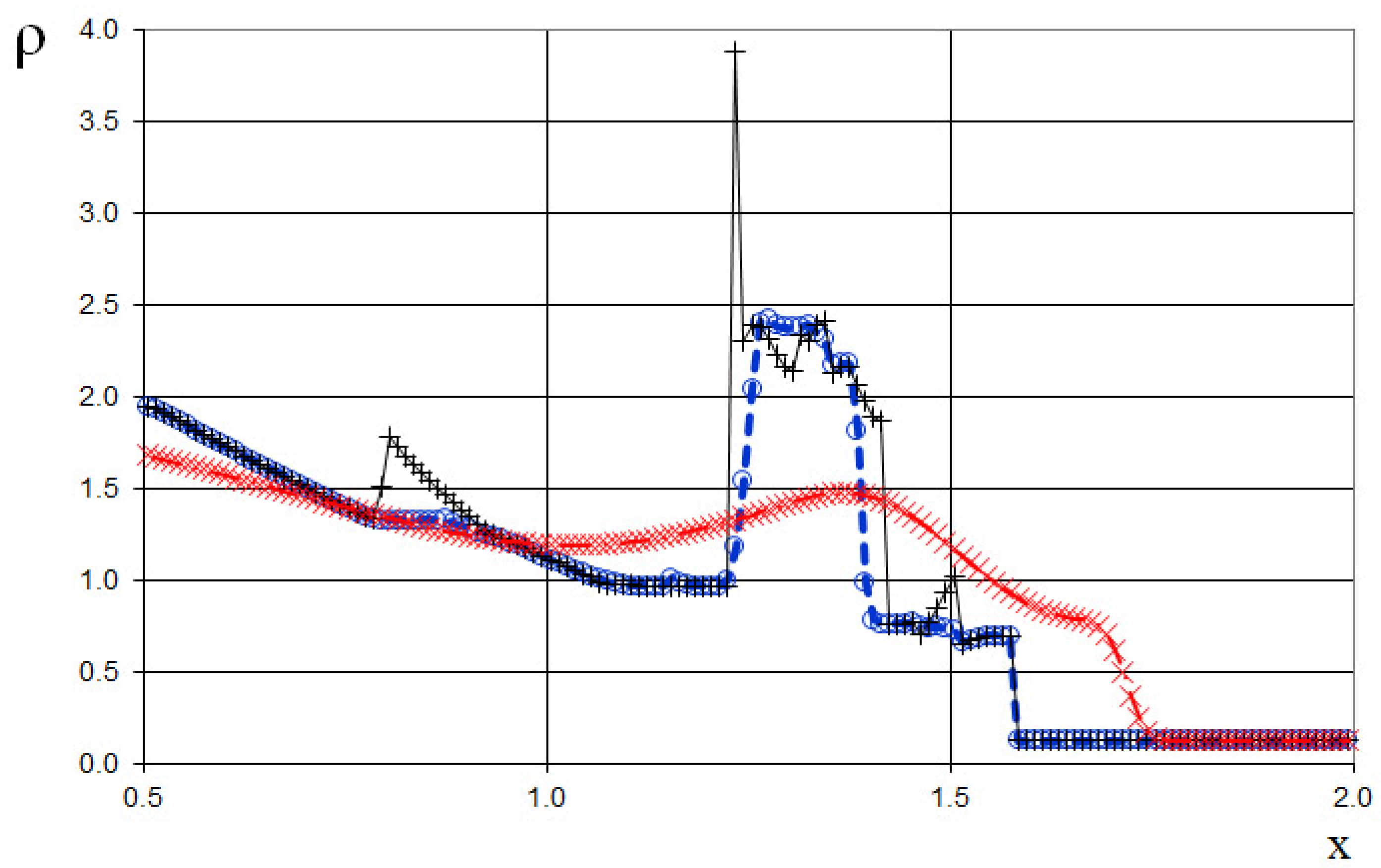
3.7. Seventh Test Problem

The seventh example is the interaction of two Riemann problems with the initial conditions given by (71).

$$\begin{gathered} {\mathrm{p}}_{\mathrm{j}}^0=100, {\mathrm{u}}_{\mathrm{j}}^0=0, {\rho }_{\mathrm{j}}^0=5, \mathrm{if} {\mathrm{x}}_{\mathrm{j}}<0, \\ {\mathrm{p}}_{\mathrm{j}}^0=1, {\mathrm{u}}_{\mathrm{j}}^0=0, {\rho }_{\mathrm{j}}^0=1, \mathrm{if} 0\le {\mathrm{x}}_{\mathrm{j}}<0.4, \\ {\mathrm{p}}_{\mathrm{j}}^0=0.1, {\mathrm{u}}_{\mathrm{j}}^0=0, {\rho }_{\mathrm{j}}^0=0.125, \mathrm{if} {\mathrm{x}}_{\mathrm{j}}\ge 0.4. \end{gathered}$$

(71)

Also, this is a more complicated problem proposed by Sod [27] (second and third lines of the formula), to which another discontinuity decay (stronger than in (70)) was added (using the first line of the Formula (71)).

The modeling region was defined as $\mathrm{x}\in \left[-2; 2\right]$. The grid consisted of 400 cells, with a grid spacing of $\mathrm{h}=0.01$. The time step for the acoustics stage was determined based on the Courant criterion (15), with ${\mathrm{k}}_{\mathrm{c}}=3$, meaning the shock spreads through three grid cells during this stage. The time step for the convection stage was determined based on Equation (17), with ${\mathrm{k}}_{\mathrm{u}}=11$, indicating that the shock spreads through eleven grid cells during this stage. The marching time step was set to ${}_{\Delta }\mathrm{t}=0.0236$. The acoustics and convection stages were executed during each marching time step, i.e., ${}_{\Delta }\mathrm{t}_{\mathrm{c}}={}_{\Delta }\mathrm{t}_{\mathrm{u}}={}_{\Delta }\mathrm{t}$.

The results are presented in Figure 34, Figure 35, Figure 36, Figure 37, Figure 38 and Figure 39, comparing the proposed method with the previous approach [24] and the data obtained by Harten [3] using the ULT1C scheme at $\mathrm{t}=0.2124$. The proposed scheme allows us to obtain more universal and accurate results than the previous method [24] and it has no sawtooth oscillations (dashed blue line), while the TVD scheme shows strong numerical viscosity of the solution at the shock wave.

Figure 40, Figure 41, Figure 42, Figure 43, Figure 44, Figure 45, Figure 46, Figure 47 and Figure 48 present a comparison between the results obtained using the proposed method and those obtained with the ULT1C scheme on finer grids. In these figures, the ULT1C method demonstrates lower numerical viscosity at the shock wave compared to that observed on coarser grids.

A comparison of CPU time consumption between the new method and Harten’s ULT1C method [3] for the seventh problem is presented in

Table 3. Comparison of computational costs between the present method and the ULT1C scheme for the seventh problem.

Cells of the Grid	The ULT1C Scheme	The Present Method
400	0.625 s	0.735 s
4000	16 s	7 s
40,000	25 min 25 s	1 h 11 min 53 s

. The results show that, for the grid with 40,000 points, the proposed method incurs significantly higher computational costs compared to the ULT1C scheme. However, as illustrated in Figure 46, Figure 47 and Figure 48, the results obtained with the proposed method on a grid with only 400 points are comparable to those obtained with the ULT1C method on a grid with 40,000 points, and moreover, the proposed method exhibits no numerical viscosity at the shock. Additionally, the computational cost of the proposed method for the grid with 400 points is substantially lower than that of the ULT1C scheme for the grid with 40,000 points. Thus, the proposed method enables faster solution times by employing a much coarser grid compared to the ULT1C method.

4. Discussion

The numerical solutions for the aforementioned well-known test cases were compared with the exact solutions, data from Harten’s method, and the results of the author’s previous approach. The obtained results lead to the following conclusions:

(1)

The primary advantage of the proposed method over the well-known TVD, ENO, and WENO methods is the elimination of the numerical viscosity (diffusion) for shocks.

(2)

Over time, shocks or rarefaction waves may spread slightly slower or faster than in the exact solution. This discrepancy arises from rounding the wave front positions to the grid cell accuracy, a consequence of using a fixed homogeneous grid.

(3)

The proposed scheme allows us to obtain more universal and accurate results than the previous method [24], and it has no sawtooth oscillations.

(4)

Although, for most of the test cases considered, the proposed method exhibits a higher computational cost than the ULT1C method; when using grids of the same size, it achieves comparable solution accuracy on much coarser grids. Consequently, when accounting for the required grid resolution, the proposed method ultimately outperforms the ULT1C method in terms of overall computational cost.

The accuracy of the proposed method for handling flow discontinuities is determined by the iterative Godunov exact solver. In the calculations, an iteration termination criterion of less than 10⁻⁵ is used to ensure convergence by measuring the pressure difference between consecutive iterations.

The directions for further research are connected with one-dimensional, two-dimensional Sedov problem modeling and two-dimensional Riemann problem simulations.

References

1. von Neumann, J.; Richtmyer, R.D. A method for the numerical calculation of hydrodynamic shocks. J. Appl. Phys. 1950, 21, 232. [Google Scholar] [CrossRef]
2. Jameson, A. Analysis and design of numerical schemes for gas dynamics, 1: Artificial diffusion, upwind biasing, limiters and their effect on accuracy and multigrid convergence. Int. J. Comput. Fluid Dyn. 1994, 4, 171–218. [Google Scholar] [CrossRef]
3. Harten, A. A high resolution scheme for the computation of weak solutions of hyperbolic conservation laws. J. Comput. Phys. 1983, 49, 357–393. [Google Scholar] [CrossRef]
4. Harten, A.; Engquist, B.; Osher, S.; Chakravarthy, S.R. Uniform high order accurate essentially non-oscillatory schemes, III. J. Comput. Phys. 1987, 71, 231–303. [Google Scholar] [CrossRef]
5. Liu, X.D.; Osher, S.; Chan, T. Weighted essentially non-oscillatory schemes. J. Comput. Phys. 1994, 115, 200–212. [Google Scholar] [CrossRef]
6. Harten, A. ENO schemes with subcell resolution. J. Comput. Phys. 1987, 83, 148–184. [Google Scholar] [CrossRef]
7. Harten, A.; Osher, S. Uniformly high order essentially non-oscillatory schemes I. SIAM J. Numer. Anal. 1987, 24, 279–309. [Google Scholar] [CrossRef]
8. Harten, A.; Osher, S.; Engquist, B.; Chakravarthy, S. Some results on uniformly high order accurate essentially non-oscillatory schemes. Appl. Numer. Math. 1986, 2, 347–377. [Google Scholar] [CrossRef]
9. Shu, C.-W.; Osher, S. Efficient implementation of essentially non-oscillatory shock-capturing schemes. J. Comput. Phys. 1988, 77, 439–471. [Google Scholar] [CrossRef]
10. Shu, C.-W.; Osher, S. Efficient implementation of essentially non-oscillatory shock-capturing schemes II. J. Comput. Phys. 1989, 83, 32–78. [Google Scholar] [CrossRef]
11. Jiang, G.-S.; Shu, C.-W. Efficient implementation of Weighted ENO schemes. J. Comput. Phys. 1996, 126, 202–228. [Google Scholar] [CrossRef]
12. Pawar, S.; San, O. CFD Julia: A Learning Module Structuring an Introductory Course on Computational Fluid Dynamics. Fluids 2019, 4, 159. [Google Scholar] [CrossRef]
13. Roe, P.L. Approximate Riemann solvers, parameter vectors, and difference schemes. J. Comput. Phys. 1997, 135, 250–258. [Google Scholar] [CrossRef]
14. Godunov, S.K. A difference scheme for numerical computation of discontinuous solution of hyperbolic equation. Mat. Sb. 1959, 47, 271–306. [Google Scholar]
15. LeVeque, R.J. Balancing source terms and flux gradients on high-resolution Godunov methods: The quasi-steady wave-propagation algorithm. J. Comput. Phys. 1998, 146, 346–365. [Google Scholar] [CrossRef]
16. Einfeldt, B. On Godunov-type methods for gas dynamics. SIAM J. Numer. Anal. 1988, 25, 294–318. [Google Scholar] [CrossRef]
17. Wu, Y.Y.; Cheung, K.F. Explicit solution to the exact Riemann problem and application in nonlinear shallow-water equations. Int. J. Numer. Meth. Fluids 2008, 57, 1649–1668. [Google Scholar] [CrossRef]
18. Kornev, N.; Denev, J.; Samarbakhsh, S. Theoretical Background of the Hybrid V?LES Method for Flows with Variable Transport Properties. Fluids 2020, 5, 45. [Google Scholar] [CrossRef]
19. Gadde, S.N.; Stieren, A.; Stevens, R.J.A.M. Large-Eddy Simulations of Stratified Atmospheric Boundary Layers: Comparison of Different Subgrid Models. Bound.-Layer Meteorol. 2021, 178, 363–382. [Google Scholar] [CrossRef]
20. Spalart, P.R.; Allmaras, S.R. A one-equation turbulence model for aerodynamic flows. AIAA Paper. 1992, 92, 0439. [Google Scholar]
21. Edeling, W.N.; Cinnella, P.; Dwight, R.P.; Bijl, H. Bayesian estimates of parameter variability in thek−εturbulence model. J. Comput. Phys. 2014, 258, 73–94. [Google Scholar] [CrossRef]
22. Yang, M.; Guo, M.; Zhang, Y.; Tian, Y.; Yi, M.; Le, J.; Zhang, H. Uncertainty quantification and identification of SST turbulence model parameters based on Bayesian optimization algorithm in supersonic flow. Int. J. Numer. Meth. Fluids 2024, 96, 277–296. [Google Scholar] [CrossRef]
23. Basiri, S.; Ghoreishi, S.M.; Safdari, J.; Yousefi-Nasab, S. Three-dimensional simulation of gas flow for predicting the pressure and velocity profiles inside a gas centrifuge machine using the DSMC method. Vacuum 2024, 219, 112664. [Google Scholar] [CrossRef]
24. Nikonov, V.A. Semi-Lagrangian Godunov-Type Method without Numerical Viscosity for Shocks. Fluids 2022, 7, 16. [Google Scholar] [CrossRef]
25. Taylor, E.M.; Wu, M.; Martin, M.P. Optimization of Nonlinear Error for Weighted Essentially Non-Oscillatory Methods in Direct Numerical Simulations of Compressible Turbulence. J. Comput. Phys. 2007, 223, 384–397. [Google Scholar] [CrossRef]
26. Toro, F.E. Riemann Solvers and Numerical Methods for Fluid Dynamics; Springer: Berlin/Heidelberg, Germany, 2009; ISBN 3-540-65966-8. [Google Scholar]
27. Sod, G.A. A survey of several finite difference methods for systems of nonlinear hyperbolic conservation laws. J. Comput. Phys. 1978, 107, 1–31. [Google Scholar] [CrossRef]
28. Lax, P.D. Weak solutions of nonlinear hyperbolic equations and their numerical computation. Commun. Pure Appl. Math. 1954, 7, 159–193. [Google Scholar] [CrossRef]
29. Carmouze, Q.; Saurel, R.; Chiapolino, A.; Lapebie, E. Riemann solver with internal reconstruction (RSIR) for compressible single-phase and non-equilibrium two-phase flows. J. Comput. Phys. 2020, 408, 109–176. [Google Scholar] [CrossRef]
30. Feng, H.; Hu, F.; Wang, R. A New Mapped Weighted Essentially Non-oscillatory Scheme. J. Sci. Comput. 2012, 51, 449–473. [Google Scholar] [CrossRef]
31. Fu, L.; Xiangyu, Y.H.; Nikolaus, A.A. A new class of adaptive high-order targeted ENO schemes for hyperbolic conservation laws. J. Comput. Phys. 2018, 374, 724–751. [Google Scholar] [CrossRef]
Figure 1. Algorithm for the acoustic stage.
Fluids 10 00133 g001
Figure 2. Initial conditions prior to solving the three Riemann problems.
Fluids 10 00133 g002
Figure 3. The first Riemann problem.
Fluids 10 00133 g003
Figure 4. The second Riemann problem.
Fluids 10 00133 g004
Figure 5. The third Riemann problem.
Fluids 10 00133 g005
Figure 6. Algorithm for the convection stage.
Fluids 10 00133 g006
Figure 7. Density plot for the shock-tube problem of Sod: the exact solution (line), the previous method [24] (red cross), and the present method (blue circle).
Fluids 10 00133 g007
Figure 8. Velocity plot for the shock-tube problem of Sod: the exact solution (line), the previous method [24] (red cross), and the present method (blue circle).
Fluids 10 00133 g008
Figure 9. Pressure plot for the shock-tube problem of Sod: the exact solution (line), the previous method [24] (red cross), and the present method (blue circle).
Fluids 10 00133 g009
Figure 10. Density plot for the Riemann problem of Lax: the exact solution (line), the previous method [24] (red cross), and the present method (blue circle).
Fluids 10 00133 g010
Figure 11. Velocity plot for the Riemann problem of Lax: the exact solution (line), the previous method [24] (red cross), and the present method (blue circle).
Fluids 10 00133 g011
Figure 12. Pressure plot for the Riemann problem of Lax: the exact solution (line), the previous method [24] (red cross), and the present method (blue circle).
Fluids 10 00133 g012
Figure 13. Density plot for the Riemann problem of Lax: the exact solution (line) and the present method (blue circle).
Fluids 10 00133 g013
Figure 14. Velocity plot for the Riemann problem of Lax: the exact solution (line) and the present method (blue circle).
Fluids 10 00133 g014
Figure 15. Pressure plot for the Riemann problem of Lax: the exact solution (line), and the present method (blue circle).
Fluids 10 00133 g015
Figure 16. Density plot for the Shu–Osher shock-tube problem (67), using the coarse grid (192 grid points): the “exact” solution [25] (line), the previous method [24] (cross), and the present method (circle).
Fluids 10 00133 g016
Figure 17. Density plot for the Shu–Osher shock-tube problem, using the fine grid (384 grid points): the “exact” solution [25] (line), the previous method [24] (red cross), and the present method (blue circle).
Fluids 10 00133 g017
Figure 18. Density plot for the Shu–Osher shock-tube problem, using the finer grid (1000 grid points): the “exact” solution [25] (line), the previous method [24] (cross), and the present method (circle).
Fluids 10 00133 g018
Figure 19. Density plot for the double expansion wave problem (68) for the one-dimensional scalar hyperbolic conservation law, using the coarse grid (100 grid points): the exact solution [29] (line), the author’s previous work method [24] (red cross), and the present method (blue circle).
Fluids 10 00133 g019
Figure 20. Velocity plot for the double expansion wave problem (68) for the one-dimensional scalar hyperbolic conservation law, using the coarse grid (100 grid points): the exact solution [29] (line), the author’s previous work method [24] (red cross), and the present method (blue circle).
Fluids 10 00133 g020
Figure 21. Pressure plot for the double expansion wave problem (68) for the one-dimensional scalar hyperbolic conservation law, using the coarse grid (100 grid points): the exact solution [29] (line), the author’s previous work method [24] (red cross), and the present method (blue circle).
Fluids 10 00133 g021
Figure 22. Density plot for the double expansion wave problem (68) for the one-dimensional scalar hyperbolic conservation law, using the finer grid (1000 grid points): the exact solution [29] (black solid line), the author’s previous work method [24] (red dotted line), and the present method (blue dashed line).
Fluids 10 00133 g022
Figure 23. Velocity plot for the double expansion wave problem (68) for the one-dimensional scalar hyperbolic conservation law, using the finer grid (1000 grid points): the exact solution [29] (black solid line), the author’s previous work method [24] (red dotted line), and the present method (blue dashed line).
Fluids 10 00133 g023
Figure 24. Pressure plot for the double expansion wave problem (68) for the one-dimensional scalar hyperbolic conservation law, using the finer grid (1000 grid points): the exact solution [29] (black solid line), the author’s previous work method [24] (red dotted line), and the present method (blue dashed line).
Fluids 10 00133 g024
Figure 25. Density plot for the problem (69): the exact solution (line), the previous method [24] (cross), and the present method (circle).
Fluids 10 00133 g025
Figure 26. Velocity plot for the problem (69): the exact solution (line), the previous method [24] (cross), and the present method (circle).
Fluids 10 00133 g026
Figure 27. Pressure plot for the problem (69): the exact solution (line), the previous method [24] (cross), and the present method (circle).
Fluids 10 00133 g027
Figure 28. Density plot for the two Riemann problems interaction (70): the ULT1C scheme of Harten (red dash dotted line), the previous method [24] (black solid line), and the present method (blue dashed line).
Fluids 10 00133 g028
Figure 29. Magnified view of density plot for the two Riemann problems interaction (70): the ULT1C scheme of Harten (red dash dotted line), the previous method [24] (black solid line), and the present method (blue dashed line). Blue circles, red crosses and black crosses are indicating grid points.
Fluids 10 00133 g029
Figure 30. Velocity plot for the two Riemann problems interaction (70): the ULT1C scheme of Harten (red dash dotted line), the previous method [24] (black solid line), and the present method (blue dashed line).
Fluids 10 00133 g030
Figure 31. Magnified view of velocity plot for the two Riemann problems interaction (70): the ULT1C scheme of Harten (red dash dotted line), the previous method [24] (black solid line), and the present method (blue dashed line). Blue circles, red crosses and black crosses are indicating grid points.
Fluids 10 00133 g031
Figure 32. Pressure plot for the two Riemann problems interaction (70): the ULT1C scheme of Harten (red dash dotted line), the previous method [24] (black solid line), and the present method (blue dashed line).
Fluids 10 00133 g032
Figure 33. Magnified view of pressure plot for the two Riemann problems interaction (70): the ULT1C scheme of Harten (red dash dotted line), the previous method [24] (black solid line), and the present method (blue dashed line). Blue circles, red crosses and black crosses are indicating grid points.
Fluids 10 00133 g033
Figure 34. Density plot for the two Riemann problems interaction (71): the ULT1C scheme of Harten (red dash dotted line), the previous method [24] (black solid line), and the present method (blue dashed line).
Fluids 10 00133 g034
Figure 35. Magnified view of density plot for the two Riemann problems interaction (71): the ULT1C scheme of Harten (red dash dotted line), the previous method [24] (black solid line), and the present method (blue dashed line). Blue circles, red crosses and black crosses are indicating grid points.
Fluids 10 00133 g035
Figure 36. Velocity plot for the two Riemann problems interaction (71): the ULT1C scheme of Harten (red dash dotted line), the previous method [24] (black solid line), and the present method (blue dashed line).
Fluids 10 00133 g036
Figure 37. Magnified view of velocity plot for the two Riemann problems interaction (71): the ULT1C scheme of Harten (red dash dotted line), the previous method [24] (black solid line), and the present method (blue dashed line). Blue circles, red crosses and black crosses are indicating grid points.
Fluids 10 00133 g037
Figure 38. Pressure plot for the two Riemann problems interaction (71): the ULT1C scheme of Harten (red dash dotted line), the previous method [24] (black solid line), and the present method (blue dashed line).
Fluids 10 00133 g038
Figure 39. Magnified view of pressure plot for the two Riemann problems interaction (71): the ULT1C scheme of Harten (red dash dotted line), the previous method [24] (black solid line), and the present method (blue dashed line). Blue circles, red crosses and black crosses are indicating grid points.
Fluids 10 00133 g039
Figure 40. Density plot for the two Riemann problems interaction (71) (4000 grid points): the ULT1C scheme of Harten (red dash dotted line) and the present method (blue dashed line).
Fluids 10 00133 g040
Figure 41. Velocity plot for the two Riemann problems interaction (71) (4000 grid points): the ULT1C scheme of Harten (red dash dotted line) and the present method (blue dashed line).
Fluids 10 00133 g041
Figure 42. Pressure plot for the two Riemann problems interaction (71) (4000 grid points): the ULT1C scheme of Harten (red dash dotted line) and the present method (blue dashed line).
Fluids 10 00133 g042
Figure 43. Density plot for the two Riemann problems interaction (71) (40,000 grid points): the ULT1C scheme of Harten (red dash dotted line) and the present method (blue dashed line).
Fluids 10 00133 g043
Figure 44. Velocity plot for the two Riemann problems interaction (71) (40,000 grid points): the ULT1C scheme of Harten (red dash dotted line) and the present method (blue dashed line).
Fluids 10 00133 g044
Figure 45. Pressure plot for the two Riemann problems interaction (71) (40,000 grid points): the ULT1C scheme of Harten (red dash dotted line) and the present method (blue dashed line).
Fluids 10 00133 g045
Figure 46. Density plot for the two Riemann problems interaction (71): the ULT1C scheme of Harten (red dash dotted line) (40,000 grid points) and the present method (blue dashed line) (400 grid points).
Fluids 10 00133 g046
Figure 47. Velocity plot for the two Riemann problems interaction (71): the ULT1C scheme of Harten (red dash dotted line) (40,000 grid points) and the present method (blue dashed line) (400 grid points).
Fluids 10 00133 g047
Figure 48. Pressure plot for the two Riemann problems interaction (71): the ULT1C scheme of Harten (red dash dotted line) (40,000 grid points) and the present method (blue dashed line) (400 grid points).
Fluids 10 00133 g048