Numerical Mixing Index: Definition and Application on Concrete Mixer

Abstract

In this work, a statistical method is applied to a multiphase CFD simulation of concrete mixing performed in a truck mixer. The numerical model is based on an Eulerian–Eulerian approach in a transient regime. The aggregate materials are simulated as dispersed solid particles of various diameters, while the cement paste is simulated as a non-Newtonian continuous fluid. The first ten drum revolutions are analyzed from the condition of the completely segregated materials. The cell mixing index, defined by a statistical method in terms of mean, variance, and density probability function, is applied to the analysis of the simulation results. The statistical variables are implemented using the fluid dynamics code in the post-processing result analyses. The method predicts the distribution efficiency of the materials within a truck mixer as a function of its internal geometry, rotation speed, and mixture composition. As the number of revolutions increases, the distribution qualitatively improves, as shown by the motion fields, velocities, and vortices of the various materials, quantified through the calculation of the mixing index. The illustrated method can be used to predictively calculate the distribution effectiveness of new truck mixer designs before prototyping them and can be applied to other types of mixers. Furthermore, this study can be applied to liquid–solid mixing processes analyzed via the Eulerian multiphase numerical approach.

1. Introduction

In recent years, the coupling of the Discrete Element Method (DEM) and Computational Fluid Dynamics (CFD) has gained significant attention in the scientific community due to its ability to model complex particle–fluid interactions with high accuracy. Numerous studies [1,2,3,4] have demonstrated the effectiveness of DEM-CFD applications in various fields, including granular flow and bonded agglomerates. The process of homogenization, understood as the mixing of segregated materials, has been extensively studied to achieve uniformity, to ensure consistency in numerical simulations, and to optimize processes in various industries [5,6,7,8].

Nevertheless, the calibration of numerical models remains a critical aspect of ensuring their accuracy and reliability. Recent advancements in calibration methods have shown promise in improving model predictions by optimizing parameter settings [2,9,10,11,12,13].

An analysis of the literature [14,15,16,17] shows that one of the methods for a quantitative analysis of the mixing of several components, regardless of their phase and the mixing method used, is a statistical method. The method in question involves the mathematical quantification of the distribution of the concentrations of the different elements in a certain volume sample of the mixture.

In order to evaluate the distribution of concentrations, the statistical parameters used are the mean and the standard deviation, with the latter calculated as the square root of the variance. This method is versatile, as it makes it possible to analyze the mixing either experimentally, by taking an arbitrary number of samples from the mixture, or numerically, by analyzing the distribution of components in certain points in the simulated fluid domain.

In statistics, according to Equation (1), the sample mean of a quantity X over a sample number n is defined as follows:

$$\overline{X}={\displaystyle \frac{\sum _{j=1}^n{X}_j}{n}}$$

(1)

The sample standard deviation S is defined according to Equation (2):

$$S=\sqrt{{\displaystyle \frac{{\sum _{j=1}^n{(X}_j-\overline{X})}^2}{n-1}}}$$

(2)

The two parameters, when applied to the concentration of a component on n samples, allow us to assess whether the mixing has occurred homogeneously or if the components have been segregated.

For a mixture, the Lacey mixing index can be defined [18] on the basis of Equation (3):

$$M_L={\displaystyle \frac{{S_0}^2-S^2}{{S_0}^2-{S_R}^2}}$$

(3)

where S₀ is the standard deviation for complete segregation and S_R is the standard deviation for optimal mixing. As it is defined, Lacey’s index is a number between 0 and 1 and can be understood as the ratio between the actual extent of the mixing and the ideal optimal limit to which the mixing can tend [19].

Similarly, by omitting the segregation term S₀ from Equation (3), the index can be simplified, obtaining Equation (4):

$$M_L={\displaystyle \frac{S^2}{{S_R}^2}}$$

(4)

In this definition, mixing can be called optimal to the extent that the value of M is close to one, admitting values greater than one as well.

The standard deviation method has been successfully employed by various authors for the study of simulated liquid–solid suspensions by a multiphase CFD approach [20,21,22]. The increased homogenization (improved suspension quality) results in a reduction in the standard deviation. Ref. [23] presented a method based on the distribution, mean, and standard deviation of the velocity magnitude, a method which can be easily applied in the comparison of various velocity profiles from CFD simulations. In other words, the Lacey mixing index and standard deviation are the most commonly used methods and are well suited to the problem. These methods are not only widely recognized but also simple to apply. CFD simulation can be an excellent and cost-effective tool to calculate mixing efficiency using CFD simulators, even with complex impeller geometries [24]. Ref. [25] defined a new mixing index for measuring the efficiency of a Twin Screw Extruder; the CFD simulation was validated by a comparison with the experimental data.

Regarding the study of concrete mixing by numerical means, CFD models can be used for the simulation of a truck mixer [26], a paddle and screw mixer for cement [27], and a cement slurry mixer [28]. However, in these studies, the mixing index and overall quality of mixing were not calculated, and the fluid was considered homogeneous. Instead, in the current study, the mixing of the phases—water, cement, sand, and gravel—is taken into account by calculating the volumetric fractions of each component. As shown above, the calculation of the mixing index by means of a statistical method has not yet been applied to concrete mixing that has been investigated using an Eulerian computational approach. There are few works in the literature on the simulation of concrete mixing, and the DEM approach is used in all of them. This approach can be difficult to apply, especially in dense flows with non-Newtonian dynamics where the motion is governed by viscous effects, which occur in cement paste and concrete dynamics. The advantage of the DEM approach is that the mixing index is easily calculated. On the contrary, the study of mixers for concrete with an Eulerian multiphase CFD approach can lead to a more accurate result on the viscous and non-Newtonian dynamics of the mixture (cement paste or concrete); however, but it would be complicated to apply the concept of a mixing index. In other words, it is difficult to estimate how well the flow is mixed with an index.

In recent years, we have focused on the study of fresh concrete dynamics in a concrete mixer via multiphase CFD methods. In the work by [29], a CFD model was presented that simulated the discharge of fresh concrete from a concrete mixer; the flow characteristics of the model were calibrated with experimental tests in the field. In the work by the same authors [30] issued within the following year, however, the same model was used to predict the capacity level of a concrete mixer as a function of the consistency class of the concrete. In both of these works, fresh concrete was simulated as the Bingham fluid, and they focused on studying the dynamics of the fresh concrete just produced, while the mixing process was not addressed. Instead, in [31], a multiphase Eulerian model was developed in a transient regime, which was useful for studying the concrete mixing process inside a truck concrete drum mixer. For the first time, the model simulated the distribution of the four phases (air, cement paste, gravel, and sand) inside the mixer as the number of revolutions of the rotating drum increased. In this work, the model was validated and some fluid dynamic parameters characteristic of the mixing process, which were previously unknown, were calculated. However, the work lacked a method for the quantitative calculation of the mixing of the various phases.

In this paper, we illustrate a methodology focusing on the definition and calculation of the numerical mixing index through the implementation of some statistical variables in the commercial fluid dynamics code used for the computation. Through the model and the application of the mixing index calculation, as carried out in this work, it is possible to optimize the geometry and operating parameters such as rotation speed and inclination.

Before this work, the mixing index had never been applied to the study of concrete mixing simulated with a multi-phase CFD approach. The mixing efficiency of a truck mixer is currently evaluated indirectly, through the measurement of the absorbed torque or with other experimental methods; numerically, it is evaluated when the truck mixer is simulated with DEM approaches. The definition and application of the mixing index allow for the evaluation of the mixing process and its efficiency using a numerical Eulerian approach. When the mixer is studied numerically with an Eulerian method, without the cell mixing index, the evaluation of mixing quality would be impossible, necessitating a Lagrangian approach. The cell mixing index is the variable that enables the calculation of a multiphase mixing process when studied with a numerical Eulerian method.

This work makes it possible to quantify the efficiency of a concrete mixer through a universally adopted index, even when studied with a multiphase CFD approach, and can be applied to other types of solid–liquid mixers present in other fields such as process engineering or the chemical industry, which can be studied with the same approach.

2. Analyzed Machine

Off-road concrete mixer trucks are designed to produce homogeneous concrete mixtures directly at building sites. The inclination angle of the drum can vary from 15° to 20°; during the mixing process, this figure is kept at 18°. The maximum angular speed is 22 rpm, which is reached during the mixing phase. As the components are loaded into the drum, it starts revolving in one direction to permit mixing; once the mixing is complete, the mixture is discharged by reversing the speed direction. The drum has two double truncated cone sections, with different cone angles in the upper and lower parts, which are divided by a middle cylindrical section (Figure 1).

The raw materials are loaded using a water pump and a charging hopper for the solid aggregates. Generally, in the concrete production with batch mixers, it is possible to identify three different phases (

Table 1. Working cycle of a self-loading truck concrete mixer.

Phase	Time [s]	Volume [m3]
Charge material	30–320	0–1.35
Mixing	320–620	1.35
Discharge	620–700	1.35–0

). The first phase is the loading phase, which starts with a first hopper of gravel, followed by the addition of cement and water; afterwards, alternate loads of gravel and sand are added until the required mixture is obtained. Finally, an additional quantity of water is loaded in order to achieve the final concrete mix design. The second phase is the mixing phase, in which the cement paste, formed by water and cement, is absorbed by the inert materials, i.e., sand and gravel. This phase leads to the formation of agglomerates which subsequently dissolve, homogenizing the mixture. The third phase of the process is the discharge phase, which takes place once mixing has been completed. The mixture is discharged by reversing the direction, and the rotational velocity in this phase must be chosen carefully in order to speed up the cycle phase without causing segregation of the mixture, which would result in low-quality concrete. The mix design has to be chosen before loading the material, as it will determine the properties of the concrete.

The concrete mix design and the material loading order are presented in the following tables (

Table 2. Analyzed Mix Design.

Material	Mix Design [Weight %]
Water	7
Cement	13
Sand	38
Gravel	42

and

Table 3. Drum Loading Cycle.

Loading Order	Material	Weight [kg]
1st	Gravel	758
2nd	Cement	476
3rd	Water	149
4th	Gravel	758
5th	Sand	683
6th	Sand	683
7th	Water	99

). The presented mix design is the most commonly used one for the main applications of the machine under investigation.

3. Multiphase Model of the Mixing

3.1. Governing Equations

The numerical simulations were carried out with the commercial CFD code ANSYS CFX 19.2 [32]. This code solved the 3D Reynolds-averaged form of the Navier–Stokes equations by using a finite element approach based on a finite volume method. A second-order high-resolution advection scheme was adopted to calculate the advection terms in the discrete finite volume equations. An Eulerian inhomogeneous model with an interphase transfer particle approach was used for resolving the multiphase simulation. The governing equations are listed below:

$${\displaystyle \frac{\partial }{\partial t}}\left({\rho }_{\alpha }{r}_{\alpha }\right)+\nabla ·\left({\rho }_{\alpha }{r}_{\alpha }{U}_{\alpha }\right)=0$$

(5)

$${\displaystyle \frac{\partial }{\partial t}}\left({\rho }_{\alpha }{r}_{\alpha }{U}_{\alpha }\right)+\nabla ·(r_{\alpha }{\rho }_{\alpha }{U}_{\alpha }⨂U_{\alpha })=-r_{\alpha }\nabla p_{\alpha }+\nabla ·(r_{\alpha }{\mu }_{\alpha }\left(\nabla U_{\alpha }+{\left[U_{\alpha }\right]}^T\right))+\sum _{\beta =1}^{N_P}{M}_{\alpha \beta }$$

(6)

$$\sum r_{\alpha }=1$$

(7)

These 17 (12 momentum, 4 phasic continuity, 1 volume fraction) nonlinear partial differential equations must be solved for the 17 dependent variables [(U_α, V_α, W_α), r_α, p], where subscript index α = 1, …, 4 identifies the phase. For the other characteristics of the multiphase model (i.e., Continuous–Dispersed, Continuous–Continuous, and Dispersed–Dispersed iterations), see [31].

3.2. Geometry and Mesh

The 3D CAD geometry was imported into a commercial meshing software program, ANSYS ICEM CFD 19.2 [33]. The discretization of the fluid domain was obtained using a mesh made up of hexahedral elements in order to increase the numerical accuracy and decrease the time and effort needed for the simulations. The generation of hexahedral elements needed a specific blocking construction, associating the vertex, edges, and faces of the blocks to the points, curves, and surfaces inside the geometrical domain. A mesh with uniform element density must be generated to achieve a consistent element size distribution throughout the entire internal drum geometry.

For the grid sensitivity test, the following three tetrahedral element grids were generated: Mesh 1, comprising 3.8 × 10⁶ elements; Mesh 2, comprising 4.8 × 10⁶ elements; and Mesh 3, comprising 6.8 × 10⁶ elements. Examples of the meshes obtained are shown in Figure 2a,b.

3.3. Boundary Conditions

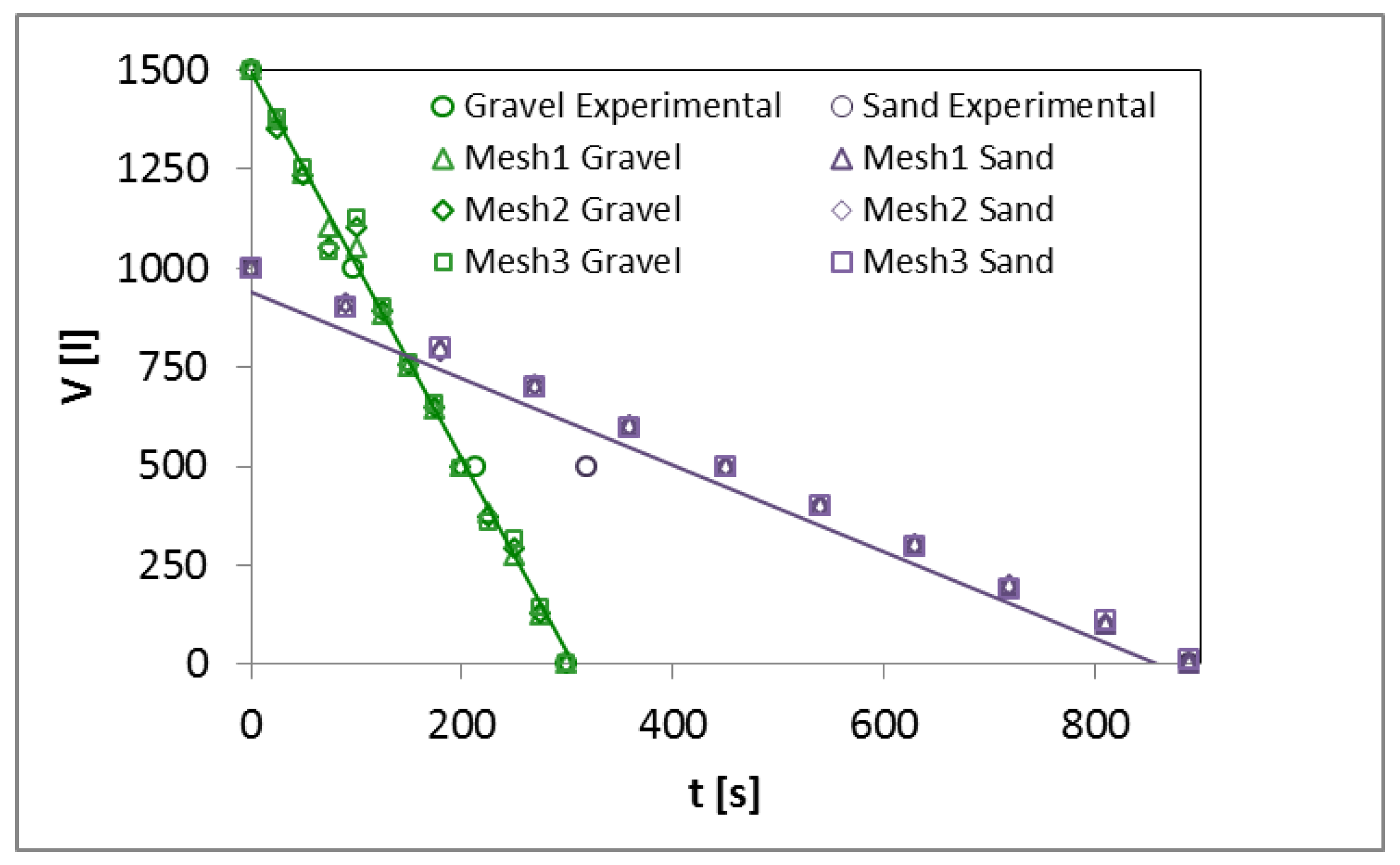
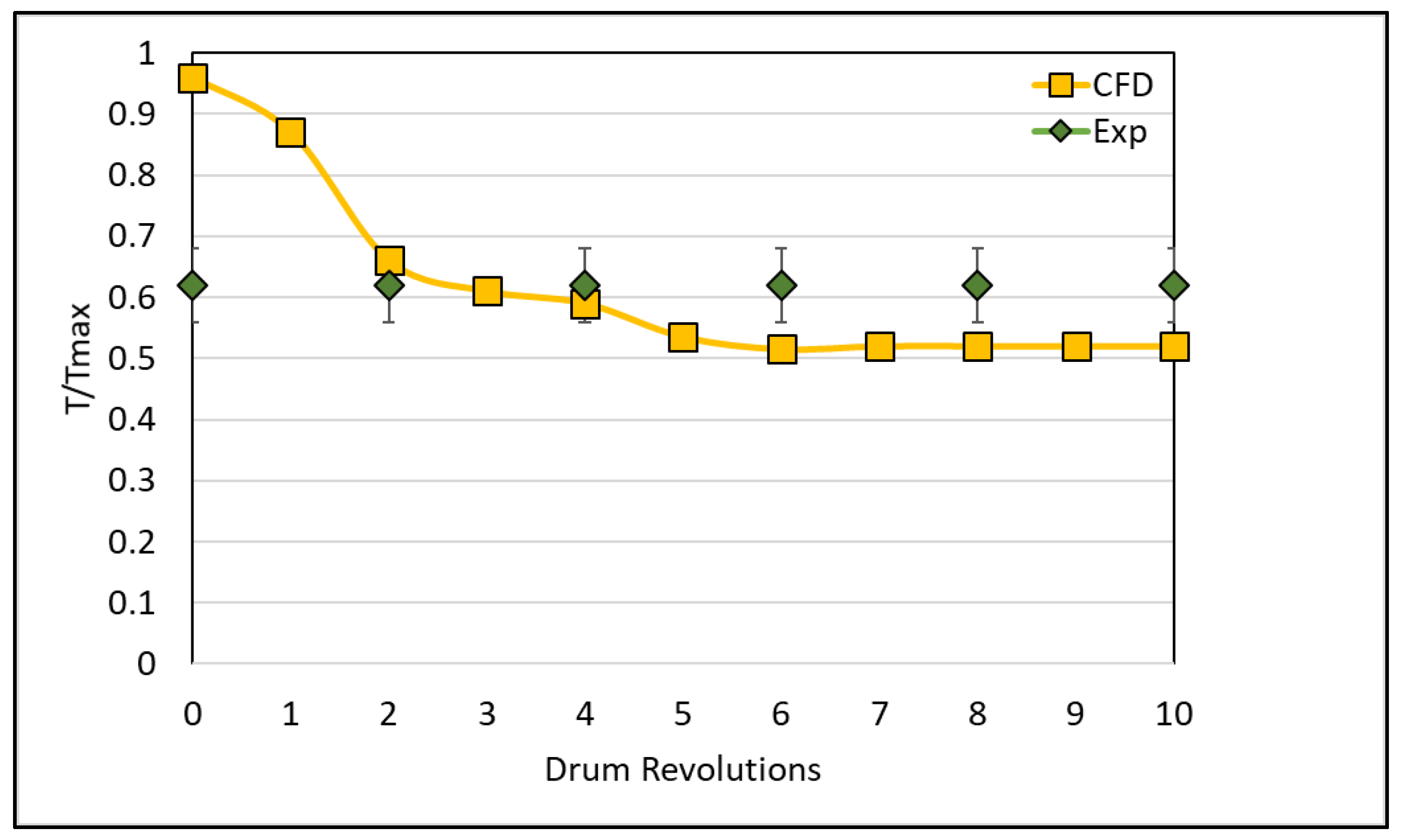
All the phases are completely segregated and stratified at the start of the simulation. Gravel is placed on the bottom, sand is placed between gravel and cement paste, and air is set to fill the remaining volume. Inside the domain, the buoyancy model is used by applying the gravitational force. In order to stabilize the initialization of the simulation, the static pressure gradient is set along the height of the drum, following Stevino’s law, as follows:

$$p\left(y\right)=\rho gy+p_{atm}$$

(8)

The parameters imposed for each species are shown in

Table 4. Material parameters used.

	Air	Cement Paste	Sand	Gravel
fluid scheme	continuous fluid	continuous fluid	dispersed solid	dispersed solid
ρ [kg/m3]	1.2	1283	2560	2650
viscosity model	Newtonian	Bingham	-	-
particle diameter [mm]	-	-	2	20
maximum packing			0.62	0.62
volume fraction	-	0.2	0.38	0.42
turbulence model	laminar	laminar	-	-

. Some additional parameters are the air at atmospheric pressure, 22 rpm for a constant drum rotational speed, and a free slip wall boundary condition for every wall boundary set.

According to the literature [34], cement paste can be considered a Bingham fluid with the appropriate yield stress and plastic viscosity, i.e., τ₀ and K, respectively.

$$\eta ={\displaystyle \frac{{\mathsf{\tau }}_0}{\stackrel{·}{\mathsf{\gamma }}}}+\mathrm{K}$$

(9)

where η is the apparent viscosity and γ is the shear rate. The plastic viscosity depends largely on the concentration of cement and the yield stress as a function of hydration time. From the mix design used (Table 2), the water/cement ratio is about 0.5; at this value, the yield stress is equal to 0.7 Ncm and the plastic viscosity is set to 0.5. Portland Cement with ρ_c = 1506 kg/m³ was used; consequently, with the weights reported in Table 3, it is possible to calculate the density of cement paste.

A surface tension coefficient σ between air and concrete is set to 66 mN/m [35]. This value is applied in the continuum surface force model of [36], which is used in the CFX 19.2 software to calculate the effect of surface tension in the Cauchy moment equation. Every wall is modeled as an ideal No Slip smooth wall in order to avoid the effect of wall roughness on the results.

The transient analysis convergence is controlled by setting an adaptive time step around 10⁻⁴:10⁻³ s, regulated by the RMS Courant number, which is set to 0.5. The convergence criteria on the equations’ residual values are set to 10⁻⁴. A second-order high-resolution advection scheme is implemented to compute the advection terms within the discrete finite volume equations. A trilinear interpolation technique is used to interpolate the values of pressure and velocity between the nodes of a three-dimensional grid. With these settings for the transient simulations, the global imbalances are normally kept below ±10%.

3.4. Validation

The model presented above was validated in several steps. The first validation was performed by comparing an experimental truck emptying over time with a computational drum emptying (Figure 3 and Figure 4). This made it possible to validate the cement paste viscosity model and the aggregates’ solid particle model used for numerical simulations. A grid independence analysis was conducted, and convergence was monitored both by keeping the imbalances within 10 percent, as mentioned above, and by analyzing the superficial velocity, which is a characteristic velocity used in multiphase flows [37].

This showed that the flow velocity could be considered convergent only after eight drum revolutions.

Finally, the torque absorbed by the machine during the actual mixing process was measured during an experimental test and later compared with the calculated torque from the full numerical model simulation (Figure 5).

P_mec = M_t ω

(10)

where M_t is the torque acting on the internal drum and blade surfaces, and ω is the rotational velocity.

The comparison is shown in Figure 5; as the model represents the first few minutes of the actual physical process, the torque curves are only compared for the first few revolutions.

4. Numerical Mixing Index

Application of the Mixing Index at the Concrete Mixing Multiphase Simulation

An Eulerian–Eulerian model was adopted for multiphase simulations, which reproduces the problem by defining the volume fractions of the various phases present in the domain elements.

Following this approach, the mixing index adopted for the mixing analyses is defined by Equation (11):

$$R_{i,n}={\displaystyle \frac{V_{i,n}}{V_{i,ref}}}$$

(11)

where R_i,n is defined as the mixing index of the i-th phase in the n-th element; V_i,n denotes the volume fraction of the i-th phase in the n-th element; and V_i,ref is the mix design volume fraction of the analyzed concrete. The mix design values for each phase are given in

Table 5. Calculation of design mix design.

Phase	Weight [kg]	Density [kg/m3]	Volume [m3]	Mix Design [%]
Cement paste	724	1700	0.426	28
Sand	1516	2660	0.570	37.4
Gravel	1366	2590	0.527	34.6

.

The R ratio calculated, as explained above, makes it possible to quantify if the volume fraction of each phase approximates the optimal design value over time for each domain element, as follows:

-

R < 1—insufficient concentration of the phase in the element;

-

R = 1—optimal concentration of the phase in the element;

-

R > 1—excessive concentration of the phase in the element.

The study of this parameter by static methods therefore allows us to evaluate the distribution of phases in the domain during drum rotation, under the assumption that the optimal design is given by a homogeneous distribution of the various phases according to the mix design. The two statistical parameters adopted for the study are mean and variance of R.

-

Mean of the mixing index:

Once the values of R in the domain have been calculated, the mean is averaged over the volume. The mix design calculation does not include the influence of air, which is present in the simulations performed. For this reason, to study the mean of R, the elements in the domain with a volume fraction of air equal to 1, i.e., all elements having only air inside, are excluded from the calculation.

For each i-th phase, at each instant of time, we can use Equation (12):

$$R_{m,i}={\displaystyle \frac{\sum _{j=1}^n{R}_{i,j}}{n}}$$

(12)

where n is the number of elements in the analyzed domain, considering the assumptions about the air phase distribution just highlighted. The value of R_m has the same trend as R, so for an optimal simulation, a value as close to one as possible should be aimed for with Equation (12).

-

Variance of the mixing index:

The variance of R is a parameter that indicates the dispersion of R around its mean value. For each i-th stage, at a given instant of time, the variance S² is calculated according to Equation (13):

$$S_i^2={\displaystyle \frac{{\sum _{j=1}^n{(R}_{i,j}-\overline{R_i})}^2}{n-1}}$$

(13)

In the ideal case of perfect mixing, S² should be equal to zero, indicating a configuration in which all the elements in the domain have a value of R equal to R_m.

The absolute value of S² is affected by the number of grid elements used; therefore, it is necessary to apply grid-independent conditions for the S² parameter as well. Figure 6 shows the trends of S² as the number of simulated revolutions increases for different numerical grids; two meshes have been tested with 1.5 × 10⁶ hexa elements and 5.0 × 10⁶ hexa elements. As the number of elements increases (more uniform grid), it can be observed that the variance curve is more linear.

-

Probability density function:

Once the steady-state values of R_m and S² are found for each phase, the resulting Gaussian probability distributions can be compared.

For the Gaussian distribution of a quantity with mean μ and variance σ², the probability density function f_(x) is calculated according to Equation (14):

$$f_{\left(x\right)}={\displaystyle \frac{1}{\sigma \sqrt{2\pi }}}{e}^{-{\displaystyle \frac{{(x-\mu )}^2}{{2\sigma }^2}}}$$

(14)

In an ideal case, in which Rm of each phase tends to 1 and S² tends to 0, the resulting Gaussian tends to a degenerate random variable in 1; meaning that, as the distribution of each phase improves, the Gaussian curve associated with the distribution of each phase in the domain should be increasingly closer and centered to 1.

-

Statistical definition implemented in the code:

Equations (11)–(13) are implemented via CEL (Cfx Expression Languages) in the fluid dynamics code. In particular, the expressions are as follows:

$$\begin{array}{l}\text{R<phase>=<phase>.Volume Fraction/MixDesign<phase>}\\ \text{Rm<phase>=ave(R<phase>)@VolumeComponent}\\ \text{S2<phase>=(sum((R<phase>-Rm<phase>)^2) @VolumeComponent)/((count()@VolumeComponent)-1)}\end{array}$$

where the quantity MixDesign<phase> indicates the reference volume fraction values given by Table 5, and the VolumeComponent is the computational domain in which the air volume fraction is less than 1.

5. Results

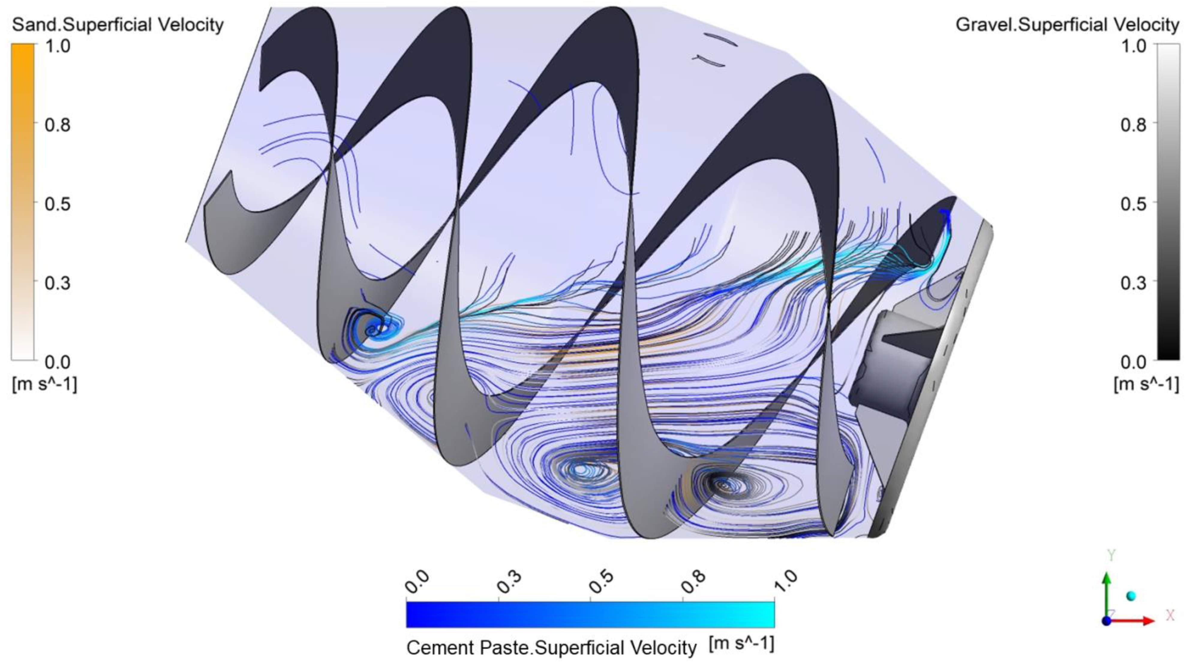
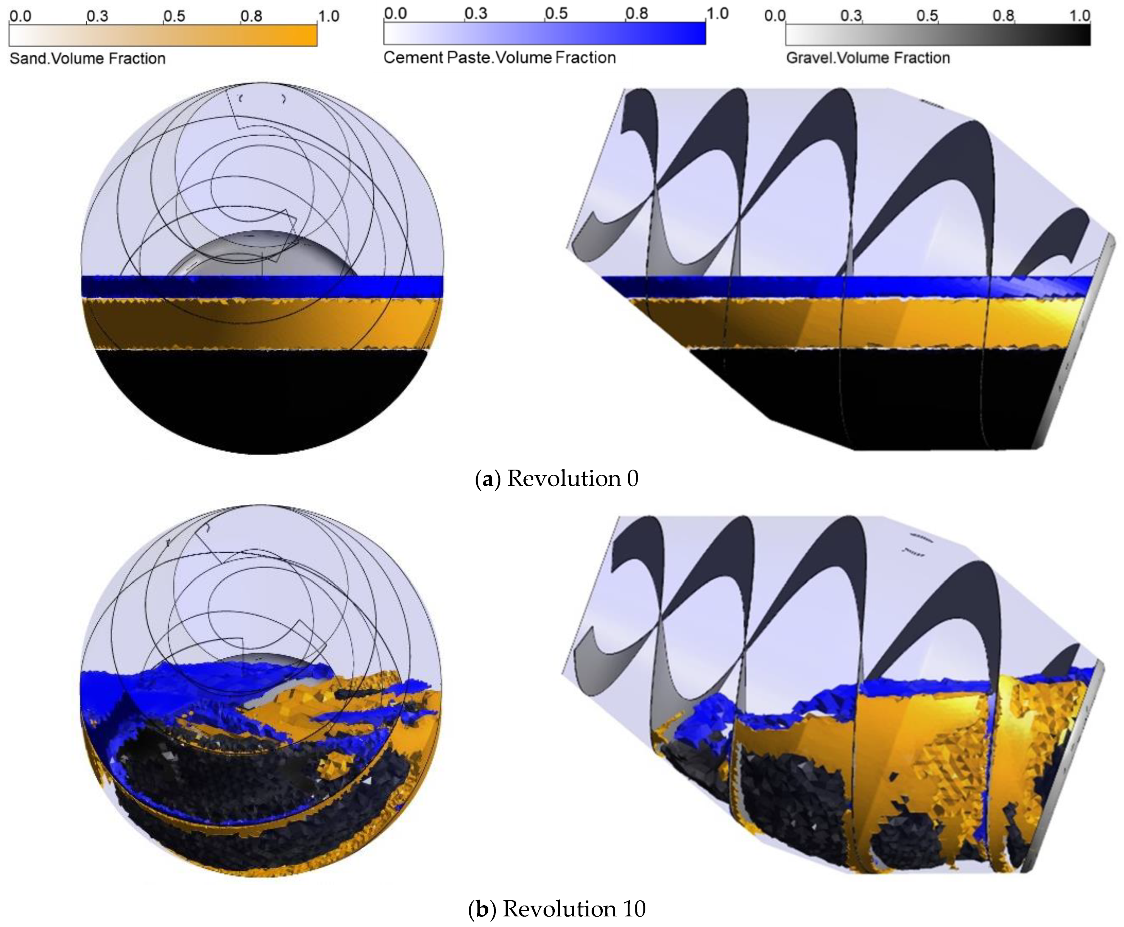
5.1. Motions of Mixing

In terms of the direction of flow motion, the streamlines of the various phases are shown in Figure 7. The motions of mixing are caused by two combined effects, with the first one being the mechanical action given by the rotation of the drum and simultaneously by the movement of the helixes, as well as the second one being given by the difference in density and species of the simulated phases. The combination of these two aspects results in a series of vortices that facilitate the dispersion of the phases.

5.2. Type of Mixing

Figure 8a,b show the phase concentrations in the initial condition and after 10 revolutions of the drum, respectively.

In Figure 8a, in the initial condition, the phases are fully segregated; the gravel is placed at the bottom of the mixer, the sand is placed in the middle, and the water is placed on top, in agreement with the initial condition set-up. After 10 revolutions (Figure 8b), the sand and gravel areas are approximately the same size, while the water areas are fewer and smaller, and most of the water remains on top. This is due to the transport and trail effects caused by the motion of the two-blade motion; in fact, their action, combined with the fact that the solid aggregates have a similar rheology, causes a mixing action along the helix profiles. This behavior is typical of the laminar mixing under high laminar stress [19,38]. The described behavior is justified by the quantity ratio (4:1) between the aggregates and the water.

5.3. Computation of Numerical Mixing Index

The values of the logarithmic tendency curves associated with the trend lines, calculated after 10 drum revolutions, were taken as the reference for R_m and S² for each phase. Once unique values of R_m and S² were found for each phase, the resulting Gaussian probability distributions could be compared.

By implementing the mean and variance values as the number of drum revolutions changes, the following trends can be derived (Figure 9 and Figure 10).

The following features are evident from the graphs:

-

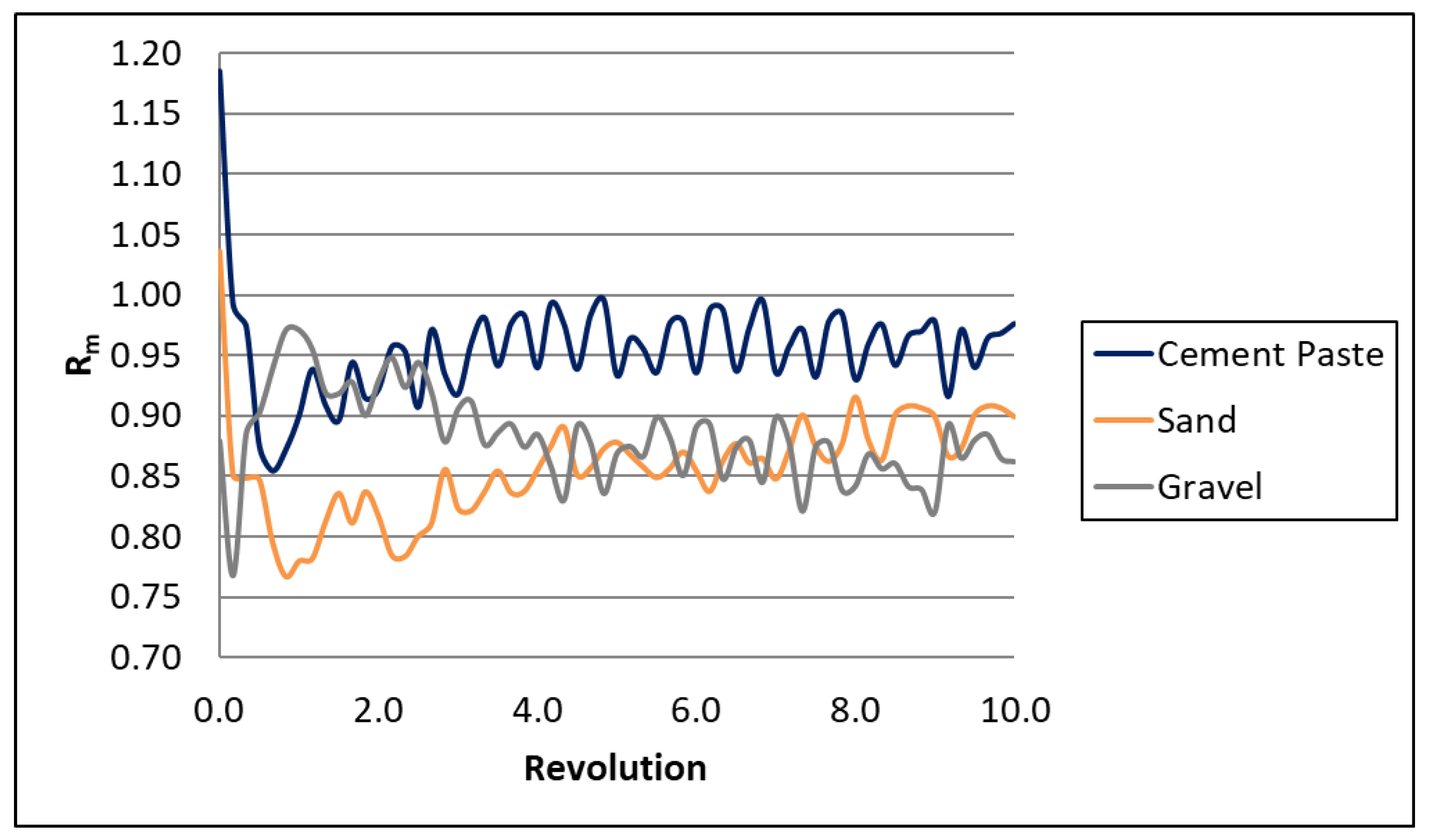
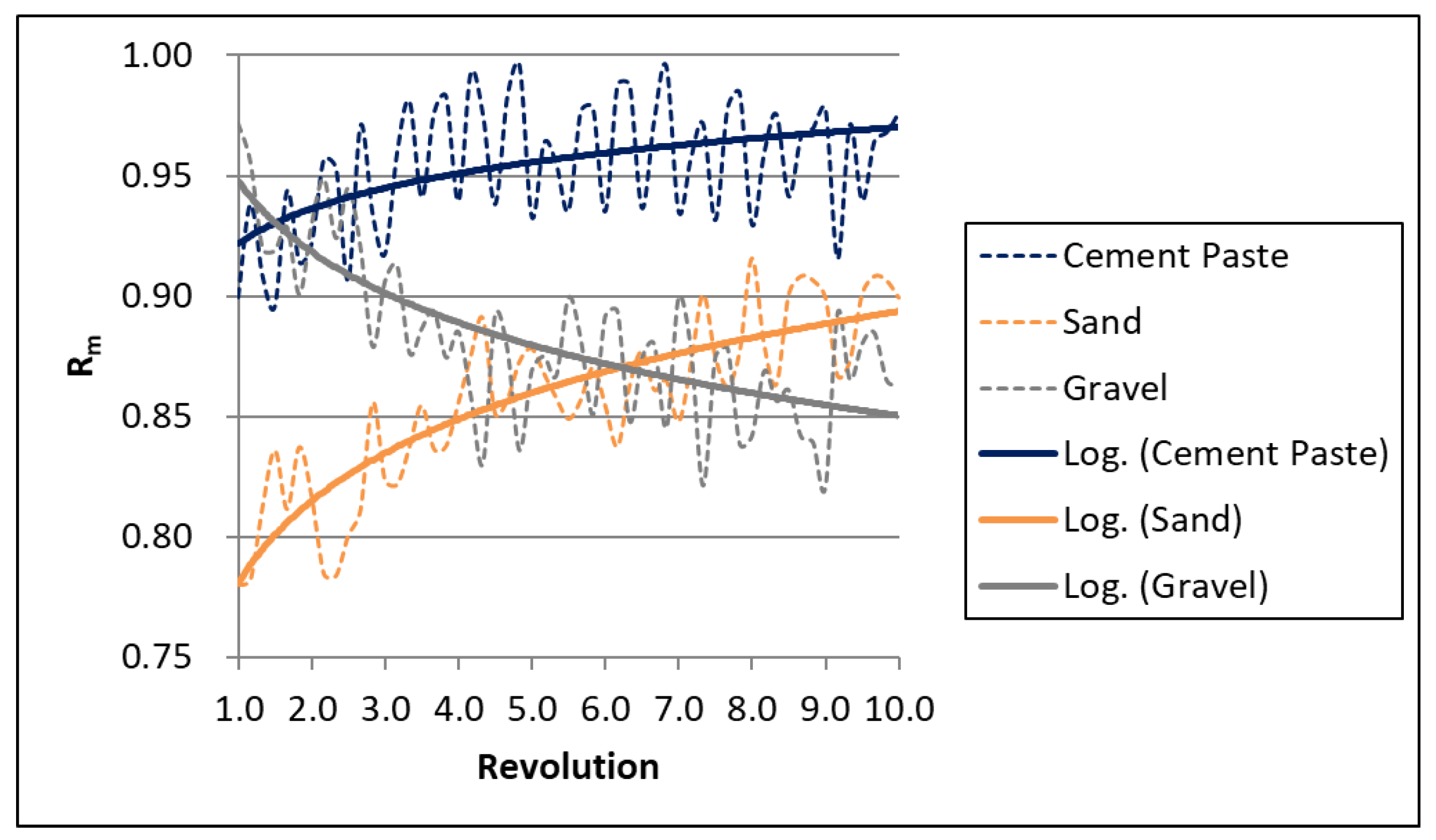
The curves referring to R_m tend to stabilize on a value less than unity. The reason is given by the presence of air in some points of the domain, which is absent in the mix design calculation thus reducing the effective volume fraction of the various phases in the considered elements.

-

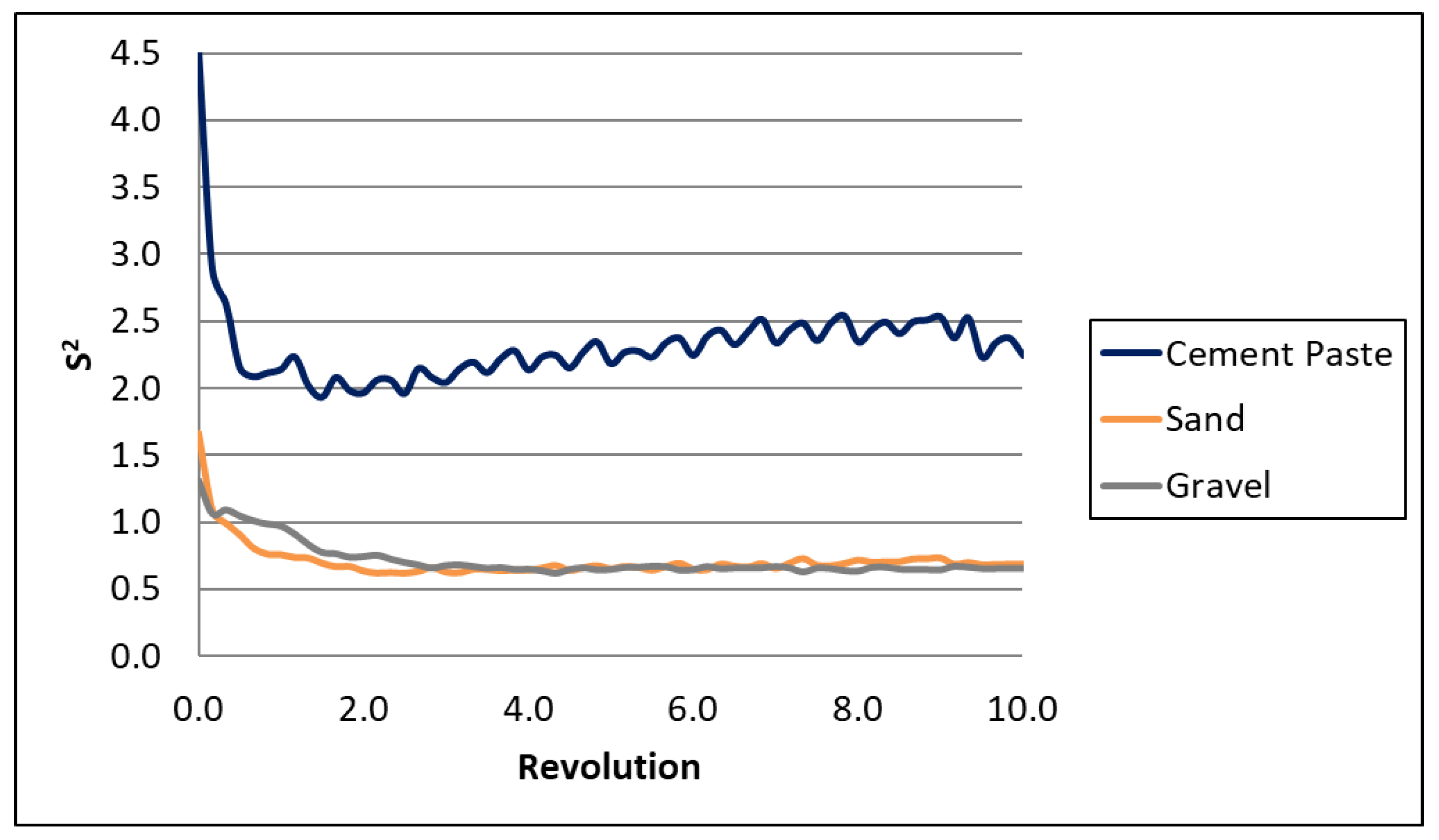
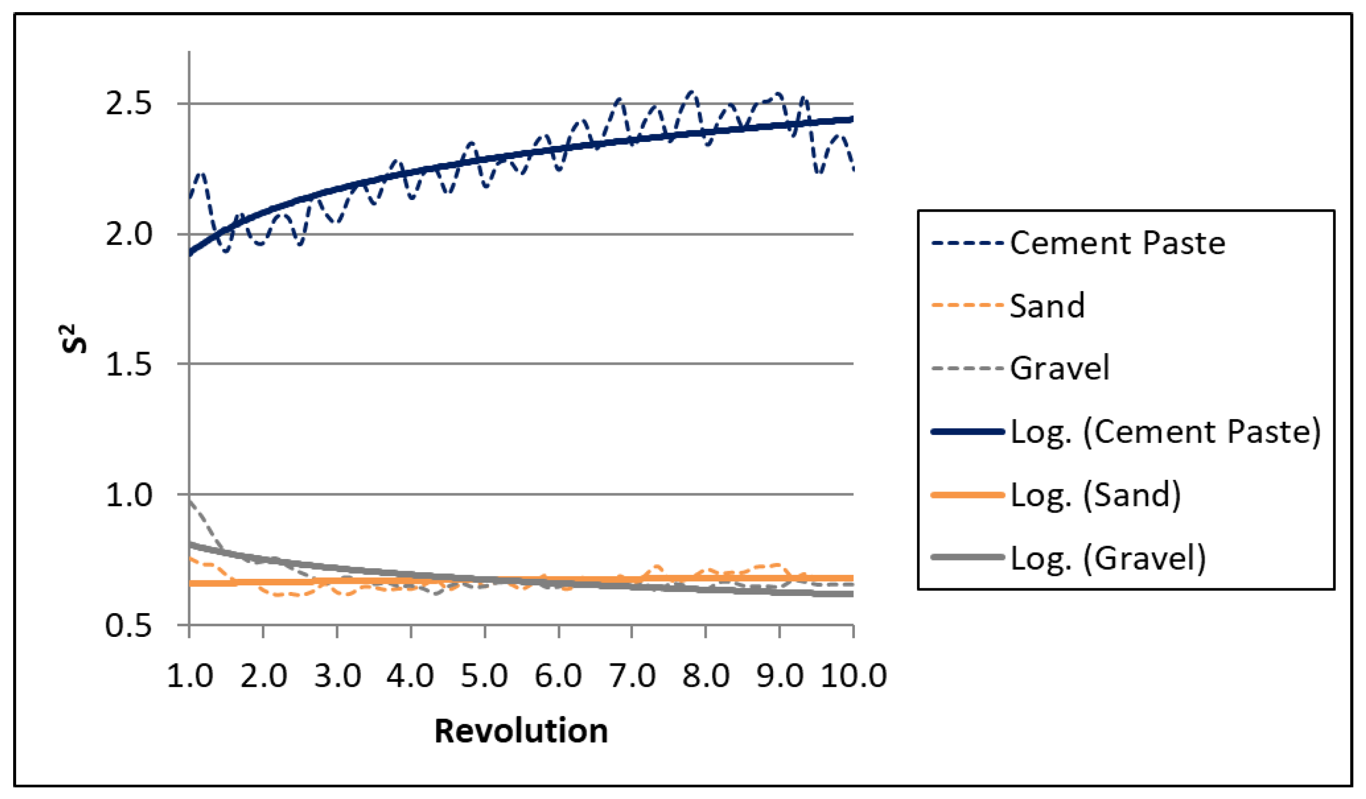
The S² curve of the cement paste stabilizes at much higher values than the solid phases, indicating less dispersion of the continuous phase within the analyzed domain.

The main problem resulting from this methodology pertains to the formulation of a correlation that provides a quality index of the distribution of the various phases within the geometry. In fact, for each simulation, there is a total of six time-varying parameters (R_m and S² for each individual phase of cement paste, sand, and gravel) that need to be compared in order to establish whether one geometry or dynamic parameter of the drum results in a better or worse distribution of the different phases than the others.

To do so, it was decided to take the values of the logarithmic trend curves associated with the trends as reference values for R_m and S² of each phase, calculated after 10 drum revolutions.

For certain simulations, it was decided to remove the numerical values given by the initial instants, as they were not indicative of the full convergence, so as to reduce the logarithmic trend error. The obtained logarithmic trend curves are shown in Figure 11 and Figure 12. From the logarithmic curves of S² and R_m, it is possible to obtain a distinct value at the considered revolution for each phase. At this point, it is possible, by means of the Gaussian distribution, to determine how the phases are distributed in the drum for each revolution. From the application of Equation (14), the curve shown in Figure 13 is obtained.

6. Conclusions and Future Perspectives

In a previous work [31], the authors developed a transient multiphase CFD model that simulated the distribution of aggregates in terms of gravel and sand of different grain sizes within cement paste in a concrete truck mixer. This work aimed to study the early stages of the concrete mixing process through an Eulerian CFD approach. Although the dispersion of various materials under the mechanical action of the drum blades was investigated, there was no quantitative method for calculating the mixing efficiency during drum rotation.

In this work, the statistical method for calculating the mixing index, defined as the ratio of the concentration of the considered phase (gravel, sand, or cement paste) in the i-th element to the optimal target concentration, was applied to the multiphase CFD model developed in the previous work. At the mixing index so defined, the terms of mean, variance, and probability density were calculated, which allowed the index to be extended from the cell (local) to the entire computational domain (concrete mixer). The establishment and implementation of the mixing index provided an effective means to evaluate the mixing process and its performance using a numerical Eulerian approach. This method ensured the precise assessment of mixing quality in the numerical study of mixers. Without the cell mixing index, such evaluations would be challenging, necessitating a shift to a Lagrangian approach. The cell mixing index was a crucial variable that enabled the analysis of multiphase mixing processes within the Eulerian numerical approach. By utilizing the model and applying the mixing index calculation as demonstrated in this study, it was possible to optimize the geometry and operational parameters, such as rotation speed and inclination.

The results showed that, after 10 revolutions, the gravel, sand, and cement paste reached the maximum distribution in the concrete truck mixer, equivalent to a steady-state value of the calculated mixing index. Furthermore, while the cement paste reached about 95% of the optimal distribution, the aggregates (sand and gravel), on the other hand, stopped between 85 and 90%. The values were intended to be averaged over the internal volume of the concrete mixer analyzed.

In conclusion, the following clarifications are presented:

The application of the mixing index as defined in this paper can only be applied if the target concentrations of the various species (mix design) are known.

-

The cell mixing index, as well as its extension to the whole computational domain by statistical functions, is a method not yet applied to the simulation of concrete mixing with an Eulerian–Eulerian approach.

-

The method can also be applied to other types of mixers.

-

The application of the mixing index to the CFD model makes it possible to predict the mixing efficiency of a mixer from the CAD of the geometry, so the method allows an optimized mixer design to be defined by reducing the number of prototypes.

-

The models for the simulation of concrete mixers are mainly CFD or DEM, in which the various phases are simulated through an Eulerian or Lagrangian approach, respectively. While for DEM-based models, the application of statistics to calculate the mixing index is sufficiently easy, precisely because they are based on the dynamics of an identifiable and well-defined number of particles, the application of the mixing index to the simulation of concrete mixing based on the Eulerian approach has not yet been defined and applied in this research area.

References

1. El-Emam, M.A.; Zhou, L.; Shi, W.; Han, C.; Bai, L.; Agarwal, R. Theories and Applications of CFD–DEM Coupling Approach for Granular Flow: A Review. Arch. Comput. Methods Eng. 2021, 28, 4979–5020. [Google Scholar] [CrossRef]
2. Hanley, K.J.; O’Sullivan, C.; Oliveira, J.C.; Cronin, K.; Byrne, E.P. Application of Taguchi methods to DEM calibration of bonded agglomerates. Powder Technol. 2011, 210, 230–240. [Google Scholar] [CrossRef]
3. Xu, J.; Wang, F.; Abegaz, R. State of the Art of CFD-DEM Coupled Modeling and Its Application in Turbulent Flow-Induced Soil Erosion. Geosciences 2025, 15, 21. [Google Scholar] [CrossRef]
4. Zhao, Z.; Zhou, L.; Bai, L.; Wang, B.; Agarwal, R. Recent Advances and Perspectives of CFD–DEM Simulation in Fluidized Bed. Arch. Comput. Methods Eng. 2024, 31, 871–918. [Google Scholar] [CrossRef]
5. Delmas, H.; Barthe, L.; Cleary, R. Chapter 29—Ultrasonic mixing, homogenization, and emulsification in food processing and other applications. In Power Ultrasonics, 2nd ed.; Woodhead Publishing Series in Electronic and Optical Materials; Woodhead Publishing: Cambridge, UK, 2023; pp. 665–685. ISBN 9780128202548. [Google Scholar] [CrossRef]
6. Gall, V.; Runde, M.; Schuchmann, H.P. Extending Applications of High-Pressure Homogenization by Using Simultaneous Emulsification and Mixing (SEM)—An Overview. Processes 2016, 4, 46. [Google Scholar] [CrossRef]
7. Hlosta, J.; Jezerská, L.; Rozbroj, J.; Žurovec, D.; Nečas, J.; Zegzulka, J. DEM Investigation of the Influence of Particulate Properties and Operating Conditions on the Mixing Process in Rotary Drums: Part 2—Process Validation and Experimental Study. Processes 2020, 8, 184. [Google Scholar] [CrossRef]
8. Jadidi, B.; Ebrahimi, M.; Ein-Mozaffari, F.; Lohi, A. A comprehensive review of the application of DEM in the investigation of batch solid mixers. Rev. Chem. Eng. 2023, 39, 729–764. [Google Scholar] [CrossRef]
9. Chen, Y.; Chang, X.; Zhang, B.; Huang, H. Efficient and effective calibration of numerical model outputs using hierarchical dynamic models. Ann. Appl. Stat. 2024, 18, 1064–1089. [Google Scholar] [CrossRef]
10. Coetzee, C.J. Review: Calibration of the discrete element method. Powder Technol. 2017, 310, 104–142. [Google Scholar] [CrossRef]
11. Hesse, R.; Krull, F.; Antonyuk, S. Experimentally calibrated CFD-DEM study of air impairment during powder discharge for varying hopper configurations. Powder Technol. 2020, 372, 404–419. [Google Scholar] [CrossRef]
12. Magri, L.; Sequino, L.; Ferrari, C. Simulating the Electrochemical-Thermal Behavior of a Prismatic Lithium-Ion Battery on the Market under Various Discharge Cycles. Batteries 2023, 9, 397. [Google Scholar] [CrossRef]
13. Wasserfall, J.G.; Coetzee, C.J.; Meyer, C.J. A submerged draw down test calibration method for fully-coupled CFD-DEM modelling. Front. Chem. Eng. 2024, 6, 1376974. [Google Scholar] [CrossRef]
14. Hema, V.; Savithri, S. Mathematical Modelling of the Dynamics of Granular Materials in a Rotating Cylinder. Ph.D. Thesis, Cochin University of Science and Technology, Kochi, India, 2003. Available online: http://ir.niist.res.in:8080/jspui/handle/123456789/1173 (accessed on 21 August 2024).
15. Panneerselvam, R.; Savithri, S.; Surender, G.D. CFD modeling of gas– liquid–solid mechanically agitated. Chem. Eng. Res. Des. 2008, 86, 1331–1344. [Google Scholar] [CrossRef]
16. Poux, M.; Fayolle, P.; Bertrand, J.; Bridoux, D.; Bousquet, J. Powder mixing: Some practical rules applied to agitated systems. Powder Technol. 1991, 86, 213–234. [Google Scholar] [CrossRef]
17. Rhodes, M.J.; Wang, X.S.; Nguyen, M.; Stewart, P.; Liffman, K. Study of mixing in gas-fluidized beds using a DEM model. Chem. Eng. Sci. 2001, 56, 2859–2866. [Google Scholar] [CrossRef]
18. Lacey, P.M.C. Developments in the theory of particle mixing. J. Appl. Chem. 1954, 4, 257–268. [Google Scholar] [CrossRef]
19. Harnby, N.; Edwards, M.F.; Nienow, A. Mixing in the Process Industries; Butterworth-Hinemann: Oxford, UK, 1997. [Google Scholar]
20. Khopkar, A.R.; Kasat, G.R.; Pandit, A.B.; Ranade, V.V. CFD simulation of mixing in tall gas–liquid stirred vessel: Role of local flow patterns. Chem. Eng. Sci. 2006, 61, 2921–2929. [Google Scholar] [CrossRef]
21. Khopkar, A.R.; Kasat, G.R.; Pandit, A.B.; Ranade, V.V. Computational fluid dynamics simulation of the solid suspension in a stirred slurry reactor. Ind. Eng. Chem. Res. 2006, 45, 4416–4428. [Google Scholar] [CrossRef]
22. Murthy, B.N.; Ghadge, R.S.; Joshi, J.B. CFD simulations of gas–liquid–solid stirred reactor: Prediction of critical impeller speed for solid suspension. Chem. Eng. Sci. 2007, 62, 7184–7195. [Google Scholar] [CrossRef]
23. Till, Z.; Molnàr, B.; Egedy, A.; Varga, T. CFD Based Qualification of Mixing Efficiency of Stirred Vessels. Period. Polytech. Chem. Eng. 2019, 63, 226–238. [Google Scholar] [CrossRef]
24. Ameur, H. Energy efficiency of different impellers in stirred tank reactors. Energy 2015, 93, 1980–1988. [Google Scholar] [CrossRef]
25. Park, C.; Lee, K.; Hong, S.; Lee, J.; Cho, S.; Moon, I. Novel index for evaluating continuous mixing process with pulse injection of bimodal tracer particles. Powder Technol. 2019, 355, 309–319. [Google Scholar] [CrossRef]
26. Wallewik, J.E.; Wallewik, O.H. Analysis of shear rate inside a concrete truck mixer. Cem. Concr. Res. 2017, 95, 9–17. [Google Scholar] [CrossRef]
27. Stepanov, V.; Kireev, S. Efficiency Analysis for Mechanical Mixing Systems of Cementing Units. In Networked Control Systems for Connected and Automated Vehicles. NN 2022; Guda, A., Ed.; Lecture Notes in Networks and Systems; Springer: Cham, Switzerland, 2023; Volume 510. [Google Scholar] [CrossRef]
28. Li, S.P.; Yuan, Y.L.; Shi, L.G. Research on CFD Simulation of the Cement Slurry Mixer. Adv. Mater. Res. 2012, 621, 196–199. [Google Scholar] [CrossRef]
29. Beccati, N.; Ferrari, C.; Bonanno, A.; Balestra, M. Calibration of a CFD discharge process model of an off-road self-loading concrete mixer. J. Braz. Soc. Mech. Sci. Eng. 2019, 41, 76. [Google Scholar] [CrossRef]
30. Beccati, N.; Ferrari, C. Predicting the capacity of an off-road self-loading drum mixer with different concrete consistencies through three-dimensional fluid dynamics analysis. J. Braz. Soc. Mech. Sci. Eng. 2020, 42, 379. [Google Scholar] [CrossRef]
31. Ferrari, C.; Beccati, N. Mixing Phase Study of a Concrete Truck Mixer via CFD Multiphase Approach. J. Eng. Mech. 2022, 148, 04022002. [Google Scholar] [CrossRef]
32. Ansys. CFX-Solver Theory Guide R19.2; Ansys: Canonsburg, PA, USA, 2019. [Google Scholar]
33. Ansys. Ansys Icem CFD User Manual; Ansys: Canonsburg, PA, USA, 2019. [Google Scholar]
34. Wierig, H.J. Properties of Fresh Concrete; Chapman and Hall: New York, NY, USA, 1990. [Google Scholar]
35. Sahin, Y.; Akkaya, Y.; Boylu, F.; Tasdemir, M.A. Characterization of air entraining admixtures in concrete using surface tension measurements. Cem. Concr. Compos. 2017, 82, 95–104. [Google Scholar] [CrossRef]
36. Brackbill, J.U.; Kothe, D.B.; Zemach, C.A. Continuum Method for Modeling Surface Tension. J. Comput. Phys. 1992, 100, 335–354. [Google Scholar] [CrossRef]
37. Paul, E.L.; Atiemo-Obeng, V.A.; Kresta, S.M. Handbook of Industrial Mixing: Science and Practice; Wiley: New York, NY, USA, 2004. [Google Scholar]
38. Crowe, C.T.; Sommerfield, M.; Tsuj, Y. Multiphase Flows with Droplets and Particles; CRC Press: Boca Raton, FL, USA, 1998. [Google Scholar] [CrossRef]
Figure 1. Drum geometry.
Fluids 10 00072 g001
Figure 2. Examples of block layers with O-grids applied to the drum.
Fluids 10 00072 g002
Figure 3. Experimental test of discharge process with sand.
Fluids 10 00072 g003
Figure 4. Comparison of the numerical testing discharge curves [31].
Fluids 10 00072 g004
Figure 5. Dimensionless torque curve of the truck drum measured during the mixing phase (green), comparison with simulated curve (yellow), 20% error bar.
Fluids 10 00072 g005
Figure 6. Variance as a function of the number of grid elements.
Fluids 10 00072 g006
Figure 7. Surface streamlines of the flow.
Fluids 10 00072 g007
Figure 8. Volume fraction contour plots at different revolutions of the drum.
Fluids 10 00072 g008
Figure 9. Rm of cement paste, sand, and gravel as the drum revolutions increase.
Fluids 10 00072 g009
Figure 10. S2 of cement paste, sand, and gravel as the drum revolutions increase.
Fluids 10 00072 g010
Figure 11. Rm logarithmic trend for cement paste, sand, and gravel.
Fluids 10 00072 g011
Figure 12. S2 logarithmic trend for cement past, sand, and gravel.
Fluids 10 00072 g012
Figure 13. Probability density of the mixing index.
Fluids 10 00072 g013