Abstract
This paper simulates the blood clot extraction process inside an idealized cylindrical blood vessel model using the aspiration-based thrombectomy technique. A fully Eulerian technique is used within the finite volume method where incompressible Navier–Stokes equations are solved in the fluid region. In contrast, the Cauchy stress equation is solved in the clot region. Blood is assumed to be a Newtonian fluid, while the clot is either hyperelastic or viscoelastic material. In the hyperelastic formulation, the clot deformation is calculated based on the left Cauchy–Green deformation tensor, while the stresses are based on the linear Mooney–Rivlin model. In the viscoelastic formulation, the Oldroyd B model is used within the log conformation approach to calculate the viscoelastic stresses in the clot. The interface between the blood and the clot is tracked with the help of the geometric volume-of-fluid method. We focus on the role of flow variables like the pressure, velocity, and proximity between the clot and the catheter tip to successfully capture the clot under catheter suction. We observe that, once the clot is attracted to the catheter port due to pressure forces, the viscous stresses try to drag it inside the catheter. On the other hand, if the clot is not initially attracted, it is carried downstream by the viscous stresses. If the suction velocity is low (∼0.2 m/s), the clot cannot be sucked inside the catheter, even if it is touching the catheter. At a higher suction velocity of 0.4 m/s, the suction effect is strong enough to capture the clot despite the larger initial distance from the catheter. Hence, the pressure distribution and viscous stresses play essential roles in the suction or escape of the clot during the thrombectomy process. Also, the viscoelastic model predicts the rupture of the clot inside the catheter during suction.
1. Introduction
Ischemic strokes cause a significant number of the annual deaths worldwide [1]. Moreover, the frequency of ischemic stroke has recently increased following the outbreak of COVID-19 [2]. A stroke occurs when a blood clot forms inside cerebral vessels due to an injury and blocks the blood supply that carries oxygen to the cells and tissues downstream of the occlusion site. The clot can also form inside the major blood vessels supplying blood to the brain, and it may break/detach, drift, and finally occlude the finer vessels inside the brain. The clinical remedy in a stroke situation is to remove the clot from the occluded site and restart the blood supply as quickly as possible. Otherwise, the oxygen-deprived cells and tissues start dying without oxygen. Suction-based mechanical aspiration is one of the available techniques, under which a clot is sucked and extracted with the help of a catheter [3,4,5,6,7]. The primary variables that control the outcome of this technique are the suction velocity/pressure and the distance between the clot and the catheter tip. A smaller suction pressure does not produce sufficient suction force to pull the clot, while too large a suction pressure can deprive the blood supply for branching capillaries upstream of the occlusion site. An excessive suction force may even cause the collapse of the blood vessel itself, or it can cause damage to the vessel wall, creating more clot formation sites [8]. Additionally, there is uncertainty concerning the minimum required distance between the catheter tip and the thrombus. For successful extraction, Lally et al. [9] observed that direct contact is required between the catheter tip and the thrombus. Keeping the above discussion in mind, a systematic study is needed to quantify the effect of the parameters that govern the aspiration process and provide further insights into the dynamics of the thrombectomy process. This provided us with the motivation for the current study, in which we use simulations to investigate the thrombectomy dynamics.
The simulation of motion and the deformation of solids submerged in flowing fluids involves complexities in any fluid–structure interaction numerical analysis. Traditionally, either the segregated or the fully coupled approach is used for such simulations. In the segregated approach, the fluid flow and the solid deformation problems are solved separately on solvers dedicated to these problems, with the force and deformation-related data transfers at the interface being facilitated by third-party libraries (see, for example, PreCICE [10]). The fully coupled approach deals with the problem using Arbitrary Lagrangian–Eulerian (ALE)-based formulations [11]. Both these formulations suffer under extreme deformations of the solid, which requires frequent remeshing of the computational domain. Alternative formulations have been proposed to tackle the problem of mesh movement or remeshing. One such approach is based on the immersed boundary method, where the flow is solved on a background Eulerian mesh while the deformation and motion of the solid are solved in a Lagrangian manner [12,13]. The forces from the discrete locations on the solid are transferred to the Eulerian mesh using smoothed Dirac delta functions. The solid domain may still require remeshing under extreme deformations in this approach. Yet another formulation is the fully Eulerian approach, where the fluid flow, solid motion, and deformation are solved in a Eulerian manner. The interface between the fluid and solid is tracked with interface tracking/capturing approaches like the volume-of-fluid, level-set, or phase field methods. The fluid flow solution does not challenge the Eulerian grid, but the solid deformation/motion requires the Eulerian form of the material constitutive equations. Additionally, the formulation faces convergence issues when stiff solids are involved. The numerical diffusion and dispersion present inherently in Eulerian grid-based formulations smooth out any sharp corners present on the solid. This can be controlled to some extent using local mesh refinement and higher-order schemes. The technique provides simplicity in implementation and has been successfully used to simulate the motion of soft solids immersed in fluids.
In the following, we briefly summarize the previous works on the Eulerian formulation of flows with immersed solids. Some researchers in the literature directly evolved the left Cauchy–Green deformation tensor components, which are used to calculate the deformation and stresses in the immersed solid. Zhao et al. [14] proposed a finite-difference-method-based Eulerian formulation to simulate soft biological materials immersed in fluids. The stresses in the solid were calculated using a Lagrangian mesh with the finite element method. The forces from inside the solid were modeled as body forces in the fluid solver, while the surface forces from the fluid–solid interface were transferred to the Eulerian mesh using immersed boundary methods. Two-dimensional problems like flow inside a cavity with a deformable wall, motion of a flexible leaflet inside a channel, oscillation and motion of a deformable disk in a cavity, motion of a jellyfish-like structure, etc., have been investigated. Sugiyama et al. [15] studied the motion and interaction of bi-concave discoid particles (mimicking red blood cells) made up of a neo-Hookean material inside a two-dimensional Poiseuille flow. The authors used the fifth-order WENO scheme [16] for the advection terms in the governing equations and the second-order Adam–Bashforth or Crank–Nicolson schemes for the temporal derivatives. They applied the finite difference method to discretize the governing equations on a Eulerian grid. They solved the first-order advection equation for the evolution of the fluid–solid boundary. They used the formulation based on the left Cauchy–Green deformation tensor to calculate the solid particles’ stresses. Sugiyama et al. [17] proposed a finite difference method based on a full Eulerian scheme for the fluid–structure interaction problems. The authors used the volume-of-fluid method to track the interface between the fluid and the solid phases. They updated the left Cauchy–Green tensor components for the solid deformation under neo-Hookean, Mooney–Rivlin, and Saint Venant–Kirchhoff material laws. The authors investigated problems like the motion of a two-dimensional oscillating solid rod sandwiched between viscous fluid layers inside a channel, the motion of a circular deformable disk inside a driven cavity, and the motion of circular and rectangular solids inside a channel, etc. Ii et al. [18] implemented an implicit version of the formulation presented by Sugiyama et al. [15] for the simulation of stiff/hard solids immersed in fluid flows. The numerical instability and the short time step restriction with stiff solids (which plagued the original version) were avoided with the implicit formulation. Ii et al. [19] investigated the motion of multiple red blood cells and platelets inside a capillary vessel. Their numerical formulation took into account an extra membrane force based on the evolution of the surface component of the left Cauchy–Green deformation tensor. The authors investigated the shear-induced motion of deformable particles inside a channel. Using the artificial compressibility method for the Navier–Stokes equation, Sugiyama et al. [20] used their earlier formulation to study the motion of many red blood cells and platelets inside a three-dimensional micro-channel. Farahbakhsh et al. [21] took a slightly different approach to solve the fluid flow problem. They used a vorticity–stream-function-based approach for solving the Navier–Stokes equations in two dimensions. The deformation in the solid was based on an evolution equation for the left Cauchy–Green tensor, and stresses were calculated using the Mooney–Rivlin and Saint Venant–Kirchhoff hyperelastic models. They studied two-dimensional flow inside a cavity with a deformable wall, oscillation of a circular elastic disk, and the motion of bi-concave deformable particles. Using the vorticity–stream function approach along with the immersed boundary method, Faranbaksh et al. [22] simulated the motion of an elastic ring and multiple deformable bi-concave solids inside a channel with rigid obstacles. Earlier, this group used the same approach for studying the motion of rigid solids inside a fluid [21,23].
Here, we summarize the previous works on clot extraction using thrombectomy techniques. Using three-dimensional computational-fluid-dynamics-based calculations, Shi et al. [24] determined the variation of suction force acting on a plugged blood vessel end with respect to the distance from a catheter tip. They observed a suction force of around 0.07 N when the catheter almost touched the plug. The force decreased by a factor of 10 within a distance of 1 mm, beyond which the force remained almost constant. Tashiro et al. [25] conducted experiments and numerical simulations on the mechanical response of blood clots under cyclic loading and unloading conditions. They observed that the Mooney–Rivlin model described the clot hyperelasticity while the three-chain Oldroyd B model accurately described viscoelasticity. They also observed that the fibrinogen-dosed clot was three times stiffer than the pure blood clot. Assuming viscoelastic solid behavior based on the Kelvin Voigt model, Oyekole et al. [26] studied the cyclic-aspiration-based recanalization procedure for ischemic stroke. They included a viscoelastic cohesive zone between the hyperelastic artery wall and the viscoelastic clot. They observed that the clot surface first separates from the artery wall at the distal end, and then the failure propagates towards the proximal end. Using a hyperelastic artery model and a nonlinear viscoelastic clot model along with a cohesive zone between the clot surface and the artery wall, Patki et al. [8] analyzed the effect of clot length on the recanalization process under cyclic aspiration conditions. During the aspiration process, they observed clots with length-to-radius ratios greater than two separate from the arterial inner surface. They also studied the possibility of artery wall endothelial cell damage near the suction tip of the catheter. Using an Arbitrary Lagrangian–Eulerian technique, Mirakhorli et al. [27] investigated the motion of a clot inside a branch of pulmonary arteries. They observed higher clot velocity with a visco-hyperelastic clot model than the hyperelastic model. They also observed that the clot could sustain stresses of the order of 165 Pa throughout 0.01 s. Luisi et al. [28] developed experimental and simulation-based techniques for investigating cerebral artery flow and pressure redistribution during aspiration thrombectomy. They concluded that changes in the flow distribution depend on the occlusion severity and the volume flow rate of the blood extracted by the catheter.
Based on the above discussion, we conclude that the fully Eulerian-based formulations are reliable for simulating fluid–soft solid interaction problems. Compared to other fluid–structure interaction-based approaches, the techniques are simple to implement and computationally efficient. In this work, we perform a direct numerical simulation of the clot extraction process using a fully Eulerian formulation. Based on the finite volume method, the formulation is implemented in the open-source flow solver Basilisk [29]. We assume blood is a Newtonian fluid, while the clot is considered a hyperelastic or viscoelastic material. Under the hyperelastic model, the nonlinear Mooney–Rivlin material model is used for calculating the stresses. The model details can be found in [30]. The solid deformation and stresses are solved using direct evolution of the left Cauchy–Green tensor components and the Mooney–Rivlin model. The Oldroyd B model is used within the log conformation approach for calculating the viscoelastic stresses. The interface between the blood and the clot is captured with the help of the geometric volume of fluid, which is conservative and non-diffusive [31]. The problem at hand is a challenging one that involves the simultaneous solution of fluid flow and clot deformation and tracking of the interfaces between these materials, the constitutive behavior of the clot material with finite deformation, and the presence of rigid obstacles (catheter material), etc. Thanks to the creators of Basilisk, the problem can be efficiently tackled using open-source software. This manuscript is organized as follows: in Section 2, we present the governing equations and the details of the numerical implementation; in Section 3, we discuss the computational domain and the boundary conditions; in Section 4, we present and discuss the various results obtained by the numerical simulations; finally, in Section 5, we conclude the current work.
2. Governing Equations, Numerical Algorithm, and Validation
Basilisk solves the following equations with the finite volume method. The equations govern the conservation of mass and momentum for incompressible, isothermal flows.
Equation (1), the continuity equation, says that the velocity field must be divergence free for incompressible flows. Equation (2) implies that the momentum of the fluid in an infinitesimal control volume changes due to several factors like the imbalance in the rate at which momentum crosses the faces of the control volume, pressure gradient, divergence of viscous, hyperelastic, and viscoelastic stresses, etc.
In the above equations, denotes density, denotes viscosity, and denote the density and dynamic viscosity of the blood, respectively, and are the density and dynamic viscosity of the clot, respectively, p denotes pressure, denotes the velocity vector, is the rate of the deformation tensor, are the elastic stresses in the clot, and, finally, are the viscoelastic stresses in the clot. We neglect surface tension and gravity forces in the current work, although they are already implemented in Basilisk. The interface between the blood and the clot is tracked with the help of the following advection equation written in terms of clot fraction :
The evolution equation for the left Cauchy–Green deformation tensor is
This tensor is defined in the spatial or deformed configuration and is used to describe the deformation of the blood clot. The Cauchy stresses inside a material are given by
For the linear Mooney–Rivlin material, is assumed to be zero [30], while, for a neo-Hookean material, both and are zero and where G is the shear modulus.
For viscoelastic flows, the divergence of polymeric stresses is added to the Navier–Stokes equation, Equation (2), in place of the divergence of hyperelastic stresses . The governing equation for the polymeric stresses is given by
Directly solving the above equations is prone to a numerical instability called High Weissenberg number instability. Instead, the following equation, for the conformation tensor , is considered:
The polymeric stresses and the conformation tensor are related by . For numerical-robustness-related reasons, the following equation for the log conformation tensor is actually solved:
In the above equation, and are tensors resulting from the following decomposition: . Further details on the viscoelastic formulation can be found in [32,33].
Basilisk uses a second-order, accurate, staggered-in-time discretization approach in which the governing equations are as follows:
The above equations are solved using a time-split projection method.
The viscous terms in the Navier–Stokes equations are treated implicitly in the above equations. This way, larger time steps can be used while maintaining a stable calculation procedure. The convection term is discretized using an unsplit Bell–Collela–Glaz scheme. At the same time, the pressure velocity coupling is solved using a projection method, resulting in an overall second-order accurate Navier–Stokes formulation [34]. Further details on the algorithm can be found in [35,36]. Left Cauchy–Green deformation tensor components evolve in time using an implicit formulation that requires the solution of Poisson–Helmholtz equations. These equations are solved with the help of a multigrid-based solver. The hyperelastic stresses in the clot are then solved using Equation (5) in the following form:
where the coefficients are given by , , , and, finally, . This formulation for the components of the left Cauchy–Green deformation tensor and hyperelastic stresses was provided by Lopez [37].
To validate the solver, Figure 1 shows the results on the motion of a two-dimensional circular soft solid inside a driven cavity. The reference results are from Zhao et al. [14]. The problem was also studied on a 1024 × 1024 grid by Sugiyama et al. [17], and the same problem was also discussed by Jain et al. [38]. The results in the colored outline are based on the current simulations. As can be seen in the figure, the shape of the solid is captured well in our simulations, also on a 512 × 512 grid. Based on this, we conclude that the current formulation is accurate enough to capture the dynamics of soft solids submerged in viscous fluids.
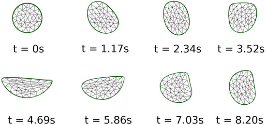
Figure 1.
Comparison of the current numerical results on the motion of a two-dimensional soft solid inside a driven cavity with those in previous literature. The current results in the green-colored outline are on a grid of 512 × 512, while those shown with a triangular mesh are from Zhao et al. [14].
3. Computational Domain and Boundary Conditions
The computational domain is shown in Figure 2. The length of the domain used in the current work is mm, the diameter of the idealized blood vessel is mm, the diameter of the catheter is mm, the thickness of the catheter wall is mm, the length of the suction tube or the catheter is mm, the clot diameter is mm, and, finally, two different values are taken for the clot distance from the catheter tip . A suction velocity of either 0.2 m/s or 0.4 m/s is applied to the catheter’s suction port at the domain’s right boundary. A fixed velocity of −0.6 m/s is used at the inlet of the artery model (outside the suction port) at the right boundary. These are the typical values of the suction velocity and the flow velocity inside the middle cerebral artery in the human brain. A fixed pressure value equal to 0 Pa and the homogeneous Neumann condition for the velocity are applied to the left boundary of the domain. It should be noted here that the absolute magnitude of the pressure is not essential for incompressible flows. Rather, the pressure gradient is necessary. The no-slip condition is applied to the walls of the model. Such a model representation excludes important real-vessel characteristics such as curvature, branching, and compliance, but simplification is necessary due to numerical feasibility. The simulations are carried out on a locally refined grid where the grid is at the finest level of 10 around the interface between the blood and the clot and the coarsest grid level is 9. A grid level of 9 implies a minimum of grid cells along the length of the computational domain. The grid is locally and dynamically refined to level 10 as the blood–clot interface moves in the domain. Various physical properties of the blood and the clot used in the current work are shown in Table 1.
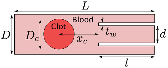
Figure 2.
Computational domain for the clot extraction problem. In this work, the length of the blood vessel is mm, the diameter of the blood vessel is mm, the diameter of the catheter is mm, the thickness of the catheter wall is mm, the length of the catheter is mm, the diameter of the clot is mm, and, finally, two different values are investigated for the clot distance from the catheter tip .

Table 1.
Various physical properties of the fluid and solid used in the simulations.
We further perform a grid independence study, and the results are shown in Figure 3. The figure shows the interface profiles after every millisecond on two different grids. The red–blue contours are on the level 10 grid ( grid cells along the length of the domain), while the black outline is the interface boundary on the level 11 grid ( grid cells along the length of the domain). As can be noticed in the figure, there is a minor difference in the shape of the blood–clot interface on the two grids, based on which we conclude that the level 10 grid is sufficient for capturing the clot dynamics during suction. In the next section, we present and discuss the results of the current simulations.
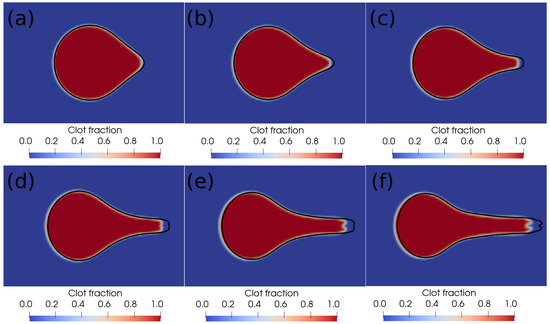
Figure 3.
Interface profiles at different times on two different grids. (a) Time ms, (b) time ms, (c) time ms, (d) time ms, (e) time ms, (f) time ms. The red–blue contours are on the level 10 grid ( grid cells along the length of the domain), and the black outline is the interface boundary on the level 11 grid ( grid cells along the length of the domain).
4. Results and Discussion
Here, we discuss the different results related to clot aspiration. First, we discuss the results based on the hyperelastic formulation, and, later, we present the results based on the viscoelastic formulation.
4.1. Results Based on Hyperelastic Formulation
In this subsection, first, we present the results on clot escape at a lower suction velocity of 0.2 m/s, and, later, we present the clot suction cases at a higher suction velocity of 0.4 m/s. For visualization purposes, we show the clot–blood interface shapes filled with the contours of different stress components.
4.1.1. Clot Escape Cases at Lower Suction Velocity of 0.2 m/s
In this subsection, we present the cases of failed suction of a clot due to a lower suction velocity of 0.2 m/s. If the clot is initially far from the catheter, as in Figure 4, and the suction velocity is small, ∼0.2 m/s, the clot is carried away from the catheter tip by the flowing stream of blood. The clot does not feel the suction effect at a larger distance from the catheter tip. Figure 4 further shows the standard and shear components of the elastic stresses developed in the clot due to its deformation.
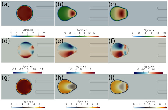
Figure 4.
Elastic stress components (in Pascal) inside the clot at different times. (a) at 1 ms, (b) at 10 ms, (c) at 20 ms, (d) at 1 ms, (e) at 10 ms, (f) at 20 ms, (g) at 1 ms, (h) at 10 ms, (i) at 20 ms. The initial distance between the clot and the catheter is 1.05 times the clot radius. Suction velocity is 0.2 m/s, blood flow velocity is −0.6 m/s. = 0.58, = 0.78, = 0. The suction effect is not strong enough to pull the clot.
If the clot is almost touching the catheter tip, pressure forces under the suction effect try to pull the clot, as shown in Figure 5, but the viscous forces on the periphery of the clot overwhelm the suction effect, and the clot again escapes the catheter. We observe that, if the suction velocity is low (∼0.2 m/s), the clot cannot be sucked inside the catheter even if it is touching the catheter. The primary reason is that the viscous forces on the clot surface exerted by the incoming bloodstream are stronger than the suction force created by the pressure difference.
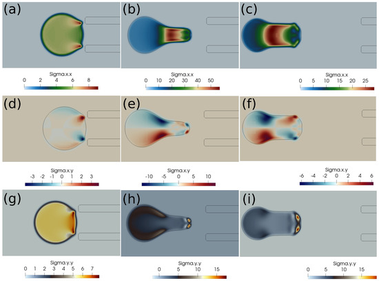
Figure 5.
Elastic stress components (in Pascal) inside the clot at different times. (a) at 1 ms, (b) at 10 ms, (c) at 20 ms, (d) at 1 ms, (e) at 10 ms, (f) at 20 ms, (g) at 1 ms, (h) at 10 ms, (i) at 20 ms. The initial distance between the clot and the catheter is 0.75 times the clot radius. Suction velocity is 0.2 m/s, flow velocity is −0.6 m/s. = 0.58, = 0.78, = 0. The suction effect tries to pull the clot but is unsuccessful in capturing it.
4.1.2. Clot Capture Cases at Higher Suction Velocity of 0.4 m/s
Here, we discuss the clot capture cases under a higher suction velocity of 0.4 m/s. Figure 6 shows the clot interface filled with the contours of normal stress . At a higher suction velocity of 0.4 m/s, the suction effect is strong enough to capture the clot despite the larger initial distance of the clot from the catheter. With a higher aspiration velocity, a portion of the clot is sucked initially due to pressure difference, which reduces the surface area of the unsucked portion of the clot. Therefore, the surface viscous forces due to the incoming bloodstream (outside the catheter) keep on decreasing while the clot is sucked inside the catheter. The outcome is the clot’s suction despite the larger initial separation of the clot from the catheter tip.
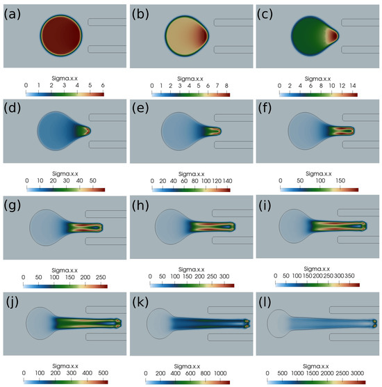
Figure 6.
Normal stress component (Pascal) inside the clot at different times. (a) Time ms, (b) time ms, (c) time ms, (d) time ms, (e) time ms, (f) time ms, (g) time ms, (h) time ms, (i) time ms, (j) time ms, (k) time ms, (l) time ms. The initial distance between the clot and the catheter is 1.05 times the clot radius. Suction velocity is 0.4 m/s, flow velocity is −0.6 m/s. = 0.58, = 0.78, = 0. The suction effect is strong enough to capture the clot in spite of the larger initial distance from the catheter.
4.1.3. Role of Pressure and Viscous Stresses in Pulling the Clot
In this subsection, we investigate the clot suction and escape mechanisms further. In particular, we focus on the role of pressure during the suction of the clot. Figure 7 shows the pressure distribution, while Figure 8 shows the velocity vector distribution for the clot suction case at a higher suction velocity of 0.4 m/s. It may be noticed from Figure 7 that a pressure difference of 100 Pa always acts across the clot interface as the catheter sucks it. Once the clot is sucked, the high velocity between the clot and the catheter wall exerts high shear forces over the clot surface, as can be seen from the velocity distribution in Figure 8. These viscous stresses drag the clot inside the catheter and help suction of the clot.
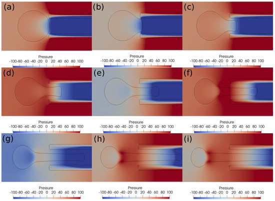
Figure 7.
Pressure contours around the clot at different times. (a) Time ms, (b) time ms, (c) time ms, (d) time ms, (e) time ms, (f) time ms, (g) time ms, (h) time ms, (i) time ms. The initial distance between the clot and the catheter is 0.75 times the clot radius. Suction velocity is 0.4 m/s, flow velocity is −0.6 m/s. = 0.58, = 0.78, = 0. A pressure difference of around 100 Pa always acts across the clot in spite of its suction inside the catheter.
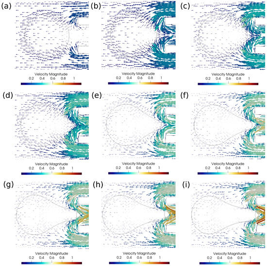
Figure 8.
Velocity vectors around the clot for the successful clot suction case. (a) Time ms, (b) time ms, (c) time ms, (d) time ms, (e) time ms, (f) time ms, (g) time ms, (h) time ms, (i) time ms. The initial distance between the clot and the catheter is 1.15 times the clot radius. Suction velocity is 0.4 m/s, flow velocity is −0.6 m/s. = 0.58, = 0.78, = 0. Strong viscous forces acting on the sucked clot portion help in its suction.
With a lower suction velocity of 0.2 m/s, the pressure difference between the clot and the catheter decreases as the clot escapes and the surrounding bloodstream fills the catheter. This can be observed in the pressure contours shown in Figure 9. The initial suction pressure difference of 100 Pa drops quickly to 10 Pa as the clot moves downstream under the influence of viscous forces. Hence, the decreasing pressure difference is unable to induce any clot suction. As a result, if the clot is not captured initially, it will be carried by the viscous forces downstream. The catheter sucks only the incoming bloodstream instead of the clot under these conditions.
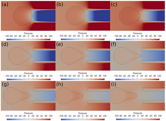
Figure 9.
Pressure contours around the clot after every ms. (a) Time ms, (b) time ms, (c) time ms, (d) time ms, (e) time ms, (f) time ms, (g) time ms, (h) time ms, (i) time ms. The initial distance between the clot and the catheter is 0.75 times the clot radius. Suction velocity is 0.2 m/s, flow velocity is −0.6 m/s. = 0.58, = 0.78, = 0. The pressure difference across the clot interface is strong only at the start of suction process; later, the pressure gradient diminishes as the clot moves away from the catheter tip.
4.2. Results Based on Viscoelastic Formulation
In this section, we present the results based on the viscoelastic formulation. Figure 10 shows the clot shapes filled with viscoelastic normal stress , Figure 11 shows the clot shapes filled with shear stress , and, finally, Figure 12 shows the clot shapes filled with normal stress after every seven milliseconds. As can be seen in the figures, the cloud thins out as it is sucked, and high viscoelastic stresses develop inside it. The clot finally ruptures inside the catheter during the later stages of suction. As can be noticed in the above mentioned figures, the magnitude of tensile stress is much larger (∼23 Pa) compared to that of (∼1.7 Pa) and (∼0.2 Pa). This is due to the stretching of the clot inside the catheter. In the next section, we conclude the current work.
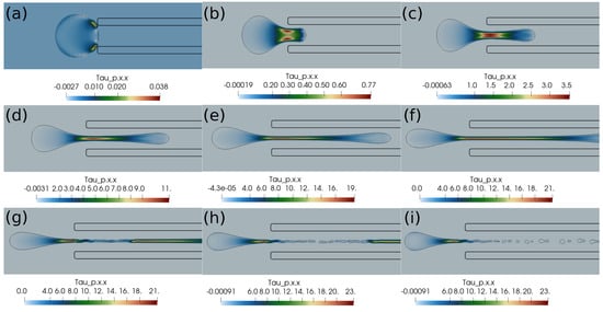
Figure 10.
Viscoelastic stress distribution inside the clot. (a) Time ms, (b) time ms, (c) time ms, (d) time ms, (e) time ms, (f) time ms, (g) time ms, (h) time ms, (i) time ms. The initial distance between the clot and the catheter is 0.75 times the clot radius. Suction velocity is 0.4 m/s, flow velocity is −0.6 m/s. The clot ruptures inside the catheter as it is pulled.
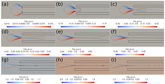
Figure 11.
Viscoelastic stress distribution inside the clot. (a) Time ms, (b) time ms, (c) time ms, (d) time ms, (e) time ms, (f) time ms, (g) time ms, (h) time ms, (i) time ms. The initial distance between the clot and the catheter is 0.75 times the clot radius. Suction velocity is 0.4 m/s, flow velocity is −0.6 m/s. The clot ruptures inside the catheter as it is being pulled.
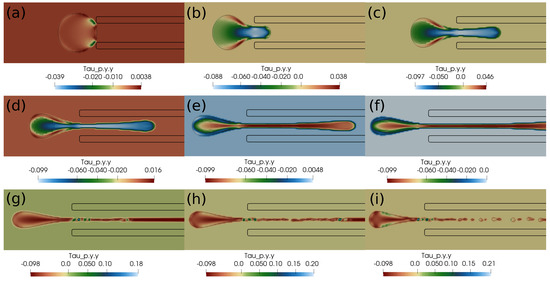
Figure 12.
Viscoelastic stress distribution in the clot. (a) Time ms, (b) time ms, (c) time ms, (d) time ms, (e) time ms, (f) time ms, (g) time ms, (h) time ms, (i) time ms. The initial distance between the clot and the catheter is 0.75 times the clot radius. Suction velocity is 0.4 m/s, flow velocity is −0.6 m/s. The clot ruptures inside the catheter as it is pulled.
5. Conclusions
To conclude the current work, we performed a direct numerical simulation of the clot extraction process using an aspiration-based thrombectomy technique. We assumed two different material models for the clot, namely, the hyperelastic and viscoelastic behavior models. We noticed an almost constant pressure difference of around 100 Pa across the clot in the clot-capturing case with a higher suction velocity. This pressure difference helps in the initial attraction of the clot towards the catheter tip. With lower suction velocity, the pressure difference across the clot keeps decreasing, which makes it impossible to induce clot suction. We also observed that the viscous stresses play a crucial role in the suction or escape of the clot. Once the clot is attracted towards the suction port of the catheter due to pressure difference, the viscous stresses shear the clot inside the catheter and hence help in its capture. On the other hand, if the clot is not attracted initially due to insufficient pressure difference, it is carried downstream by the viscous stresses due to the incoming blood flow. Therefore, the initial attraction stage is crucial for the suction or escape of the clot. We also observe that a higher suction velocity is, in general, helpful in capturing the clot. The results based on the viscoelastic formulation predict the rupture of the clot inside the catheter as the clot is being sucked. High values of tensile and shear stresses exist inside this clot during suction. The hyperelastic and viscoelastic models predict different behaviors of the clot during suction inside the catheter. Future work on the topic may include flow analysis of realistic, patient-specific geometries of cerebral blood vessels, modeling of contact forces between the clot and the catheter, and advanced material laws for clot dynamics.
Author Contributions
Conceptualization, S.V.; methodology, S.S.Y.; software, S.S.Y.; validation, S.S.Y.; formal analysis, S.V.; investigation, S.V.; resources, T.M. and S.K.K.; data curation, S.V.; writing—original draft preparation, S.V.; writing—review and editing, T.M. and S.K.K.; visualization, S.S.Y.; supervision, T.M. and S.K.K.; project administration, T.M. and S.K.K.; funding acquisition, T.M. and S.K.K. All authors have read and agreed to the published version of the manuscript.
Funding
This work is carried out as part of the research project (project ID: 2021-13255) titled “MeDiKiT: Medical Data Integration Toolkit—A Pilot Implementation of Medical Data Sharing Software Systems for Future Medicine to Enable Big Data & AI Applications in Medicine” sponsored by the Indian Council of Medical Research (ICMR), sanction no. BMI/12(40)/2022.
Data Availability Statement
The data related to the simulation work in this manuscript will be available on request.
Acknowledgments
The authors thankfully acknowledge the effort by Stephane Popinet while creating the open source flow solver Basilisk which was used for the simulation work presented in this manuscript.
Conflicts of Interest
The authors declare no conflicts of interest.
Nomenclature
| Conformation tensor | |
| Log conformation tensor | |
| Left Cauchy-Green deformation tensor | |
| Mooney-Rivlin material constants | |
| Tensor from decomposition of | |
| Tensor from decomposition of | |
| Rate of deformation tensor | |
| Identity tensor | |
| G | Shear modulus |
| Density | |
| Blood Density | |
| Clot Density | |
| Viscosity | |
| Blood Viscosity | |
| Clot Viscosity | |
| Polymeric Viscosity | |
| Clot fraction | |
| Hyperelastic stress | |
| Polymeric stresses | |
| p | Pressure |
| Relaxation time of polymer | |
| Velocity vector | |
| Time step | |
| D | Diameter of blood vessel |
| Clot diameter | |
| d | Catheter diameter |
| t | Time |
| Thickness of catheter wall | |
| Distance of clot from catheter tip |
References
- Johnson, W.; Onuma, O.; Owolabi, M.; Sachdev, S. Stroke: A global response is needed. Bull. World Health Organ. 2016, 94, 634. [Google Scholar] [CrossRef] [PubMed]
- Modin, D.; Claggett, B.; Sindet-Pedersen, C.; Lassen, M.C.H.; Skaarup, K.G.; Jensen, J.U.S.; Fralick, M.; Schou, M.; Lamberts, M.; Gerds, T.; et al. Acute covid-19 and the incidence of ischemic stroke and acute myocardial infarction. Circulation 2020, 142, 2080–2082. [Google Scholar] [CrossRef] [PubMed]
- Gralla, J.; Schroth, G.; Remonda, L.; Nedeltchev, K.; Slotboom, J.; Brekenfeld, C. Mechanical thrombectomy for acute ischemic stroke: Thrombus–device interaction, efficiency, and complications in vivo. Stroke 2006, 37, 3019–3024. [Google Scholar] [CrossRef] [PubMed]
- Rigatelli, G.; Cardaioli, P.; Roncon, L.; Giordan, M.; Milan, T.; Zonzin, P. Combined percutaneous aspiration thrombectomy and rheolytic thrombectomy in massive subacute vena cava thrombosis with ivc filter occlusion. J. Endovasc. Ther. 2006, 13, 373–376. [Google Scholar] [CrossRef]
- Kang, D.-H.; Hwang, Y.-H.; Kim, Y.-S.; Park, J.; Kwon, O.; Jung, C. Direct thrombus retrieval using the reperfusion catheter of the penumbra system: Forced-suction thrombectomy in acute ischemic stroke. Am. J. Neuroradiol. 2011, 32, 283–287. [Google Scholar] [CrossRef]
- Goh, G.S.; Morgan, R.; Belli, A.-M. Thrombolysis, mechanical thrombectomy and percutaneous aspiration thrombectomy. In Vascular Interventional Radiology: Current Evidence in Endovascular Surgery; Springer: Berlin/Heidelberg, Germany, 2012; pp. 89–99. [Google Scholar]
- Kim, S.K.; Yoon, W.; Moon, S.M.; Park, M.S.; Jeong, G.W.; Kang, H.K. Outcomes of manual aspiration thrombectomy for acute ischemic stroke refractory to stent-based thrombectomy. J. Neurointerv. Surg. 2014, 7, 473–477. [Google Scholar] [CrossRef]
- Patki, P.; Simon, S.; Manning, K.B.; Costanzo, F. Computational analysis of effects of clot length on acute ischemic stroke recanalization under different cyclic aspiration loading conditions. Int. J. Numer. Methods Biomed. Eng. 2023, 39, e3667. [Google Scholar] [CrossRef]
- Lally, F.; Soorani, M.; Woo, T.; Nayak, S.; Jadun, C.; Yang, Y.; McCrudden, J.; Naire, S.; Grunwald, I.; Roffe, C. In vitro experiments of cerebral blood flow during aspiration thrombectomy: Potential effects on cerebral perfusion pressure and collateral flow. J. Neurointerv. Surg. 2015, 8, 969–972. [Google Scholar] [CrossRef]
- Bungartz, H.; Lindner, F.; Gatzhammer, B.; Mehl, M.; Scheufele, K.; Shukaev, A.; Uekermann, B. Precice—A fully parallel library for multi-physics surface coupling. Comput. Fluids 2016, 141, 250–258. [Google Scholar] [CrossRef]
- Souli, M.; Benson, D.J. Arbitrary Lagrangian Eulerian and Fluid-Structure Interaction: Numerical Simulation; John Wiley & Sons: Hoboken, NJ, USA, 2013. [Google Scholar]
- Mittal, R.; Iaccarino, G. Immersed boundary methods. Annu. Rev. Fluid Mech. 2005, 37, 239–261. [Google Scholar] [CrossRef]
- Griffith, B.E.; Patankar, N.A. Immersed methods for fluid–structure interaction. Annu. Rev. Fluid Mech. 2020, 52, 421–448. [Google Scholar] [CrossRef]
- Zhao, H.; Freund, J.B.; Moser, R.D. A fixed-mesh method for incompressible flow–structure systems with finite solid deformations. J. Comput. Phys. 2008, 227, 3114–3140. [Google Scholar] [CrossRef]
- Sugiyama, K.; Ii, S.; Takeuchi, S.; Takagi, S.; Matsumoto, Y. Full eulerian simulations of biconcave neo-hookean particles in a poiseuille flow. Comput. Mech. 2010, 46, 147–157. [Google Scholar] [CrossRef]
- Jiang, G.-S.; Shu, C.-W. Efficient implementation of weighted eno schemes. J. Comput. Phys. 1996, 126, 202–228. [Google Scholar] [CrossRef]
- Sugiyama, K.; Ii, S.; Takeuchi, S.; Takagi, S.; Matsumoto, Y. A full eulerian finite difference approach for solving fluid–structure coupling problems. J. Comput. Phys. 2011, 230, 596–627. [Google Scholar] [CrossRef]
- Ii, S.; Sugiyama, K.; Takeuchi, S.; Takagi, S.; Matsumoto, Y. An implicit full eulerian method for the fluid–structure interaction problem. Int. J. Numer. Methods Fluids 2011, 65, 150–165. [Google Scholar] [CrossRef]
- Ii, S.; Sugiyama, K.; Takagi, S.; Matsumoto, Y. A computational blood flow analysis in a capillary vessel including multiple red blood cells and platelets. J. Biomech. Sci. Eng. 2012, 7, 72–83. [Google Scholar] [CrossRef][Green Version]
- Sugiyama, K.; Ii, S.; Shimizu, K.; Noda, S.; Takagi, S. A full eulerian method for fluid-structure interaction problems. Procedia Iutam 2017, 20, 159–166. [Google Scholar] [CrossRef]
- Farahbakhsh, I.; Ghassemi, H.; Sabetghadam, F. An immersed boundary method based on the kinematic relation of the velocity-vorticity formulation. J. Mech. 2015, 31, 171–181. [Google Scholar] [CrossRef]
- Farahbakhsh, I.; Paknejad, A.; Ghassemi, H. A full-eulerian approach for simulation of a system of fluid–rigid–elastic structure interaction based on the vorticity-stream function formulation. Fluid Dyn. Res. 2023, 55, 015505. [Google Scholar] [CrossRef]
- Farahbakhsh, I.; Ghassemi, H.; Sabetghadam, F. A one-continuum approach for mutual interaction of fluids and structures. J. Mech. 2015, 31, 745–755. [Google Scholar] [CrossRef]
- Shi, Y.; Cheshire, D.; Lally, F.; Roffe, C. Suction force-suction distance relation during aspiration thrombectomy for ischemic stroke: A computational fluid dynamics study. Phys. Med. 2017, 3, 1–8. [Google Scholar] [CrossRef]
- Tashiro, K.; Shobayashi, Y.; Ota, I.; Hotta, A. Finite element analysis of blood clots based on the nonlinear visco-hyperelastic model. Biophys. J. 2021, 120, 4547–4556. [Google Scholar] [CrossRef]
- Oyekole, O.; Simon, S.; Manning, K.B.; Costanzo, F. Modeling acute ischemic stroke recanalization through cyclic aspiration. J. Biomech. 2021, 128, 110721. [Google Scholar] [CrossRef]
- Mirakhorli, F.; Vahidi, B.; Pazouki, M.; Barmi, P.T. A fluid-structure interaction analysis of blood clot motion in a branch of pulmonary arteries. Cardiovasc. Eng. Technol. 2023, 14, 79–91. [Google Scholar] [CrossRef]
- Luisi, C.A.; Amiri, A.; Büsen, M.; Sichermann, T.; Nikoubashman, O.; Wiesmann, M.; Steinseifer, U.; Müller, M.; Neidlin, M. Investigation of cerebral hemodynamics during endovascular aspiration: Development of an experimental and numerical setup. Cardiovasc. Eng. Technol. 2023, 14, 393–403. [Google Scholar] [CrossRef] [PubMed]
- Popinet, S. Basilisk Flow Solver and Pde Library. 2020. Available online: http://basilisk.fr (accessed on 31 March 2025).
- Eng, W.S. Nonlinear Stiffness and Viscoelasticity of Inhibitor-Treated Blood Clots by Tensile Testing. Ph.D. Thesis, San Jose State University, San Jose, CA, USA, 2018. [Google Scholar]
- Weymouth, G.D.; Yue, D.K.-P. Conservative volume-of-fluid method for free-surface simulations on cartesian-grids. J. Comput. Phys. 2010, 229, 2853–2865. [Google Scholar] [CrossRef]
- López-Herrera, J.M.; Popinet, S.; Castrejón-Pita, A.A. An adaptive solver for viscoelastic incompressible two-phase problems applied to the study of the splashing of weakly viscoelastic droplets. J. Non-Newton. Fluid Mech. 2019, 264, 144–158. [Google Scholar] [CrossRef]
- The Log-Conformation Method for Some Viscoelastic Constitutive Models. Available online: http://basilisk.fr/src/log-conform.h (accessed on 31 March 2025).
- Bell, J.B.; Colella, P.; Glaz, H.M. A second-order projection method for the incompressible navier-stokes equations. J. Comput. Phys. 1989, 85, 257–283. [Google Scholar] [CrossRef]
- Popinet, S. Gerris: A tree-based adaptive solver for the incompressible euler equations in complex geometries. J. Comput. Phys. 2003, 190, 572–600. [Google Scholar] [CrossRef]
- Popinet, S. An accurate adaptive solver for surface-tension-driven interfacial flows. J. Comput. Phys. 2009, 228, 5838–5866. [Google Scholar] [CrossRef]
- Acceleration Term in a Hyperelastic Incompressible Material. Available online: http://basilisk.fr/sandbox/lopez/src/hyperelastic.h (accessed on 31 March 2025).
- Jain, S.S.; Kamrin, K.; Mani, A. A conservative and non-dissipative eulerian formulation for the simulation of soft solids in fluids. J. Comput. Phys. 2019, 399, 108922. [Google Scholar] [CrossRef]


Disclaimer/Publisher’s Note: The statements, opinions and data contained in all publications are solely those of the individual author(s) and contributor(s) and not of MDPI and/or the editor(s). MDPI and/or the editor(s) disclaim responsibility for any injury to people or property resulting from any ideas, methods, instructions or products referred to in the content. |
© 2025 by the authors. Licensee MDPI, Basel, Switzerland. This article is an open access article distributed under the terms and conditions of the Creative Commons Attribution (CC BY) license (https://creativecommons.org/licenses/by/4.0/).