Abstract
The flow of viscous and highly viscous fluids in straight and bent pipes and channels is a fundamental process in a wide variety of industrial applications and is, therefore, of great interest in science and engineering. Understanding the physics behind such flows has a direct impact on the design of efficient, safe and reliable systems. The type of fluid, which can be viscous or even highly viscous, and the pipe geometry can affect the flow dynamics, the pressure loss and the overall efficiency of the process. In this paper, we provide an extensive review of the state-of-the-art research concerning the flow of Newtonian and non-Newtonian, single-phase fluids in straight and bent pipes. Since a big amount of work in the literature is devoted to the study of Newtonian pipe flows, the paper starts with a brief outline of the nonlinear theory of viscous Newtonian fluid flow in pipes, including a survey of early and recent analytical solutions to the Navier–Stokes equations. The central part of the paper deals with an extensive overview of existing experimental and numerical research work on viscous Newtonian pipe flows. Separate sections are devoted to non-Newtonian fluid flows, the problem of entropy generation due to irreversible processes in the flow and hydromagnetic Newtonian and non-Newtonian pipe flow. The review closes with a brief survey of machine learning and artificial intelligence modeling applied to pipe flow along with future trends and challenges in pipe flow research.
1. Introduction
The movement of fluids in pipes and pipeline components, as well as its physical description in terms of the flow regimes encountered, is of fundamental importance in science and engineering. Several applications, such as household water and gas supply, sewage flows and numerous industrial processes, require the transportation of fluids through pipes. Although all fluids in nature are viscous, highly viscous liquids offer higher resistance to flow because of their stronger intermolecular forces, resulting in higher internal friction. This slows the movement of liquid layers past one another compared to low-viscosity liquids, which flow much more easily because of their corresponding lower friction forces. In spite of this difference between low- and high-viscosity fluids, a review of highly viscous fluid flows in pipes must in general cover the topic of viscous fluid flows in pipes and ducts.
Although the transport of water through pipes dates back to Roman times, the first scientific studies of flow through a pipe began in 1839, when Hagen [1] and then Poiseuille [2] performed the first experiments (reported in the literature) of laminar flow of water through straight pipes of various sizes to determine pressure losses. This flow is known today as the Hagen–Poiseuille flow. In particular, Hagen [1] first observed that above a certain pressure head the flow becomes unstable, undergoing a transition from laminar to turbulent state. Later, similar studies were carried out by Darcy [3], who also considered the effects of pipe roughness on pressure drop, and Reynolds [4], who observed that the transition to turbulent flow occurs above a certain critical value, known today as the critical Reynolds number. The Reynolds number (Re) measures the relationship between the inertial forces and the viscous forces present in the fluid and is used to indicate whether the flow is laminar or turbulent. On the other hand, the friction factor, which relates the pressure drop to the flow velocity and the roughness of the pipe, and the energy losses have an important impact on flow efficiency and performance. Early studies also focused on investigating the flow through curved pipes [5,6,7,8,9,10,11], revealing that (1) the curvature balance between pressure and centrifugal forces in a bend leads to the formation of a secondary flow there, often in the form of two symmetrical vortices, (2) the maximum flow velocity due to this imbalance in fluid motion occurs toward the outer pipe wall at the outlet of the bend, (3) the pressure losses are greater than in straight pipes and (4) the critical Reynolds number for transition to turbulent flow increases compared to straight pipes. In addition, Dean [12,13] studied the centrifugal instabilities in curved pipes and showed by analytical means that the emerging secondary flow is characterized by two counter-rotating vortex cells, which are known today as Dean vortices. In particular, these early studies have provided the basis for the current theory of pipe flow. The emergence of turbulence in straight and curved pipe flows has been thoroughly reviewed by Kalpakli Vester et al. [14], while a comprehensive review of advances in experiments and simulations of fluid flow in helically coiled pipes has been recently presented by Sigalotti et al. [15].
Single-phase viscous flow in pipes can be laminar (i.e., smooth and steady) at low Re, in a transition state from laminar to turbulent at intermediate Re values, and turbulent (i.e., fluctuating) at high Re. The type of regime encountered will depend on the pipe geometry (i.e., the pipe bending, which can be sharp or moderate, and the cross-sectional area, which can be circular, square, elliptical, rectangular, etc.), the fluid properties and the flow parameters of the system as well as the roughness and rigidity of the pipe wall. In addition to the need to redirect the flow through curved sections, many pipeline systems may have branches and junctions that serve to distribute the flow. This is the case of the transportation of oil and gas in pipelines from the production well to the refining plant, cold water in the refrigeration system of nuclear reactors, air in the respiratory system and blood in the cardiovascular system of mammals, non-Newtonian fluids during food processing operations, among many other processes. Whereas liquids are in general incompressible, the transportation of gas (and air) will require to consider the effects of compressibility. The above discussion shows how the flow regime depends on several conditions, which in general complicates the correct description of the flow in pipes and pipeline systems and components.
The flow of viscous fluids in straight and curved pipes has been the subject of extensive theoretical and experimental research since the early investigations carried out by Hagen [1] and Poiseuille [2]. There are several books and review articles and a huge amount of research articles dealing with the flow of viscous fluids through straight and curved pipes under various conditions that have been published during the last ninety years, spanning from 1938 to 2024 [14,15,16,17,18,19,20,21,22,23,24,25,26]. Citations to a large number of research articles dealing with laminar and turbulent viscous flow through pipes and ducts will be made throughout the text in the following sections. The focus of the present review article will be on viscous and highly viscous single-phase flows through straight and curved pipes, including only pipe bends and elbows, based on experiments and numerical simulations. For a recent review of flow through helically coiled pipes, the interested reader is referred to Ref. [15]. As mentioned above, the turbulent flow through straight and curved pipes along with a historical background spanning from 1839 to 2016 has been reviewed by Kalpakli Vester [14]. Therefore, in addition to a short review of the material covered by Kalpakli Vester et al. [14], we will expand more on the experimental and numerical work performed over the last two decades.
For reasons of space, the flow in micro-devices, such as channels and heat pipes, as well as in nanotubes, was not considered in the present review. In the last 20 years, the research in the field of micro-fluidic has been constantly increasing due to the very rapid growth of technological applications that require heat transfer in miniature volumes. In the same way, the transport of nanofluids in mini- and micro-channels has been pointed out as a promising candidate for a disproportionate enhancement of heat transfer in important engineering applications, including energy storage, electronics cooling and the thermal processing of materials. This has generated a huge amount of published papers that a comprehensive review of the subject will require writing a separate paper. However, the interested reader is referred to recent comprehensive reviews by Singh and Myong [27], Kavokine et al. [28] and Zhang et al. [29] of flow in nano-, micro- and mini-channels. In passing, we note that Inamdar and Lawankar [30] have also published a recent review dealing with flow boiling in micro- and mini-channels.
The paper is organized as follows. The basic parameters, definitions and friction factor correlations for the prediction of frictional pressure losses that characterize the flow of Newtonian fluids through a pipe are described in Section 2. A brief outline of the nonlinear theory of viscous Newtonian fluid flow in pipes is given in Section 3. Section 4 and Section 5 deal with an overview of experimental work and results obtained from numerical simulations of Newtonian fluid flows in pipes, respectively. The flow of non-Newtonian fluids in pipes and ducts is reviewed in Section 6. The problem of entropy generation in pipe flows is discussed in Section 7. Section 8 provides a brief survey on hydromagnetic flows in pipes. Section 9 contains a brief overview of the rapid development of machine learning and artificial intelligence in pipe flow research, while Section 10 contains a brief outline of possible directions for future research and challenges. Finally, Section 11 summarizes the main conclusions.
2. Useful Parameters and Friction Factor Correlations for Newtonian Fluid Flow in Pipes
2.1. Basic Parameters
A fundamental parameter in fluid mechanics is the dimensionless Reynolds number defined as
where is the fluid density, v is the mean flow velocity, l is some characteristic length scale related to the flow and is the shear viscosity coefficient of the fluid. This parameter measures the importance of inertial forces over viscous forces. For fluid flow in a pipe, the Reynolds number is often written in terms of the pipe diameter, D, and the kinematic viscosity, , as
In particular, Reynolds [4] showed experimentally that the transition from laminar (low Re) to turbulent (high Re) flow in a pipe of circular cross-sectional area occurs at a critical Re-value of . In the laminar regime small disturbances in the flow are quickly damped, while at the transitional regime, the flow is characterized by intermittent bursts of turbulence. It is frequently found in the literature that the approximate range is characteristic of the (creeping) motion of highly viscous fluids, while for , the flow is still laminar but with a rather strong Re-dependence. In the interval, a transition to turbulence can be observed, and, only for , the flow becomes turbulent. However, these ranges are only representative and can vary depending on the flow geometry, the pipe wall roughness and the level of fluctuations in the inlet stream.
For curved pipe flows, a relevant dimensionless parameter is the Dean number [12,13]
where is the curvature ratio, R is the pipe radius and is the radius of curvature, defined as the distance from the center of curvature to the centerline of the pipe. For straight pipes, ; therefore, , while for sharp bends (i.e., elbows), since, in this case, . From the entrance region of a pipe, there is a finite distance beyond which the flow becomes fully developed; that is to say, the flow streamwise velocity profile becomes invariant. For fully developed laminar flow, this finite distance can be estimated using the empirical correlation
For turbulent flow, this distance is relatively shorter and can be estimated from the correlation
2.2. Friction Factor Correlations
A dimensionless quantity that relates the pressure losses to the square of the streamwise velocity is the so-called Fanning friction factor given by
where is the pressure gradient along the pipe. As a fluid flows through a pipe, its interaction with the pipe walls produces friction, which in addition to reducing the pressure along the pipe slows down the flow. Therefore, the Fanning friction factor is a key parameter used to estimate pressure losses in a pipe. The Darcy–Weisbach factor, defined as , is often used to describe friction losses in laminar and turbulent flows in pipes and open channels. From now on, we will refer to the Darcy–Weisbach friction factor simply as the friction factor and use F rather than to denote it. For laminar (smooth) flow in a circular pipe of diameter D, the friction factor is . Note that for pipes with non-circular cross-sections, D is replaced by the hydraulic diameter, , in the definition of Re, where A is the cross-sectional area of the flow and P is the wet perimeter of the pipe cross-section.
The dependence of the friction factor on Re has been used as an indicator of whether the flow is laminar, transitional or turbulent. Therefore, the friction factor is not a constant, and, in the same way as Re, it depends on the pipe characteristics, the flow velocity and the type of fluid. In general, it can be estimated from empirical correlations or it can be read from Moody diagrams [31], where the friction factor is plotted as a function of Re. In the turbulent regime, the friction factor varies slowly with Re between and 0.06, and the flow can be divided into sub-regimes depending on whether the pipe wall is smooth or rough. For turbulent flow in smooth pipes, the transfer of momentum from the bulk of the fluid to the pipe wall is governed by many small eddies; therefore, the friction factor can be estimated solving the transcendental equation, referred to as the Kármán–Prandtl resistance equation [32]
where the constant factors are chosen to provide a fairly good fit to the data [33]. Using the Lambert W function, Equation (7) can be written in the more compact form
For flow through a pipe with rough walls, the friction factor differs from the smooth pipe curve and approaches an asymptotic value, known as the rough pipe regime. When the height of the wall roughness, , is important, a number of existing correlations for the friction factor are given in terms of the modified Reynolds number [34]
which is often referred to in the literature as the roughness friction Reynolds number.
Figure 1 shows the roughness function B as a function of for different values of the roughness ratio between 0.00006 and 0.033 (colored dots) and the functions predicted by Colebrook [35] and Afzal [36] (solid lines). The dots include data flow measurements reported by Nikuradse [34], Shockling et al. [37] and Langelandsvik et al. [38] for a commercial steel pipe. In the region , the roughness function varies linearly with . This region describes the smooth pipe regime. In the interval , the data slowly deviate from linear, reaching a maximum value around and then monotonically decreasing to a constant value at . This interval describes the transition from smooth to rough pipe flow. At , the roughness function approaches asymptotically a constant value and becomes almost independent of and .
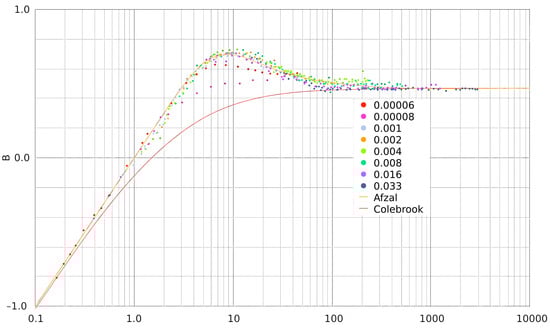
Figure 1.
Dependence of the roughness function B on the friction Reynolds number . The solid lines depict the functions predicted by Colebrook [31] and Afzal [32]. Figure credit: Arthur Ogawa. Figure adapted from https://commons.wikimedia.org/wiki/File:Figure3(BvsR*).svg#file (accessed on 7 February 2025).
For turbulent flow in transitional rough pipes, Afzal and Seena [39] have introduced the inner rough wall variable , where is a transitional roughness scale such that all mean relative motions and energy components of the turbulent flow are independent of the surface roughness. In terms of , the roughness Reynolds number can be defined as [36,39]. Note that for , . For transitional roughness in pipes, Afzal [36] reports the friction factor relation in terms of
which has been adjusted to match Prandtl’s [40] smooth wall relation. In the range , this relation describes very well the fully smooth pipe data of Nikuradse [34]. Based on Princeton’s superpipe data of McKeon [41] for , the alternate correlation for transitional pipe roughness is given by [36]
For inflectional roughness, the friction factor in terms of and based on Prandtl’s [40] smooth wall relation becomes [36]
while based on smooth pipe constants from McKeon [41], the friction factor in terms of becomes
In relations (12) and (13), the value of j is set to 11 to better describe the transition from a smooth to a rough pipe regime [36,39]. For transitional rough pipes, alternate forms of Equations (12) and (13) are listed in Table 1 of Ref. [36] for different roughness parameters. Since these equations are implicit in nature, they must be solved iteratively. However, each of them can be manipulated in an explicit expression that allows one to calculate the friction factor approximately (see Table 1 of Ref. [36]). Alternative formulas to Equations (12) and (13) due to machine honed surface roughness in fully developed turbulent flow were further proposed by Afzal et al. [42] to be
where was used to fit the data of Nikuradse [34].
The correct behavior at can be reproduced using the Colebrook–White relation [35]
According to Figure 1, this relationship approximates the behavior for the smooth pipe regime at and substantially underestimates the friction factor in the transitional domain [37]. Several authors have proposed approximations to Equation (14) for turbulent flow through circular pipes [43,44,45,46,47,48]. A list of available Colebrook–White based explicit friction factor relations can be found in Ref. [48]. In particular, Serghides’s [45] solution was found to be one of the most accurate, matching the Colebrook–White implicit solution within an error of about 0.0023%. More recently, Niazkar [48] developed a modified version of the Serghides’s solution, which is known to be the most accurate approximation to the Colebrook–White implicit formula. For fully rough pipes, Afzal [36] proposed the following explicit counterpart relations to Equations (14) and (15), respectively:
Friction factor correlations for laminar and turbulent viscous flows in helical pipes have been reviewed recently by Sigalotti et al. [15]; therefore, they will not be repeated here. Other parameters of interest in the description of certain flow cases will be introduced in conjunction with their discussion in the next sections.
3. Theory of Viscous Newtonian Fluid Flow in Pipes
3.1. Governing Equations
The motion of a viscous fluid in a pipe is described by the physical laws of mass, momentum and energy conservation. These can be written in terms of a set of coupled nonlinear differential equations, which in Lagrangian coordinates have the form
where is the fluid density, is the fluid velocity vector, U is the fluid specific internal energy, is the gravitational acceleration vector, is the stress tensor given by
and is the heat flux vector, defined as
In Equations (21) and (22), p denotes the pressure, the shear viscosity coefficient, the bulk viscosity, d the dimension factor, the unit tensor, the heat conductivity and T the fluid temperature. Sometimes requiring that the second law of thermodynamics be satisfied, the entropy balance equation
must be solved coupled to Equations (18)–(20), where S is the specific entropy and
is the entropy production due to the irreversible processes of frictional viscous dissipation and heat transfer. Under non-isothermal effects, the above differential equations must be solved coupled to pressure, , and caloric, , equations of state. In general, appropriate boundary conditions require setting at the pipe wall.
For incompressible fluids, such as most liquids, Equation (18) simplifies to , and Equation (19) takes the form of the Navier–Stokes equations
In the presence of heat transfer, the specific internal energy equation becomes
Sometimes Equation (26) is converted into a temperature equation by setting , where is the specific heat at constant pressure.
3.2. Analytical and Semi-Analytical Approaches
In their very recent comprehensive review of 2023, Urbanowicz et al. [49] classified the analytical solutions to the Navier–Stokes equations for the laminar accelerated flow of viscous Newtonian fluids in a pipe into two main groups, where the first group, which is made up of classical (earlier) solutions, deals with models of flow acceleration driven by a step pressure gradient along the length of the pipe, while in the second group of solutions, which appeared in the literature more recently, the flow motion is forced by imposition of a flow rate. These latter models include solutions for the laminar flow of viscous fluids in a porous pipe. However, in the next sections, we will refer to “classical solutions” as those that were reported in the literature before the end of the last century, which may include both groups of solutions, and to “more recent solutions” as those solutions that were reported later.
3.2.1. Classical Exact Solutions
Complete exact solutions to the Navier–Stokes equations for fluid flow in a pipe can be derived only for cases in which the non-linear terms can be neglected. As quoted by Urbanowicz et al. [49], the first known analytical solution to the Navier–Stokes equations for the accelerated flow of an incompressible viscous fluid in a vertical hydraulic pipe was presented in 1871 by the Italian physicist Antonio Roiti [50] at the University of Pisa. On the other hand, a similar analytical solution for horizontal pipes was obtained by the Russian physicist Ippolit S. Gromeka in 1882 [51]. As was pointed out by Urbanowicz et al. [49], these two solutions were not noticed for a long time until they were revealed to the scientific community in relatively recent times. Examples of classical solutions for the velocity field, which are described in many introductory books on Fluid Mechanics, are the several variants of laminar Poiseuille flow [52], including the famous time-dependent plane Poiseuille and Hagen–Poiseuille flow in a pipe [53], the steady-state Poiseuille flow in an annular section [54] and through pipes of non-circular cross-sectional area [5,55,56,57], the unsteady Poiseuille flow with an oscillating pressure gradient [58,59], the Couette flow of a viscous fluid between two surfaces when one slides over the other [60] and the Taylor–Couette flow between two rotating and infinitely long coaxial cylinders [61]. A steady-state solution also exists for the Taylor–Couette flow between two finite-length rotating cylinders [62]. A further notorious exact solution of the Navier–Stokes equation is the so-called Stokes problem or Stokes boundary layer, which consists in finding a solution for the flow induced by an oscillating solid surface [63].
Possibly the most celebrated flow solution is the time-dependent Hagen–Poiseuille flow, which describes the movement of a viscous fluid along a cylindrical pipe of constant inner diameter driven by a step pressure gradient. In this case, the solution can be derived for initial conditions, corresponding to a fluid initially at rest (i.e., ), and no-slip boundary conditions at the pipe wall due to the effects of viscosity. After a transient, a steady-state solution, corresponding to a parabolic velocity profile, is achieved, where the peak velocity occurs along the axis of symmetry () of the pipe. Using cylindrical coordinates () to represent the flow and leaving aside the details of the derivation, the exact solution for the Hagen–Poiseuille flow through a pipe of radius R is given by
where is the maximum asymptotic velocity, which is proportional to the hydrostatic pressure difference () between the two ends of the pipe of length L, is the kinematic viscosity, the (with ) are the Bessel functions of the first kind of integral order n, and (for are the roots of . A generalization of the above solution for a non-vanishing initial velocity, starting with a steady-state Hagen–Poiseuille profile, and a step change pressure gradient was reported by Ito [64]. This author also developed an exact solution for a time-varying pressure gradient (see Ref. [64]).
Almost all analytical solutions of the Hagen–Poiseuille type assume that the pressure gradient varies steeply from an initial to a final value. This differs from real systems where the pressure gradient does not vary steeply since it depends on the valve opening time [49]. In particular, Avula [65] and Avula and Young [66] demonstrated by experimental means that, in real systems, the flow velocity varies with time differently as stated by the classical Hagen–Poiseuille theory and provided a modified semi-analytical solution for the velocity profile. The discrepancy in the velocity profiles with the classical theory is greater at the beginning of the transient stage and becomes considerably smaller at larger times. A further generalization of the Hagen–Poiseuille flow for a time-varying pressure gradient of the form was obtained in 1997 by Smith [67], where k and b are positive constants, and r and z are cylindrical coordinates. For a pipe of radius and taken the fluid at rest for with the pressure gradient turned on at , Smith’s [67] exact solution reads as follows
where (with ) are the roots of . In passing, we note that universal solutions for arbitrary pressure gradients were obtained by a number of authors [68,69,70,71,72,73,74,75,76] and more recently by Lee [77], which include flows under sinusoidal pressure gradients.
Analytical solutions to the Navier–Stokes equations for laminar flow in a long pipe can also be obtained by imposing a flow rate. The idea of assuming a constant flow rate was first considered by Andersson and Tiseth [78], who obtained the exact solution for laminar flow along a cylindrical pipe of radius a
where , and are dimensionless variables defined by , and , is twice the final mean flow velocity and is the mth zero of the Bessel function for . Figure 2 shows the temporal evolution of the velocity profiles as calculated from Equation (29). A parabolic velocity profile is established at , much earlier than for the Hagen–Poiseuille flow given by Equation (27) for the same pipe configuration. A solution identical in form to Equation (29) was previously derived by Sparrow et al. [79] by assuming a pressure inlet from a reservoir at the pipe entrance. The only difference is that the dimensionless time, , in Equation (29) is replaced by a dimensionless distance , where is a stretched axial coordinate, a is the radius of the cylindrical pipe and is the mean velocity. Das and Arakeri [80] derived an analytical solution for the case when the imposed flow rate is caused by a piston motion at the entrance of the pipe. In this case, the solution for the flow velocity is a piecewise function: (a) for flow acceleration from rest, (b) for flow driven by a constant piston velocity, (c) for flow during piston deceleration and (d) for flow to rest when the piston is stopped. Figure 12 of Ref. [49] shows the course of Das and Arakeri’s [80] solution over time as compared to Andersson and Tiseth’s [78] model solution for a constant flow rate.
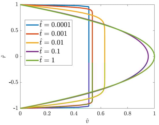
Figure 2.
Streamwise velocity profiles at selected times as predicted by Equation (29) for the accelerated laminar flow driven by a suddenly imposed constant flow rate. Figure taken from Urbanowicz et al. [49].
An analytical axisymmetric solution for laminar flow in a porous cylindrical tube was obtained by Terrill [81] by superposing potential flow on the Poiseuille flow. In order to overcome the difficulty that sometimes a fully developed velocity profile cannot be achieved due to a fluid long memory of the inlet velocity profile for constant suction (or mass injection) at the wall [82], he introduced a solution for the case of variable mass transfer at the pipe wall. Later, this solution was extended to the case of flow along pipes with impermeable walls and varying circular cross-sectional area by Terrill and Colgan [83]. In this case, analytical solutions to the Navier–Stokes equations with appropriate boundary conditions were obtained by expanding the potential function into a power-series expansion of the cylindrical coordinates z and r up to quadratic and cubic order. An analytical solution for fully turbulent, incompressible flow in smooth pipes was also reported by Zagustin and Zagustin [84]. As these authors themselves commented, a remarkable property of this solution is that it depends only on the von Kármán universal constant. They reported solution curves for the mixing length, velocity and eddy viscosity distributions that are in excellent agreement with experimental data everywhere within the pipe. A particular class of flow solutions, i.e., the generalized Beltrami flows, which satisfy the condition , where is the vorticity, have been reviewed by Wang [85] for several types of flows, including the axisymmetric flow in a cylindrical porous pipe. Second-order solutions for the velocity, pressure and temperature, corresponding to flow of high viscosity in a long cylindrical tube, were obtained by Thomann [86] as functions of increasing powers of the Mach number for small shear wave numbers, , and the Prandtl number
where R is the pipe radius, is the frequency, and is the specific heat at constant pressure. These solutions were used to show that thermal effects (i.e., heat transferred to the pipe wall) in an incompressible liquid are an order of magnitude larger than in a gas.
3.2.2. Recent Analytical Solutions
The generalization of the Hagen–Poiseuille flow for vertical and sloping pipes was developed by Urbanowicz et al. [87]. They presented a universal solution that works for horizontal as well as for vertical and sloping (upward and downward) pipe flows. In terms of piezometric heads, the solution for the velocity reads as follows
where R is the inner pipe radius, L is the pipe length, is the inclination pipe angle measured with respect to an horizontal axis () and is the mth zero of the Bessel function . In this case, the shear stress on the pipe wall, , and the instantaneous coefficient of resistance, F, obey the exact expressions
where with . For , Equations (31)–(33) reduce to the Gromeka–Szymański solution [51] for flow in a horizontal pipe, while for and , they reduce to the form derived by Roiti [50] for upward and downward flow in a vertically oriented pipe. For , upward flow occurs when and downward flow otherwise. For angles in the interval , there will always be downward flow.
In a very recent study, Kanuri et al. [88] explored the interaction between the Poiseuille flow, the Coriolis force and the channel inclination in the fully developed flow of an incompressible viscous fluid for the case when the channel rotates with angular velocity perpendicular to the main flow. They found an analytical solution for the steady-state flow velocity given by
where the mainstream flow is along the x-direction, is the width of the channel, is the inclination angle of the channel measured with respect to an horizontal axis and . This solution describes a parabolic velocity profile with the maximum velocity along the centerline of the channel (). Figure 3 shows the response of the velocity to decreasing pressure gradient (left plot), to increasing rotation (middle plot) and to increasing inclination angle (right plot) from (perfectly horizontal) to (perfectly vertical). In the core of the channel, the mainstream velocity increases with decreasing pressure gradient and increasing rotation and inclination angle. The analytical solution for the axial and circumferential velocity of the unsteady flow of a viscous incompressible fluid as induced by the sudden swirling of a cylindrical pipe wall and starting with an axial velocity component was presented by Bocci et al. [89]. Moreover, Pillai and Manu [90] obtained time-dependent velocity profiles and pressure gradient for laminar flow in cylindrical pipes driven by an arbitrary flow rate with slip boundary conditions at the wall. In particular, they presented exact solutions for starting, oscillatory and arbitrary inflows.
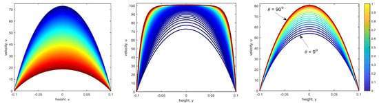
Figure 3.
Streamwise velocity profiles as predicted by the steady-state solution given by Equation (34) for incompressible flow of a viscous fluid in a rotating inclined channel. Response of the flow velocity with decreasing pressure gradient (left), increasing rotation (middle) and increasing inclination angle (right). Figure taken from Kanuri et al. [88]. http://creativecommons.org/licenses/by/4.0/ (accessed on 8 February 2025).
A standard problem in fluid dynamics concerns the laminar entrance flow in a cylindrical pipe, which precedes the fully developed Poiseuille flow. Recently, Kim [91] identified for the first time by analytical means the existence of velocity overshoot at a short distance from the pipe inlet, which is characterized by the maximum inflow velocity appearing near the pipe wall instead of the central symmetry axis as was corroborated by experimental measurements. Figure 4 shows a schematic drawing of the velocity evolution as predicted by Kim’s [91] analytical solution. The velocity overshoot is evident at the pipe entrance and progressively disappears as the velocity profile approaches a fully parabolic shape. Their Figures 3 and 4 show how well their predicted axial variation of the central axial velocity and pressure drop fits published experimental data. Based on the assumption of constant flow, , and a linear Navier slip boundary condition, , through the wall of a cylindrical pipe of radius oriented along the z-coordinate axis, where is the slip length, Cox and Hill [92] derived two approximate analytical solutions for the radial and axial velocity fields, namely, and
respectively, for fully developed laminar flow, where is a constant factor. They found that a second flow arises, which gives rise to enhanced flow rates compared to the conventional Poiseuille flow that occurs for an injected radial flow velocity across the permeable pipe wall boundary. However, as Cox and Hill [92] pointed out, such high flow rates do not explain the much higher rates that have been reported for carbon nanotubes.
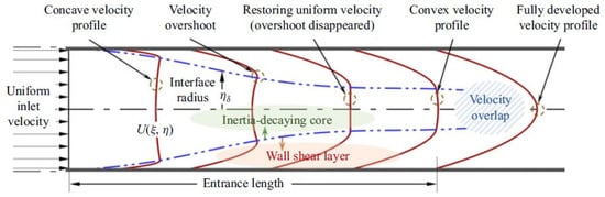
Figure 4.
Schematic drawing showing the development of the laminar entrance flow in a cylindrical long pipe as predicted by Kim’s [91] analytical solution. The presence of a velocity overshooting is evident near the pipe entrance. The velocity profiles are depicted in red, while the dash-double-dotted blue lines indicate how the the velocity overshooting is disappearing as the flow becomes fully developed. Figure taken from Kim [91].
As an additional interesting case, Kannaiyan et al. [93] derived an analytical solution for unsteady incompressible laminar flow in a cylindrical pipe subjected to arbitrary change in flow rate. They found solutions for the main velocity, pressure gradient, wall shear stress and skin friction factor when the flow rate changes in a step-like fashion from an initial value to a final value at an arbitrary time. Recently, Dunnimit et al. [94] obtained an approximate analytical solution for the time-fractional Navier–Stokes equations using the generalized Laplace residual power series method. They showed that by increasing the fractional order of the Katugampola fractional derivative of the Caputo type, the velocity of the fluid flow in a pipe is reduced. However, an increase in the radius of the pipe or the duration of the flow over time will increase the flow velocity. An explicit expression for the flow velocity was derived by Lyberg and Tryggeson [95] by considering the generation of vorticity at the boundaries of the system. They reformulated the Navier–Stokes equations in a divergence form that permitted immediate integration, allowing the velocity to be explicitly calculated and depend on boundary conditions only. Analytical solutions that aim to describe the flow of incompressible peristaltic viscous fluid in a horizontal tube were also presented by Mohammadein et al. [96,97].
Fatsis et al. [98] reported a new class of analytical solutions to the Navier–Stokes equations for unsteady swirling flow along a porous cylindrical tube rotating about its axis of symmetry. They found that the axial velocity peaks at the center of the pipe and decays toward its porous wall. In a more recent work, Manopoulos et al. [99] derived a generalized analytical solution for the laminar, oscillatory, creeping flow of an incompressible Newtonian fluid in a leaky pipe. In this case, suction and injection through the permeable wall of a cylindrical pipe of radius and aligned with the z-axis are represented by a spatiotemporal radial velocity of the form with period and amplitude . Using no-slip boundary conditions for the axial velocity, i.e., , Manopoulos et al. [99] obtained the following analytical solutions for the radial and axial velocities
where , , , and and are the zeroth- and first-order modified Bessel functions of the first kind, respectively. They examined their analytical solutions for varying Womersley numbers,
and ejection/suction parameters, , finding that the flow velocity decreases with increasing for all values of , while for small , the pressure increases. The same occurs when the ejection/suction frequency, , increases, which also leads to a shift of the peak velocity toward the leaky pipe wall. This mathematical model has important applications to the study of biofluidic systems, such as the renal tubules and the glymphatic system in the brain, where the leakage of fluids takes place across permeable interfaces.
Exact and approximate analytical solutions for the turbulent flow in a pipe are based on the idea that the flow velocity can be treated as the superposition of a turbulent (fluctuating) component on a laminar (parabolic) solution [100]. This kind of pipe flow was studied by García García and Alvariño [101], who solved analytically the Reynolds-averaged Navier–Stokes (RANS) equations for unsteady incompressible flow of a viscous fluid in a cylindrical pipe. In this approach, the mean field velocity is the sum of two components, namely, a laminar component, which is the result of a Poiseuille-type flow driven by the pressure gradient, and a turbulent one due to the Reynolds shear stress gradient developing within the pipe. A third component related to a transient response to the initial conditions disappears quickly. More recently, Fedoseyev [102] derived an approximate analytical solution to the so-called Generalized Hydrodynamic Equations (GHEs) for incompressible viscous flow. These equations are [103]: the continuity equation
and the momentum equation
where , is a scale velocity, L is the hydrodynamic length scale, is a body force and is a dimensionless time scale. The right-hand side of Equation (40) is the divergence of the fluctuating component of the velocity. The solution of Equations (39) and (40) allows explaining the nature of turbulence as the linear superposition of a laminar and a turbulent (super-exponential) solution
where is a parameter to be determined from experimental data, and . This analytical solution was found to compare well with experimental data for water flow in a horizontal pipe at and provided a complete structure of the turbulent boundary layer for experiments with distilled water flow at . A basic theory of viscous fluid flow in straight and curved pipes of circular and elliptical cross-section, which is valid for both incompressible and compressible linear viscous fluids, has been developed by Green and Naghdi [104] and Green et al. [105]. Explicit formulations of the mass flow rate per unit area, , for the compressible laminar and turbulent flow through a pipe were derived by Hullender et al. [106] in terms of empirical friction factors for both types of flow.
4. Experimental Studies: Flow of Newtonian Fluids in Pipes
In this section, we first perform a survey of early experimental studies, spanning the period from 1839 to 2000, whose results form the foundations on which the current theory of pipe flow is based. Experimental studies from the year 2000 onward will be reviewed separately in the following subsection.
4.1. Early Experimental Studies
The first experiments of fluid flow in pipes were largely restricted to measurements of pressure losses and to a very minor extent to flow visualization [1,2,3,4,6,7]. Two important conclusions were drawn from these early experiments, namely, that the laminar flow in a straight pipe becomes turbulent above a certain pressure head and that a secondary (circulatory) flow arises in a pipe bend, which occupies its entire cross-sectional area. Experiments mainly on water flow in curved pipes were continued in the early 1900s, with the work of Williams [8], who demonstrated for the first time that the point of maximum mean velocity at the exit of a bend shifts toward the outer wall of the pipe. Later, Eustice [9,10] found from similar experiments that the pressure drop in curved pipes was always greater than in straight pipes. However, Eustice also observed that the pressure changes in straight pipes at the transition point from laminar to turbulent flow did not occur so abruptly. Similar experiments were later taken up by White [11], who demonstrated by pressure drop measurements that the critical Reynolds number is generally much higher for curved pipes than for straight pipes. On the other hand, experiments by Taylor [107] showed that with increasing curvature, the transition from laminar flow to turbulent flow occurred for ever larger Reynolds numbers. The fully developed turbulent flow in a curved channel of constant curvature and cross-section was then experimentally studied by Wattendorf [108]. Measurement techniques include mainly laser Doppler velocimetry (LDV), hot-wire anemometry (HWA) and, in minor extent wall shear gauges, Pitot tubes and pressure taps. In particular, HWA measurements of velocity distributions downstream of pipe bends of circular, elliptical, square and rectangular cross-sectional area were presented by Weske [109]. In spite of differences in the cross-sectional shape, he found that the velocity distributions are quite similar and that the secondary flow arises as a consequence of the upstream flow converging asymmetrically with respect to the plane of the bend curvature. In addition, Detra [110] performed measurements of the mean axial velocity at through pipe bends of and , corresponding to curvature ratios and 0.04, respectively. Moreover, Tunstall and Harvey [111] found experimentally that turbulent flow through an L-shaped bend of circular cross-section produces a downstream secondary flow that is dominated by a single circulation instead of two counter-rotating Dean vortices, as usually found in pipe bends. For experimental data on measurements of pressure wall and pressure probe surveys prior to 1970, the interested reader is referred to the thorough review by Ward Smith [112] and references therein.
The development of the laser-Doppler anemometer has allowed for more detailed measurements of complex flows in pipes, including those occurring in bends and elbows. Therefore, after 1970, most experimental research has focused mainly on studying laminar and turbulent flows through curved pipes, in general. Humphrey et al. [113] studied experimentally the developing laminar flow of water through a bend of mm2 square section with smooth walls and long upstream and downstream ducts attached. They used laser-Doppler anemometry to provide measurements of longitudinal velocity and flow visualization for a qualitative analysis of the flow characteristics. Later, this study was extended to the analysis of turbulent flow using the same experimental setup used in the laminar flow analysis [114]. In this case, detailed measurements of the longitudinal and radial velocity components along with the corresponding components of the Reynolds stress tensor were provided using LDV techniques. Similar measurements of laminar and turbulent flows with thin inlet boundary layers using LDV methods were contemporaneously reported by Taylor et al. [115]. Other authors have performed experimental work on the development of turbulent flow in curved ducts with square and rectangular cross-sections [116,117,118,119]. In particular, Enayet et al. [117] found that for moderately curved ducts of square cross-section, the secondary cross-stream velocities are only one-half of those measured in strongly curved bends.
Further LDV measurements of laminar (at and 1093) and turbulent (at = 43,000) water flow in a circular cross-sectional bend were reported by Enayet et al. [120]. A schematic of their experimental test bend is shown in Figure 5. Their experimental model and results represent a benchmark for testing the accuracy of numerical simulations of laminar and turbulent flow in pipe bends. Long straight pipes of length 240 mm and 480 mm were attached upstream and downstream of the bend, respectively, and the entire system fitted to a closed-loop water flow rig. For flow field visualization, they used a laser light beam focused onto a radial diffraction grating. The beam was collimated to reduce spherical aberration and focused to form the scattering volume at the measurement point in the bend. Measurements were made by turning the light beam through using an optically flat mirror. The forward scattered light that was collected by an objective lens was focused on and passed through a pinhole to a photomultiplier. The output signal from the photomultiplier was then processed in a frequency tracking demodulator. The optical details of the laser-Doppler anemometer employed by Enayet et al. [120] are given in their Table 1. They measured horizontal (along the y-coordinate in Figure 5) and vertical (along the z-coordinate) velocity profiles in a cross-stream plane 0.58 pipe diameters upstream of the bend inlet and cross-sectional contours of the mean velocity at different stations within the bend and downstream of the bend exit plane. In all experiments, they observed the development of a strong pressure-driven secondary flow in the form of two counter-rotating vortices in the streamwise direction, which persisted downstream of the bend exit. There is a more or less general consensus that the vortical motion arises as the flow from the straight section entering the bend must adjust itself to counter centrifugal forces. In this way, the flow meets the outer pipe wall farther from the center of curvature where the pressure is consequently greater. At the bend inlet, the outer wall boundary layer experiences a positive streamwise pressure gradient that is strong enough to cause local flow separation, while the inner wall boundary layer is accelerated as a result of a much lower pressure there. In the side wall boundary layers, the fluid moves slowly and is eventually forced toward the center of curvature and the high speed flow near the axis is driven outward by continuity. This process results in a secondary flow superimposed to the main flow. The experimentally observed horizontal and vertical mean velocity and rms fluctuations (turbulence intensity) are depicted in Figure 6. From knowledge of the mean velocity, , the turbulent fluctuation in the streamwise direction is . The turbulence intensity is defined as the root mean square (rms) of the square of the fluctuating part
where is a sufficiently long time interval, which can be set equal to the time required to achieve a steady-state flow. The turbulence intensity in the streamwise direction is given by
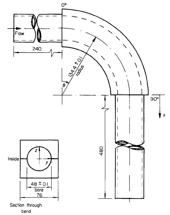
Figure 5.
Schematic of the experimental test 90° bend and coordinate system used by Enayet et al. [120] in their LDV flow measurements. Figure taken from Enayet et al. [120].
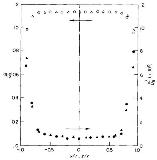
Figure 6.
Horizontal and vertical profiles for the mean velocity and turbulence intensity for turbulent flow at = 43,000 in the cross-sectional plane 0.58 diameters upstream of the bend inlet. Open circles and triangles correspond to horizontal and vertical velocity profile data, respectively, while filled circles and triangles refer to horizontal and vertical turbulence intensity profile data, respectively. Figure taken from Enayet et al. [120].
For the turbulent case ( = 43,000), Enayet et al. [120] found that the secondary flow that formed persisted six pipe diameters downstream of the bend outlet. Compared to the laminar flow at , the inlet boundary layers appear to be much thinner, and, as shown in Figure 6, the region of maximum velocity is characterized by a much larger central uniform plateau. This plays a significant role in the development of secondary flow downstream of the bend outlet.
LDV measurements of water flow at = 57,400 and 110,000 in a U-bend pipe were presented by Azzola et al. [121]. They provided profiles for the longitudinal and circumferential velocity components and for the longitudinal and circumferential turbulence intensity components at different stations within the U-bend and in the straight tangents upstream and downstream of the U-bend. As the flow enters the bend, the streamwise flow accelerates toward the outer wall and slows down in the central core, while a strong secondary flow develops during the first half of the U-bend. This cross-stream circumferential velocity pattern arises as a consequence of the transverse pressure gradient that sets in between the outer and inner bend walls. In the second half section of the U-bend, the cross-stream flow reverts its sense of motion and is directed toward the inner wall. Downstream of the U-bend outlet, the secondary flow gradually dissipates. Azzola et al.’s [121] compared their experimental results with additional numerical simulations for = 65,000, finding a reasonably good agreement between the experimental and numerical velocity profiles and circumferential turbulence intensity (see their Figures 2 and 3). However, Lee et al. [122] reported hot-wire measurements of the same flow parameters as Azzola et al. [121]. In particular, they were unable to reproduce the rms velocity fluctuation profiles reported by Azzola et al. [121], concluding that the profiles reported by these authors were erroneous.
Miniature hot-wire and wall-static pressure techniques were used by Anwer et al. [123] to investigate a fully developed turbulent flow at = 50,000 in a U-bend with . They measured the three components of the mean velocity and the six components of Reynolds stress along a horizontal and in a perpendicular plane in different pipe stations from 18 pipe diameters upstream to 18 pipe diameters downstream of the U-bend. Figure 7 shows a schematic drawing of the U-bend geometry along with the shape of the streamwise velocity profiles at selected stations and the form of the cross-stream (secondary) flow in the straight tangent downstream of the pipe bend. They found that a Dean-type secondary flow (i.e., two counter-rotating cell vortices) is established in the bend. However, the second cell disappears about one pipe diameter downstream of the U-bend exit, while complete flow recovery will take distances from the bend exit greater than 18 pipe diameters. In a follow-up investigation using the same experimental set-up of Anwer et al. [123], Anwer and So [124] used a variable interval time averaging technique to detect sublayer bursting in turbulent flow through a U-bend. They found that the measured circumferential wall shear stress distribution along with the spectral content of the wall shear signal and the associated bursting frequency confirm the previous finding that downstream of the bend return of the main flow to an unperturbed parabolic shape will take long distances.
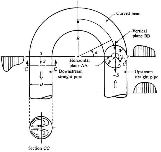
Figure 7.
Schematic drawing of the U-bend geometry used in Anwer et al.’s [123] and Anwer and So’s [124] experimental set up. Figure taken from Anwer and So [124].
4.2. Recent Experimental Studies
As was outlined by Kalpakli Vester et al. [14], the classical papers by Sudo et al. [125,126,127] are probably the most well cited and extensive experimental studies on the development of turbulent flow through and pipe bends. In particular, Sudo et al. [126] studied the steady turbulent flow in a circular bend with long upstream and downstream tangents. Using the innovative technique of rotating a probe with an inclined hot wire at = 60,000, they measured the three components of the mean and fluctuating velocities and Reynolds stresses at different pipe stations. In these experiments, a hot wire stem was mounted to a slip moving ring in the circumferential direction. In this method, the probe had to rotate several times at a prescribed point to obtain the velocity there. This technique is better suited than LDV to measure time-averaged and fluctuating velocity components in the three directions as well as their corresponding Reynolds stresses. This visualization of the velocity field was obtained by processing the signals from the hot wire probe in a computer, where they were transformed into mean and fluctuating velocities. The results indicate that as the primary flow enters the bend, it accelerates near the inner wall and soon forms a secondary flow, which in an angular section develops into a pair of vortices. At this stage, the Reynolds stresses are greater in the outer part of the cross-section. Toward the bend exit, the primary flow becomes greatly distorted, and both the turbulence intensity and the Reynolds stresses increase in the inner part of the bend cross-section. Downstream of the bend exit, the primary flow becomes progressively smoother, while the secondary flow weakens and the vortices break down. Later, Sudo et al. [125] performed similar experiments for turbulent flow in a square cross-section bend using a hot wire anemometer at = 40,000. In this case, the longitudinal and lateral components of the mean and fluctuating velocities were measured along with the turbulent intensity and components of the Reynolds stresses. As in the circular bend, after the flow enters the bend, it is accelerated near the inner bend wall and decelerated near the outer wall. At , a secondary flow of a vortex type arises, which gets stronger at larger angles. Toward the bend exit and about two pipe diameters downstream of the bend outlet (i.e., at in Sudo et al.’s notation), the primary flow looks quite distorted. Figure 8 shows contour plots of the longitudinal velocity component and secondary flow velocity vectors at different angular stations within the bend and along the downstream tangent. At and , a depression in the primary velocity contours is evident in the inner part of the bend cross-section. Owing to this large velocity gradient, the turbulence intensity and the Reynolds stresses increase around the velocity depression. As the main flow leaves the bend, the secondary flow attenuates beyond .
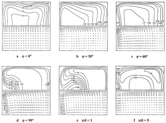
Figure 8.
Primary flow velocity contours (top panels) and secondary flow velocity vectors (bottom panels) for turbulent flow at = 40,000 (a–d) at different angular stations within a square-sectioned 90°-bend and (e,f) along the downstream tangent. Figure taken from Sudo et al. [125].
These experiments were also extended by Sudo et al. [127] to investigate the turbulent flow through a circular-sectioned U-bend. Longitudinal velocity contours through the bend and in the downstream section are shown in the left plot of Figure 9. Similarly to flow in a bend between and , the flow accelerates near the inner bend wall. At about , a secondary vortical flow forms as a result of the action of the strong pressure gradients between the outer and inner walls and the centrifugal force working on the fluid. Due to the transverse pressure gradients, the secondary flow still persists for and beyond the bend exit, although gradually weakening. In the downstream tangent, the flow returns slowly to its parabolic form, but it needs much longer distances than in the bend for full recovery. The distribution of the wall static pressure, defined as
is shown in the right plot of Figure 9. Here, is the pressure coefficient, is the pressure at in the straight pipe station upstream of the bend inlet and m s−1 is the bulk velocity, forming a flow with = 60,000.
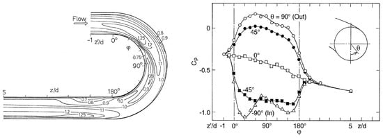
Figure 9.
(Left) Longitudinal velocity contours on the horizontal plane along a U-bend and its downstream tangent, normalized to the bulk velocity m s−1 for turbulent flow at = 60,000. (Right) Variation of the wall static pressure within the U-bend at different angles along the circular arc of the bend. Figures taken from Sudo et al. [127].
All previously discussed experimental investigations of laminar and turbulent pipe flow were performed under isothermal conditions. Under non-isothermal conditions, Wada et al. [128] constructed an experimental apparatus to study the convective heat transfer in the laminar pipe flow of highly viscous fluids ( Pa s) with and a temperature-dependent viscosity during cooling. The working viscous fluids consisted of solutions containing 80 wt% (with Pa s), 90 wt% (with Pa s) and 95 wt% (with Pa s) syrup. They performed an analysis of the pipe flow in terms of the dimensionless parameters and , where L is the pipe length, D is the pipe diameter, is the Péclet number and and are the fluid shear viscosities based on the inlet and wall temperatures, respectively. It was found that the thermal boundary layer is fully developed at , and, at this value, the maximum fluid velocity is observed to deviate significantly from Poiseuille flow. For , the deviations of the velocity profiles from Poiseuille flow are very small for the whole range of between 0.0005 and 0.05, while for close to zero, the velocity profile deviates from Poiseuille flow in the flow direction after heat transfer starts, and the deviation is seen to increase with increasing in the thermal entrance region. Based on numerically calculated Nusselt numbers (), a semi-empirical correlation was proposed to predict for highly viscous fluids (see Wada et al.’s [128] Equations (5)–(9)). In a more recent investigation, McNeil and Stuart [129] performed a series of experiments of highly viscous flow in pipeline components using a purpose-built test facility. For aqueous glycerin solutions with nominal viscosities between 1 and 550 mPa s, they obtained variations in the friction factor of the pipe as a function of , which fit very well the theoretical value for laminar flow in a circular cross-section pipe, . They also provided variations of the discharge coefficient for orifice plates and nozzles and loss coefficients for different systems, including a nozzle, an orifice plate, an abrupt enlargement and a globe valve for values between 10 and 200. They concluded that while existing methods appear to be quite adequate for prediction of friction factors and discharge coefficients for highly viscous flows, they are rather inaccurate for predicting loss coefficients.
Curvature-induced flow structures downstream of a bend exit at = 20,000 and 115,000 were investigated by Hellström et al. [130] using time-resolved stereoscopic particle image velocimetry (PIV). They performed snapshot proper orthogonal decomposition (POD) analysis of the flow at three different stations in the downstream tangent, finding that the most energetic flow structure does not conform with the usual Dean cell vortices, but, instead, it resembles a single-cell circulatory motion with an alternating direction of rotation, which they called the “swirl switching” mode. However, Dean vortices formed downstream of a circular bend were observed by Sakakibara and Machida [131] by synchronizing two sets of a PIV system.
Swirling turbulent flow in straight pipes was studied experimentally by a number of authors [132,133,134,135,136,137,138,139]. When a viscous fluid flows through a pipe rotating about its axis of symmetry, the tangential forces acting between the pipe wall and the fluid causes the latter to rotate with the pipe, giving rise to a flow pattern that differs from the one observed in conventional stationary pipes. Possibly, the first flow experiments in rotating straight tubes were carried out by White [132], who observed that in an axially rotating tube the laminar flow destabilizes, while the turbulent flow shows a clear tendency to stabilize. He also demonstrated that in a turbulent flow regime, the pressure losses decrease with an increasing rotation rate of the pipe. Flow velocity profiles in a rotating pipe were subsequently analyzed by Lavan et al. [133] for the case when a fully developed laminar flow is introduced into the pipe. Depending on the magnitude of the swirl number, defined as
where is the tangential velocity of the pipe wall, is the mean axial (or bulk) velocity and is the rotational Reynolds number, they observed a reverse flow in the wall region near the pipe inlet, which occurs for large values of S. The flow patterns and resistance in an axially rotating pipe were also investigated by Murakami and Kikuyama [134] for turbulent flow with and . Rotating pipes of lengths between and having a hydraulically smooth surface were used in the experiments. For rotating pipe lengths greater than , the hydraulic head loss was found to decrease for S increasing from 0.35 to 1.2. For , the suppression of the turbulence saturates and the head loss remains essentially unaltered. At pipe lengths , the velocity profiles were seen to become almost independent of the distance from the inlet. With a constant value of S, the axial velocity profile changes from turbulent to laminar. However, the ultimate shape of the axial velocity distribution was found to depend on the degree of turbulence suppression. These results were further confirmed by measurements with a three-hole pressure probe by Reich and Beer [136]. From measurements with hot-wire probes, Kikuyama et al. [135] confirmed previous findings obtained by White [132] that the pipe rotation destabilizes the flow in the inlet region due to a large shear induced by the rotating pipe wall and stabilizes the turbulent flow downstream due to the centrifugal force of the swirling velocity flow component.
Velocity measurements for water flow at = 20,000 through a 30 mm diameter pipe at a distance of from the inlet were performed by Imao et al. [137], using a single-component LDV operated in forward scatter. They observed that the turbulence intensity decreases gradually with increasing swirling S due to the increasing stabilizing effects of the centrifugal force. Measurements of the Reynolds shear stresses show that they experience a greater decrease compared to the turbulent kinetic energy, which results in the suppression of the momentum transfer by turbulent motion in the rotating pipe. Similar measurements by Rocklage-Marliani et al. [138] of turbulent flow in an axially rotating pipe at showed that the Reynolds shear stresses are reduced in the core flow region due to swirling, which, in addition, enhances the level of anisotropy in the fluctuating motion. In a relatively more recent work, Facciolo et al. [139] carried out LDV measurements of swirling turbulent flow in a rotating pipe and the initial development of a swirling jet, which arises when the turbulent swirling flow leaves the axially rotating pipe. The left graph of Figure 10 shows a schematic drawing of the swirling jet issuing from the rotating pipe. In agreement with previous observations by Murakami and Kikuyama [134], they found that within the rotating pipe, the cross-stream Reynolds stress impedes the flow to be in perfect solid body rotation. This appears to be true independently of how long is the rotating pipe. The measured streamwise velocity distribution was found to compare well with the scalings derived by Oberlack [140,141] for the azimuthal and axial mean fluid velocity components. A more complex flow situation involves the issuing swirling jet, whose core rotates in the opposite sense of the pipe relative to the laboratory reference frame. The right graph of Figure 10 shows the evolution of the mean axial velocity profile at three different positions downstream of the rotating pipe outlet with (no swirl) and (swirl). A more peaked profile is evident in the swirling flow case. At a short distance from the pipe exit (), the axial velocity of the jet is fairly unaffected, while further away from the pipe exit (at ), the jet velocity appears to be significantly larger for the case.
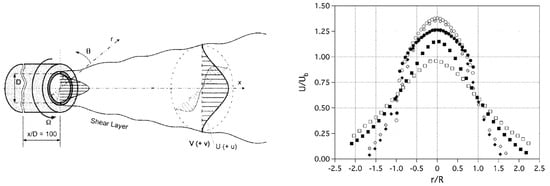
Figure 10.
(Left) Schematic drawing showing the development of a swirling jet as it leaves an axially rotating pipe. (Right) Measured mean axial velocity profiles showing the developing swirling jet at = 24,000 at varying streamwise positions from the rotating pipe outlet: (circles), (rhombuses), (squares) for (open symbols) and (filled symbols), where D is the rotating pipe diameter. Figures taken from Facciolo et al. [139].
Early experimental measurements of swirling flow in pipe bends were reported by Shimizu and Sugino [142], Anwer and So [143] and So and Anwer [144]. In particular, Shimizu and Sugino [142] investigated the flow patterns and the hydraulic losses in swirling flow through U-bends. They found that the swirling flow patterns in the U-bend are affected by the curvature and wall roughness of the bend, while the total energy losses depend on the strength of the swirl at the bend inlet, the bend curvature and the pipe wall roughness. Further experiments of swirling turbulent flow in a U-bend were performed by Anwer and So [143]. In their experiments, the rotating section was placed six pipe diameters upstream of the bend inlet for flow at = 50,000. They provided measurements of the wall static pressure, mean flow velocity components, Reynolds stresses and wall shear distribution around the pipe using pressure transducers, rotating-wires and surface hot-film gauges. The secondary flow pattern that forms consists of a single, off-center vortical cell that follows a wavy path along the bend. The measured wall static pressure was seen to be higher at the inner pipe bend contrary to what is expected in the case. This finding conforms with previous measurements by Kitoh [145] for flow through a curved pipe with large swirling. In addition, the wall shear was found to be the same at the inner and outer bend for . The superimposed pipe solid-body rotation leads to an increased turbulent production of the normal stresses near the pipe wall in both the radial and tangential directions. This, in turn, gives rise to more uniform and symmetric distributions of the normal stresses across the bend, which are then responsible for the generated insufficient vorticity to maintain a sustained secondary flow as in the case. In a follow-up paper, So and Anwer [144] investigated the flow recovery in the downstream tangent using the same experimental setup of Anwer and So [143], finding that full recovery of the mean flow occurs at approximately 74 pipe diameters downstream of the rotating section. They concluded that this recovery length is shorter than that observed in straight pipes, and, as a consequence, the effect of the bend curvature is to accelerate the swirl decay in the downstream section. Using a PIV method, Chang and Lee [146] investigated the swirling flow through a pipe bend of circular cross-section. They measured time-averaged velocity and turbulence intensity profiles with swirl and without swirl for 10,000 ≤ Re ≤ 25,000 at different stations within the bend and along the upstream and downstream tangents. Figure 11 shows the measured mean axial velocity profiles without swirl (the left column of plots) and with swirl (the right column of plots) at different values and pipe stations. In the non-swirl case, within the bend, the maximum velocity shifts toward the concave bend wall due to the influence of centrifugal forces. The shape of the velocity profiles remains unchanged even when is increased, consistently with previous findings. However, under pipe swirling conditions, the profiles look quite different, and again they remain almost the same regardless of the value. In contrast with the non-swirl case, the axial velocity in the upstream tangent and in the bend inlet is higher toward the concave bend wall. However, as a consequence of the tangential pipe wall velocity, the peak velocity within the bend and in the downstream tangent moves toward the convex bend wall.
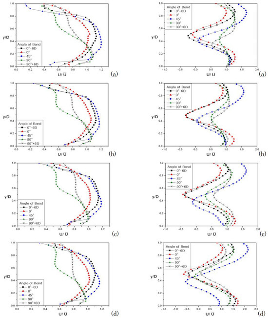
Figure 11.
Experimentally measured mean axial flow velocity with no-swirl (left column) and with swirl (right column) at different stations within a 90° circular bend and along the upstream and downstream tangents. In both columns, the flow is at (a) = 10,000, (b) 15,000, (c) 20,000 and (d) 25,000. Figures taken from Chang and Lee [146].
Experiments on flow downstream a pipe bend were later performed by Kalpakli and Örlü [147] using stereoscopic (TS) PIV for non-swirling and swirling flow conditions. The pipe facility consisted of a rotating straight upstream section connected to a still bend of curvature ratio and inner diameter mm. The flow medium consisted of air with = 14,000, 24,000 and 34,000. To acquire the three-dimensional flow field using TS-PIV, they used two high-speed C-MOS cameras, which were positioned at an angle of in backward–forward scattering. A laser light sheet of thickness mm was aligned at a distance 0.5 mm downstream of the bend exit, and raw images with a resolution of px were acquired from the measurements, which were then post-processed to obtain the velocity vectors. motion of the Dean vortices were additionally examined through snapshot proper orthogonal decomposition (POD), which is a powerful tool to ease visualization of the flow vorticity. They examined the turbulent flow structure at swirl numbers between and . The background color maps in the first column of Figure 12 shows the main velocity field scaled by the bulk velocity in a cross-sectional plane at downstream of the bend with a superimposed swirl from to , while the vectors visualize the secondary flow motion. The following three columns depict the zeroth, the first and the second POD spatial modes corresponding to each case. Mode zero represents the field averaged over time, while the other two modes represent the fluctuating part of the flow field. These plots illustrate the interplay between the swirling motion and the Dean vortical cells, as evidenced by the more energetic first and second POD modes.
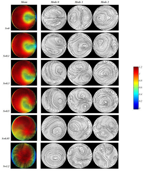
Figure 12.
Cross-stream mean velocity field at downstream of the bend exit for increasing swirl numbers from to (first column). The next three columns depict the zeroth, first and second POD modes, which are shown as cross-sectional streamlines to ease visualization of the secondary flow. The color-scale bar and numbers on the right border indicate the velocity contrast scaled by the bulk velocity. Figure taken from Kalplaki and Örlü [147].
Using the same experimental facility, Kalpakli Vester et al. [148] performed HWA and time-resolved stereoscopic PIV measurements of swirling turbulent flow at varying swirling intensities at a distance downstream of a bend outlet. In this case, a Platinum wire of nominal diameter 5 micron and length 1 mm soldered on straight prongs was used to perform the HWA measurements. A micro-manometer was used to calibrate the hot-wire ex situ. The hot-wires were operated in constant temperature anemometry mode at an overheat resistance ratio of 80%, while converged statistics was obtained by setting the sampling frequency to 20 kHz. They found that both experimental techniques produce results for the mean axial flow velocity that are in fairly good agreement. However, the single hot-wire method was found to provide a satisfactory estimate of the axial velocity when , while the agreement between the hot-wire and PIV data improves when , i.e., for the highest swirl intensity. Figure 13 illustrates the effect of the swirl number on the flow at = 24,000 downstream of the pipe bend from the PIV data. At , two bean-like shaped symmetrical Dean vortices form around the pipe horizontal axis. In this case, the two symmetrical cells persist even when is decreased to 14,000 or increased to 34,000. However, a slight increase in the swirl intensity to is enough to perturb the flow and break the symmetry of the Dean vortical cells. Since the upper vortex rotates in the same direction as the superimposed pipe wall rotation, it grows and dominates the flow as S is increased. In fact, at , the lower vortex has already disappeared. At higher swirl intensities the single vortex spans the whole pipe cross-section. At , the vortex is slightly off-center and is on the lower side of the wall of the pipe. Therefore, by gradually increasing the swirl number, a transition from a pair of vortices to a single vortex is observed.
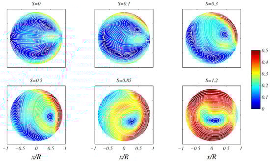
Figure 13.
Contour maps and sectional streamlines of the mean cross-stream flow velocity at a distance downstream of a 90° circular bend for = 24,000 and varying cross-stream swirl intensities between and . The color-scale bar and numbers on the right border indicate the cross-stream velocity contrast scaled by the bulk velocity. Figure taken from Kalpakli Vester et al. [148].
Laser-Doppler anemometry measurements of the no-swirl, secondary flow of water induced by a bend was also performed by Kim et al. [149]. Their experimental facility consists of upstream and downstream sections of acrylic pipes connected to a glass elbow. They tested three different flow conditions, corresponding to = 50,800 (their Run1), 101,600 (their Run2) and 203,200 (their Run3), and measured the mean axial flow velocity at distances of , and downstream of the bend exit. Figure 14 displays the measured axial velocity profiles in the downstream section. For the three values tried, the profiles are all coincident, implying that there exists a similarity in the flow structure at least for Reynolds numbers between 50,000 and 200,000. Sufficiently far from the bend exit, i.e., at , the flow looks parabolic. However, at = 203,200, the velocity profile appears to be slightly flatter compared to Run1 and Run2 working at lower values. Kim et al. [149] pointed out that this feature is consistent with previous experimental measurements of turbulent pipe flow by Zaragola and Smits [150]. Wang et al. [151] performed additional experiments on the flow of water through a elbow at = 44,805.
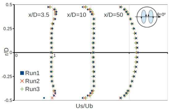
Figure 14.
Measured axial velocity profiles at three different stations downstream of a 90° bend for turbulent flow at = 50,800 (Run1), 101,600 (Run2) and 203,200 (Run3). Figure taken from Kim et al. [149] (Characteristics of secondary flow induced by 90-degree elbow in turbulent pipe flow, Kim, J.; Yadav, M.; Kim, S., Engineering Applications of Computational Fluid Mechanics, copyright © Department of Civil & Environmenal Engineering, The Hong Kong Polytechnic University, reprinted by permission of Informa UK Limited, trading Taylor & Francis Group, https://www.tandfonline.com (accessed on 16 February 2025) on behalf of Department of Civil & Environmental Engineering, The Hong Kong Polytechnic University).
Recently, Synowiec et al. [152] provided measurements of velocities and flow rates downstream of a bend using an ultrasonic flowmeter with clamp-on sensors for water flow at = 70,000 and 100,000. Axial velocity profiles and cross-stream velocity fields were measured at the exit plane of the bend and downstream of the bend at every 1 pipe diameter until 15 diameters are reached. They found that at a distance from the bend exit, it is possible to perform correct measurements with errors less than 2% of the flow stream value. At distances , the errors drop to about 1.3%. However, in all downstream stations, the level of error is larger for the = 100,000 flow. On the other hand, it is well known that curved pipes may represent a device for enhanced heat transfer with the outside because the emerging secondary flow can promote mixing in the main flow and break the thermal boundary layer. In particular, Guo et al. [153] performed recent experiments to investigate turbulent flow and heat transfer through a straight pipe and a pipe bend. A hot-air generator was used to produce high-temperature airflow. The streamwise velocity and temperature field on the pipe wall were measured using hot-wire anemometers and thermal couples, respectively. At the pipe inlet, the airflow is set to 402 K with a bulk velocity corresponding to 60,000. For flow in a straight pipe, they found that the cross-sectional mean temperature decreases monotonically in the streamwise direction, while in a sharp bend, the temperature first increases and then decreases to increase again.
In a very recent paper, Atashi et al. [154] conducted an experimental investigation of the scour geometry downstream of a W-Weir in a bent channel. In particular, they measured the flow pattern and shear stress changes in different discharges and positions along the inner and outer bends. Figure 15 shows a schematic view of their laboratory flume and test bend. The W-Weir (in red) was constructed using a 1 mm thick galvanized sheet and was installed at angles , and within the bend. They considered two Froude numbers, and 0.28, where
with v being the main flow velocity, g the acceleration of gravity and L a characteristic length scale. The experimental results showed that there was a lower depth of scour and a lower volume of sediment removal when the weir was placed at the bend exit (see Figure 16, where a topography of the bend is displayed for at three installation angles). These results corroborated previous findings by Bhuiyan et al. [155], who observed that the best place to install the W-Weir was just immediately downstream of the bend, where the flow pattern exhibits severe turbulence. Furthermore, compared to installation of the W-Weir at and , erosion on the outer bend wall was reduced by 39% and 37%, respectively, when the W-Weir was placed at .
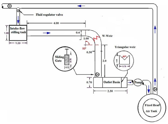
Figure 15.
Schematic view of the laboratory flume and test bend used by Atashi et al. [154] for their measurements of the flow pattern and erosion in a sharp bend around a W-Weir. All numbers express dimensions in meters. The arrows indicate the flow direction. Figure taken from Atashi et al. [154].
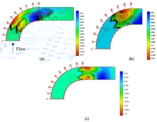
Figure 16.
Contour maps of the scour depth for and W-Weir installation at (a) 30°, (b) and (c) 90° within the test bend. All numbers on the outer bend side are in meters. Figure taken from Atashi et al. [154].
The investigation of pulsatile flow through an S-shaped double-bend pipe in conditions resembling an automotive engine environment is of great interest to improve the conversion efficiency and durability of close-coupled catalytic converters (CCCs). In general, the structure of the exhaust gas flow is rather complex because of its turbulent nature and the manifold geometry of the CCC. The high conversion efficiency and durability of the CCC will require a uniform flow in front of or behind it. Experiments addressed to investigate the effect of the mass flow rate and pulsation frequency on the velocity profiles were conducted by Liu et al. [156] by means of HWA, while Persoons et al. [157] measured the velocity distribution in the presence of reverse flow in a real CCC. In a more recent work, Oki et al. [158] performed PIV measurements of streamwise and secondary flow velocities in an S-shaped square section exhaust pipe. A pulsatile flow is built up at the inlet plane of the pipe. On the left side of Figure 17 is shown a drawing of the S-shaped exhaust pipe, while the velocity fields as obtained from two-dimensional two-component PIV measurements in the planes of the first and second bend are shown on the right side. Across the first bend, the flow velocity is higher near the inner wall. As the flow leaves the first bend, the zone of higher flow velocity enters the second bend near its outer side wall. The shift of the high-speed region from inner wall in the first bend to outer wall in the second bend is due to the secondary flow arising by the effects of centrifugal forces. Cross-stream velocity maps were measured downstream of the second bend exit, showing the formation of a pair of counter-rotating symmetric vortices over a wide area of the cross-section (see Oki et al.’s [158] Figure 10).
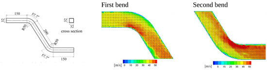
Figure 17.
(Left) Schematic drawing of the S-shaped exhaust pipe. All lengths shown are in mm. (Right) Measured velocity field and vectors in the central planes of the first and second bends. Figures taken from Oki et al. [158].
Heat transfer characteristics of pipes with single bends [153] and coil-type piping (see Ref. [15] and references therein) have been actively investigated because of applications to heat exchangers. However, studies of heat transfer in turbulent flow through an S-shaped pipe are much less abundant. An evaluation of heat dissipation and the Nusselt number () has only been recently provided by Kato et al. [159]. They used PIV techniques to measure the mean velocity and turbulent kinetic energy of hot airflow through a double bend of square section at = 60,000. The air was injected at the pipe entry with an approximate temperature of 399 K and a pressure of 118 kPa. They compared the heat transfer characteristics for the S-shaped pipe with those for a simple straight pipe. The left graph of Figure 18 shows a schematic of the double bend and straight test sections with marks of the positions where K-type thermal couples were placed to provide measurements of the circumferential temperature. As shown on the right of Figure 18, near the pipe entrance, the temperature is higher at the cental core. For a straight pipe, the core temperature decreases progressively as the flow moves downstream. In the S-shaped pipe, the core temperature shifts from the center to the outer wall side at the exit of the first bend. As suggested by Guo et al. [153], the shift is caused by the compressive heating of the fluid on the outer side of the bend due to centrifugal forces. As the flow leaves the first bend, the region of higher flow temperature remains attached to the outer pipe wall, and a strong temperature gradient is established through the whole pipe cross-section. As the flow enters the second bend, the temperature decreases because of much lower eddy diffusion there, and, as a result, the flow near the outer pipe wall at the exit of the second bend cools down.
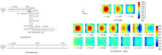
Figure 18.
(Left) Schematic view of (a) the S-shaped and (b) straight pipe used in the experiments of Kato et al. [159]. The stations where thermal couples were placed to measure the circumferential temperature are marked. (Right) Maps of the circumferential temperature through the measuring stations along (a) the straight and (b) the S-shaped pipe. Figures taken from Kato et al. [159].
Another interesting application of these studies is the efficiency of irrigation water utilization. This is particularly true because the water distribution outlets in irrigation zones are predominantly right-angled; therefore, progressive erosion, sedimentation and structural damage of the irrigation system is a main concern. Recently, Shen et al. [160] have performed indoor physical model experiments to examine the distribution of channel flow velocity, pipeline flow rate, variations in water surface profiles, diversion ratio, circulation intensity and turbulence energy at different water depths.
5. Numerical Modeling: Flow of Newtonian Fluids in Pipes
Models of fluid flow in pipes and ducts, relying on numerical solutions of the Navier–Stokes equations, started to appear in the early 1970s. Due to their complex and resource-demanding character, they have grown in number in parallel with the advent of increasing computing facilities. However, in the early 1960s, Bodoia and Osterle [161] and Collins and Schowalter [162] reported numerical steady-state solutions for the laminar flow of an incompressible fluid in the entrance region of a straight channel using a marching finite-difference (FD) technique. Similar calculations for a straight circular pipe were presented shortly after by Hornbeck [163]. Model simulations can be divided into two main categories, depending on whether they have been performed using conventional mesh-dependent methods or particle-based techniques. Here, we shall only review models of Newtonian fluid flow in straight and bent pipes and leave the flow of non-Newtonian fluids in Section 6. As was outlined by Kalpakli Vester et al. [14], numerical simulations of turbulent flow have been largely based on Reynolds-averaged Navier-Stokes (RANS) models even though they may not lead to good predictions owing to the anisotropy of the turbulent motion. For flow in bent pipes, flow separation and the secondary flow imposed by the bend curvature are additional important factors. However, Wallin and Johansson [164] have shown that under anisotropic turbulence and curved streamlines, Reynolds stress models (RSMs) perform better than eddy viscosity models (EVMs), although the former could also fail for small curvature ratios (i.e., sharp bends) [165].
5.1. Pipe Flow Modeling with Mesh-Dependent Methods
The flow through pipe bends is considerably more complex and resource-demanding than the flow through straight pipes. This explains why most numerical work since 1970 has focused more on studying the flow in curved pipes. The interested reader can refer to Berger et al. [20] for an overview of earlier theoretical work on fluid flow in pipe bends. The discussion of results using mesh-dependent methods can be subdivided into four main groups: (1) transitional and turbulent flows in straight and bent pipes, (2) secondary flow in bent pipes, (3) pipe swirling flows and (4) pulsatile flows.
5.1.1. Turbulent Flow Modeling
A first attempt to reproduce numerically available experimental data on the total pressure and yaw relative to the pipe axis for flow in U- and S-bends was reported by Rowe [166], who assumed an inviscid fluid to reduce the problem to solve a Poisson-like equation for the stream function using a Gauss–Seidel relaxation method. Five years later, in 1975, Pantakar et al. [167] performed what appear to be the first numerical simulations to predict turbulent flow in curved pipes. They used FD methods to solve the Navier–Stokes equations in three-space dimensions coupled to the turbulence model. Despite the rather coarse spatial resolution used, their simulations reproduced fairly well the axial velocity profiles obtained experimentally by Mori and Nakayama [168] for fully developed turbulent flow. Azzola et al. [121] presented simulations of laminar and turbulent flow in a U-bend using finite volume methods (FVMs) coupled to the standard effective viscosity model to approximate the turbulent stress field. They found reasonably good agreement with their own measurements of the longitudinal and circumferential velocity components within the bend (see their Figures 3 and 4), including the secondary flow reversals. Based on FVM coupled to the model, Al-Rafai et al. [169] studied turbulent flow at = 34,132 through bends with and 0.14. They found that the secondary flow is stronger in the bend. However, they did not obtain good agreement with their own LDV measurements of the axial velocity profiles, which can be attributed largely to the coarse resolution used in their simulations. The turbulent flow through a single bend and a double bend out-of-plane both of circular section was later on investigated numerically by Hilgenstock and Ernst [170] with the aid of the commercial computer package Fluent v4.3 based on FVM discretization of the Navier–Stokes equations. They compared the performance of the turbulence model with that of the Renormalization group (RNG) model. For both types of bends, the RNG turbulence model was found to match better the experimental axial velocity profiles provided by the German National Metrology Institute.
The first numerical simulations of a fully developed turbulent flow in a curved pipe with the aid of Large-Eddy Simulation (LES) were reported by Boersma and Nieuwstadt [171,172] for the case of an infinitely long curved pipe using periodic boundary conditions. They employed a FVM discretization of the Navier–Stokes equations written in toroidal coordinates. Consistently with observations of flow in a curved channel, they found that the turbulence intensities are much larger near the outer wall of the bend than near the inner wall, and, in contrast to flow in a straight pipe, the Reynolds stresses are larger in the core region of the pipe. Along with Boersma and Nieuwstadt’s [172] work, one of the first Direct Numerical Simulations (DNSs) was presented in 1999 by Moser et al. [173], who considered fully developed flow in a channel at low Reynolds numbers (i.e., , 300 and 590). The numerical simulations were made with the aid of a variant of the Kim et al.’s [174] code, relying on a Chebyshev-tau formulation in the wall-normal direction and a Fourier representation in the horizontal directions. A few years later, Quadrio and Luchini [175] performed for the first time DNS to investigate the turbulent flow in a pipe with annular cross-section by solving the Navier–Stokes equations using Fourier spectral techniques. The results in terms of mean flow properties and main turbulence statistics indicate that in an annular pipe with relatively low transverse curvature (i.e., and 1), the flow deviates from a planar flow contrary to previous beliefs.
Sugiyama and Hitomi [176] simulated turbulent flow through a pipe bend of circular cross-section using an algebraic RSM and FD methods for discretization of the governing equations. They found that their numerical scheme can predict the developing behavior of the secondary flow in good agreement with experimental results. Although the Reynolds stresses in the bend are qualitatively well predicted by the simulations, their values are quantitatively underpredicted. On the other hand, Rütten et al. [177] investigated the turbulent flow through a pipe bend at values in the range between 5000 and 27,000 using a LES approach with the aid of the advection upstream splitting FD method [178]. They found that as a result of a shear layer instability, the spectra of the forces exerted by the fluid on the pipe wall exhibit for all values considered a peak at Strouhal numbers between 0.2 and 0.3, where the Strouhal number is defined as
where is the frequency of the vortex shedding in Hertz, L is a typical length of the system and v is the flow velocity. At = 27,000, the force spectra also peak at . The analysis revealed that the low-frequency oscillations that are perceptible throughout the pipe wall are due to the Dean vortices, which alternate in strength and between clockwise and counterclockwise rotation in the downstream tangent, similarly to the switch-swirling flow pattern phenomenon detected by Tunstall and Harvey [111] in flow experiments at miter bends. With the aid of the software package Fluent v6.2, Rup et al. [179] solved the RANS equations using the RSM turbulence model to simulate the volumetric flow rate through a square-sectioned duct bend. A comparison with the experimental axial velocity profiles obtained by Sudo et al. [125] shows that there is good agreement between the experimental and numerical profiles within the bend, while at 10 hydraulic diameters downstream of the bend exit, the front axial velocity is underpredicted by the numerical simulation. FVM simulations of turbulent flow in a pipe elbow at relatively high values of between 50,800 and 203,200 were reported by Kim et al. [149] with the aid of the commercial software OpenFOAM 2.1. The numerical axial velocity profiles at three different pipe stations were found to reproduce very well their own LDV measurements displayed in Figure 14.
Pellegrini et al. [180] performed a comparative study of different turbulence models and wall treatment for pipe flow in a bend at transitional Reynolds number. In particular, they solved the RANS equations with the aid of the commercial CFD code Star-CCM+ 5.02.009 using as closures the and eddy viscosity models and the Reynolds Stress Transport (RST) model. For the closure, the flow close to the pipe wall was solved using a low-Re and a two layer formulation, while the closure was tested only with a low-Re wall treatment and the RST model with a two layer formulation. As shown in Figure 19, the axial velocity profiles at downstream of the bend exit for the different models are compared with PIV experimental results [181] and LES data [177]. Although the closure with the two-layer formulation for the wall treatment underestimates the profile of the fully developed flow, it is able to capture the main characteristics of the flow in the downstream tangent. DNS simulations with the aid of the ANSYS-CFX11 code to examine the turbulence flow structure were performed by Di Liberto et al. [182]. Three different curvature ratios (straight pipe; = 17,000) and and 0.3 at = 15,000 and 12,000, respectively, were considered. The results of the simulations indicate that the level of turbulence decreases with the curvature, and, in general, it is lower in a curved pipe than in a straight one. However, it was realized that in curved pipes, convection plays a significant role in the turbulence budget, especially within the Dean vortices.
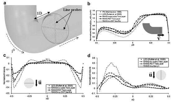
Figure 19.
Comparison of velocity profiles downstream of a 90° pipe bend as obtained from CFD simulations with different closure models and wall treatment formulations. (a) Pipe bend showing the location of the line probes. The dashed arrows indicate the flow direction, (b) axial velocity on the vertical symmetry plane, (c) radial velocity on the horizontal symmetry plane and (d) radial velocity on the vertical symmetry plane. The numerical profiles are compared with the experimental data of Meinke et al. [181] and the LES calculations of Rütten et al. [177]. Figure taken from Pellegrini et al. [180].
Noorani et al. [183] performed DNS based on spectral element methods (SEMs) to investigate fully developed, statistically steady turbulent flow in straight and bent pipes at moderate values between 5300 and 11,700. An overview of the simulated flow is given in Figure 20, where the instantaneous axial velocity is displayed for = 11,700 and three pipe configurations with (straight pipe), (mildly curved pipe) and (highly curved pipe). As the curvature ratio increases, the flow loses its azimuthal homogeneity as the increasing centrifugal forces deflect the flow from the center to the outer wall. Further DNS based on SEM for the study of turbulent pipe flow at moderately values was presented by El Khoury et al. [184]. They put in perspective their results with other simulation data sets, finding that the pressure is the flow variable that differs the most between pipes, channels and boundary layers since significant differences in the mean and pressure fluctuations were observed. More recently, Wang et al. [185] performed DNS based on a high-order SEM to study the unsteady oscillations of the Dean vortices formed in turbulent flow in a bend of curvature ratio at . Time series and power spectral density analysis of the velocity fluctuations along the pipe axis of symmetry demonstrated that multiple dominant frequencies exist in the flow, which may vary depending on the flow region. Measurements of the lateral wall pressure force show that the force oscillations are amplified within the bend, with their maximum values occurring at downstream of the bend exit. A strong correlation was also observed between the mass flow rate and the horizontal force oscillations. Highly resolved DNS based on SEM was recently presented by Yao et al. [186] to examine turbulence statistics in a smooth straight circular pipe at . In contrast with DNS results for turbulent channel flow at [187], the mean velocity has not yet developed a logarithmic region at this value. However, similar to observations in the channel, the one-dimensional spectrum of the axial velocity shows a dependence at intermediate distance from the wall, where k denotes the wavenumber. A modified RNG model was used by Liu et al. [188] to study blood flow in a U-bend with strong curvature. The numerically predicted distribution of the pressure coefficient on the medial and lateral walls was found to agree well with available experimental data (see Liu et al.’s [188] Figures 5 and 6).
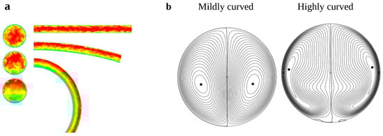
Figure 20.
(a) Maps of the streamwise velocity normalized by the bulk velocity at pipe cross-sections (left) and equatorial mid-plane (right) for = 11,700. Straight (), mildly curved () and highly curved () pipes are displayed. The colors indicate the velocity contrast and range from 0 (blue, low) to 1.25 (red, high) in normalized units. (b) Iso-contours of the stream function for flow at = 11,700 in the mildly () and highly () curved pipes. The filled dots mark the center of counter-rotating Dean vortices. Figure taken from Noorani et al. [183].
Interesting results from turbulent pipe flow simulations using LES combined with a characteristic-based split scheme for the discretization of the Navier–Stokes equations were presented later on by Tan et al. [189]. For a circular-sectioned bend, they observed for the first time a four-vortex structure within the bend. A year later, studies using LES to investigate turbulent flow in pipe bends were reported in Refs. [165,190,191]. For instance, Röhrig et al. [165] performed a comparative study between LES and RANS models of turbulent flow in a pipe bend at = 14,000 and 34,000. They confirmed the expectation that LES provides superior results compared to the RANS approach but at the cost of a much higher computational burden. The results of the simulations show that LES can accurately predict the mean velocity field across the pipe elbow and the occurrence of secondary vortices. Heat transfer in turbulent curved-pipe flow was further investigated by Kang and Yang [191] using a LES approach. At and curvature ratios of 0.01, 0.05 and 0.1, they found that, apart from the emergence of a pair of counter-rotating vortices, the mean friction factor and the Nusselt number increase with increasing curvature, indicating an enhancement of heat transfer at the expense of increased friction. In this way, the local heat transfer on the outer wall is enhanced by the pipe curvature, while the mean and fluctuating axial velocity components are strongly correlated with the temperature.
The swirl switching phenomenon—the large-scale oscillations that occur in the flow downstream of the bend—has been further studied by Carlsson et al. [192] for flow at = 34,000 in pipe bends with different curvature ratios (, 0.5, 0.7 and 1). In this case, the Navier–Stokes equations were solved implicitly using a pressure implicit split operator algorithm. Since the phenomenon can be classified into a high-frequency and a low-frequency switching, Carlsson et al. [192] proposed that the high-frequency switching originates from flow structures formed in the bend and increases in importance for sharp curvatures, while the low-frequency switching arises from large-scale motions produced in the upstream pipe flow. Using DNS, Schlatter et al. [193] analyzed for the first time by means of three-dimensional POD the spatial and temporal contributions of the flow oscillations responsible for the swirl switching phenomenon. For flow simulations with two bends of curvature ratios and 0.3, they inferred that the swirl switching originates from a single low-frequency, three-dimensional POD mode, and, in contrast to Carlsson et al. [192], they showed that the upstream turbulent flow has no relation with the origin of the swirl switching phenomenon.
The turbulent flow at = 11,500 through a square-sectioned L-shaped pipe was recently simulated by Venters et al. [194] using DNS. The results were compared to equivalent RANS data and experimental measurements [195]. Figure 21a–c show mean velocity maps at the midplane for the simulations and the experiment. As a consequence of the elbow geometry, the incoming flow is deflected to the outer side wall, and a recirculation flow is created near the inner wall, which occupies about 20% of the pipe width. The recirculation flow is clearly visible at . Further downstream, the flow structure predicted by the RANS model differs from the DNS and the experiment. Although both numerical schemes predict the experimental mean velocity profiles in the upstream section fairly well, the RANS simulation fails to accurately reproduce the flow characteristics in the downstream section, while the DNS closely matches the experimental data with a maximum difference of only 2% as shown in Figure 21d–f.
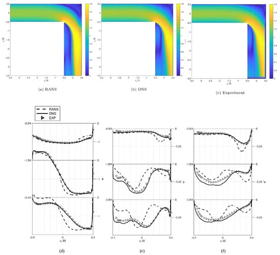
Figure 21.
Intensity maps of the mean velocity field through a square-sectioned L-shape pipe bend: (a) RANS calculation, (b) DNS and (c) experiment. The bottom panel shows (d) the streamwise velocity, (e) the streamwise turbulence intensity and (f) the wall-normal turbulence intensity profiles at three downstream locations. Figures taken from Venters et al. [194].
Most recent numerical simulations aimed at studying turbulent flow characteristics in pipes have focused on flow in a bend [196,197,198] because it is one of the most frequently used fittings in practice. For example, Fazeli et al. [197] conducted simulations of flow in a bend with the aid of the CFD toolbox OpenFOAM coupled to a wall-modeled LES closure. On par with standard LES and RSM, these authors showed that wall-modeled LES can correctly predict the overall shape of experimental streamwise velocity profiles in a pipe bend. OpenFOAM-based simulations with a standard LES turbulence model were presented by Mikuž et al. [198] to investigate how far the flow asymmetry induced by a bend extends downstream. Their results indicate that, at , from 10 to 40 pipe diameters downstream of the bend are required for the flow to become nearly symmetric, while, at = 10,000, this length ranges from 10 to 30 pipe diameters. The flow asymmetry was observed to be so persistent that even 100 pipe diameters may not suffice to full recovery of the laminar flow. On the other hand, Smyk et al. [196] reported highly resolved simulations of flow in a bend using ANSYS Fluent and a turbulence model with the aim to investigate pressure losses for flow at 100,000. For , the Darcy friction factor is fairly well reproduced by the simulations, while for 20,000 a minor loss coefficient of about 0.2 was predicted, which is close to the engineering value of 0.22. Also, the flow dead zone behind the bend was found to be smaller at higher . Visualization of the secondary flow induced by the bend curvature was improved using the Q-criterion for vortex identification [199]. Figure 22 shows a detailed view of the vortices at and 100,000 on the exit plane of the elbow.
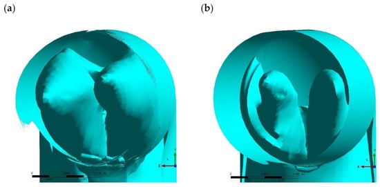
Figure 22.
Q iso surfaces for level 0.005 showing how much the vortices contribute to the flow in the elbow at different . The views display the vortical structure on the exit plane of a 90° bend of circular cross-section at (a) and (b) = 100,000. Figures taken from Smyk et al. [196].
The effects of varying the bending angle on pipe flow in a circular-sectioned bend were studied by Zhang et al. [200] by solving the RANS equations with the aid of the ANSYS Fluent software. A realizable turbulence model was used to solve the flow characteristics at = 14,000. Figure 23 shows maps of the pressure and streamwise velocity distributions for different bend angles. Variation of the bend angle affects the wake flow in the downstream tangent. The greater the bend angle, the greater the distance needed to reestablish laminar flow. It was also found that, as the bend sharpness increases, the global pressure losses show an increase–decrease–increase trending, while centrifugal forces affect the flow most for pipe bends close to . This explains why the secondary flow is stronger in a bend, as illustrated in Figure 24, which shows cross-stream velocity maps in pipe bends with different angles at different stations downstream of the elbow. Recently, Jia et al. [201] performed a numerical simulation analysis of flow in a circular-sectioned S-shaped pipe with short turning sections and no extended straight pipe segments. Their analysis predicted the most stable flow region for the optimal placement of a thermal mass flow velocity meter, thereby providing a new methodology and practical basis for flow measurement in complex pipeline systems. Previous simulations of pulsatile flow in an S-shaped exhaust pipe of square cross-section aimed at reproducing experimentally obtained data (see Figure 17) were presented by Oki et al. [158].
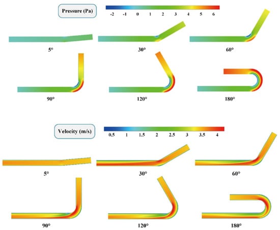
Figure 23.
Intensity maps showing the pressure and streamwise velocity fields in pipes of circular cross-section with different bend angles. Figure taken from Zhang et al. [200].
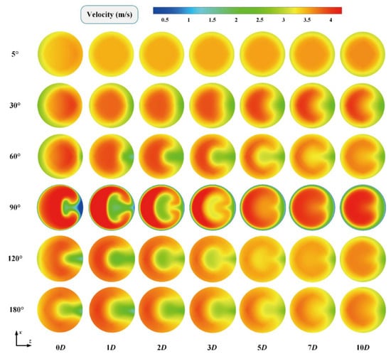
Figure 24.
Cross-stream velocity maps in pipes of circular cross-section with different bend angles at different stations downstream of the elbow for the simulations of Figure 23. Figure taken from Zhang et al. [200].
Turbulent flow in closed ducts and pipes has been studied by numerical simulations more intensively than in channels, probably because in the latter case, the free surface complicates the flow configuration a bit more. However, in the last ten years, several studies have focused on simulating this type of flow [202,203,204,205,206,207,208]. A characteristic feature of channel flows compared to wall-bounded flows is the occurrence of Prandtl secondary flows of the second kind [209,210] and the presence of a velocity dip, i.e., a peak velocity that occurs at some depth below the free surface. Recently, Yu et al. [207] performed DNS of turbulent flow in an open channel for in the range 106,000 and various duct aspect ratios, using their own numerical solver STREAmS [211,212]. They found that the depth of the peak velocity increases with increasing , yielding a more symmetric flow with respect to the horizontal midplane. Further DNS of pressure-driven turbulent channel flow was performed by Liakopoulos and Palasis [208] for 10,000. In particular, the skin friction coefficient obtained from their simulations showed excellent agreement with Dean’s formula based on experimental measurements of high flows in open channels with aspect ratios of the ducts greater than 1:12 [213].
Numerical simulations of other pipe flow configurations have also been reported in the literature. For example, Zambrano et al. [214] performed three-dimensional simulations of oil flow in a circular-sectioned pipe with a diffuser, using the commercial code Fluent 6.3. They compared the flow results for three different turbulence closures, namely, the standard , the Realizable and the RNG-based model. The Standard Wall Functions (SWFs) and the Enhanced Wall Treatment (EWT) approaches were implemented to describe the near-wall flow. They concluded that the RNG model provided the best comparison to the experimental data and the best prediction concerning the reattachment length particularly when working with the EWT method. The RANS equations coupled to the standard turbulence closure were solved by Morad et al. [215] using the commercial software Fluent 16.1 and COMSOL Multiphysics 5.4 to investigate the flow structure through a vertical pipe at low to moderate Reynolds numbers. On the other hand, the effects of surface roughness on Stokes flow in a straight pipe of circular cross-section were analyzed theoretically and numerically by Song et al. [216]. In particular, they studied the effects of periodically structured surface roughness on the flow field and the pressure losses for flow at low . These authors found that under the presence of periodic surface roughness, the flow fluctuates periodically and the pressure drop grows. Moreover, the pressure drop increases as a result of increasing the relative roughness. Altowayti et al. [217] presented what they called a smart mathematical model to predict water flow and losses through leak openings in pipeline systems. The solution method relies on an iterative method that leads to the measurement of the minor and major losses of water and was demonstrated to work on the side of improving the capability to monitor water supply management daily, which is one of the most important operational challenges for domestic water supply companies. In order to speed up the calculation of laminar flow of liquids through pipes, Wiens [218] has recently proposed to use three-dimensional CFD simulations to derive appropriate correction factors that can work for existing one-dimensional solution methods to predict the characteristics of laminar flow under small pressure changes.
Recently, numerical simulations applied to solving real-life problems involving the flow through pipeline systems have started to appear. For example, Wu et al. [219] have performed simulations of airflow through a rectangular elbow in order to improve indoor air quality from a uniform push–pull ventilation device. The flow downstream of a flow conditioner with a bundle of tubes was also studied numerically by Yin et al. [220], which is a pipe configuration widely used by the offshore and subsea oil and gas industry to improve the precision of flow rate measurements in pipeline systems. Numerical simulations applied to turbulent flow in submarine pipe bends and blind-tee pipelines have also been reported by Yang et al. [221] and Han et al. [222], respectively. For instance, blind tees are pipe junctions that are widely used to improve mixing flow conditions in offshore oil and gas transportation. Due to the flow circulation and backflow in the blind-tee pipe, this type of flow exhibits a high complexity. As an illustration of this, Figure 25 shows the streamlines describing the flow structure in a blind-tee pipe as calculated by Han et al. [222] using the commercial software ANSYS CFX 14.5 to solve the unsteady RANS equations. A similarly complex flow is the turbulent one developing in a confluent channel [223].
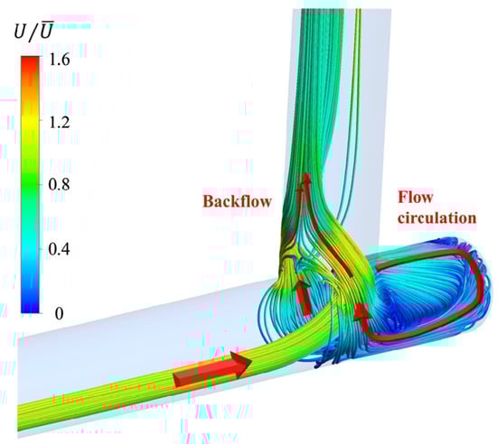
Figure 25.
Streamlines showing the three-dimensional circulation and backflow in a blind-tee pipe of length twice the circular pipe diameter as calculated with ANSYS CFX. The red arrows indicate the main flow direction. Figure taken from Han et al. [222].
Modern numerical simulations of turbulent pipe flow are generally based on LES approaches or DNS. Since DNS resolves all the scales of turbulence directly by solving the Navier–Stokes equations without the use of any modeling approximations, it is theoretically highly accurate at the expense of requiring immense computational resources. It is, therefore, feasible only for flows with relatively low Re and small domains. LES, on the other hand, resolves the larger scales of turbulence explicitly while modeling the smaller scales that are more universal in nature using subgrid-scale models. By filtering the flow field, LES reduces the computational cost compared to DNS while still capturing the essential features of turbulence. This makes LES a powerful tool for studying flows with complex geometries and high Re that are beyond the reach of DNS. LES also offers better accuracy than traditional RANS models, which, being best suited for steady flows, oversimplify the turbulent flow structures under unsteady conditions.
5.1.2. Secondary Flow Modeling
Turbulence-driven secondary flow in the form of streamwise vorticity in bent pipes is a natural consequence of the pipe curvature. Although in the previous section this aspect was touched upon several times when reviewing the main results of numerical studies of turbulent flow in curved pipes, here we shall focus only on numerical work dealing with prediction of embedded-vortex flows with a focus on their type and structure. It is well known that secondary flows can be classified into two types, namely, the Prandtl secondary flow of the first kind, which in bent pipes arises as a strong in-plane secondary flow driven by the centrifugal force and the pressure gradient across the pipe cross-section, and the Prandtl secondary flow of the second kind, which is generated via the spatial heterogeneity of Reynolds stresses. For early numerical work on turbulent secondary flows, the interested reader is referred to the review paper by Bradshaw [209] and references therein. Chin et al. [224] have presented a recent study on backflow events under the effects of the Prandtl secondary flow of the first kind. Nikitin et al. [210] give a complete description of the physical mechanisms behind the emergence of Prandtl secondary flows of the second kind in open channels and channels with inhomogeneous rough walls. In straight pipes, secondary flows of the second kind occur only under turbulent conditions, while those of the first kind can appear in curved pipes for laminar and turbulent flows under the action of centrifugal effects. Another difference is that the intensity of secondary flows of the first kind can be tens of percent of the main stream velocity. In contrast, the secondary flows of the second kind are significantly less intense, and usually they are not greater than about 3% of the main stream velocity. On the other hand, Salesky et al. [225] have demonstrated that another type of turbulent secondary flow can arise as a result of spanwise variability in the surface heat flux in unstable turbulent channels, which they defined as Prandtl secondary flows of the third kind.
Lai et al. [226] investigated the generation of secondary flow in a U-bend at = 50,000 and using a RSM approach. They found that the secondary flow pattern consisted of three pairs of vortices that formed within the bend. The primary vortex pair consisted of the usual Dean cell that forms in pipe bends as a result of the imbalance between the centrifugal forces and the radial perssure gradient. The second pair of vortices is a pressure-driven cross-stream flow reversal near the pipe center. This second cell formed approximately halfway along the U-bend () and dissipated shortly thereafter at . The third vortex pair was identified as a turbulence-driven circulatory motion formed near the outer bend wall at approximately . This vortex pair was seen to completely dissipate after 7 pipe diameters downstream of the bend, while full laminar flow is recovered after only 42 pipe diameters. However, as stressed by Kalpakli Vester et al. [14], there is still no theoretical or experimental evidence to date confirming the existence of a third cell in turbulent flow through pipe bends. Fjällman et al. [227] used the implicit LES method to perform an analysis of the secondary flow emerging in a pipe bend. The flow field was also studied using POD and Dynamic Mode Decomposition (DMD) techniques. The bulk velocity in all runs was set to yield an airflow at = 24,000, a temperature of 290 K and a pressure of 101 kPa. They observed low-frequency oscillations in the strength of the alternating dominant Dean vortices at the exit of the pipe bend. By comparing the structure of the emerging secondary flow from the three methods, the LES model calculation was found to agree better with the experimental data. Also, the LES and POD mean velocity fields look very similar, while the DMD field is not as similar to the other two (see their Figure 9), implying that the DMD method is not as good as the POD method for extracting the structure of the secondary flow. Later on, Dutta et al. [228] studied numerically the characteristics of flow separation in a pipe bend at very high values of between and by solving the RANS equations using the SIMPLE algorithm coupled with a turbulence closure. These authors observed that by increasing , the point of flow separation moves toward the upstream of the bend, while the point of reattachment moves toward the downstream of the bend. For all values of examined, a pair of counter-rotating Dean cells formed at the exit of the elbow.
Secondary flows of the second kind arise naturally in turbulent flows along rough surfaces and particularly under conditions of spatially inhomogeneous roughness. Mechanisms of secondary flow formation in pipes of different cross-sections are reviewed in Ref. [210]. Fang et al. [229] presented simulations of turbulent flow at (based on the bulk mean velocity) in a square duct roughened with perpendicular and V-shaped ribs of , and using FVM with a LES approach. The numerically predicted mean velocity profiles and Reynolds stresses show general agreement with PIV measurements of water channel experiments carried out by the same authors (see their Figures 4 and 10) [230]. Figure 26 shows intensity maps of the mean streamwise velocity superimposed with in-plane streamlines on the cross-stream for the three rib cases. Strong secondary flows in the form of a pair of large symmetrical streamwise-elongated vortices are evident in all cases. Compared to the and ribs, the highest level of flow is concentrated in the upper half channel in the rib. Dai and Xu [231] proposed a different mechanism for the origin of Prandtl secondary flows of the second kind in a square duct, which they confirmed by means of DNS using the open source code Semtex based on SEM techniques to solve the Navier–Stokes equations [232]. For flow at , 7089 and 15,410 (based on the bulk velocity), they realized by a momentum balance analysis using the DNS data that the pressure difference between the corner and a wall midpoint is governed by the integral of the difference between the Reynolds normal stresses on the path joining the corner to the wall midpoint. Due to the positivity of the difference of the Reynolds normal stresses along the whole path, the pressure is higher at the corner and decreases monotonically toward the wall midpoint. The secondary flow arises because the fluid in the corner region, which is driven to flow away toward the wall midpoint, is complemented by an inflow from the corner bisector (see Dai and Xu’s [231] Figure 1 for a clarification of the problem geometry). These authors argued that this mechanism could explain the high-speed streaks observed by Pinelli et al. [233] near the corner and accompanied by vortices rotating in the corresponding direction in square duct turbulence as well as the high-vorticity circulation reported by Pirozzoli et al. [206] in square duct flow.
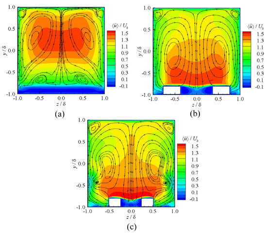
Figure 26.
Intensity maps of the mean streamwise velocity and superimposed in-plane cross-stream streamlines highlighting the secondary flow arising in a square channel roughened with V-shaped ribs of (a) 90°, (b) 60° and (c) 45°. Figures taken from Fang et al. [229].
The topology of the secondary flow in rectangular ducts of increasing aspect ratio was studied by Vinuesa et al. [234] using DNS of turbulent flow at friction and 360 with the aid of the SEM-based code NEK5000, where is defined in terms of the duct half-height h and the mean friction velocity , where represents the mean wall-shear stress averaged over the four duct walls (which is related to the pressure losses), and is the fluid density. Figure 27 shows the secondary flow structure in ducts of varying aspect ratio. Figure 27a,b depict the streamlines of secondary mean flow in a square and rectangular (of aspect ratio 1:3) conduit, respectively, at (blue contours) and (dotted red contours). For comparison, the black lines in Figure 27b show the first contour from the square duct at . Figure 27c shows the resulting vortex topology from a rectangular conduit of aspect ratio 1:5 (green contours) at . For comparison, superimposed streamlines for conduits of aspect ratios 1:1 (blue contours), 1:3 (dotted red contours) and 1:10 (dotted green contours) are shown at . The characteristic two-vortex pattern is shown on each corner and the tangent line between the vortices along the corner bisector. In the square channel, a symmetric pair of vortices is formed, which convect momentum from the duct center plane toward the bisector. In the rectangular channels, the symmetry is lost as the vortex below the bisector expands to the right occupying most of the cross-sectional area of the rectangular conduit. In general, as increases, the vortices become more elongated, and their centers move away from the wall. Vanderwel et al. [235] studied the instantaneous structure of secondary flows in a turbulent boundary layer using DNS based on a pseudo-spectral solver. The numerical results were compared with experimental data obtained for flow in a rectangular conduit with a roughened bottom surface created with LEGO bricks. They found that the secondary flows that formed were not very sensitive to the Reynolds number and that the DNS reproduced fairly well the experimental measurements regarding the mean flow and turbulent stress distributions.
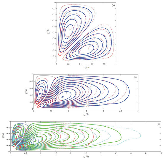
Figure 27.
Topology of the secondary flow generated in turbulent flow in rectangular conduits of varying aspect ratios: (a) streamlines in a square duct at (blue contours) and (dotted red contours), (b) streamlines in a rectangular duct of aspect ratio 1:3 at (blue contours) and (dotted red contours) and (c) streamlines in a rectangular duct of aspect ratio 1:5 at (green contours). The black lines in (b) show the first contour from the square conduit at , while the blue, dotted red and dotted green contours in (c) are streamlines from a square (1:1) and rectangular ducts of aspect ratio 1:3 and 1:10, respectively. Figure taken from Vinuesa et al. [234].
DNS models of turbulent flow in channels have been of great help in clarifying the physics behind the phenomena occurring in wall-bounded turbulent flows with a particular focus on the origin of Prandtl secondary flows of the first kind. As was outlined by Lanaers et al. [236], the occurrence of negative streamwise velocities in wall-bounded turbulence is a counterintuitive phenomenon. For example, simulations of the turbulent boundary layer for the zero-pressure gradient by Spalart and Coleman [237] revealed the occurrence of negative wall-shear stresses, confirming previous experimental findings of Johansson [238], who observed the existence of an instantaneous flow reversal. Later, Hu et al. [239] reported a similar phenomenon for turbulent flow in a channel. Alongside the flow reversal phenomenon, there is another rare event consisting of large fluctuations of the wall-normal velocity component, which can be up to an order of magnitude larger than their local standard deviation. These fluctuations are responsible for extreme flatness values of the wall-normal velocity [240,241,242,243]. The occurrence of negative streamwise velocities and extreme wall-normal velocity fluctuations in turbulent channel flow was investigated by Lanaers et al. [236], who performed DNS at , 590 and 1000. They observed the presence of flow reversal near the channel wall (i.e., negative wall-shear stress) and claimed that such backflow was not due to numerical artifacts. As increases from 180 to 1000, the intensity of the flow reversal is seen to increase from 0.01% to 0.06%. The strong oblique vortices that form outside the viscous sublayer are responsible for both the backflow (in the negative streamwise direction) and the transverse flow (in the negative spanwise direction). Extreme wall-normal velocity fluctuations were also observed, which are responsible for the high flatness values near the wall. The flatness values also increase with increasing .
Kaldy and Ayala [244] conducted numerical simulations addressing the assessment of secondary flow characteristics in pipe bends under several different conditions, using the turbulence closure available in the CFD module of COMSOL Multiphysics 5.1. In particular, they analyzed the flow at , 1000, 10,000 and 100,000 in pipe elbows with curvature ratios , 0.154 and 0.67. The flow characteristics were quantitatively assessed at sweep angles , and within the bend. They confirmed previous findings that as increases, the maximum vorticity increases and the core of the vortical structure moves closer and closer to the pipe wall due to inertial forces. Contrary to the rational belief that the lower the value of , the longer the fluid takes to develop within the bend, they found that lower values of the secondary flow velocity and vorticity occur at lower values of due to the lower centrifugal acceleration felt by the fluid. Yao et al. [245] analyzed the modulation of the amplitude of wall-bounded turbulence using DNS of turbulent channel flows at , 1000 and 2000. The tail of the probability density function of the wall-normal velocity is characterized by extreme rare events in the form of near-wall fluctuations of unprecedented high levels. Yao et al. [245] observed that by taking the conditional average of these near-wall fluctuations, a pair of counter-rotating, large-scale vortices associated with modulation are revealed, which, in turn, can induce strong sweep motions and form a high-speed region in between. Chin et al. [246] reported further DNS of turbulent channel flow at to investigate the flow topology about a critical point pair in the skin-friction field in turbulent flows over walls. The existence of such critical points was demonstrated by Chong et al. [247], which were termed by Chong et al. [248] as “no-slip” critical points, and defined as points over the walls where the skin friction in the streamwise and spanwise directions is simultaneously zero. Therefore, these points represent points of local separation in the flow field. Chin et al. [246] found that the skin friction patterns around critical points resemble the three-dimensional U separation proposed by Perry and Chong [249]. The conditional average of the velocity field above a pair of critical points revealed a strong spanwise vortex above, with further vortical activity downstream. The structure and dynamics of backflow in turbulent channel flows were also studied by Cardesa et al. [250] for in the range between 547 and 2003. Their numerical results show that any increase in the volume fraction of backflow for a given wall distance occurs together with an increase in the number of backflow structures per surface area.
5.1.3. Pipe Swirling Flow Modeling
It is well known that in axially rotating pipes, additional forces and complexities arise that affect the flow properties compared to stationary (non-rotating) pipes. The centrifugal forces generated in the flow due to the solid-body rotation of the pipe wall produces a flow redistribution in the spanwise direction that causes a secondary flow accompanied by a nonuniform streamwise flow pattern and an increase or decrease in the pressure drop. As was pointed out by Speziale et al. [251], the main interest in studying axially rotating pipe flows lies in the case of fully developed turbulent flows because in the laminar regime the flow remains essentially unidirectional with a parabolic velocity profile similar to that occurring in a non-rotating pipe. Accordingly, in a turbulent regime, the mean flow is no longer unidirectional with a non-zero azimuthal mean velocity component when viewed in a reference frame at rest with the pipe. Induced secondary flow in rotating pipes enhances mixing and improves heat transfer rates, which is of great value in many cooling and heating systems as well as in turbo-machinery applications, such as pumps, turbines and compressors, which rely on rotating pipes for optimization and design purposes of these systems.
Early numerical simulations of rotating pipe flows, with the use of a variety of turbulence closures, were performed by Kikuyama et al. [252], Hirai et al. [253], Eggels and Nieuwstadt [254], Malin and Younis [255] and Orlandi and Fatica [256]. In particular, the simulations performed by Hirai et al. [253] showed that the standard turbulence closure does not accurately describe turbulent flow in a rotating pipe and that better predictions will require the use of a full RSM approach. On the other hand, the calculations reported by Eggels and Nieuwstadt [254] apply to moderate swirling numbers; therefore, they were not able to predict the experimental observation of flow relaminarization occurring at high values of S. The results of FVM simulations reported by Malin and Younis [255], using two RSM approaches to deal with fully developed flow and heat transfer in an axially rotating pipe confirmed the findings of Hirai et al. [253] on the better performance of the RSM approach to describe the influence of pipe rotation, including the suppression of the radial turbulent transport of heat and axial momentum and the deformation of the axial velocity profile toward a laminar-like shape. A further important addition to early published work on rotating pipe flow was presented by Orlandi and Fatica [256], who performed highly resolved DNS using FD techniques. They found that when the pipe rotates, a degree of drag reduction is achieved in agreement with experimental findings, which appears to be related to a modification of the vortical structures near the wall. Numerical simulations reported by Speziale et al. [251] have shown that second-order closure models can successfully predict the emergence of a rotationally dependent axial mean velocity accompanied with the presence of a mean swirl motion relative to the rotating pipe wall. Good evidence was also provided that the mean swirl velocity is generated by a nonzero shear component of the Reynolds stress tensor, which at high is confined to the region near the wall.
Feiz et al. [257] performed FD-based simulations of fully developed, incompressible turbulent flow in stationary and rotating pipes at and 7400 for swirling numbers and 2, using a LES approach to assess the performance of two different subgrid scale models, namely, a dynamic model and the Smagorinsky model. For the same values of and S, their results were compared with the DNS-based simulations by Orlandi and Fatica [256] and the experimental measurements by Reich and Beer [136]. The LES approach was observed to capture reasonably well all flow features in both rotating and non-rotating pipes provided that it is complemented by the dynamical model. Despite some discrepancies with Orlandi and Fatica’s [256] results, LES was able to predict the gradual decrease in turbulence intensity as the pipe rotation increases due to the stabilizing effects of centrifugal forces. Preliminary studies of swirling and non-swirling flow in and bends at = 50,000 for were carried out by Pruvost et al. [258] to approach the flow in a torus reactor. They used the commercial software FLUENT to solve the Navier–Stokes equations with various turbulence models and three types of near-wall modeling strategies, using a wall function and a low-Re model with boundary layer resolution. Acceptable results when compared with experimental data for were achieved using the model and the wall function. However, the low-Re model revealed to be sufficiently accurate for the modeling of swirling flow in bends at coarser grid resolutions. Further simulations by these authors showed that the flow structure at the bend outlet depends on the swirl intensity. For instance, the flow results in a rather complex interation between swirl motion and Dean vortices for . For S between 0.2 and 0.3, the influence of the swirl motion is such that the Dean vortices disappear, while at higher S, the swirl motion dominates, and the flow is only barely affected by the pipe curvature.
A new flow problem was advanced by Nygård et al. [259], who modeled the effects of a rotating pipe on turbulent flow by prescribing a circumferential mean pressure gradient, which induces a tailor-made azimuthal mean velocity near the wall. The induced swirl is introduced in the tangential momentum equation by adding a pressure gradient near the wall (i.e., for , where R is the radius of the circular pipe) to the total tangential pressure gradient. They performed DNS of flow at for three different normalized swirl-inducing pressure gradients: 0.0125, 0.025 and 0.05, corresponding approximately to swirl numbers S of 0.45, 0.60 and 0.85, respectively. Their results reveal that a skewing of the coherent near-wall structures is induced by the emerging azimuthal mean velocity, while the flow resistance increases for the low-swirl case (i.e., for ) and the drag gradually reduces as the swirl is increased. However, the skewing of the coherent near-wall structures alone is not sufficient to reduce the wall friction. Nygård et al. [259] further suggested that controlling the streaky structures of the axial velocity fluctuations may represent a way to temper turbulence. Visualization of the instantaneous axial and radial velocity fluctuations clearly shows that one effect of the skewed mean flow is to tilt the streaks of high- and low-velocity fluid (see their Figures 8 and 9 ). In the case of low swirl, the tilted streaks are seen to increase the drag, while, in contrast, they result in drag reduction in the cases of larger swirls.
Recently, Davis et al. [260] conducted DNS of turbulent flow in a rotating pipe at = 19,000 and S ranging from 0 to 3, with the help of the open source SEM solver Nek5000. In addition to providing turbulence statistics, these scholars used the POD method to identify the relevant highest-energy modes of the flow and gain insight into the flow coherence. Under the effects of pipe rotation, they observed a redistribution and reorientation of the Reynolds stress tensor, implying significant changes in the flow topology particularly at large values of S as well as in the organization (i.e., coherence) of the flow. Further DNS of incompressible, turbulent flow in rotating circular and cylindrical concentric pipes was performed by Dunstan [261] using the Nek5000 code. In this study, flow along a rotating pipe was simulated at and 5300 with , 0.5, 1 and 2, while in the concentric pipe flow at with inner wall rotation rates , 0.2145, 0.429, 0.858 and 2 was considered. The simulations for flow in a rotating pipe have confirmed quasi-relaminarization of the flow accompanied by increased turbulent kinetic energy. As in early experiments by Taylor [61] with the inner and outer walls rotating in opposite directions, a counter-rotation flow is present even when only the inner wall is in solid-body rotation. This occurs at the same radial position in the gap span independently of the rotation rate S and radius ratio , where is the radius of the inner concentric cylinder, and is the radius of the outer concentric cylindrical pipe. Figure 28 shows the wall streaks near the inner rotating wall for , 0.429 and 2. For the steady inner wall case (), the streaks are oriented with the main stream, while an obvious tilting of the wall streaks are clearly seen for and 2. These results confirm previous findings by Nygård et al. [259], where similar streak tilts were observed near the walls of a circular cross-sectional rotating pipe. For the case, Dunstan [261] reports streaks tilted at with respect to the streamwise direction (see Figure 28c).
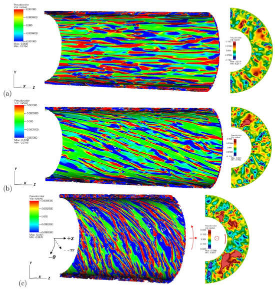
Figure 28.
Intensity maps of the instantaneous radial velocity fluctuations for the concentric pipe with inner wall rotation: (a) (non-rotating case), (b) and (c) . The plots on the right side correspond to sectional images of the left intensity maps. The flow orientation in all cases is along the -direction as indicated by the cylindrical coordinates (r,,z). The red chirality arrows in (c) apply to (b) also and indicate the streamwise flow direction and the rotation sense of the inner wall, while the black arrows also indicate the flow orientation and the tilted angle of the streaks. Figure taken from Dunstan [261].
5.1.4. Pulsatile Flow Modeling
In general, pulsatile flow can be defined as an unsteady flow in which a periodically varying time-dependent component is superimposed to a mean flow component. In this sense, a pure oscillatory flow can be regarded as a special case of pulsatile flow for which the mean flow component is zero. For a brief overview of pulsatile flow theory and a review of early analytical and numerical work, the reader is referred to the papers by Gündoğdu and Çarpinlioğlu [262,263] and references therein. A theoretical discussion on pulsatile flow in the laminar, transitional and turbulent regimes is provided along with the support of experimental data available at that time. The same authors later presented a review devoted entirely to work on pulsatile flow in pipes prior to 2001 [264]. As described by Çarpinlioğlu and Gündoğdu [264], the theory of laminar pulsatile flow seems to be completely founded, while further experimental and numerical work is needed to fully understand the behavior of pulsatile flow under transitional and turbulent conditions. Apparently, the same claim is still valid today since the number of numerical simulations on pulsatile pipe flow is still tiny compared to the total number of simulations of turbulent flow in pipes.
A fundamental parameter in studies of oscillatory and pulsatile flows is the frequency, , and the dimensionless Womersley number, which measures the importance of the time rate of change of the momentum relative to the viscous forces. For , the oscillation period is larger than the viscous diffusion time, and the flow is a quasi-steady Poiseuille flow in phase with the pressure gradient. At higher values of , the flow velocity begins to exhibit a phase delay with respect to the pressure gradient [265,266,267]. Hellström and Fuchs [268] simulated steady and pulsatile flow in a pipe bend and a double-bended pipe using the RANS and LES modeling approaches with a second-order monotone advection and reconstruction scheme (MARS). A comparison of the velocity profiles with experimental measurements for the single-bended pipe shows that at the bend exit, LES performs better than RANS, also providing more details about the flow dynamics. For both approaches, the flow field downstream of the bend was seen to be sensitive to different types of small amplitude secondary flow as a consequence of small uncertainties in the pipe inlet conditions. In the double-bended pipe, the LES calculations describe qualitatively well the behavior of the flow field compared to the RANS computations. In particular, downstream of the second bend, the flow is entirely dominated by swirling motion and the Dean vortices formed from the second bend, whose strength varies with the amplitude of the axial velocity. The RANS model was able to predict only a pair of Dean vortices at the outlet of the second bend, while up to four vortices were seen at certain moment with the LES calculations.
The effects of pulsation on secondary flow development were later studied by Timité et al. [269], who used FLUENT-based simulations of pulsated water flow at 300 K in a pipe bend. The results of their simulations were compared with in-house LDV measurements for and . The inlet flow velocity was defined as
where is the mean flow velocity, is the peak oscillatory velocity and is the circular frequency. Values of between 0.5 and 1.85 were used. The numerically obtained axial velocity profiles at the bend exit for steady flow are in very good agreement with those obtained experimentally with an average deviation of only 2%. Figure 29 shows the corresponding axial velocity profiles for pulsatile flow at , and and moments , and . The profiles in the y-plane resemble those obtained for steady flow, while in the x-plane, the maximum fluid velocity occurs near the outer pipe wall, and a reverse flow is evident toward the inner wall particularly for . However, when is increased to 17.17 by keeping all other parameters the same, the amplitude of the reverse flow intensifies near the inner wall (see Timité et al.’s [269] Figure 14). The average deviation between the numerical and experimental velocity profiles in Figure 29 increases to %. When the amplitude of the flow oscillatory component , the secondary flow structure becomes much more complicated. Figure 30 shows the visualization of the secondary flow patterns at the bend exit for and varied values of , and . For and , a siphon phenomenon is observed in the center of the cross-sectional plane for , which attains its maximum at . In this case, the secondary flow consists of only one vortex (or a swirl). When , the Lyne flow instability appears earlier within the elbow with maximum amplitude close to the pipe center for at . The intensity of the secondary flow decreases with increasing during the flow acceleration phase. Oki et al. [158] presented further numerical simulations of pulsatile flow in a square section double-bended exhaust pipe. The results of their simulations compared favorably well with experimental data of airflow shown in Figure 17.
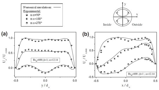
Figure 29.
Axial velocity profiles obtained numerically (symbols) as compared with experimental data (solid lines) for pulsatile flow at the exit plane of a 90° pipe bend at , , and varying moments : (a) y-plane and (b) x-plane. Figure taken from Timité et al. [269].
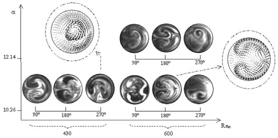
Figure 30.
Intensity maps of the secondary flow patterns for pulsatile flow at the exit of a pipe bend for and varied frequency parameters ( and 12.14; and 600; , and ). Figure taken from Timité et al. [269].
DNS and LES of pulsating turbulent flow in a channel were also presented by Scotti and Piomelli [270] for a wide range of frequencies of the driving pressure gradient. They found that the fluctuations generated in the near-wall region by the unsteady pressure gradient do not propagate beyond a certain distance from the wall, while no substantial departure from the Stokes regime was observed at high frequencies. Recently, Mirfendereski and Park [271] performed DNS coupled with the immersed boundary method to study pulsatile flow in a planar channel with single and double one-sided semicircular constrictions at and 1000. Such configuration model is relevant for blood flow in large arteries with stenoses. They found that the double constrictions lead to intense and broadband downstream turbulence, which promotes critical wall-shear stresses in the post-stenotic areas. Also, multiple strong recirculations were observed between two stenoses, implying that this area is highly prone to atherosclerosis progression.
Yapıcı and Albayrak [272] performed two-dimensional simulations of steady-state water flow in a circular pipe subjected to external heating with a uniform and non-uniform wall heat flux, using the Fluent 4.5 and HEATING7 computer codes. They provided details of the temperature and thermal stress distributions inside the pipe wall. For non-uniform heating and mean flow velocities of 0.05 and 0.1 m s−1, the results indicate maximum inner wall temperatures of 31 °C and 19.5 °C, respectively. For uniform heating, the inner wall temperature increases almost linearly along the pipe length, while for non-uniform heating, the temperature increase is non-linear and reaches its maximum value after half of the pipe. For a pipe of length 1 m, this value occurs at 0.58 m from the inlet when the mean flow velocity is 0.1 m s−1. In a more recent work, Marugán-Cruz et al. [273] used collocation spectral methods to simulate heat transfer and thermal stresses in a thin-wall circular pipe under non-uniform heat flux. They studied the role played by , and the Biot number, defined as
where is the convective heat transfer coefficient between the fluid and the solid, is the thickness of the pipe wall and is the conductivity of the solid wall. They found that for , the maximum thermal stresses concentrate in the adiabatic side of the pipe, while for , they appear near the peak heat flux, i.e., in the hot side of the pipe. For the range 0.1 ≲ Bi ≲ 0.3, the thermal stresses are approximately uniformly distributed along the pipe circumference of the inner wall. Recently, Kırmızıgöl et al. [274] conducted a conjugate heat transfer analysis of the cooling systems in low pressure die casting. A good level of accuracy was demonstrated by comparing the numerical results with available experimental data.
5.2. Pipe Flow Modeling Using Particle-Based Methods
Smoothed Particle Hydrodynamics (SPH) is probably the most successful particle-based method due to its numerous applications in different areas of science and engineering. However, being relatively young compared to conventional mesh-dependent methods, the number of published articles dealing with SPH simulations of pipe flow is considerably lower. One of the first formulations of SPH to solve the Navier–Stokes equations for a viscous fluid flow was reported by Takeda et al. [275], who successfully assessed the accuracy of the method in calculations of two-dimensional (planar) Poiseiulle flow between two parallel plates and Hagen–Poiseuille flow in a circular cylindrical pipe. They presented numerical solutions for the steady-state velocity profiles that agree well with the analytical solutions. The time-dependent, plane Poiseuille flow between stationary infinite plates at was later simulated by Morris et al. [276]. They obtained numerical velocity profiles that were in close agreement with the analytical series solution for plane Poiseuille flow. The deviations reported from the analytical solution across the channel were all within 2%, and the maximum deviation from the steady-state () solution was approximately 0.7%. Watkins et al. [277] performed a first attempt to solve the Navier–Stokes equations in full by writing in SPH form the viscous stress tensor. They simulated plane Poiseuille flow at , finding a good matching with the analytical stready-state solution. However, they noticed that working with , the Poiseuille flow becomes turbulent and a simulation of such a flow should become unstable. They tried a calculation with , which, slightly after achieving a stationary state, the solution became unstable with the instability rapidly spreading throughout the entire computational domain.
Additional SPH simulations of time-dependent Poiseuille flow were reported by Pozorski and Wawreńczuk [278] and Sigalotti et al. [279]. In particular, Pozorski and Wawreńczuk [278] used a projection method to enforce the zero-divergence constraint for the simulation of incompressible viscous fluid flows. From their Figure 5b, the correspondence between the numerical and analytical solutions for the time-dependent plane Poiseuille flow is quite satisfactory. A different SPH formalism, which works equally well for both compressible and incompressible viscous flows, was introduced by Sigalotti et al. [279]. Unlike other SPH formulations at that time, their scheme involved direct evaluation of the viscous stress tensor combined with the pressure-gradient correction advanced by Morris et al. [276]. The method was found to reproduce the analytic series solution for unsteady plane Poiseuille and Hagen–Poiseuille flows at very low and moderate Reynolds numbers. For plane Poiseuille flow at , the steady-state solution was achieved at 1 s. At this time, the relative error between the numerical and analytical asymptotic maximum velocity was found to be within %, while in the course of the simulation, the maximum and minimum densities were found to be between and , respectively, implying that the incompressibility of the flow is very well reproduced by the numerical scheme. In order to compare with the results of Watkins et al. [277], an additional run was carried out at . Figure 31 shows the results for the transient evolution until a steady-state is reached at 230 s. The solution remained perfectly stable with a relative error of about 0.35% when compared with the analytical solution and density variations in the interval in the course of the simulation. The numerical solution of the time-dependent Hagen–Poiseuille flow was also found to reproduce very well the analytical flow solution at . The effects of the number of particles, the number of particle neighbors and the timestep value on SPH simulations of Hagen–Poiseuille flow have been studied by Wonjoo et al. [280].
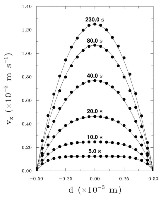
Figure 31.
Numerical axial velocity profiles (filled dots) compared to the analytical solution (solid lines) for the time-dependent plane Poiseuille flow at . The steady-state solution is reached at 230 s. Figure taken from Sigalotti et al. [279].
It is clear from the simulations above that the first applications of SPH to pipe flow modeling were dedicated to assessing the performance of the method against the simple case of laminar flow through a cylindrical pipe, using as benchmark test cases the plane Poiseuille and the Hagen–Poiseuille flow. After consolidating the effectiveness and accuracy of the method, it began to be used in the simulation of more complex pipe flows. A relatively early example was provided by the work of Klapp et al. [281], who performed exploratory calculations of the flow of a single phase viscous fluid through a wellhead choke of real dimensions using the open source code TREESPH, which was widely employed for the modeling of astrophysical flows. Their results were qualitatively in agreement with theoretical expectations for flow converging to a narrow throat. An approximately stationary flow pattern was rapidly established throughout the tube, with the density and pressure dropping and the mean axial flow velocity rising within the choke throat. Hou [282] developed a SPH formalism for solving the Navier–Stokes equations with applications to rapid pipe filling and emptying, isolated slugs traveling in an empty pipe and flow separation in a pipe bend. In particular, the results of one- and two-dimensional SPH calculations show that the flow separation at the bend has a major effect on the local pressure magnitude and distribution, with technical implications on slug impact at a sharp bend.
Particle-based methods, such as SPH, show a superior performance compared to conventional Eulerian mesh-dependent methods in the simulation of complex flows involving free surfaces and moving bodies. However, they have shown some difficulties in the treatment of permeable and non-reflecting boundary conditions. As outlined by Lastiwka et al. [283], the simulation of fluid flow in truncated pipes requires the implementation of proper boundary conditions for inflow and outflow. In general, stationary inflow and outflow fluid regions are naturally described in a Eulerian frame of reference, while a Lagrangian frame moves with the fluid particles, which may take a short time to flow into and out of a domain. Some early SPH simulations of Poiseuille flow have been carried out using periodic boundary conditions at the inlet and outlet planes of a pipe. Since their use implies recycling the particles through the domain, any small perturbation will amplify over time severely degrading the solution. This explains why SPH simulations of pipe flow have been mainly limited to laminar flows. However, this limitation has motivated quite a bit of research work in the last decade on the accurate implementation of inflow and outflow boundary conditions in SPH [283,284,285,286,287,288]. Most effort has focused on removing undesirable wave reflection from the outlet boundary. For example, Lastiwka et al. [283] implemented an inflow zone from which particles are inserted into the fluid domain as needed, while particles crossing the outlet plane are moved into an outflow zone using a characteristic-based analytical framework adapted in SPH from mesh-based methods. More recent work on the derivation of non-reflecting outlet boundary conditions rely on an outgoing wave equation to move the particles in the outflow zone [285]. A scheme based on the method of characteristics using the Lagrange interpolation in the time domain was also devised by Wang et al. [286] to calculate the pressure and velocity of outflowing particles. In the context of wind-tunnel-like simulations, Negi et al. [287] proposed a hybrid approach where the method of characteristics is combined with a simpler frozen-particle (do-nothing) technique for weakly compressible SPH. Bui and Nakata [288] proposed a further non-reflecting boundary condition for viscous open-channel flows based on a hybrid scheme that combines an in/outflow algorithm with periodic boundary conditions. All of these approaches were assessed for turbulent flow conditions and found to considerably reduce spurious noisy waves incident from the outlet when anisotropic flow is convected through it.
Ting and Yeak [289] used an improved SPH formulation based on two different wall boundary approaches, namely, a single-layered and a double-layered virtual particles. They presented a comparison between both approaches for plane Poiseuille flow at , concluding that the double-layered treatment leads to a steady-state velocity profile with the smallest error when compared to the analytical series solution. More recently, Liu and Liu [290] tested the performance of a SPH formalism based on two different ways to deal with the viscous stress tensor on plane Poiseuille flow at and 5. In the first approach, the viscous stress tensor is evaluated using a full SPH approximation, while the second scheme relies on a combination of SPH and FD approximations for the viscous stress tensor. They found that the second method is more stable than the first one after the flow approaches the steady-state solution for flow at , while both schemes remain stable for . These results contradict previous findings by Basa et al. [291], who employed different viscous force formulations, boundary condition implementations and particle inconsistency corrections in SPH simulations of plane Poiseuille flow, concluding that failure of the method cannot be avoided for moderate () and higher Reynolds numbers. They pointed to transverse fluctuations as the source of the instability in agreement with previous studies [277,279]. However, Song et al. [292] demonstrated that the documented instability can be avoided for a wide range of values if ratios of the smoothing length to the particle spacing greater than about 1.5 along with a density re-initialization technique are used. In a very recent work, Yang et al. [293] performed SPH test simulations of plane Poiseuille flow at between 20 and 1000, obtaining stable radial velocity profiles that were in very good agreement with CFD simulation data and theory (see their Figure 6). Compared to the CFD results, the SPH profiles slightly overestimate the velocity near the pipe wall due to SPH failure to strictly enforce the no-slip boundary condition, which will certainly need further investigation.
Only recently did SPH begin to be applied to more complex pipe flows such as flow in a bend [294], in curved pipes with different geometries [295] and in Venturi meters [15]. In particular, Sigalotti et al. [294] reported highly resolved SPH simulations of laminar and turbulent water flow in a pipe bend, using a LES turbulence model. The performance of the numerical results was assessed by direct comparison with experimental data provided by Enayet et al. [120]. For laminar flow at and 1093, the axial velocity profiles upstream of the bend and the cross-sectional velocity maps within the bend were found to reproduce the experimental data with root-mean-square errors % (see their Figures 4–6). Figure 32 shows the turbulence intensity profiles at different spatial resolutions as compared with Enayet et al.’s [120] experimental data (Figure 32a) and cross-sectional streamwise velocity maps within the bend and in the downstream tangent (Figure 32b) for flow at =43,000. Although asymptotic convergence to the experimental data for the velocity profiles was achieved with 4 million particles for both laminar and turbulent flows, it was necessary to increase the number of particles to 16 million to obtain a similar level of convergence for the turbulence intensity profiles. Further SPH simulations coupled with a LES model were carried out by Alvarado-Rodríguez et al. [295] for different pipe geometries, including U-bends, S-shaped pipes and helically coiled pipes. In this case, the performance of the simulations was also assessed against experimental measurements. For the different pipe geometries and values considered, the maximum deviations between the experimental and numerical velocity profiles were always within %. The contour shapes and the swirl intensities were also found to display very similar characteristics to the experiments. The authors concluded that the very good agreement displayed with the experimental data demonstrates the uprising capabilities of SPH methods for tackling complex swirling flows in bends and manifolds.
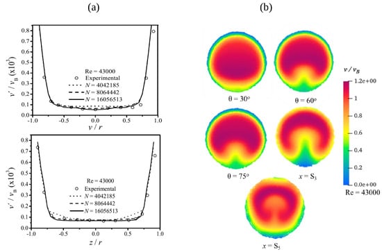
Figure 32.
(a) Numerical turbulence intensity profiles in the horizontal plane (top) and vertical plane (bottom) at 0.58 pipe diameters upstream of a bend for different particle resolutions as compared with Enayet et al.’s [117] experimental measurements and (b) cross-stream velocity maps at angular planes , and within the bend and at and pipe diameters downstream of the bend outlet. Figures taken from Sigalotti et al. [294].
Venturi meters are tubular devices consisting of convergent and divergent sections connected by a constricted pipe (or throat). They are widely used in many industrial applications and in laboratory experiments to measure the volumetric flow rate, Q, of a fluid in a pipe. As the fluid flows through the convergent section and enters the throat, its velocity increases, resulting in an effective pressure drop according to Bernoulli’s principle. Most early and recent numerical simulations of single-phase fluid flow through Venturi meters have been performed using conventional mesh-dependent methods [296,297,298,299,300,301,302], while apparently the only work so far published using SPH techniques has been reported by Sigalotti et al. [303]. They carried out numerical simulations of water flow through a Venturi tube of rectangular cross-section (see Figure 33) at = 13,272 (for liters per minute (lpm)) and 33,180 (for lpm), using a modified version of the open-source code DualSPHysics coupled to a LES turbulence closure. Working with 4 million SPH particles, they predicted centerline velocity profiles across the convergent-divergent sections that matched in-house experimental measurements with errors varying from 4.3% (for 10 lpm) to 7.1% (for 25 lpm), while the differential pressure was predicted with errors of 1.4% for 10 lpm and 6.8% for 25 lpm. Cross-sectional velocity profiles within the throat and divergent section differed by no more than 5.5% from the experimental data. Figure 33 depicts the SPH flow structure along the Venturi meter for (a) 15 lpm and (b) 25 lpm as compared with the experiment. The velocity fields look quite similar with small differences close to the inlet and outlet of the Venturi tube. The DualSPHysics toolbox was also recently used by Suntarto et al. [304] to study the flow through straight channels with rough walls at , 50 and 100. They performed simulations for varying heights of the roughness, corresponding to 0.05, 0.1 and 0.2 times the channel width, and different geometries, consisting of semicircular, triangular and rectangular ribs. It is found that the roughness of the wall affects the mainstream flow velocity in that its maximum value is no longer aligned with the axis of the pipeline, as occurs in the Poiseuille flow with smooth pipe walls. In addition, the wall friction factor was found to depend on the roughness shape, with the triangular ribs producing the smallest friction and the rectangular ones contributing with the greatest wall friction coefficient.
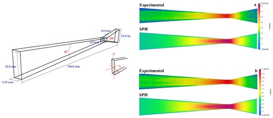
Figure 33.
(Left) Schematic view of the Venturi flow meter used in the experiments and SPH simulations. (Right) Experimental and SPH mainstream velocity maps for (a) 15 lpm and (b) 25 lpm. Figures taken from Sigalotti et al. [303]. https://creativecommons.org/licenses/by/4.0/ (accessed on 12 March 2025.)
6. Flow of Non-Newtonian Fluids in Pipes
In this section, we discuss published work on experimental and theoretical work on pipe flow of non-Newtonian fluids. In general, the flow of non-Newtonian fluids exhibits physical properties that differ in many ways from those of Newtonian fluid flows. A notorious difference is that the viscosity of non-Newtonian fluids depends on the shear rate and, in most cases, on the shear rate history. The relation between the shear stress, , and the shear rate, , defined by the constitutive relation
is no longer linear and can even depend on time. In other words, the apparent viscosity, defined as the ratio between the shear stress applied to a fluid and the shear rate, varies with temperature and pressure and depends on the flow conditions such as, for example, the flow geometry and the shear rate and sometimes even on the kinematic history of the fluid. The type of fluid is, in general, grouped into the following three categories: (a) inelastic, purely viscous or time-independent fluids, for which the shear rate at any point and instant is determined by the shear stress at that point and instant, (b) time-dependent fluids for which the relation between the shear rate and the shear stress depends on the duration of shearing and the kinematic history of the fluid and (c) viscoelastic fluids, which exhibit properties common to ideal fluids and elastic solids and show only partial elastic recovery under deformations. However, most existing analyses deal with time-independent non-Newtonian fluids because they are the simplest to model. Depending on the form of Equation (50), time-independent non-Newtonian fluids can be in turn divided into shear-thinning (or pseudo-plastic), shear-thickening (or dilatant) and visco-plastic. For a complete description of this type of fluid flows, the interested reader is referred to the book chapter by Nguyen and Nguyen [305]. In particular, the most common type of time-independent non-Newtonian fluids encountered are pseudo-plastic fluids.
Several models exist in the literature to explicitly write Equation (50). For example, shear-thinning behavior is characterized by a decrease of the apparent viscosity with increasing shear rate and can be represented in a first approximation by the power-law model, , for . For , the fluid shows Newtonian behavior, while for , it exhibits shear-thickening behavior. Other viscosity models exist that describe better the fluid behavior at very low and very high shear rates as, for example, the Carreau [306], the Cross [307] and the Ellis fluid model. On the other hand, visco-plastic fluid behavior is characterized by the existence of a yield stress, , which must be exceeded before the fluid starts flowing or deforming. The Bingham plastic model and its generalization, known as the Herschel–Bulkley fluid model, are widely used constitutive relations used to describe pseudo-plastic fluids. However, many biological fluids, especially blood and foodstuffs, are better described by the Casson fluid model. Kassim and Sarow [26] present a review of viscous fluid flows in the food-processing industry, focusing on the rheology and movement of syrups and particularly honey, which is a more complex fluid. Contrary to pseudo-plastic fluids, dilatant fluid behavior is characterized by an increase in the apparent viscosity with increasing shear rate. For this class, the available information is more limited, and, as for the pseudo-plastic fluids, it can be described by the power-law model with , which in terms of the apparent viscosity can be written as , implying that the viscosity increases with increasing shear rate.
6.1. Generalized Reynolds Number and Friction Factors for Non-Newtonian Fluid Flow in Pipes
A similar expression to Equation (1) holds for the Reynolds number for a non-Newtonian fluid flow in a pipe but now in terms of the apparent viscosity , which for pipe flow is given by
where is the shear stress at the pipe wall, v is the mainstream flow velocity and D is the pipe inner diameter. In general, is a useful quantity for specifying the correlation between flow rate and pressure gradient for non-Newtonian flow in pipes [305]. Therefore, the generalized Reynolds number can be written as
Noting that for laminar fluid behavior , Equation (52) can be rewritten as [308]
where for Newtonian behavior and so that Equation (53) reduces to Equation (1).
The friction factor for laminar non-Newtonian flow obeys the same mathematical expression as for laminar Newtonian flow, i.e., but with defined by Equation (52). According to the stability analysis of Ryan and Johnson [309], the critical value for which the transition from laminar to turbulent flow occurs for inelastic non-Newtonian fluids is a nonlinear function of the power-law index n (see Nguyen and Nguyen’s [305] Figure 5). In particular, for pseudo-plastic fluid flows in pipes, the critical value of occurs between 2100 and 2400 for , while for dilatant fluid flows (n > 1), this value decreases monotonically from 2100 for to about 1700 for . On the other hand, Dodge and Metzner [310] derived the implicit correlation
for the turbulent flow of pseudo-plastic fluids. Early work addressed to derive friction factor correlations for the laminar flow of inelastic non-Newtonian fluids in non-circular ducts, including square, rectangular and triangular cross-sections, has been reported by many scholars [311,312,313,314,315,316,317,318,319]. Based on similarity conditions, Tomita [311] derived the following relationship for turbulent flow
where is given by Equation (53). On the other hand, Kozicki et al. [315] derived the friction factor correlation for turbulent flow in pipes of arbitrary cross-sectional shapes
where a and b are two length parameters characterizing the pipe cross-section, and is a generalized Reynolds number given by
with being the hydraulic diameter of the non-circular pipe. Note that for a circular pipe ( and ), Equation (56) reduces to Equation (54). Later on, Delplace and Leuliet [320] pointed out that the pressure drop prediction for laminar flow of pseudo-plastic fluids in straight ducts of arbitrary cross-sections requires a further generalization of Equation (57). They proposed the following generalized Reynolds number
where . For a circular pipe, , and Equation (58) reduces to Equation (57) for and as is appropriate for a circular cross-section. Appropriate values of for infinite parallel plates, rectangular pipes, concentric annuli, isosceles triangular ducts and elliptical ducts are listed in Table 1 of Ref. [320] for different aspect ratios. Moreover, Hanks and Ricks [321] deduced an expression for the friction factor of power-law fluids under transitional and turbulent flow regimes, while Szilas et al. [322] derived by analytical means an expression which takes into account the effects of relative pipe wall roughness. For smooth walls, their F- relationship has the form
where is again given by Equation (53). Tomita [311] also derived F- correlations for the laminar flow of Bingham plastic fluids. A theoretical analysis of Bingham plastic fluids was also presented by Hanks and Dadia [323], while Hanks [324] performed an analysis of the transitional and turbulent flow of Herschel–Bulkley fluids. Other friction factor relationships for non-Newtonian fluids in pipe flow, including those just mentioned above, can be found in the review paper by García and Steffe [325], who presents a summary and comparison of F- correlations derived before 1986. Head losses for non-Newtonian fluids in straight and curved pipes were further discussed by Khan [326], while Havlik and Vycital [327] studied the rheological behavior of dense non-Newtonian time-independent slurries by describing them in terms of three simple models: a power-law model, a Bingham model and a yield-power-law model. They demonstrated experimentally that the kaolin slurries follow the yield-power-law model and that their laminar flow can be predicted using the friction factor relationship
where is the ratio of the yield value of the shear stress, , and the shear stress at the pipe wall, , and the Reynolds number is defined as
A F- correlation for turbulent pipe flow of non-Newtonian fluids, applicable to crude oils and petroleum products was proposed by El-Emam et al. [328]. They showed that their equation can determine the friction factor for any crude oil transported by pipelines more accurately than other published correlations. Fitton [329] suggested that the Colebrook–White relation (16) with replaced by can be used to predict the laminar/turbulent transition flow of Herschel–Bulkley fluids in an open channel, where is the hydraulic radius of the channel, provided that the Reynolds number is calculated according to
where is the yield stress of the fluid.
In a more recent work, Fialho Andrade et al. [330] provided friction factor relationships for the turbulent pipe flow of polymeric solutions using the Cross and Sisko models for the apparent viscosity. The derived friction factor correlations for the Cross and Sisko models were compared with the Prandtl–von Kármán resistance equation for Newtonian fluids, finding that for the range of considered the friction factors predicted from the non-Newtonian correlations showed values lower than those from the Prandtl–von Kármán equation. While most work on friction factor correlations for the laminar and turbulent pipe flow of non-Newtonian fluids has been limited to the case of smooth pipes, Dosunmu and Shah [331] derived a friction factor relationship that allows for accurate prediction of frictional pressure losses in rough pipes and annular sections. Their correlation reads as follows
where now f refers to the Fanning friction factor, is the outer diameter of the inner pipe, is the inner diameter of the outer pipe, is the equivalent diameter, is the roughness parameter, is the infinite friction parameter defined by , the parameter is given by , is the generalized Reynolds number given by Equation (53) and is the apparent viscosity at 511 s−1 in cP. Equation (63) was found to closely match the experimental friction pressure data in rough annular pipes. More recently, Assefa and Kaushal [332] have provided a direct comparison of selected friction factor correlations for all flow regimes of Bingham fluids. Their Table S3 contains a list of explicit correlations. The results indicate that for < 40,000, the correlations proposed by Wilson [333] and Morrison [334] produce a best fit to the experimental data. However, at higher values of , the deviation of the Wilson model from the experimental data is higher than that of the Morrison model. Figure 34 shows Morrison’s [334] Fanning friction factor as a function of for all flow regimes compared to experimental measurements for flow in smooth pipes [335]. Kamel et al. [336] presented a further recent comparative analysis of 19 Fanning friction factor equations for non-Newtonian fluid flow in pipes (see their Table 1). Friction factor correlations for fluids with power-law behavior index n from 0.14 to 1 (pseudo-plastic fluids) and ranging between 548 and 250,000 were statistically evaluated. Based on six different selection criteria, including the root-mean-square error and the Akaike information criterion, they concluded that El-Emam’s [328] friction factor correlation given by
for and can be recommended with a high level of confidence, followed by Dodge and Metzner’s [310] (see Equation (54)) and Szilas et al.’s [322] (see Equation (59)) correlations with a relative lower confidence level. In passing, we note that Gupta [337] obtained approximate solutions for the developing laminar flow of power-law fluids in pipes and straight channels by studying hydrodynamically equivalent Newtonian models. Sochi [338] derived an analytical expressions for the flow of Newtonian and power-law fluids in elastic circular pipes based on a lubrication approximation, and, more recently, Deterre et al. [339] derived by analytical means an approximate solution for the flow of power-law fluids in concentric annuli.
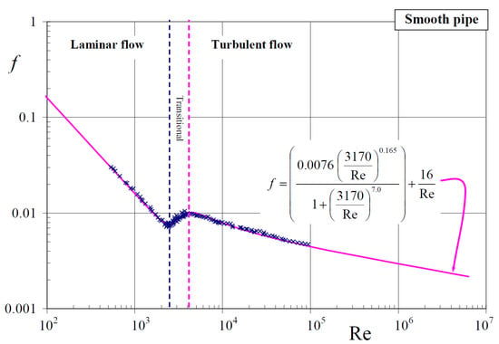
Figure 34.
Morrison’s [334] Fanning friction factor as a function of the Reynolds number for laminar, transitional and turbulent flow of Bingham fluids in smooth pipes (solid line). The symbols depict Nikuradse’s [335] experimental data. The mathematical expression of Morrison’s friction factor relationship is also depicted. Figure taken from Morrison [334].
6.2. Analytical Solutions
Analytical steady-state solutions for the flow of non-Newtonian fluids have been obtained by Kanuri et al. [340] for the laminar case and Nikushchenko et al. [341] for the turbulent case. In particular, Kanuri et al. [340] studied the Poiseuille flow in a channel of a second-grade fluid, which is a non-Newtonian fluid of viscoelastic type with a second-order relationship between shear stress and shear strain. Depending on the choice of second-grade fluid, they can exhibit both shear-thinning and shear-thickening. They solved the time-independent momentum conservation law
for an incompressible fluid (, where is a body force, and is the stress tensor for the second-grade fluid given by [342]
where and are fluid constants, and and are the first two Rivlin–Ericksen tensors [343], defined by
Using no-slip boundary conditions at the pipe wall and assuming that the maximum velocity occurs in the center of the channel, Kanuri et al.’s [340] steady-state solution for flow along the channel reads as follows
where , h is half the width of the channel, and x is the spatial coordinate along the main flow. The flow rate for the second-grade fluid was found to be . The steady-state profiles predicted by Equation (69) are of parabolic shape. On the other hand, Nikushchenko et al. [341] obtained analytical solutions for simple shear flows as well as the Blasius resistance law for the flow in a pipe. Their solutions in terms of velocity profiles are in good agreement with experimental data. Moreover, it is worth noting that an analytical solution for fluid motion in a cylindrical pipe has been presented by Khudjaev [344], which takes into account both the molecular and molar exchange of momentum between layers of the flow. In this case, third-order terms are formed in the Navier–Stokes equations.
6.3. Experimental Studies
Experimental research on pipe flow of non-Newtonian fluids started to be documented in the literature from the late 1970s and has focused mainly on quantifying the benefits of drag reduction. In particular, drag reduction has important implications in the industry as it causes frictional pressure losses to be reduced and fluid flow to be improved in a conduit or pipeline. For example, the flow resistance of non-Newtonian fluids in ducts can be reduced by adding appropriate chemicals, known as drag-reducing agents. In turbulent pipe flow of a Newtonian fluid, the sharp pressure drop caused by the addition of a small polymer solution is known as the Toms phenomenon [345]. Although a great deal of evidence on this phenomenon has been accumulated over the last 50 or more years, the physical mechanism and factors that control it in both Newtonian and non-Newtonian pipe flows still remain unclear, and a satisfactory description is not yet at hand. Early experimental data and possible explanations have been provided by several scholars [346,347,348,349,350,351,352,353,354,355]. In particular, Virk [347] introduced the terminology of type A and type B drag-reducing polymers to distinguish the behavior of randomly coiled and linearly extended polymers, respectively. The transitional flow for drag-reducing polymers of type A occurs at a critical of about 2300 similar to a Newtonian solvent. In contrast, no onset point was found for drag-reducing polymers of type B. In this case, drag reduction appears immediately after the flow becomes turbulent. On the other hand, Lumley [349] and Achia and Thompson [350] discussed the effects of stretched molecules on the mechanisms of turbulence production, while Berman [351] have reviewed early experimental studies of drag-reducing dilute polymer solutions in turbulent pipe flows.
Later, Virk and Wagger [352] performed pipe flow experiments with a high molecular weight hydrolyzed polyacrylamide, finding that when salt is dissolved in the solution, type A behavior emerges, while type B behavior is observed with no salt added to the solution. In addition, they observed a transition to turbulent pipe flow at the same values as observed for Newtonian fluids. However, a delay of the transition to turbulence is observed in some cases. For example, if their data are corrected for the increase in viscosity due to the dissolved polymers, the type B flow shows a transition to turbulence at [356]. Other authors have also reported delays in the transition for dilute Xanthan gum solutions [357,358] and surfactants that form the so-called rod-like micelles [359]. Transition delays have also been observed for type A drag-reducing polymers of high molecular weight in pipes of diameters smaller than 1 cm for polyethylene and polyacrylamide solutions [360], for dilute aqueous solutions of polyacrylamide Rokrysol WF-2 and DP9-3981S through smooth and rough pipes [361] and for polymer solutions of low molecular weight [362]. Further observations have rendered the situation even more complex as transitional Reynolds numbers smaller than about 2300 have also been reported in the literature. For instance, critical values as low as 500 have been observed by Zakin et al. [363] and Li and McCarthy [364] among other scholars. In a later study, Draad et al. [356] conducted experiments to measure the stability of dilute polymer solutions in pipe flow. They found that polymers generally reduce the transition to turbulent flow and provided a possible explanation for the destabilizing effect as related to the elasticity on the developing boundary layer in the entry pipe region. However, they also reported observations in transition delay only for extended fresh polymers. Experimental observations of laminar to turbulent transition of a yield stress shear-thinning fluid in Hagen–Poiseuille flow were reported more recently by Güzel et al. [365], using a combination of direct high-speed imaging of the flow structure with LDV. Their results indicate that the transition to turbulence occurs only when the flow Reynolds stresses are equal to or exceed the yield stress of the fluid. During and after the transition, the yield stress fluid is seen to behave similarly to a simpler shear-thinning fluid.
Although experimental investigations of the transitional pipe flow of non-Newtonian fluids are rather limited (see, for instance, Refs. [356,365,366,367,368,369]), there is good evidence that the transition to turbulent flow occurs through intermittent flow structures, which are known to evolve from perturbations in the flow. However, as recently outlined by Thota Radhakrishnan et al. [370], a great deal of information has come from experimental observations of Newtonian fluid flow in circular pipes for which puffs are seen when and slugs occurs only when [371,372,373]. Thota Radhakrishnan et al. [370] conducted further experiments of transitional non-Newtonian fluid flow, using a clay-based kaolin slurry through a 200 m long closed-loop recirculation pipeline system. In particular, ultrasound imaging velocimetry was employed as a novel visualization technique of the intermittent structures characterizing the transitional flow. They observed that transition occurs through a multistep process where puffs of length about five pipe diameters are followed by slugs at higher flow rates, which can be as large as 10 times the pipe diameter. Figure 35 shows images of the intermittent flow structure observed for the radial velocity component of slurry flow at different flow rates. At velocities of 0.21 and 0.32 m s−1, the flow is laminar (Figure 35a,b), while at 0.42 m s−1, the flow is mostly laminar with the occurrence of occasional puffs and fluctuations (Figure 35c). As the flow velocity is gradually increased from 0.53 to 0.64 m s−1 (Figure 35d,e), flow intermittency in the form of slugs can be identified, which can be viewed as turbulent flow with some less intense regions. Such an intermittency can also be observed for the axial velocity component (see Thota Radhakrishnan et al.’s [370] Figure 7). It was also found that Slatter’s [374] Reynolds number model defined as
where is the effective flow velocity of the annular, sheared region, Q is the mean volumetric flow rate and is the volumetric flow rate of the unsheared plug at the pipe center, can predict the transition for fluids with a yield stress and low behavior index n much better than other models.
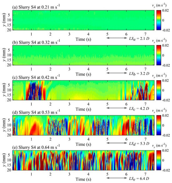
Figure 35.
Images of the radial velocity component as a function of time showing the intermittent structures observed during transitional flow for the cross-sectional plane of a slurry (of density kg m−3) formed with a concentration of clay particles in water of 17%, using ultrasound imaging velocimetry. In each plot, indicates the length scale in terms of the pipe diameter D. Figure taken from Thota Radhakrishnan et al. [370].
Laser-Doppler anemometer measurements of components of the Reynolds stress tensor in turbulent pipe and channel flow of non-Newtonian fluids were reported by Allan et al. [353] and Willmarth et al. [354]. Their findings confirmed that very dilute polymers can produce damping of the radial and cross-flow normal stresses and amplification of the axial normal stress close to the conduit walls. Later experiments were conducted by Pinho and Whitelaw [355] in a fully developed pipe flow with four concentrations of sodium carboxymethyl cellulose in aqueous solution. They also confirmed a delay in the flow transition to turbulence possibly caused by shear-thinning. For a solution of sodium carboxymethyl cellulose 0.2 wt%, turbulence was not seen below 10,000, while for a polymer solution 0.4 wt%, turbulence could not be achieved in their experimental rig.
The pressure distribution along a square-sectioned pipe was experimentally measured for a non-Newtonian pseudo-plastic () fluid flow by Salem and Embaby [375]. They used as a working fluid a water solution of sodium carboxymethyl starch. The results indicate that under laminar and turbulent flow conditions, the pressure distribution is not linear in the pipe entrance zone, and the pressure drop along the pipe increases with increasing polymer concentration and/or flow rate. They also reported a transitional and an increase in the entrance length with increasing power-law index n and/or flow rate. In a more recent work, Haldenwang et al. [376] predicted pressure gradients for the flow of sludge in pipes with different concentrations of sludge and pipe diameters. The Bingham plastic rheological model was used to characterize the flow behavior of sludges with concentrations between 3.4 and 7.2%. They found that the F- correlations that resulted in the most accurate prediction of the pressure loss associated with the flow of sludges for the concentrations and pipe diameters considered were those based on definitions (53) and (61) of the generalized Reynolds number.
It is well known that erosion, corrosion and scale can give rise to pipe roughnesses, which, in general, can be larger than is actually accounted for in the Moody diagram [377]. Friction factor correlations designed to describe the transition from smooth to fully rough pipes for turbulent pseudo-plastic fluids were developed by Kawase et al. [378], while Slatter [374] also investigated the effects of pipe roughness on the pipe flow of Herschel–Bulkley fluids. Later experiments on the behavior of non-Newtonian fluids in rough-walled pipes were conducted by Slatter and van Sittert [379], who found that for graded sand in pipes of 28 and 46 mm internal diameter, the laminar flow region was unaffected by the pipe roughness in agreement with early experimental findings of Nikuradse [34] that the laminar flow regime is not sensitive to the pipe roughness. Slatter and van Sittert also found for pipes with different roughnesses and same size that the turbulent flow always started at the same pseudo-shear rate. A more recent experimental investigation of the effects of large roughness on the pipe flow of slurry was provided by Graham et al. [377]. They used test fluids composed of 0.09, 0.13 and 0.15% Carbopol in water to produce yield viscoplastic fluids with differing rheologies. In addition, 9 and 11% bentonite suspensions in water were also employed as alternative non-Newtonian fluids. They confirmed insensitivity of the laminar flow to the texture or granularity of the pipe roughness and found that for all fluids tested, the laminar flow regime can be accurately predicted by using a constricted pipe diameter.
In order to minimize sedimentation of particles in the bottom side of a pipe during mud slurry flow in horizontal pipes, Yanuar et al. [380] performed experiments of mud slurry flow in spiral conduits as shown in the top image of Figure 36. Slurries with mud particle concentrations of 20, 30 and 40% were tested at isothermal conditions at a temperature of 27 °C. The plots in the lower part of Figure 36 depict the F- relationship obtained experimentally for the laminar and turbulent flow of each working fluid in the circular (see Figure 36a) and spiral pipe with a ratio of the pitch to outside diameter (see Figure 36b). The experimental data are compared with the Hagen–Poiseuille equation for the laminar flow and the Blasius equation for the turbulent flow. At large , the flow in the spiral pipe shows a more significant decrease in the friction factor below the Blasius equation compared to the circular pipe, which becomes even more significant when is increased to 7.3 (see Yanuar et al.’s [380] Figure 6). However, for the laminar flow, there is no decrease in the friction factor below the Hagen–Poiseuille flow regardless of the pipe geometry and fluid rheology. Evidently, these results show that the efficiency of slurry flow increases in spiral pipes, which is a need in many industrial processes, including, for example, the flow of mud during drilling operations [381].
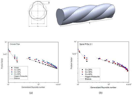
Figure 36.
(Top) Geometry of a spiral pipe. (Bottom) Darcy–Weisbach friction factor as a function of the generalized Reynolds number, as given by Equation (57) with and , for (a) a circular pipe and (b) a spiral pipe with , where P is the pitch and is the outside diameter. Figures taken from Yanuar et al. [380].
Although experimental research on non-Newtonian fluid flow in pipes has been very active in the last 30 years, there are still several aspects that remain underexplored or inadequately addressed. For example, non-Newtonian fluids, particularly those exhibiting shear-thinning or viscoelastic properties, experience transition to turbulence at lower Re values compared to Newtonian fluids. This transition is often characterized by weak turbulence with a rather chaotic time dependence and regular spatial structures. Understanding these instabilities is of fundamental importance for accurate prediction of flow behavior in real applications. On the other hand, more experimental studies are clearly needed to understand the influence of pipe roughness on non-Newtonian fluid flows. Difficulties in obtaining accurate measurements of velocity profiles and rheological properties impose an additional barrier to achieving a full understanding of non-Newtonian fluid transport in pipeline systems. Addressing these gaps through targeted experiments will certainly enhance the level of prediction of numerical models and improve both the design and operation of systems involving non-Newtonian fluid flow in pipes.
6.4. Numerical Simulations
Pipe flow simulations of power-law fluids began to appear in the literature between the late 1990s and the early 2000s, long after the first numerical simulations of Newtonian pipe flows. Since these flows occur in a wide range of industrial processes, their simulations have grown in number over the last 20 years. Of greatest interest are transitional and turbulent flows. However, if the flowing fluid has a high yield stress, or if its effective viscosity is high, flow rates in the laminar regime will certainly be of more interest for the industry.
LES of turbulent flow of a non-Newtonian fluid in channels were first reported by Blackburn [382] using SEM, while Beris and Dimitropoulos [383] used pseud-spectral methods to perform a DNS of the flow of viscoelastic fluids in a channel. However, the lack of mesh refinement in these latter simulations introduced small errors which had the artificial effect of lowering the drag reduction capability of the simulated fluid. Later, Rudman et al. [384,385] presented DNS of weakly turbulent, transitional and turbulent pipe flows of power-law fluids. Their numerical results predicted profiles of the superficial velocity having a different shape compared to the experimental data of 0.5 wt% carboxymethyl cellulose in aqueous solution by Escudier and Presti [366]. In addition, the predicted values of the velocities were found to be lower than indicated by the experiments. At the time, this discrepancy was indicative of the difficulty of modeling real polymer solutions with power-law fluid models in that the elastic and elongational effects that influence the experiments were not accounted for in the simulations. Rudman and Blackburn [386] performed further DNS of turbulent pipe flows of power-law thinning fluids using a spectral element-Fourier formulation of the Navier–Stokes equations. Their results were found to agree qualitatively well with the logarithmic layer correlations determined experimentally by Clapp [387] and suggested that the generalized Reynolds number at which transition occurs increases with decreasing power law index and increasing deviation from Newtonian rheology. They also noted that the transition to turbulence for , 0.69 and 0.73 occurs through a multistep process between intermittent (i.e., puffs and slugs) and turbulent events as was recently observed experimentally by Thota Radhakrishnan et al. [370] for transitional non-Newtonian pipe flow.
Yao et al. [388] studied the fully developed flow of a pseudo-plastic fluid through a circular pipe using a one-dimensional, four-parameter model based on the two-parameter Ostwald-de Waele power law [389]. The proposed model was designed to represent the lower and upper regions of the Newtonian behavior characteristic of pseudo-plastic polymer melts and solutions, while the model parameters were determined to fit available experimental data for the variation of the non-Newtonian viscosity of a 0.4% polyacrylamide solution with shear rate. The resulting balance momentum equation with a shear-rate-dependent viscosity was integrated using the trapezoidal rule. It was found that at low values of the shear-rate parameter, the velocity predicted by the modified model is higher than that predicted by the power law, while the converse occurs at high values of the shear-rate. However, at intermediate values, the predicted velocities were found to be similar for both models. In passing, we note that Tozzi and Hartt [390] have recently proposed a method to convert velocimetry experimental data to a curve of flow rate versus pressure drop without the need of fitting the data to any rheological models (i.e., constitutive equation). On the other hand, Radulescu and Radulescu [391] have investigated the flow of power-law () fluids in a circular pipe with slip boundary conditions, finding that both the power-law index and the dimensionless slip coefficient may influence the streamwise velocity profile. A fully implicit SPH method for the simulation of highly viscous fluid flows was recently developed by Morikawa et al. [392], who applied it to the exploratory simulation of the flow of a Bingham plastic fluid through a straight pipe of circular cross-section. They obtained excellent results when compared with the theoretical value of the pipe flow velocity developed by Mattiusi [393].
It is well known that sudden changes in the flow rate caused, for example, by valve closure and pump operations in pipeline systems, can lead to significant pressure oscillations in the flow, which in turn may lead to devastating forces with a consequent damage to the pipeline [394]. This phenomenon is commonly known as water (or fluid) hammer. The interested reader in learning more about this phenomenon is referred to the paper by Ghidaoui et al. [395] (and references therein), where the theory and practice of water hammer are thoroughly reviewed. Two-dimensional analyses and simulations of the water hammer phenomenon in pipeline systems have been performed by several scholars [396,397,398,399,400,401,402,403,404,405,406,407,408]. In particular, Pezzinga et al. [405] reported an interesting analysis of transients in pressurized polymeric pipes using a two-dimensional Kelvin–Voigt viscoelastic model. They found that pressure oscillations and velocities decay faster in viscoelastic models owing to a time lag between the pressure oscillations and the retarded circumferential strain. Power-law and Cross fluid models were later considered by Majd et al. [408] to simulate the transient non-Newtonian pipe flow associated with water hammer in a reservoir–pipe–valve system, using FD methods to represent the unsteady flow equations and a fourth-order Runge–Kutta scheme for their time integration. An example of the pressure oscillations at the valve and midpoint of the pipe is shown in Figure 37 for a highly viscous oil ( N s m−2) under laminar flow conditions at and measured wave velocity equal to 1324 m s−1. Majd et al. [408] found that the pipe flow of pseudo-plastic liquids with greater shear-thinning properties shows a reduced pressure drop over time. This occurs due to a reduction in the apparent viscosity at the wall, which in turn causes a reduced line-packing effect compared to pure Newtonian fluid flows. In addition, the shear-thinning behavior of the flowing fluid causes high velocity gradients to concentrate near the pipe wall, thereby leading to severe fluctuations in the cross-sectional velocity profiles.
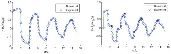
Figure 37.
Pressure signals directly upstream of the valve (left) and at the pipe midpoint (right) caused by a sudden valve closure in the laminar pipe flow of a highly viscous oil. The simulation results (symbols) are compared with experimental data (solid lines) [409]. Figures taken from Majd et al. [408].
Although numerous experimental and numerical studies of Newtonian fluids in smooth and rough pipes can be found in the literature, only a limited number of investigations are available for non-Newtonian fluids flowing through rough-walled pipes. Recently, Sorgun et al. [410] performed CFD calculations of turbulent flow of Herschel–Bulkley and power-law fluids in rough pipes. The numerically obtained results for the frictional pressure gradient were compared with their own experimental data for three different pipe diameters (, 80 and 90 mm) and roughness heights (, 0.07 and 0.12 mm). The experiments were conducted with two highly viscous, non-Newtonian fluids consisting of carboxymethyl cellulose polymers with different weights, which were numerically mimicked by a power-law fluid with no yield point and a Herschel–Bulkley fluid. In all cases, the computed frictional pressure gradient agrees reasonably well with the experimental data for the range of values considered. However, a comparison with Reed and Pilehvari’s [411] friction factor equation shows that it overestimates the pressure gradient. In most cases, their predicted pressure gradient can reproduce the experimental data within an error of %.
Following a different approach, Bouchendouka et al. [412] reported a fractal analysis of the flow of power-law fluids (covering shear-thinning, Newtonian and shear-thickening behavior) in a rough pipe.
In these models, the roughness of the pipe is considered to be fractal (see Figure 38). The circular perimeter of the pipe is related to its cross-sectional area by the relation , where is the fractal dimension (). For a smooth surface , while when , the surface becomes fractal. Defining as the average pipe radius, then . In three dimensions, the roughness of a pipe can be described by the surface fractal dimension and the surface area , where is the volume enclosed by the pipe surface and L is its length. Here, , where represents a perfectly smooth surface, and describes a fractal pipe surface. The influence of the surface fractal dimension on the streamwise velocity profile for varying values of the power-law index n is shown in Figure 39. In general, the value of does not modify the shape of the velocity profile but only its amplitude. However, the amplitude is seen to decrease with increasing , which is expected since is a measure of the surface roughness. Therefore, the friction losses increase accordingly. The decrease in the amplitude with increasing is observed to be faster for shear-thinning () fluids compared with Newtonian () and shear-thickening () fluids, implying that pseudo-plastic fluids are more sensitive to the surface roughness. Figure 9 of Bouchendouka et al. [412] depicts the friction factor as a function of for , 10, 20, 30, 40 and 50 Pa. For , the friction factor increases with increasing for all values of , while for , it decreases with increasing . An interesting feature of the results is that for , there is always a critical value for which the friction factor is approximately the same regardless of the value of n. This critical value is strongly dependent on the pressure difference as it increases with increasing .
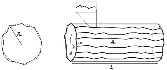
Figure 38.
(Left) Schematic of a fractal cross-section. (Right) Schematic of a fractally structured pipe wall surface. Figures taken from Bouchendouka et al. [412].
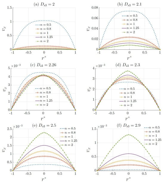
Figure 39.
Streamwise velocity profiles for different surface fractal dimensions and values of the power-law index n. Here, , mm and the pressure gradient is equal to 5 Pa. Figure taken from Bouchendouka et al. [412].
The steady flow of a Herschel–Bulkley fluid in a square-sectioned conduit with a sudden expansion was studied numerically by Alexandrou et al. [413], using a mixed-Galerkin finite element formulation coupled with a Newton–Raphson iteration procedure. Flow details were obtained for 2:1 and 4:1 expansion ratios. A recirculation zone forms in the corner of the sudden expansion, whose size increases with increasing generalized Reynolds number and expansion ratio. Their results also revealed a strong interplay between and the generalized Bingham number
where is the yield stress, H is half the height of the inlet cross-section, v is a characteristic mean velocity, K is the consistency index, n is the power-law index and is the effective viscosity with being the shear rate. The value of was found to influence the size and shape of the unyielded zone just behind the expansion, which increases with increasing . However, the effects of are more pronounced for small values of due to the interplay between inertia, viscous and finite-yield effects. Xu et al. [414] introduced a SPH formulation for studying the flow of non-Newtonian fluids in pipes and in free-surface flow problems. Using the rheological Cross model for the viscosity, they simulated the Hagen–Poiseuille flow in a cylindrical pipe and the fluid injection molding of a Z-shaped mold. The same approach was also applied to study the transient behavior of two-dimensional viscoelastic flows using Brownian configuration fields [415]. Accurate results for plane Poiseuille flow for a Hookean dumbbell (Oldroyd-B) fluid and a purely elastic upper-convected Maxwell model were obtained.
Numerical simulations of a non-Newtonian fluid flow in a long straight circular pipe including an obstacle were performed by Yavuz and Sari Çavdar [416] for power-law indices , 0.5, 1 and 2. A circular obstacle attached to the wall of the pipe was placed at a distance of from the inlet. The results show that a dead flow zone is produced in front and rear of the obstacle and that the axial flow velocity increases as it passes the obstacle due to the narrowing. The profiles look quite asymmetric with a sharper and higher parabolic curve for . As the flow leaves the obstacle region, the flow asymmetry decreases and eventually stabilizes and returns to a symmetrical distribution at from the inlet.
Glass production involves transporting the glass melt through pipes and ducts that connect the melting furnace with the forming device, where the melt is cooled down to a suitable forming temperature. During the cooling process, the physical properties of the melt, including its viscosity, change sharply, leading to unwanted inhomogeneities in the final glass product. Therefore, numerical simulations aimed at predicting pipe flow under temperature-dependent fluid properties have become necessary. For example, Wylie and Lister [417] performed a linear stability analysis to two- and three-dimensional disturbances of the pressure-driven flow of an initially hot viscous fluid through a planar channel with cold walls. For large viscosity changes due to cooling from the sidewalls and certain values of the fixed pressure drop, they predicted three different two-dimensional steady-state solutions. When three-dimensional disturbances are considered, the flow becomes unstable to fingering instabilities. A linear stablity analysis of pipe flow of glass melts by Lange and Loch [418] yielded similar results. An important conclusion from these linear stability analyses is that under a temperature-dependent viscosity, the characteristics of laminar flow can be dramatically modified. Giessler et al. [419] presented two-dimensional axisymmetric simulations of the laminar and steady flow of a glass melt through a circular pipe driven by a pressure difference, using the commercial software COMSOL. The highly viscous fluid was assumed to have strongly temperature-dependent viscosity and electrical conductivity, and it was heated by internal electromagnetic Joule heating and cooled by the pipe wall by convection. Figure 40 shows the mean flow velocity as a function of the applied pressure gradient for different values of the constant thermal conductivity, , as compared to the one-dimensional model developed by Giessler et al. [420], describing the nonlinear laminar flow of a highly viscous fluid (glass melt) under the coupled effects of wall heat loss and internal volumetric heating. For intermediate and high values of , the mean velocity and pipe outlet temperature are in good agreement with the predictions of the one-dimensional model. However, for small thermal conductivities ( W m−1 K−1), the numerical results deviate from the predictions of the one-dimensional model. A bifurcation exists in the one-dimensional model (see also Giessler et al.’s [419] Figures 3–11), which is absent in the results of the two-dimensional simulations.
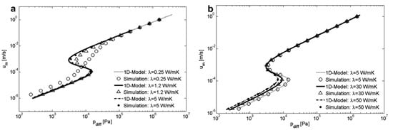
Figure 40.
Mean flow velocity as a function of the applied pressure difference for the flow of glass melt through a circular pipe as compared with the predictions of the one-dimensional model developed by Giessler et al. [420] for varying thermal conductivities: (a) λ = 0.25 W m−1 K−1, 1.2 W m−1 K−1 and 5 W m−1 K−1 and (b) 5 W m−1 K−1, 30 W m−1 K−1 and 50 W m−1 K−1. Figures taken from Giessler et al. [419].
Recently, Fernandes et al. [421] reported numerical simulations of the flow of polymer melts obeying the Herschel–Bulkley constitutive equation, using a new scheme based on the Arbitrary Lagrangian–Eulerian (ALE) formulation. Their method was validated against the extrudate swell ratio of shear-thinning and shear-thickening data previously reported by Kountouriotis et al. [422]. Figure 41 shows the dependence of the extrudate swell ratio, , on the Bingham number for power-law fluids with and 1.5 at , 5 and 10. The solid lines correspond to the results obtained by Kountouriotis et al. [422]. In general, the values of for shear-thinning () are always lower than those for shear-thickening () behavior. As increases, the die swell ratio decreases similarly to the extrudate swell observed for a Newtonian fluid [423]. In addition, for the Herschel–Bulkley flows of the shear-thinning fluid, the value of was observed to vary by about 8% from to 10 when the effects of the yield stress are negligible (i.e., Bingham number equal to 0.001). However, at higher values of the Bingham number, the effects of the yield stress dominate and , implying that the polymer melt neither contracts nor expands.
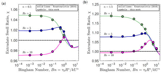
Figure 41.
Extrudate swell ratio, , as a function of the Bingham number for the isothermal extrudate swell of Herschel–Bulkley fluids at , 5 and 10 for (a) (shear-thinning behavior) and (b) (shear-thickening behavior). Figures taken from Fernandes et al. [421]. The solid lines correspond to the results obtained by Kountouriotis et al. [422].
Numerical simulations come with a number of limitations due to the complex nature of non-Newtonian fluids and the lack of accurate experimental measurements. The reliability of numerical model results can be compromised by the fact that non-Newtonian fluid behavior requires complex constitutive equations, which, in turn, are difficult to calibrate and validate. Moreover, the accurate modeling of such flows requires high spatial resolution and smaller time steps, leading to large computational demands. Other drawbacks can be associated to convergence and stability issues, the requirement of wall-slip boundary conditions for some non-Newtonian fluid flows and oversimplification of secondary effects like, for example, temperature dependence, phase change and elastic instabilities in viscoelastic fluids.
7. Entropy Generation in Pipe Flows
In the fluid flow through a pipe, the irreversibility, as in any other thermodynamic system, is, in general, related to energy dissipation by viscous friction and heat transfer. According to the second law of thermodynamics, the entropy of the system increases when an irreversible process takes place. As entropy increases, energy becomes less and less available to do work. Therefore, the minimization of entropy generation, also called thermodynamic optimization in engineering, is necessary to provide an efficient use of the available energy [424]. In other words, the loss of available energy due to dissipation by fluid friction and heat transfer is responsible for the irreversibilities, which, in turn, are quantified in terms of the production of entropy. In particular, energy dissipation by heat transfer caused by a finite-temperature gradient characterizes heat transfer processes by convective motions in the fluid.
Nag and Kumar [425] performed a second-law analysis of heat transfer due to convective motions in a fluid that flows through a conduit with constant heat flux. They expressed the rate of entropy production in terms of the temperature difference between the fluid and the wall and the frictional pressure drop and found the value of the temperature difference for which the entropy generated is a minimum. However, in this case, the product of the Stanton number, defined by
where is the convective heat transfer coefficient and is the specific heat capacity, and the temperature difference does not vary due to the constant heat flux imposed on the pipe. Therefore, in order to provide a more accurate determination of the entropy production, Şahin [426] performed a similar thermodynamic analysis to account for the effects of a temperature-dependent fluid viscosity in the laminar flow through a cylindrical pipe subjected to constant heating. Starting from the total heat flux
and the entropy generation within a volume control
where is the mass flow rate, and is the pipe wall temperature, Şahin [426] obtained the following expression for the dimensionless entropy generation
where , , is the dimensionless temperature difference between the wall and the bulk flow, is the dimensionless length of the pipe, is the fluid temperature at the pipe inlet and is the Eckert number, defined by
For low viscosity , and the second term between brackets in Equation (75) can be neglected. If the empirical correlation for the temperature-dependent viscosity of liquids [427]
where m and B are fluid-specific parameters, is used, then the total entropy generation becomes
where the integration along the full length of the pipe must be performed numerically. According to Equations (75) and (78), the entropy generation is a function of three dimensionless numbers, namely, , and . In addition, since increases along the pipe, no optimum length can be obtained for a constant viscosity. However, an optimum pipe length can be obtained, which minimizes the energy loss due to both entropy generation and pumping power, while for low heating fluxes (i.e., for ), entropy production is due primarily to viscous friction. For fully developed laminar flow, Şahin [428] performed a thermal effectiveness analysis with the aim of optimizing the design of a heat recuperator when viscous frictional heating is included, finding that the optimum size for which thermal effectiveness becomes a maximum depends on the viscosity of the flowing fluid.
Şahin [429] also investigated by analytical means the entropy generation of a fully developed laminar flow of a viscous fluid through a cylindrical pipe under the effects of a constant wall temperature. It was found that when the temperature difference between the inlet fluid and the wall rises, the entropy generation increases. However, since the pumping power decreases with increasing temperature difference, a value of the fluid inlet temperature exists for which the exergy loss is minimum, a result which is valid for both constant and temperature-dependent fluid viscosities. Following a similar analysis, Şahin [430] derived an analytically counterpart expression for the entropy generation for turbulent liquid flow in a cylindrical pipe subjected to a constant wall temperature. In general, heat transfer to the fluid occurs through a mean heat transfer coefficient, , which is a function of the viscosity variation. Using the form of given by Kays and Crawford [431], namely, , where is a constant property average heat transfer coefficient, given by
and are, respectively, the fluid viscosity at the bulk and wall temperature, for heating and 0.25 for cooling and F is the average Darcy–Weisbach friction factor for a smooth duct flow with a temperature-dependent viscosity [432]
Şahin [430] obtained the following expression for the entropy generation, which for the assumption of a constant viscosity obeys the expression
where now and . Figure 42 shows the dependence of the entropy generation on the inlet temperature difference, , for water and glycerol turbulent flow when the fluid viscosity is assumed constant, linearly dependent on the temperature and given by Equation (77) (corresponding to Şahin’s [430] Equation (2)). Since the viscosity of water is relatively low, the entropy generation is the same for a constant, linear and variable viscosity model, while the effects of the viscosity model are more evident for glycerol, where the minimization of the entropy production for values of is larger when a variable viscosity is assumed. At values of lower than 0.1, the total energy production is dominated by frictional effects. Narusawa [433] investigated the rate of entropy production for forced and mixed convection in fully developed flow in a rectangular channel heated from below.
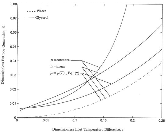
Figure 42.
Entropy generation as a function of the temperature difference between the inlet fluid and the pipe wall for the turbulent flow of water and glycerol through a cylindrical pipe subjected to a constant wall temperature. Equation (2) in the figure corresponds to the viscosity dependence on temperature given by Equation (77), while corresponds to in our notation for the shear viscosity. Figure taken from Şahin et al. [430].
Investigations of entropy generation in non-Newtonian pipe flow date back no more than 15 years. However, Mahmud and Fraser [434] reported an early second law analysis to study inherent irreversibilities in the flow of a non-Newtonian fluid through channels and pipes. More recently, Bouzid et al. [435] studied the entropy generation in a fully developed laminar flow of ice slurry under the effects of a uniform heat flux at the pipe wall. They modeled the ice slurry as a non-Newtonian fluid obeying a power-law model with the index n depending on the mass fraction of ice, , as
for . They obtained an analytical solution for the average volumetric entropy generation in terms of n, the temperature difference, the Péclet number () and the Brinkman number, defined as
where is the reference temperature difference, q is the wall heat flux and D is the pipe diameter. They found that as the mass fraction of ice in the slurry increases the entropy production also increases, while the minimization of the entropy production is observed only when for and (see their Figure 4), where is the temperature of the ice slurry at the pipe inlet. Based on the Herschel–Bulkley rheology model, Pan et al. [436] studied both theoretically and experimentally the flow of lubricating grease in a pipe. Experimentally, it was observed that at high temperatures, the flow rate weakens as a result of the correspondingly low yield stress. On the theoretical side, these scholars found that the flow rate increases with pipe diameter and pressure gradient, the effects becoming more evident at high temperatures.
In more recent work, Mondal and Wonwises [437] studied the entropy generation of a Newtonian fluid flow through a narrow annular conduit between two asymmetrically heated concentric cylinders, where the inner cylinder was rotating at a uniform rate. In this case, the volumetric entropy production rate obeys the relation
where is the initial fluid temperature, r is a radial coordinate and is the viscous dissipation term. It was observed that heat transfer in the fluid layer surrounding the wall of the rotating inner cylinder is reduced due to enhanced viscous heating there. For , the entropy production rate is reduced close to the inner cylinder, while for , the opposite occurs in that the heat transfer rate is higher in the region near the inner cylinder, thereby leading to higher entropy generation there. As a final remark in this section, it is worth commenting on the very recent experimental work of Jo et al. [438], who measured the viscosity of non-Newtonian fluids (that is, Xanthan gum solution and drilling mud) in complex pipe systems based on energy dissipation rates. For flow through a straight pipe with connectors, a pipe system with an intermediate branch and a pipe system with slope and height variations, the accuracy of the viscosity measurements and pressure drop prediction was within an error of 18.7% in all cases considered.
8. Hydromagnetic Pipe Flows
The flow of electrically conducting liquids in the presence of magnetic fields has also gained special attention because of its frequent occurrence in many industrial applications. These flows are also referred to in the literature as hydromagnetic flows. Of particular technical importance is the laminar flow of such liquids in a pipe under the effects of a uniform magnetic field because of the use of induction flow-meters with liquid metals. The first studies of hydromagnetic pipe flows date back to 1937 with the work of Hartmann [439], who found an exact solution for the flow between two infinite parallel non-conducting plates for the case when the magnetic field is applied perpendicular to the plates. Later, Shercliff [440,441,442] presented solutions for the more general problem of hydromagnetic flows in a rectangular channel and in straight pipes of circular cross-section with non-conducting walls. He showed that for large values of the Hartmann number
where B is the intensity of the magnetic field, l is a characteristic length scale (i.e., the width of a channel or the diameter of a circular pipe) and is the electrical conductivity, the axial flow velocity profile degenerates into a uniform core surrounded by boundary layers near the walls. The Hartmann number quantifies the importance of electromagnetic forces over viscous forces. Shercliff [441] estimated the entrance length over which the laminar motion of an electrically conducting, viscous fluid in a pipe under a transverse magnetic field becomes stationary.
Chopra [443] also studied the flow of an electrically conducting liquid in a circular pipe under a transverse uniform magnetic field, predicting that the axial velocity profile gradually changes from a parabolic shape to a plateau as the strength of the applied magnetic field is increased. Although these findings comply with earlier results obtained by Hartmann [439], Chopra [443] suggested that the transition from a parabolic profile to essentially a plateau is due to the viscosity being dominant near the pipe wall and the induction drag working more efficiently in the central layers when the intensity of the magnetic field increases. For the same flow problem, Gold [444] derived an exact solution valid for all values of , which was in good agreement with the experimental results for the flow of mercury in circular and rectangular pipes reported by Hartmann and Lazarus [445] for low-to-intermediate values. Singh [446] performed a theoretical analysis of steady motion of a conducting fluid in a curved pipe and observed the formation of Dean vortices only when the magnetic field is dropped. Later, Vidyanidhi and Ramana Rao [447] carried out a theoretical analysis of the hydromagnetic flow of a viscous incompressible fluid along a straight circular pipe with a constant pressure gradient and rotating about an axis perpendicular to its elongation. In particular, they studied the case of small angular velocity and . Their solution consisted of successive approximations in ascending powers of , where the first approximation corresponds to . In this case, a secondary flow sets in similar to the spiral fluid motion along the pipe described by Barua [448] for a non-magnetic viscous fluid flow. Gupta [449] studied the unsteady flow of an electrically conducting viscous fluid in a circular pipe of non-conducting wall under the influence of a uniform transverse magnetic field, finding that for small values of , the flow velocity near the pipe center increases more rapidly than for the case of a non-conductive fluid ().
The feasibility of a magnetic field to prevent the transition from laminar to turbulent flow in an electrically conducting fluid was studied experimentally by Fraim and Heiser [450]. They used mercury as the working fluid and a magnetic field in the streamwise flow direction, finding that the transition to turbulence was considerably delayed to a much larger than for a non-conductive fluid. Whereas in the presence of a transverse magnetic field the mean axial velocity profiles are modified, the same is not true in presence of longitudinal magnetic fields. For example, the stability analysis performed by Nachtsheim and Reshotko [451] shows that the flow is largely stabilized for a combination of low magnetic Reynolds numbers
and large Alfvén numbers
so that the interaction parameter remains finite, where is the magnetic permeability, B is the intensity of the applied longitudinal magnetic field, v is the mean centerline flow velocity and R is the pipe radius. However, for large , the flow becomes unstable. This is not the case in typical experiments of liquid metal pipe flows where the values of are rather small. Such flows can only be destabilized under the action of very intense magnetic fields.
It must be noticed that all references cited above deal with early work from 1937 to 1968 when many studies on hydromagnetic pipe flows were indeed published. From 1968 until the mid-90s, there was a shortage of work on hydromagnetic pipe flows. Exceptions to this rule are given by McMichael and Deutsch [452], who have considered the perturbation of Poiseuille flow by the application of a longitudinal magnetic field with a weak axial gradient for small and finite and , and by D’Arcy and Schmidt [453], who analyzed the development of the velocity profile for flow at the entrance of a channel in the presence of a longitudinal magnetic field. These latter authors found that the presence of the magnetic field retards the development of the velocity profile by producing Lorentz forces, which oppose the movement of fluid from the viscous wall region to the core. It was not until 1995, when Åkerstedt [454] reported on the stability of three-dimensional disturbances in the pipe flow of an electrically conducting fluid in the presence of a longitudinal magnetic field. Their results indicate that substantial hydromagnetic damping of the transient energy growth occurs for short wave perturbations and moderate values of the interaction parameter, I, between approximately 1 and 3, while for longer waves, the magnetic field perturbations decouple from the flow and, therefore, have no effect on destabilizing the flow.
Hydromagnetic flow separation in a diverging channel in the presence of an externally applied homogeneous magnetic field was further studied by Makinde and Mhone [455], using perturbation methods and a Padé approximation technique for solving the governing hydromagnetic flow equations. They found that internal flow separation is observed at low values in the range , with increasing with increasing intensity of the magnetic field, while at higher , flow separation is suppressed or even prevented at all when the intensity of the applied magnetic field is further increased. These results were much later confirmed by Mallik et al. [456], who employed a similar solution formalism to study flow separation in a linearly diverging channel in an externally applied uniform magnetic field.
More recently, Gedik [457] carried out experimental and numerical investigations of the flow of magneto-rheological fluids in a circular pipe in the presence of a uniform magnetic field. Previous work of magneto-rheological pipe flows dates back to 2009, and, for more details, the interested reader is referred to the references cited in Gedik’s [457] paper. The experiments were carried out to study the effects of varying the magnetic field intensity between 0.01 and 0.15 T on the laminar flow of three different magneto-rheological fluids in long pipes of 10 and 15 mm diameter. The fluid samples consisted of 20% (Fluid A), 15% (Fluid B) and 10% (Fluid C) concentrations of BASONETIC 5030-4035-2040 fluids diluted in a poly--olefin solution doped with magnetizable carbonyl iron powder. The physical properties of each of these fluids were copied for use in CFD simulations using the ANSYS Fluent 14.0 solver. The numerical simulations were found to reproduce with good accuracy the experimental measurements. In particular, as the intensity of the magnetic field is increased, the fluid viscosity increases, and consequently the flow velocity decreases. However, the flow velocities are higher in the 10 mm than in the 15 mm pipe diameter. Figure 43 shows the experimental and numerical values of the flow velocity as a function of for both pipe diameters and all fluids and magnetic field intensities considered. The deviations between the numerical results and the experimental data were found to be all within 2.5%.
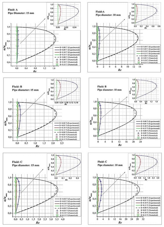
Figure 43.
Experimental and numerical axial flow velocity as a function of the Reynolds number of a magneto-rheological fluid in a straight pipe of circular cross-section under the influence of an externally applied transverse magnetic field. The plots show the axial velocity for three different electrically conducting fluids, two pipe diameters and varying magnetic field intensities. Figure taken from Gedik [457].
Nagaraju and Garvandha [458] performed an analytical investigation of an axisymmetric incompressible viscous fluid flow in a circular pipe under the effects of suction/ejection over the pipe wall and a constant magnetic field opposite to the wall. It was found that as the magnetic force and the suction Reynolds number are increased, the axial flow decelerates and the radial flow accelerates. In addition, the temperature increases with an increasing Prandtl number and decreases with an increasing Eckert number as a result of viscous dissipation effects. Nkengmene et al. [459] investigated the hydromagnetic instability of the isothermal flow of an incompressible viscous fluid in a cylindrical rotating pipe subjected to a uniform magnetic field by means of a linear stability analysis and numerical simulations based on a divergence-free Petrov–Galerkin approximation of the magnetohydrodynamic equations. It was found that for small pipe rotations and weak magnetic fields, the flow exhibits some unstable modes that can induce three-dimensional perturbations, while the flow stabilizes for large pipe rotations. In a very recent work, Velizhanina and Knaepen [460] performed a linear stability analysis of a fully developed liquid–metal hydromagnetic pipe flow in the presence of a transverse magnetic field. Due to the asymmetry in the axial flow velocity profile, the numerical solution was based on a two-dimensional complex eigenvalue solver relying on a Chebyshev–Fourier collocation method. In contrast to the linear stability exhibited by the Hagen–Poiseuille flow at all values, the analysis revealed that hydromagnetic pipe flow under the action of a transverse magnetic field is unstable to three-dimensional perturbations at high values and wall electrical conductance ratios. A major finding of Velizhanina and Knaepen’s [460] analysis is that a global Reynolds number for the hydromagnetic flow with transverse magnetic field is = 45,320, which was observed to occur for a perfectly conducting pipe wall and .
Recent numerical simulations of hydromagnetic flow of a non-Newtonian, shear-thickening fluid through a convergent conduit in the presence of a variable transverse magnetic field were reported by Wawira et al. [461]. In their numerical solution scheme, the nonlinear governing equations are reduced to a system of ordinary differential equations, which are solved numerically by a collocation method in MATLAB bvp4c. The results indicate that the flow velocity, temperature and magnetic induction are higher at the pipe centerline because there the retarding effects of viscosity are smaller. In addition, all these flow properties are observed to increase with increasing Reynolds number, Hartmann number, Eckert number and Joule heating parameter. On the other hand, at high values, the convective heat transfer and the fluid velocity decrease, confirming previous findings. Therefore, it was concluded that while a less viscous fluid facilitates the pipe flow, the presence of a strong magnetic field works in the direction of reducing the fluid motion.
The study of the pipe flow of liquid metals under the action of an external magnetic field introduces unique challenges beyond fluid dynamics: first, because consistent numerical simulations require combining the Navier–Stokes equations with Maxwell’s equations for the electromagnetic field and, second, due to the lack of experimental measurements for model validation. Experimental work on this type of flow requires the use of non-conductive or insulated pipe walls to avoid induced currents or even short-circuiting without losing sight of the fact that electromagnetic forces can cause excessive heating, corrosion and eventually material fatigue. These difficulties explain the scarcity of experimental data, which limits the validation of numerical models. Moreover, working with strong magnets to maintain a strong, uniform magnetic field over long pipes is both energy-intensive and technically challenging. In addition, the density and viscosity of liquid metals change as a result of Joule heating, while nonlinear thermal effects arise as a result of temperature-dependent conductivity. Therefore, future research in this line must focus on innovative experimental designs and reliable numerical models that validate the available experimental data.
9. Pipe Flow Studies Using Machine Learning and Artificial Intelligence
9.1. Machine Learning
Machine learning (ML) applications in computer science have gained increasing ground in the last few years. In particular, ML modeling is constantly used to enhance and speed up standard CFD simulations, increasing their accuracy and efficiency. In addition, it provides room for more complex analysis as ML algorithms can be used to learn patterns from large experimental and numerical data sets and produce data-driven models that capture the behavior of complex flows with considerably much lower computational costs. The importance of enhancing traditional standard fluid-flow solvers by introducing ML techniques, relying on multilayer perceptron neural networks combined with Principal Component Analysis transformations, has recently been addressed by Sousa et al. [462]. A conventional approach involves training ML models with flow fields generated by numerical solutions of the continuity and Navier–Stokes equations. The flow simulations can be enhanced to achieve applicability to any geometry and type of boundary conditions.
ML modeling of pipe flows has mainly focused on two-phase flows for applications to the chemical, nuclear and oil industries [463,464,465]. However, a discussion on two-phase and multiphase pipe flow simulations using ML techniques will be considered in an upcoming review paper in this series. ML models have also been proposed for simulations of natural gas transportation via large-scale pipe networks. For example, Yin et al. [466] have reported a ML-based surrogate model for gas flow control problems in the station-level process piping network. Other recent applications to single-phase pipe flows involve the estimation of water flows in pipeline systems and networks. In particular, Tawfik [467] used an Artificial Neural Network (ANN) to provide accurate solutions of water flow in pipeline systems. The network, consisting of output, hidden and inlet layers with 1, 50 and 2 neurons, respectively, was trained using 90,000 synthetic realizations. After testing this approach for the hydraulic flow discharge of the three tanks problem, the deviation errors between the obtained results and those from an Engineering Equation Solver (EES) software V12.063 were always less than 1.5%. Previously, a similar ANN strategy was used by Brkić and Ćojbašić [468] to estimate friction factor values in pipe flow at and for relative pipe wall roughness between and 0.1. These scholars reported relative errors up to 0.07% compared to explicit accurate approximations of the Colebrook relation. Moreover, ANN was also used to predict pressure losses [469,470] and pressure levels [471] in water supply pipelines. In addition, Dawidowicz [472] reported an estimation of water pipe diameters using ANNs of the multilayer perceptron type, and Roy [473] employed a hybrid ANN method for leak detection in water pipe networks. Leak detection in underground water pipeline systems represents a significant challenge because it is difficult to know the precise status of ducts when excrete or crack occurs, leading to large water losses, increased operational costs and detrimental environmental impacts with a significant affectation to urban infrastructure. In particular, most ANN modules applied as an optimization tool utilize feed-forward-type neural networks, consisting of an input layer, an output layer and single or multiple hidden layers. For instance, Roy [473] used a back propagation algorithm to train the network with generated data against pressure fluctuations in the pipe network, which gave rise to an innovative approach for fluid leak detection in underground hydro-pipe networks.
Pandian and Alphonse [474] have recently proposed to combine CFD simulations and Deep Learning (DL) to enhance the efficiency of leak detection and localization in water distribution systems. They produced a large data set of CFD water flow solutions in pipes of varying diameters and materials by considering different possible leak scenarios. Using these data, they trained and tested two DL models, namely, the Bi-Layered ReLU Encoder + Softmax and the Tri-Layered ReLU Encoder + Softmax, finding improvements in detection accuracy by 2.4% and localization by 5.6%, which shows the potential of this hybrid CFD-DL approach to increase the reliability and efficiency of water management systems. Hayslep et al. [475] employed a data-driven approach by applying linear models, random forests and neural networks to both minimum night flow—a technique used to assess water losses in water distribution networks, which is based on measuring water flow during the night, when consumption in the system is generally low—and pipe failure prediction. In this novel approach, the models were trained to estimate two different measures of historic leakage: average minimum night flows and historic engineering work orders for over 800 real-world district metered areas in the United Kingdom. It was found that both the directly trained models and the leakage contribution score perform well at this task. These results show that modern ML methods can be successfully applied to predict water leak detection and localization due to pipe failure with an ever increasing accuracy and efficiency.
9.2. Artificial Intelligence
Artificial intelligence (AI) is at present being integrated into CFD modeling to increase even more simulation speed, accuracy and efficiency. Examples of how AI is used in CFD include: RANS turbulence closures enhanced by AI to replace LES-based simulations; DL for turbulence closure models; physics-informed neural networks, which allow incorporation of physical laws into the neural network’s architecture; reduced-order models, which are models trained on data sets from high-fidelity CFD simulations; resolution-enhanced flow fields, which can replace time-consuming, high-resolution simulations by training AI models on high-resolution data; coupling CFD with other type simulations; DNS data utilization to train AI models; and AI for real-time flow analysis and visualization. Evidently, with the aid of ML and DL and the use of graphic cards (GPUs), AI models can perform a large number of tasks to enhance CFD simulations, allowing engineers to perform complex calculations faster than ever and leading to much shorter development cycles. Wang and Wang [476] have reviewed recent applications of AI algorithms to CFD. In practice, we can distinguish between three types of AI-CFD coupling models, namely, the data-driven models, the physical models and the hybrid models. The data-driven models obtain input–output relationships without directly involving physical mechanisms. This is in contrast with the physical models, which employ AI algorithms to optimize existing models, and the hybrid models, which involve both data and physical mechanisms. A summary of AI algorithms in CFD is given in Table 1 of Wang and Wang [476] and references therein. In their Table 2, they also summarize the advantages and disadvantages of various AI algorithms applied to different types of flows.
Babanezhad et al. [477] performed AI-aided flow simulations inside a square-shaped cavity by combining a fluid solver based on the Adams–Bashforth finite element approach with an AI model using a ML method. They obtained results with the AI-enhanced model that were in excellent agreement with the Adams–Bashforth approach. In a very recent article, Amato et al. [478] described an AI-based weakly compressible SPH fluid solver, where the momentum equation is replaced by an ANN to emulate the forces between pairs of particles. For a number of benchmark test cases with varied levels of complexity, they showed that their AI-enhanced SPH simulator is able to reproduce the results obtained for the same tests using traditional SPH simulations. AI-based models for complex pipe flow tasks have also been proposed in the literature. For example, Parveen et al. [479] have developed an AI-based model capable of evaluating the friction factor in large pipe networks for turbulent flow regimes. Their AI models were based on Support Vector Regression, ANN and Gene Expression Programming to predict the friction factor. A direct comparison with existing correlations produced average absolute relative errors of 1.43% for Support Vector Regression, 2.11% for ANN and 7.14% for Gene Expression Programming. The AI approach based on Support Vector Regression and ANN reduces the complexity and simplifies the time-consuming iterative solution implied by the implicit correlations for large pipe networks without significantly compromising the accuracy. Moreover, Mishra and Ojha [480] used AI-based techniques on Moody’s diagram to predict the friction factor for transitional and turbulent pipe flows. They tested various AI methods, including the Random Forest, the Random Tree, the Support Vector Machine, the M5 tree, the M5Rules and the REPTree model. After performing a statistical analysis using different error metrics, they found that the Random Forest model was better than the other AI tools. However, using the conventional algebraic equation as a benchmark to test the quality of the AI-model results, the friction factor estimates were found to be even more accurate than the Random Forest model in certain regions where the flow was turbulent, revealing a limitation of AI tools in predicting the friction factor in pipe flows.
10. Future Research and Challenges
Despite significant progress in pipe flow research, many needs and challenges remain. As in many other branches of fluid dynamics, part of the difficulty is due to the very nature of turbulence that still escapes being fully understood. For example, the transition to turbulence in pipe and duct flows is a complex issue that still requires a great deal of experimental and computational effort. In addition, the accurate numerical simulation of complex pipe networks and pipeline distribution systems presents significant computational challenges. Future trends in pipe flow research will certainly be oriented toward overcoming present experimental and computational limitations and confronting the increasing complexity imposed by real-world applications.
Experimental limitations lie in the fact that high-resolution data acquisition usually relies on the use of techniques that are expensive and often difficult to implement such as, for instance, PIV and LDV. On the other hand, applications to flows of industrial interest occur under complex conditions, involving high pressure, high temperatures, multiphase and/or non-Newtonian flows and, in some cases, chemically reactive conditions that make difficult and very challenging any measurement. Therefore, future experimental work must focus on the search of innovative methods and key experimental designs, including the use of technologically advanced test equipment. Ever-improving our understanding of turbulent pipe flow will require using DNS at high spatial and temporal resolution. However, such high-fidelity simulations must wait for further advances in computational hardware even if AI-enhanced numerical modeling is progressing at a sustained rate. At present, highly resolved numerical simulations are computationally expensive and not feasible for industrial-scale pipes and pipeline distribution networks. Accurate AI-based flow simulations in real pipe networks would require training reliable AI models using massive and high-quality data sets of CFD simulations that are often unavailable or too expensive to generate. As computing facilities grow and innovative experimental designs are implemented, our understanding of unsteady complex pipe flows will progressively improve.
11. Conclusions
In this paper, we have reviewed past and recent work dealing with viscous and highly viscous (Newtonian and non-Newtonian) fluid flow in straight and bent pipes. The paper has focused only on single-phase flows for which a big amount of experimental and theoretical research work exists, starting from the pioneering work of Hagen in 1839 and Poiseuille in 1842. An overview of published work on gas–liquid pipe flows will be the subject of an upcoming second paper in this line. A survey of published experimental and theoretical work on flow in straight and bent pipes has focused on studying pressure losses for different flow rates and pipe cross-sectional geometries and deriving correlations of the friction factor coefficient as a function of the Reynolds number under laminar and turbulent flow conditions. Although the flow of Newtonian fluids in straight pipes with smooth and rough walls is fairly well understood, the same is not necessarily true for the case of curved pipes in general. A relevant feature of Newtonian pipe flow was the discovery of the transition from a laminar flow to a turbulent state, while possibly the most relevant feature of pipe bend flows is the emergence of a secondary flow, i.e., a cross-sectional vortical flow that overlaps the mainstream flow, caused by the centrifugal forces that take place due to the bend curvature.
In parallel to the Newtonian case, there has been growing interest in the study of non-Newtonian pipe flows due to their enormous applications in the industry and in biomedicine and, in general, in many instances of our real life. However, the experimental work and numerical modeling of non-Newtonian pipe flows add an extra degree of complexity to the general problem. Some flow features observed in Newtonian flows are also observable in the flow of non-Newtonian fluids. In particular, depending on the rheological properties of the fluid, transitional flow can occur for a wide range of critical Reynolds numbers, while much work is actually needed to reach a complete understanding of the flow properties through curved pipes. The same is true for the flow of electrically conducting fluids in the presence of an externally applied magnetic field. Much early work on hydromagnetic flows relies on analytical studies under steady-state conditions, while recently most interest has focused on studying their stability by means of linear and nonlinear analyses. Little work can be found in the literature dealing with either experimental investigations or numerical simulations. Research work on unsteady hydromagnetic flows and mixed convective flows by heat transfer has mainly been addressed to applications to porous media flows, which in turn deserve a separate discussion.
In the present review, the discussion has been divided into nine main parts. In the first part, in addition to introducing some basic definitions and parameters, the most widely cited Newtonian fluid flow correlations for the prediction of frictional pressure losses in terms of the Reynolds number under laminar, transitional and turbulent flow conditions are reviewed. Basic aspects of the theory of viscous fluid flows in pipes, including the differential equations governing the flow of a viscous conducting fluid and existing analytical and semi-analytical solutions to the Navier–Stokes equations for laminar flow in straight pipes, are discussed in the second part. The third and fourth parts overview the results from experimental measurements and numerical model simulations for laminar and turbulent pipe flows of single-phase, Newtonian fluids. The fifth part was entirely devoted to an overview of theoretical, experimental and numerical results obtained for non-Newtonian fluid flows in pipes. The sixth part deals with the problem of entropy production owing to frictional dissipation and heat transfer in pipe flow, while the seventh part briefly summarizes the most relevant published work on flow of electrically conducting fluids in pipes under the effects of an externally applied magnetic field. The eighth part is devoted to a brief overview of machine learning and artificial intelligence in pipe flow research. The ninth part contains a brief discussion on future research and challenges.
Author Contributions
L.D.G.S. was responsible for writing—original draft preparation and for writing—review and editing, project administration and funding acquisition. E.G. was responsible for writing—review and editing and for organizing the figures and permissions. L.D.G.S. and E.G. organized the reviewed literature. All authors have read and agreed to the published version of the manuscript.
Funding
This work has not received funding.
Data Availability Statement
This study did not report any data.
Acknowledgments
We acknowledge support from the Departamento de Ciencias Básicas of the Universidad Autónoma Metropolitana, Azcapotzalco Campus, and the Laboratorio de Flujos Multifásicos of the Instituto de Ingeniería of the Universidad Nacional Autónoma de México (IIUNAM).
Conflicts of Interest
The authors declare no conflicts of interest.
References
- Hagen, G. Über die Bewengung des Wassers in engen zylindrischen Röhr. Pogg. Ann. 1839, 46, 423–442. [Google Scholar]
- Poiseuille, J.L.M. Recherches Expérimentales sur le Mouvement des Liquides dans les Tubes de Trés-Petits Diamètres; Imprimerie Royale: Tournai, Belgium, 1842. [Google Scholar]
- Darcy, H. Recherches Expérimentales Relatives au Mouvement de l’Eau dans le Tuyaux; Mallet-Bachelier: Frederick, MD, USA, 1857. [Google Scholar]
- Reynolds, O. An experimental investigation of the circumstances which determine whether the motion of water should be direct or sinuous, and of the law of resistance in parallel channels. Proc. R. Soc. London 1883, 35, 84–89. [Google Scholar]
- Boussinesq, M.J. Mémoire sur l’influence des frottements dans le mouvement réguliers des fluides. J. Math. Pures Appl. Série II 1868, 13, 377–423. [Google Scholar]
- Thomson, J. On the origin of windings of rivers in alluvial plains with remarks on the flow of water round bends in pipes. Proc. R. Soc. Lond. 1876, 25, 5–8. [Google Scholar]
- Thomson, J. Experimental demonstration in respect to the origin of windings of rivers in alluvial plains, and to the mode of flow of water round bends of pipes. Proc. R. Soc. Lond. 1877, 26, 356–357. [Google Scholar]
- Williams, G.S.; Hubbell, C.W.; Fenkell, G.H. Experiments at Detroit, Mich.; on the effect of curvature upon the flow of water in pipes. Trans. Am. Soc. Civ. Eng. 1902, 47, 1–196. [Google Scholar] [CrossRef]
- Eustice, J. Flow of water in curved pipes. Proc. R. Soc. Lond. A 1910, 84, 107–118. [Google Scholar]
- Eustice, J. Experiments on stream-line motion in curved pipes. Proc. R. Soc. Lond. A 1911, 85, 119–131. [Google Scholar]
- White, C.M. Streamline flow through curved pipes. Proc. R. Soc. Lond. A 1929, 123, 645–663. [Google Scholar]
- Dean, W.R. XVI. Note on the motion of fluid in a curved pipe. Lond. Edinb. Dublin Philos. Mag. J. Sci. 1927, 4, 208–223. [Google Scholar] [CrossRef]
- Dean, W.R. LXII. The stream-line motion of fluid in a curved pipe (Second paper). Lond. Edinb. Dublin Philos. Mag. J. Sci. 1928, 5, 673–695. [Google Scholar] [CrossRef]
- Kalpakli Vester, A.; Örlü, R.; Alfredsson, P.H. Turbulent flows in curved pipes: Recent advances in experiments and simulations. Appl. Mech. 2016, 86, 050802. [Google Scholar] [CrossRef]
- Sigalotti, L.D.G.; Alvarado-Rodríguez, C.E.; Rendón, O. Fluid flow in helically coiled pipes. Fluids 2023, 8, 308. [Google Scholar] [CrossRef]
- Goldstein, S. Modern Developments in Fluid Mechanics; Oxford University Press: Oxford, UK, 1938. [Google Scholar]
- Bradshaw, P. Effects of streamline curvature on turbulent flow. AGARDograph 1973, 169, 1–125. [Google Scholar]
- Ward-Smith, A.J. Internal Fluid Flow: The Fluid Dynamics of Flow in Pipes and Ducts; Oxford University Press: Oxford, UK, 1980. [Google Scholar]
- Pedley, T.J. The Fluid Mechanics of Large Blood Vessels; Cambridge University Press: Cambridge, UK, 1980. [Google Scholar]
- Berger, S.A.; Talbot, L.; Yao, L.S. Flow in curved pipes. Annu. Rev. Fluid Mech. 1983, 15, 461–512. [Google Scholar] [CrossRef]
- Ito, H. Flow in curved pipes. JSME Int. J. 1987, 30, 543–552. [Google Scholar] [CrossRef]
- Spedding, P.L.; Benard, E.; Mcnally, G.M. Fluid flow through 90 degree bends. Dev. Chem. Eng. Miner. Process. 2004, 12, 107–128. [Google Scholar] [CrossRef]
- Naphon, P.; Wongwises, S. A review of flow and heat transfer characteristics in curved pipes. Ren. Sust. Energy Rev. 2006, 10, 463–490. [Google Scholar] [CrossRef]
- Vashisth, S.; Kumar, V.; Nigam, K.D.P. A review on the potential applications of curved geometries in process industry. Ind. Eng. Chem. Res. 2008, 47, 3291–3337. [Google Scholar] [CrossRef]
- Kundu, K.P.; Cohen, M.I.; Dowling, R.D. Fluid Mechanics; Elsevier Inc.: Amsterdam, The Netherlands, 2012. [Google Scholar]
- Kassim, M.S.; Sarow, S.A. Flows of viscous fluids in food processing industries: A review. IOP Conf. Ser. Mater. Sci. Eng. 2020, 870, 012032. [Google Scholar] [CrossRef]
- Singh, H.; Myong, R.S. Critical review of fluid flow physics at micro- to nano-scale porous media applications in the energy sector. Adv. Mater. Sci. Eng. 2018, 2018, 9565240. [Google Scholar] [CrossRef]
- Kavokine, N.; Netz, R.R.; Bocquet, L. Fluids at the nanoscale: From continuum to subcontinuum transport. Annu. Rev. Fluid Mech. 2021, 53, 377–410. [Google Scholar] [CrossRef]
- Zhang, J.; Zou, Z.; Fu, C. A review of the complex flow and heat transfer characteristics in microchannels. Micromachines 2023, 14, 1451. [Google Scholar] [CrossRef] [PubMed]
- Inamdar, S.J.; Lawankar, S.M. Flow boiling in micro and mini channels—A review. AIP Conf. Proc. 2022, 2451, 020054. [Google Scholar]
- Moody, L.F. Friction factors for pipe flow. Trans. ASME 1944, 66, 671–684. [Google Scholar] [CrossRef]
- Rouse, H. Elementary Mechanics of Fluids; John Wiley & Sons: Hoboken, NJ, USA, 1946. [Google Scholar]
- McKeon, B.J.; Zagarola, M.V.; Smits, A.J. A new friction factor relationship for fully developed pipe flow. J. Fluid Mech. 2005, 538, 429–443. [Google Scholar] [CrossRef]
- Nikuradse, J. Laws of Flow in Rough Pipes; Technical Report NACA-TM-1292, National Advisory Committee for Aeronautics, Translation of “Strömungsgesetze in rauhen Rohren.” VDI-Forschungsheft 361. Beilage zu “Forschung auf dem Gebiete des Ingenieurwesens”, Ausgabe B Band 4, July/August 1933; NASA: Washington, DC, USA, 1950. [Google Scholar]
- Colebrook, C.F. Turbulent flow in pipes, with particular reference to the transition region between smooth and rough pipe laws. J. Inst. Civ. Eng. 1939, 11, 133–156. [Google Scholar] [CrossRef]
- Afzal, N. Friction factor directly from transitional roughness in a turbulent pipe flow. J. Fluids Eng. 2007, 129, 1255–1267. [Google Scholar] [CrossRef]
- Shockling, M.A.; Allen, J.J.; Smits, A.J. Roughness effects in turbulent pipe flow. J. Fluid Mech. 2006, 564, 267–285. [Google Scholar] [CrossRef]
- Langelandsvik, L.I.; Kunkel, G.J.; Smits, A.J. Flow in a commercial steel pipe. J. Fluid Mech. 2008, 595, 323–339. [Google Scholar] [CrossRef]
- Afzal, N.; Seena, A. Alternate scales for turbulent flow in transitional rough pipes: Universal log laws. J. Fluids Eng. 2007, 129, 80–90. [Google Scholar] [CrossRef]
- Prandtl, L. The mechanics of viscous fluids. In Aerodynamic Theory; Durand, W.F., Ed.; Springer: Berlin/Heidelberg, Germany, 1935; Volume 3, pp. 34–208. [Google Scholar]
- McKeon, B.J. High Reynolds Number Turbulent Pipe Flow. Ph.D. Thesis, Princeton University, Princeton, NJ, USA, 2003. [Google Scholar]
- Afzal, N.; Seena, A.; Bushra, A. Turbulent flow in a machine honed rough pipe for large Reynolds numbers: General roughness scaling laws. J. Hydro-Environ. Res. 2013, 7, 81–90. [Google Scholar] [CrossRef]
- Swamee, P.K.; Jain, A.K. Explicit equations for pipe-flow problems. J. Hydraul. Div. 1976, 102, 657–664. [Google Scholar] [CrossRef]
- Haaland, S.E. Simple and explicit formulas for the friction factor in turbulent flow. J. Fluids Eng. 1983, 105, 89–90. [Google Scholar] [CrossRef]
- Serghides, T.K. Estimate friction factor accurately. Chem. Eng. J. 1984, 91, 63–64. [Google Scholar]
- Brkić, D. An explicit approximation of Colebrook’s equation for fluid flow friction factor. Pet. Sci. Technol. 2011, 29, 1596–1602. [Google Scholar] [CrossRef]
- Brkić, D.; Praks, P. Accurate and efficient explicit approximations of the Colebrook flow friction equation based on the Wright ω-function. Mathematics 2019, 7, 34. [Google Scholar] [CrossRef]
- Niaskar, M. Revisiting the estimation of Colebrook friction factor: A comparison between artificial intelligence models and C-W based explicit equations. KSCE J. Civ. Eng. 2019, 23, 4311–4326. [Google Scholar] [CrossRef]
- Urbanowicz, K.; Bergant, A.; Deptula, A.; Karpenko, M. Navier-Stokes solutions for accelerating pipe flow—A review of analytical models. Energies 2023, 16, 1407. [Google Scholar] [CrossRef]
- Roiti, A. Sul movimento dei liquidi. In Annali della Scuola Normale Superiore di Pisa-Scienze Fisiche e Matematiche; Numdam: Grenoble, France, 1871; Volume 1, pp. 193–240. [Google Scholar]
- Gromeka, I.S. On a theory of the motion of fluids in narrow cylindrical tubes. Uch. Zap. Kazan. Inst. 1882, 112. (In Russian) [Google Scholar]
- Sutera, S.P.; Skalak, R. The history of Poiseuille’s law. Annu. Rev. Fluid Mech. 1993, 25, 1–20. [Google Scholar] [CrossRef]
- Batchelor, G.K. An Introduction to Fluid Dynamics; Cambridge University Press: Cambridge, UK, 2000. [Google Scholar]
- Rosenhead, L. (Ed.) Laminar Boundary Layers; Oxford University Press: Oxford, UK, 1963. [Google Scholar]
- Proudman, J. IV. Notes on the motion of viscous liquids in channels. Lond. Edinb. Dublin Philos. Mag. J. Sci. 1914, 28, 30–36. [Google Scholar] [CrossRef][Green Version]
- Berker, R. Intégration des équations du mouvement d’un fluide visqueux incompressible. Handb. Phys. 1963, 3, 1–384. [Google Scholar]
- Drazin, P.G.; Riley, N. The Navier-Stokes Equations: A Classification of Flows and Exact Solutions; Cambridge University Press: Cambridge, UK, 2006. [Google Scholar]
- Womersley, J.R. Method for the calculation of velocity, rate of flow and viscous drag in arteries when the pressure gradient is known. J. Physiol. 1955, 127, 553–563. [Google Scholar] [CrossRef] [PubMed]
- Uchida, S. The pulsating viscous flow superposed on the steady laminar motion of incompressible fluid in a circular pipe. Z. Angew. Math. Phys. 1956, 7, 403–422. [Google Scholar] [CrossRef]
- Pozrikidis, C. Introduction to Theoretical and Computational Fluid Dynamics; Oxford University Press: Oxford, UK, 2011. [Google Scholar]
- Taylor, G.I. Stability of a viscous liquid contained between two rotating cylinders. Phil. Trans. R. Soc. Lond. Ser. A 1923, 223, 289–343. [Google Scholar]
- Wendl, M.C. General solution for the Couette flow profile. Phys. Rev. E 1999, 60, 6192–6194. [Google Scholar] [CrossRef]
- Wang, C.Y. Exact solutions of the steady-state Navier-Stokes equations. Annu. Rev. Fluid Mech. 1991, 23, 159–177. [Google Scholar] [CrossRef]
- Ito, H. Theory of laminar flow through a pipe with non-steady pressure gradients. Trans. Japan Soc. Mech. Eng. 1952, 18, 101–108. [Google Scholar] [CrossRef]
- Avula, X.J.R. A combined method for determining velocity of starting flow in a long circular tube. J. Phys. Soc. Japan 1969, 27, 497–502. [Google Scholar] [CrossRef]
- Avula, X.J.R.; Young, D.F. Start-up flow in the entrance region of a circular tube. ZAMM-J. Appl. Math. Mech. Z. Angew. Math. Mech. 1971, 51, 517–526. [Google Scholar] [CrossRef]
- Smith, S.H. Classroom note: Time-dependent Poiseuille flow. SIAM Rev. 1997, 39, 511–513. [Google Scholar] [CrossRef]
- Roller, J.E. Unsteady Flow in a Smooth Pipe After Instantaneous Opening of a Downstream Valve. Master’s Thesis, Georgia Institute of Technology, Atlanta, GA, USA, 1956. [Google Scholar]
- Fan, C. Non-Steady, Viscous, Incompressible Flow in Cylindrical and Rectangular Conduits (with Emphasis on Periodically Oscillating Flow). Ph.D. Thesis, University of Illinois, Champaign, IL, USA, 1964. [Google Scholar]
- Song, G. Determination of Friction Factors for the Pulsatile Laminar Flow of Water and Blood on Rigid Tubes. Ph.D. Thesis, University of Cincinnati, Cincinnati, OH, USA, 1966. [Google Scholar]
- Hershey, D.; Song, C. Friction factors and pressure drop for sinusoidal laminar flow of water and blood in rigid tubes. AIChE J. 1967, 13, 491–496. [Google Scholar] [CrossRef]
- Zielke, W. Frequency-Dependent Friction in Transient Pipe Flow. Ph.D. Thesis, University of Michigan, Ann Arbor, MI, USA, 1966. [Google Scholar]
- Avula, X.J.R. Unsteady Flow in the Entrance Region of a Circular Tube. Ph.D. Thesis, Iowa State University, Ames, IA, USA, 1968. [Google Scholar]
- Daneshyar, H. Development of unsteady laminar flow in an incompressible fluid in a long circular pipe. Int. J. Mech. Sci. 1970, 12, 435–445. [Google Scholar] [CrossRef]
- Wang, X.Q.; Sun, J.G.; Sha, W.T. Transient flows and pressure waves in pipes. In Proceedings of the ASME/JSME Pressure Vessels and Piping Conference, Minneapolis, MN, USA, 19–23 June 1994; pp. 19–23. [Google Scholar]
- Sun, J.G.; Wang, X.Q. Pressure transient in liquid lines. In Proceedings of the ASME/JSME Pressure Vessels and Piping Conference, Honolulu, HI, USA, 23–27 July 1995; pp. 23–27. [Google Scholar]
- Lee, Y. Analytical solutions of channel and duct flows due to general pressure gradients. Appl. Math. Model. 2017, 43, 279–286. [Google Scholar] [CrossRef]
- Andersson, H.I.; Tiseth, K.L. Start-up flow in a pipe following the sudden imposition of a constant flow rate. Chem. Eng. Commun. 1992, 112, 121–133. [Google Scholar] [CrossRef]
- Sparrow, E.M.; Lin, S.H.; Lundgren, T.S. Flow development in the hydrodynamic entrance region of tubes and ducts. Phys. Fluids 1964, 7, 338–347. [Google Scholar] [CrossRef]
- Das, D.; Arakeri, J.H. Transition of unsteady velocity profiles with reverse flow. J. Fluid Mech. 1998, 374, 251–283. [Google Scholar] [CrossRef]
- Terrill, R.M. Laminar flow in a porous tube. J. Fluids Eng. 1983, 105, 303–307. [Google Scholar] [CrossRef]
- Aggarwala, B.D.; Gangal, M.K. Fully developed laminar flow in porous ducts. J. Math. Phys. Sci. 1977, 11, 37–46. [Google Scholar]
- Terrill, R.M.; Colgan, T. Some simple analytic solutions of the Navier-Stokes equations. Int. J. Eng. Sci. 1991, 29, 55–68. [Google Scholar] [CrossRef]
- Zagustin, A.; Zagustin, K. Analytical solution for turbulent flow in pipes. La Houille Blanche 1969, 55, 113–118. [Google Scholar] [CrossRef]
- Wang, C.Y. Exact solutions of the Navier-Stokes equations—The generalized Beltrami flows, review and extension. Acta Mech. 1990, 81, 69–74. [Google Scholar] [CrossRef]
- Thomann, H. Acoustical streaming and thermal effects in pipe flow with high viscosity. J. Appl. Math. Phys. 1976, 27, 709–715. [Google Scholar] [CrossRef]
- Urbanowicz, K.; Tijsseling, A.S.; Firkowski, M. Comparing convolution-integral models with analytical pipe-flow solutions. J. Phys. Conf. Ser. 2016, 760, 012026. [Google Scholar] [CrossRef]
- Kanuri, V.R.; Kasulanati, V.C.S.; Brahmanandam, P.S.; Medinty, S.S.M.K. Investigating Poiseuille flows in rotating inclined pipes: An analytical approach. Int. J. Heat Technol. 2024, 42, 329–336. [Google Scholar] [CrossRef]
- Bocci, A.; Mingari Scarpello, G.; Ritelli, D. Unsteady roto-translational viscous flow: Analytical solution to Navier-Stokes equations in cylindrical geometry. J. Geom. Symmetry Phys. 2018, 48, 1–21. [Google Scholar] [CrossRef]
- Pillai, A.V.; Manu, K.V. Analytical solutions for unsteady pipe flows with slip boundary condition. J. Appl. Fluid Mech. 2020, 13, 1015–1026. [Google Scholar] [CrossRef]
- Kim, T.Y. Analytical solution for laminar entrance flow in circular pipes. J. Fluid Mech. 2023, 979, A51. [Google Scholar] [CrossRef]
- Cox, B.J.; Hill, J.M. Flow through a circular tube with a permeable Navier slip boundary. Nanoscale Res. Lett. 2011, 6, 389. [Google Scholar] [CrossRef]
- Kannaiyan, A.; Varathalingarajah, T.; Natarajan, S. Analytical solutions for the incompressible laminar pipe flow rapidly subjected to the arbitrary change in the flow rate. Phys. Fluids 2021, 33, 043601. [Google Scholar] [CrossRef]
- Dunnimit, P.; Sawangtong, W.; Sawangtong, P. An approximate analytical solution of the time-fractional Navier-Stokes equations by the generalized Laplace residual power series method. Partial. Differ. Equations Appl. Math. 2024, 9, 100629. [Google Scholar] [CrossRef]
- Lyberg, M.D.; Tryggeson, H. An analytical solution of the Navier-Stokes equation for internal flows. J. Phys. A Math. Theory 2007, 40, F465–F471. [Google Scholar] [CrossRef]
- Mohammadein, S.A.; Gad El-Rab, R.A.; Ali, M.S. The simplest analytical solution of Navier-Stokes equations. Inf. Sci. Lett. 2021, 10, 159–165. [Google Scholar]
- Mohammadein, S.A.; Ali, A.S.; Ali, M.S. The analytical and simplest resolution of linear Navier-Stokes equations. Appl. Math. Inf. Sci. 2022, 16, 1043–1048. [Google Scholar]
- Fatsis, A.; Statharas, J.; Panoutsopoulou, A.; Vlachakis, N. A new class of exact solutions of the Navier-Stokes equations for swirling flows in porous and rotating pipes. In Advances in Fluid Mechanics VIII; Rahman, M., Ed.; WIT Press: Southampton, UK, 2010; Volume 69, pp. 67–78. [Google Scholar]
- Manopoulos, C.; Raptis, A.; Tsangaris, S. Analytical solution of oscillatory Stokes flow in a porous pipe with spatiotemporally periodic suction/injection. Appl. Mech. 2022, 3, 683–691. [Google Scholar] [CrossRef]
- Pai, S.I. On turbulent flow in circular pipe. J. Frankl. Inst. 1953, 256, 337–352. [Google Scholar] [CrossRef]
- García García, F.J.; Alvariño, P.F. On an analytic solution for the general unsteady/transient turbulent pipe flow and starting turbulent flow. Eur. J. Mech. B/Fluids 2018, 74, 200–210. [Google Scholar] [CrossRef]
- Fedoseyev, A. Approximate analytical solution for turbulent flow in channel. J. Phys. Conf. Ser. 2023, 2675, 012011. [Google Scholar] [CrossRef]
- Fedoseyev, A.I.; Alexeev, B.V. Generalized hydrodynamic equations for viscous flows—Simulation versus experimental data. AIP Conf. Proc. 2012, 1487, 241–247. [Google Scholar]
- Green, A.E.; Naghdi, P.M. A direct theory of viscous fluid flows in pipes. I. Basic general developments. Phil. Trans. R. Soc. Lond. A 1993, 342, 525–542. [Google Scholar]
- Green, A.E.; Naghdi, P.M.; Stallard, M.J. A direct theory of viscous fluid flows in pipes. II. Flow of incompressible viscous fluid in curved pipes. Phil. Trans. R. Soc. Lond. A 1993, 342, 543–572. [Google Scholar]
- Hullender, D.; Woods, R.; Huang, Y.W. Single phase compressible steady flow in pipes. J. Fluids Eng. 2010, 132, 014502. [Google Scholar] [CrossRef]
- Taylor, G.I. The criterion for turbulence in curved pipes. Proc. R. Soc. Lond. A 1929, 124, 243–249. [Google Scholar]
- Wattendorf, F.L. A study of the effect of curvature on fully developed turbulent flow. Proc. R. Soc. Lond. Ser. A 1935, 148, 565–598. [Google Scholar]
- Weske, J.R. Experimental Investigation of Velocity Distributions Downstream of Single Duct Bends; Technical Report 1471; National Advisory Committee for Aeronautics: Washington, DC, USA, 1948. [Google Scholar]
- Detra, R.W. The Secondary Flow in Curved Pipes. Ph.D. Thesis, The Swiss Federal Institute of Technology, Zurich, Switzerland, 1953. [Google Scholar]
- Tunstall, M.J.; Harvey, J.K. On the effect of a sharp bend in a fully developed turbulent pipe-flow. J. Fluid Mech. 1968, 34, 595–608. [Google Scholar] [CrossRef]
- Ward Smith, A.J. Pressure Losses in Ducted Flows; Butterworths Publishers: Oxford, UK, 1975. [Google Scholar]
- Humphrey, J.A.C.; Taylor, A.M.K.; Whitelaw, J.H. Laminar flow in a square duct of strong curvature. J. Fluid Mech. 1977, 83, 509–527. [Google Scholar] [CrossRef]
- Humphrey, J.A.C.; Whitelaw, J.H.; Yee, G. Turbulent flow in a square duct of strong curvature. J. Fluid Mech. 1981, 103, 443–463. [Google Scholar] [CrossRef]
- Taylor, A.M.K.P.; Whitelaw, J.H.; Yianneskis, M. Measurements of Laminar and Turbulent Flow in a Curved Duct with Thin Inlet Boundary Layers; Technical Report NASA-CR-3367; NASA: Washington, DC, USA, 1981. [Google Scholar]
- Taylor, A.M.K.P.; Whitelaw, J.H.; Yianneskis, M. Curved ducts with strong secondary motion: Velocity measurements of developing laminar and turbulent flow. J. Fluids Eng. 1982, 104, 350–359. [Google Scholar] [CrossRef]
- Enayet, M.M.; Gibson, M.M.; Yianneskis, M. Measurements of turbulent developing flow in a moderately curved square duct. Int. J. Heat Fluid Flow 1982, 3, 221–224. [Google Scholar] [CrossRef]
- Taylor, A.M.K.P.; Whitelaw, J.H.; Yianneskis, M. Developing Flow in S-Shaped Ducts. I. Square Cross-Section Duct; Technical Report NASA-CR-3550; NASA: Washington, DC, USA, 1982. [Google Scholar]
- Rojas, J.; Whitelaw, J.H.; Yianneskis, M. Flow in sigmoid diffusers of moderate curvature. In Proceedings of the 4th Symposium on Turbulent Shear Flows, Karlsruhe, Germany, 12–14 September 1983. [Google Scholar]
- Enayet, M.M.; Gibson, M.M.; Taylor, A.M.K.P.; Yianneskis, M. Laser-Doppler measurements of laminar and turbulent flow in a pipe bend. Int. J. Heat Fluid Flow 1982, 3, 213–219. [Google Scholar] [CrossRef]
- Azzola, J.; Humphrey, J.A.C.; Iacovides, H.; Launder, B.E. Developing turbulent flow in a U-bend of circular cross-section: Measurement and computation. J. Fluids Eng. 1986, 108, 214–221. [Google Scholar] [CrossRef]
- Lee, G.H.; Choi, Y.D.; Han, H.S. Measurement of developing turbulent flow in a U-bend of circular cross-section. J. Mech. Sci. Technol. 2007, 21, 348–359. [Google Scholar] [CrossRef]
- Anwer, M.; So, R.M.C.; Lai, Y.G. Perturbation by and recovery from bend curvature of a fully developed turbulent pipe flow. Phys. Fluids A Fluid Dyn. 1989, 1, 1387–1397. [Google Scholar] [CrossRef]
- Anwer, M.; So, R.M.C. Frequency of sublayer bursting in a curved bend. J. Fluid Mech. 1990, 210, 415–435. [Google Scholar] [CrossRef]
- Sudo, K.; Sumida, M.; Hibara, H. Experimental investigation on turbulent flow in a square-sectioned 90-degree bend. Exp. Fluids 2001, 30, 246–252. [Google Scholar] [CrossRef]
- Sudo, K.; Sumida, M.; Hibara, H. Experimental investigation on turbulent flow in a circular-sectioned 90-degree bend. Exp. Fluids 1998, 25, 42–49. [Google Scholar] [CrossRef]
- Sudo, K.; Sumida, M.; Hibara, H. Experimental investigation on turbulent flow through a circular-sectioned 180° bend. Exp. Fluids 2000, 28, 51–57. [Google Scholar] [CrossRef]
- Wada, A.; Toda, M.; Kuriyama, M.; Harada, E.; Sato, R.; Konno, H. Convective heat transfer for highly viscous fluids with variable viscosity in cooling pipes. J. Chem. Eng. Jpn. 1986, 19, 20–26. [Google Scholar] [CrossRef][Green Version]
- McNeil, D.A.; Stuart, A.D. Highly viscous liquid flow in pipeline components. Proc. Inst. Mech. E. Part C J. Mech. Eng. Sci. 2005, 219, 267–281. [Google Scholar] [CrossRef]
- Hellström, L.H.O.; Zlatinov, M.B.; Cao, G.; Smits, A.J. Turbulent pipe flow downstream of a 90° bend. J. Fluid Mech. 2013, 735, R7. [Google Scholar] [CrossRef]
- Sakakibara, J.; Machida, N. Measurement of turbulent flow upstream and downstream of a circular pipe bend. Phys. Fluids 2012, 24, 041702. [Google Scholar] [CrossRef]
- White, A. Flow of a fluid in axially rotating pipe. J. Mech. Eng. Sci. 1964, 6, 47–54. [Google Scholar] [CrossRef]
- Lavan, Z.; Nielsen, H.; Fejer, A.A. Separation and flow reversal in swirling flows in circular ducts. Phys. Fluids 1969, 12, 1747–1757. [Google Scholar] [CrossRef]
- Murakami, M.; Kikuyama, K. Turbulent flow in axially rotating pipes. J. Fluids Eng. 1980, 102, 97–103. [Google Scholar] [CrossRef]
- Kikuyama, K.; Murakami, M.; Nishibori, K. Development of three-dimensional turbulent boundary layer in an axially rotating pipe. J. Fluids Eng. 1983, 105, 154–160. [Google Scholar] [CrossRef]
- Reich, G.; Beer, H. Fluid flow and heat transfer in an axially rotating pipe—I. Effect of rotation on turbulent pipe flow. Int. J. Heat Mass Transf. 1989, 32, 551–562. [Google Scholar] [CrossRef]
- Imao, S.; Itoh, M.; Harada, T. Turbulent characteristics of the flow in an axially rotating pipe. Int. J. Heat Fluid Flow 1996, 17, 444–451. [Google Scholar] [CrossRef]
- Rocklage-Marliani, G.; Schmidts, M.; Vasanta Ram, V.I. Three-dimensional laser-Doppler velocimeter measurements in swirling turbulent pipe flow. Flow Turbul. Combust. 2003, 70, 43–67. [Google Scholar] [CrossRef]
- Facciolo, L.; Tillmark, N.; Talamelli, A.; Alfredsson, P.H. A study of swirling turbulent pipe and jet flows. Phys. Fluids 2007, 19, 035105. [Google Scholar] [CrossRef]
- Oberlack, M. Similarity in non-rotating and rotating turbulent pipe flows. J. Fluid Mech. 1999, 379, 1–22. [Google Scholar] [CrossRef]
- Oberlack, M. A unified approach for symmetries in plane parallel turbulent shear flows. J. Fluid Mech. 2001, 427, 299–328. [Google Scholar] [CrossRef]
- Shimizu, Y.; Sugino, K. Hydraulic losses and flow patterns of a swirling flow in U-bends. Bull. JSME 1980, 23, 1443–1450. [Google Scholar] [CrossRef]
- Anwer, M.; So, R.M.C. Swirling turbulent flow through a curved pipe. Part I: Effect of swirl and bend curvature. Exp. Fluids 1993, 14, 85–96. [Google Scholar] [CrossRef]
- So, R.M.C.; Anwer, M. Swirling turbulent flow through a curved pipe. Part 2: Recovery from swirl and bend curvature. Exp. Fluids 1993, 14, 169–177. [Google Scholar] [CrossRef]
- Kitoh, O. Swirling flow through a bend. J. Fluid Mech. 1987, 175, 429–446. [Google Scholar] [CrossRef]
- Chang, T.H.; Lee, H.S. An experimental study on swirling flow in a 90 degree circular tube by using particle image velocimetry. J. Vis. 2003, 6, 343–352. [Google Scholar] [CrossRef]
- Kalpakli, A.; Örlü, R. Turbulent pipe flow downstream a 90° bend with and without superimposed swirl. Int. J. Heat Fluid Flow 2013, 41, 103–111. [Google Scholar] [CrossRef]
- Kalpakli Vester, A.; Sattarzadeh, S.S.; Örlü, R. Combined hot-wire and PIV measurements of a swirling turbulent flow at the exit of a 90° pipe bend. J. Vis. 2016, 19, 261–273. [Google Scholar] [CrossRef]
- Kim, J.; Yadav, M.; Kim, S. Characteristics of secondary flow induced by 90-degree elbow in turbulent pipe flow. Eng. Appl. Comput. Fluid Mech. 2014, 8, 229–239. [Google Scholar] [CrossRef]
- Zaragola, M.V.; Smits, A.J. Scaling of the mean velocity profile for turbulent pipe flow. Phys. Rev. Lett. 1997, 78, 239–242. [Google Scholar]
- Wang, S.; Ren, C.; Sun, Y.; Yang, X.; Tu, J. A study on the instantaneous turbulent flow field in a 90-degree elbow pipe with circular section. Sci. Technol. Nucl. Install. 2016, 2016, 5265748. [Google Scholar] [CrossRef]
- Synowiec, P.; Andruszkiewicz, A.; Wȩdrychowicz, W.; Piechota, P.; Wróblewska, E. Influence of flow disturbances behind the 90° bend on the indications of the ultrasonic flow meter with clamp-on sensors on pipelines. Sensors 2021, 21, 868. [Google Scholar] [CrossRef]
- Guo, G.; Kamigaki, M.; Zhang, Q.; Inoue, Y.; Nishida, K.; Hongou, H.; Koutoku, M.; Yamamoto, R.; Yokohata, H.; Sumi, S.; et al. Experimental study and conjugate heat transfer simulation of turbulent flow in a 90° curved square pipe. Energies 2021, 14, 94. [Google Scholar] [CrossRef]
- Atashi, V.; Bejestan, M.S.; Lim, Y.H. Flow pattern and erosion in a 90-degrees sharp bend around a W-Weir. Water 2023, 15, 11. [Google Scholar] [CrossRef]
- Bhuiyan, F.; Hey, R.D.; Wormleaton, P.R. Effects of vanes and W-Weir on sediment transport in meandering channels. J. Hydraul. Eng. 2009, 135, 339–349. [Google Scholar] [CrossRef]
- Liu, Z.; Benjamin, S.F.; Roberts, C.A. Pulsatile flow maldistribution within an axisymmetric catalytic converter—Flow rig experiment and transient CFD simulation. SAE Pap. 2003, 2003-01-3070, 16. [Google Scholar]
- Persoons, T.; Van den Bulck, E.; Hoefnagels, A. Experimental study of pulsating flow in a close-coupled catalyst manifold on a charged motored engine using oscillating hot-wire anemometry. SAE Pap. 2006, 2006-01-0623, 7. [Google Scholar]
- Oki, J.; Ikeguchi, M.; Ogata, Y.; Nishida, K.; Yamamoto, R.; Nakamura, K.; Yanagida, H.; Yokohata, H. Experimental and numerical investigation of a pulsatile flow field in an S-shaped exhaust pipe of an automotive engine. J. Fluid Sci. Technol. 2017, 12, JFST0014. [Google Scholar] [CrossRef][Green Version]
- Kato, Y.; Fujimoto, K.; Guo, G.; Kawaguchi, M.; Kamigaki, M.; Koutoku, M.; Hongou, H.; Yanagida, H.; Ogata, Y. Heat transfer characteristics of turbulence flow in double-90°-bend pipes. Energies 2023, 16, 7314. [Google Scholar] [CrossRef]
- Shen, Y.; Jia, X.; Lv, M.; Wang, Y.; Zhang, W.; Qin, J. Initial experimental investigation of hydraulic characteristics at right-angle diversion in a combined canal and pipe water conveyance system. Water 2024, 16, 3174. [Google Scholar] [CrossRef]
- Bodoia, J.R.; Osterle, J.F. Finite difference analysis of plane Poiseuille and Couette flow developments. Appl. Sci. Res. 1961, 10, 265–276. [Google Scholar] [CrossRef]
- Collins, M.; Schowalter, W.R. Laminar flow in the inlet region of a straight channel. Phys. Fluids 1962, 5, 1122–1124. [Google Scholar] [CrossRef]
- Hornbeck, R.W. Laminar flow in the entrance region of a pipe. Appl. Sci. Res. 1964, 13, 224–232. [Google Scholar] [CrossRef]
- Wallin, S.; Johansson, A.V. Modelling streamline curvature effects in explicit algebraic Reynolds stress turbulence models. Int. J. Heat Fluid Flow 2002, 23, 721–730. [Google Scholar] [CrossRef]
- Röhrig, R.; Jakirlić, S.; Tropea, C. Comparative computational study on turbulent flow in a 90° pipe elbow. Int. J. Heat Fluid Flow 2015, 55, 120–131. [Google Scholar] [CrossRef]
- Rowe, M. Measurements and computations of flow in pipe bends. J. Fluid Mech. 1970, 43, 771–783. [Google Scholar] [CrossRef]
- Pantakar, S.V.; Pratap, V.S.; Spalding, D.B. Prediction of turbulent flow in curved pipes. J. Fluid Mech. 1975, 67, 583–595. [Google Scholar]
- Mori, Y.; Nakayama, W. Study of forced convective heat transfer in curved pipes (2nd report, turbulent region). Int. J. Heat Mass Transf. 1967, 10, 37–59. [Google Scholar] [CrossRef]
- Al-Rafai, W.N.; Tridimas, Y.D.; Woolley, N.H. A study of turbulent flows in pipe bends. Proc. Instn. Mech, Eng. Part C J. Mech. Eng. Sci. 1990, 204, 399–408. [Google Scholar] [CrossRef]
- Hilgenstock, A.; Ernst, R. Analysis of installation effects by means of computational fluid dynamics—CFD vs experiments? Flow Meas. Instrum. 1996, 7, 161–171. [Google Scholar] [CrossRef]
- Boersma, B.J.; Nieuwstadt, F.T.M. Large-eddy simulation of turbulent flow in a curved pipe. J. Fluids Eng. 1996, 118, 248–254. [Google Scholar] [CrossRef]
- Boersma, B.J.; Nieuwstadt, F.T.M. Non-unique solutions in turbulent curved pipe flow. In Direct and Large-Eddy Simulation II. ERCOFTAC Series; Chollet, J.P., Voke, P.R., Kleiser, R., Eds.; Springer: Dordrecht, The Netherlands, 1997; Volume 5, pp. 257–266. [Google Scholar]
- Moser, R.D.; Kim, J.; Mansour, N.N. Direct numerical simulation of turbulent channel flow up to Reτ=590. Phys. Fluids 1999, 11, 943–945. [Google Scholar] [CrossRef]
- Kim, J.; Moin, P.; Moser, R.D. Turbulence statistics in fully developed channel flow at low Reynolds number. J. Fluid Mech. 1987, 77, 133–166. [Google Scholar] [CrossRef]
- Quadrio, M.; Luchini, P. Direct numerical simulation of the turbulent flow in a pipe with annular cross section. Eur. J. Mech. B/Fluids 2002, 21, 413–427. [Google Scholar] [CrossRef]
- Suguyama, H.; Hitomi, D. Numerical analysis of developing turbulent flow in a 180° bend tube by an algebraic Reynolds stress model. Int. J. Numer. Meth. Fluids 2005, 47, 1431–1449. [Google Scholar] [CrossRef]
- Rütten, F.; Schröder, W.; Meinke, M. Large-eddy simulation of low frequency oscillations of the Dean vortices in turbulent pipe bend flows. Phys. Fluids 2005, 17, 035107. [Google Scholar] [CrossRef]
- Meinke, D.; Schröder, W.; Krause, E.; Rister, T. A comparison of second- and sixth-order methods for large-eddy simulations. Comput. Fluids 2002, 31, 695–718. [Google Scholar] [CrossRef]
- Rup, K.; Malinowski, Ł.; Sarna, P. Measurement of flow rate in square-sectioned duct bend. J. Theor. Appl. Mech. 2011, 49, 301–311. [Google Scholar]
- Pellegrini, M.; Endo, H.; Ninokata, H. Numerical investigation of bent pipe flows at transitional Reynolds number. Prog. Nucl. Energy 2011, 53, 916–920. [Google Scholar] [CrossRef]
- Meinke, M.; Abdelfattah, A.; Schulz, C.; Rister, T. Simulation of turbulent flows for complex geometries. In Finite Volumes for Complex Applications; RWTH Publications: Aachen, Germany, 1996; pp. 99–114. [Google Scholar]
- Di Liberto, N.; Di Piazza, I.; Ciofalo, M. Turbulence structure and budgets in curved pipes. Comput. Fluids 2013, 88, 452–472. [Google Scholar] [CrossRef]
- Noorani, A.; El Khoury, G.K.; Schlatter, P. Evolution of turbulence characteristics from straight to curved pipes. Int. J. Heat Fluid Flow 2013, 41, 16–26. [Google Scholar] [CrossRef]
- El Khoury, G.K.; Schlatter, P.; Noorani, A.; Fischer, P.F.; Brethouwer, G.; Johansson, A.V. Direct numerical simulation of turbulent pipe flow at moderately high Reynolds numbers. Flow Turbul. Combust. 2013, 91, 475–495. [Google Scholar] [CrossRef]
- Wang, Z.; Örlü, R.; Schlatter, P.; Chung, Y.M. Direct numerical simulation of a turbulent 90° bend pipe flow. Int. J. Heat Fluid Flow 2018, 73, 199–208. [Google Scholar] [CrossRef]
- Yao, J.; Rezaeiravesh, S.; Schlatter, P.; Hussain, F. Direct numerical simulations of turbulent pipe flow up to Reτ≈5200. J. Fluid Mech. 2023, 956, A18. [Google Scholar] [CrossRef]
- Lee, M.; Moser, R.D. Direct numerical simulations of turbulent channel flow up to Reτ=5200. J. Fluid Mech. 2015, 774, 395–415. [Google Scholar] [CrossRef]
- Liu, X.; Zhou, X.; Hao, X.; Sang, X. Modified numerical simulation model of blood flow in bend. West Indian Med. J. 2015, 64, 495–498. [Google Scholar]
- Tan, L.; Zhu, B.; Wang, Y.; Cao, S.; Liang, K. Turbulent flow simulation using large eddy simulation combined with characteristic-based split scheme. Comput. Fluids 2014, 94, 161–172. [Google Scholar] [CrossRef]
- Wang, Y.; Dong, Q.; Wang, P. Numerical investigation on fluid flow in a 90-degree curved pipe with large curvature ratio. Math. Probl. Eng. 2015, 2015, 548262. [Google Scholar] [CrossRef]
- Kang, C.; Yang, K.S. Large eddy simulation of turbulent heat transfer in curved-pipe flow. J. Heat Transf. 2015, 138, 011704. [Google Scholar] [CrossRef]
- Carlsson, C.; Alenius, E.; Fuchs, L. Swirl switching in turbulent flow through 90° pipe bends. Phys. Fluids 2015, 27, 085112. [Google Scholar] [CrossRef]
- Schlatter, P.; Hufnagel, L.; Canton, J.; Merzari, E.; Marin, O.; Örlü, R. Swirl switching in bent pipes studied by numerical simulation. In Proceedings of the 10th International Symposium on Turbulence and Shear Flow Phenomena (TSFP10), Chicago, IL, USA, 7–9 July 2017. [Google Scholar]
- Venters, R.; Helenbrook, B.T.; Ahmadi, G.; Bohl, D.; Bluestein, A. Flow through an elbow: A direct numerical simulation investigating turbulent flow quantities. Int. J. Heat Fluid Flow 2021, 90, 108835. [Google Scholar] [CrossRef]
- Bluestein, A.M.; Venters, R.; Bohl, D.; Helenbrook, B.T.; Ahmadi, G. Turbulent flow through a ducted elbow and plugged tee geometry: An experimental and numerical study. J. Fluids Eng. 2019, 141, 081101. [Google Scholar] [CrossRef]
- Smyk, E.; Stopel, M.; Szyca, M. Simulation of flows and pressure loss in the example of the elbow. Water 2024, 16, 1875. [Google Scholar] [CrossRef]
- Fazeli, M.; Emdad, H.; Alishahi, M.M.; Rezaeiravesh, S. Wall-modelled large eddy simulation of 90° bent pipe flows with/without particles: A comparative study. Int. J. Heat Fluid Flow 2024, 105, 109268. [Google Scholar] [CrossRef]
- Mikuž, B.; Cerkovnik, K.; Tiselj, I. Asymmetric propagation in a pipe flow downstream of a 90° sharp elbow bend. Appl. Sci. 2024, 14, 7895. [Google Scholar] [CrossRef]
- Jeong, J.; Hussain, F. On the identification of a vortex. J. Fluid Mech. 1995, 285, 69–94. [Google Scholar] [CrossRef]
- Zhang, J.; Wang, D.; Wang, W.; Zhu, Z. Numerical investigation and optimization of the flow characteristics of bend pipe with different bending angles. Processes 2022, 10, 1510. [Google Scholar] [CrossRef]
- Jia, L.; Zeng, Y.; Liu, X.; Peng, C.; Li, D.; Liu, F.; He, L. Numerical simulation and experimental verification of the velocity field in asymmetric circular bends. Sci. Rep. 2024, 14, 13933. [Google Scholar] [CrossRef]
- Yang, S.Q.; Tan, S.K.; Wang, X.K. Mechanism of secondary currents in open channel flows. J. Geophys. Res. Earth Surf. 2012, 117, F04014. [Google Scholar] [CrossRef]
- Vinuesa, R.; Noorani, A.; Lozano-Durán, A.; El Khoury, G.K.E.; Schlatter, P.; Fischer, P.F.; Nagib, H.M. Aspect ratio effects in turbulent duct flows studied through direct numerical simulation. J. Turbul. 2014, 15, 677–706. [Google Scholar] [CrossRef]
- Bernardini, M.; Pirozzoli, S.; Orlandi, P. Velocity statistics in turbulent channel flow up to Reτ=4000. J. Fluid Mech. 2014, 742, 171–191. [Google Scholar] [CrossRef]
- Modesti, D.; Pirozzoli, S.; Orlandi, P.; Grasso, F. On the role of secondary motions in turbulent square duct flow. J. Fluid Mech. 2018, 847, R1. [Google Scholar] [CrossRef]
- Pirozzoli, S.; Modesti, D.; Orlandi, P.; Grasso, F. Turbulence and secondary motions in square duct flow. J. Fluid Mech. 2018, 840, 631–655. [Google Scholar] [CrossRef]
- Yu, M.; Modesti, D.; Pirozzoli, S. Direct numerical simulation of flow in open rectangular ducts. J. Fluid Mech. 2023, 977, A32. [Google Scholar] [CrossRef]
- Liakopoulos, A.; Palasis, A. Turbulent channel flow: Direct numerical simulation-data-driven modeling. Fluids 2024, 9, 62. [Google Scholar] [CrossRef]
- Bradshaw, P. Turbulent secondary flows. Ann. Rev. Fluid Mech. 1987, 19, 53–74. [Google Scholar] [CrossRef]
- Nikitin, N.V.; Popelenskaya, N.V.; Stroh, A. Prandtl’s secondary flows of the second kind. Problems of description, prediction, and simulation. Fluid Dyn. 2021, 56, 513–538. [Google Scholar] [CrossRef]
- Bernardini, M.; Modesti, D.; Salvadore, F.; Pirozzoli, S. STREAmS: A high-fidelity accelerated solver for direct numerical simulation of compressible turbulent flows. Comput. Phys. Commun. 2021, 263, 107906. [Google Scholar] [CrossRef]
- Bernardini, M.; Modesti, D.; Salvadore, F.; Sathayanarayana, S.; Posta, G.D.; Pirozzoli, S. STREAmA-2.0: Supersonic turbulent accelerated Navier-Stokes solver version 2.0. Comput. Phys. Commun. 2023, 285, 108644. [Google Scholar] [CrossRef]
- Dean, R.B. Reynolds number dependence of skin friction and other bulk flow varaibles in two-dimensional rectangular duct flow. J. Fluids Eng. 1978, 100, 215–223. [Google Scholar] [CrossRef]
- Zambrano, H.; Sigalotti, L.D.G.; Peña-Polo, F.; Trujillo, L. Turbulent models of oil flow in a circular pipe with sudden enlargement. Appl. Math. Model. 2015, 39, 6711–6724. [Google Scholar] [CrossRef]
- Morad, A.M.A.; Qasim, R.M.; Ali, A.A. Study of the behaviours of single-phase turbulent flow at low and moderate Reynolds numbers through a vertical pipe. Part I: 2D counters analysis. EUREKA Phys. Eng. 2020, 6, 108–122. [Google Scholar] [CrossRef]
- Song, S.; Yang, X.; Xin, F.; Lu, T.J. Modeling of surface roughness effects on Stokes flow in circular pipes. Phys. Fluids 2018, 30, 023604. [Google Scholar] [CrossRef]
- Altowayti, W.A.H.; Othama, N.; Tajarudin, H.A.; Al-Dhaqm, A.; Asharuddin, S.M.; Al-Gheethi, A.; Alshalif, A.F.; Salem, A.A.; Din, M.F.M.; Fitriani, N.; et al. Evaluating the pressure and loss behavior in water pipes using smart mathematical modelling. Water 2021, 13, 3500. [Google Scholar] [CrossRef]
- Wiens, T. Correction factors for the use of 1D solution methods for dynamic laminar liquid flow through curved tubes. Fluids 2024, 9, 138. [Google Scholar] [CrossRef]
- Wu, X.; Liu, L.; Luo, X.; Chen, J.; Dai, J. Study on flow field characteristics of the 90° rectangular elbow in the exhaust hood of a uniform push-pull ventilation device. Int. J. Environ. Res. Public Health 2018, 15, 2884. [Google Scholar] [CrossRef]
- Yin, G.; Ong, M.C.; Zhang, P. Numerical investigations of pipe flow downstream a flow conditioner with bundle of tubes. Eng. Appl. Comput. Fluid Mech. 2023, 17, 2154850. [Google Scholar] [CrossRef]
- Yang, Q.; Dong, J.; Xing, T.; Zhang, Y.; Guan, Y.; Liu, X.; Tian, Y.; Yu, P. RANS-based modelling of turbulent flow in submarine pipe bends: Effect of computational mesh and turbulence modelling. J. Mar. Sci. Eng. 2023, 11, 336. [Google Scholar] [CrossRef]
- Han, F.; Lan, Q.; Liu, Y.; Yin, G.; Ong, M.C.; Li, W.; Wang, Z. Unveiling turbulent flow dynamics in blind-tee pipelines enhancing fluid mixing in subsea pipeline systems. J. Mar. Sci. Eng. 2024, 12, 1199. [Google Scholar] [CrossRef]
- Shaheed, R.; Mohammadian, A.; Yan, X. Numerical simulation of turbulent flow in bends and confluences considering free surface changes using the volume of fluid method. Water 2022, 14, 1307. [Google Scholar] [CrossRef]
- Chin, R.C.; Vinuesa, R.; Örlü, R.; Cardesa, J.I.; Noorani, A.; Chong, M.S.; Schlatter, P. Backflow events under the effect of secondary flow of Prandtl’s first kind. Phys. Rev. Fluids 2020, 5, 074606. [Google Scholar] [CrossRef]
- Salesky, S.T.; Calaf, M.; Anderson, W. Unstable turbulent channel flow response to spanwise-heterogeneous heat fluxes: Prandtl’s secondary flow of the third kind. J. Fluid Mech. 2022, 934, A46. [Google Scholar] [CrossRef]
- Lai, Y.G.; So, R.M.C.; Zhang, H.S. Turbulence-driven secondary flows in a curved pipe. Theor. Comput. Fluid Dyn. 1991, 3, 163–180. [Google Scholar] [CrossRef]
- Fjällman, J.; Mihaescu, M.; Fuchs, L. Analysis of secondary flow induced by a 90° bend in a pipe using model decomposition techniques. In Proceedings of the 14th International Conference on Jets, Wakes and Separated Flows (ICJWSF2013), Nagoya, Japan, 17–21 September 2013. [Google Scholar]
- Dutta, P.; Saha, S.K.; Nandi, N.; Pal, N. Numerical study on flow separation in 90° pipe bend under high Reynolds number by k-ϵ modelling. Eng. Sci. Technol. Int. J. 2016, 19, 904–910. [Google Scholar]
- Fang, X.; Yang, Z.; Wang, B.C.; Tachie, M.F.; Bergstrom, D.J. Large-eddy simulation of turbulent flow and structures in a square duct roughned with perpendicular and V-shaped ribs. Phys. Fluids 2017, 29, 065110. [Google Scholar] [CrossRef]
- Fang, X.; Yang, Z.; Wang, B.C.; Tachie, M.F.; Bergstrom, D.J. Highly-disturbed turbulent flow in a square channel with V-shaped ribs on one wall. Int. J. Heat Fluid Flow 2015, 56, 182–197. [Google Scholar] [CrossRef]
- Dai, Y.J.; Xu, C.X. Wall pressure and secondary-flow origination in a square duct. Phys. Fluids 2019, 31, 085104. [Google Scholar] [CrossRef]
- Karniadakis, G.; Sherwin, S. Spectral/hp Element Methods for Computational Fluid Dynamics; Oxford University Press: Oxford, UK, 2013. [Google Scholar]
- Pinelli, A.; Uhlmann, M.; Sekimoto, A.; Kawahara, G. Reynolds number dependence of mean flow structure in square duct turbulence. J. Fluid Mech. 2010, 644, 107–122. [Google Scholar] [CrossRef]
- Vinuesa, R.; Schlatter, P.; Nagib, H.M. Secondary flow in turbulent ducts with increasing aspect ratio. Phys. Rev. Fluids 2018, 3, 054606. [Google Scholar] [CrossRef]
- Vanderwel, C.; Stroh, A.; Kriegseis, J.; Frohnapfel, B.; Ganapathisubramani. The instantaneous structure of secondary flows in turbulent boundary layers. J. Fluid Mech. 2019, 862, 845–870. [Google Scholar] [CrossRef]
- Lenaers, P.; Li, Q.; Brethouwer, G.; Schlatter, P.; Örlü, R. Rare backflow and extreme wall-normal velocity fluctuations in near-wall turbulence. Phys. Fluids 2012, 24, 035110. [Google Scholar] [CrossRef]
- Spalart, P.R.; Coleman, G.N. Numerical study of a separation bubble with heat transfer. Eur. J. Mech. B/Fluids 1997, 16, 169–189. [Google Scholar]
- Johansson, G. An Experimental Study of the Structure of a Flat Plate Turbulent Boundary Layer, Using Laser-Doppler Velocimetry. Ph.D. Thesis, Chalmers University of Technology, Göteborg, Sweeden, 1988. [Google Scholar]
- Hu, Z.W.; Morfey, C.L.; Sandham, N.D. Wall pressure and shear stress spectra from direct simulations of channel flow. AIAA J. 2006, 44, 1541–1549. [Google Scholar] [CrossRef]
- Lyons, S.L.; Hanratty, T.J.; McLaughlin, J.B. Large-scale computer simulation of fully developed turbulent channel flow with heat transfer. Int. J. Numer. Meth. Fluids 1991, 13, 999–1028. [Google Scholar] [CrossRef]
- Xu, C.; Zhang, Z.; den Toonder, J.M.J.; Nieuwstadt, F.T.M. Origin of high kurtosis levels in the viscous sublayer. Direct numerical simulation and experiment. Phys. Fluids 1996, 8, 1938–1944. [Google Scholar] [CrossRef]
- Manna, M.; Vacca, A. Scaling properties of turbulent pipe flow at low Reynolds number. Comput. Fluids 2001, 30, 393–415. [Google Scholar] [CrossRef]
- Durst, F.; Beronov, K.N. On the difficulties in resolving the viscous sublayer in wall-bounded turbulence. In Direct and Large-Eddy Simulation V; Friedrichs, R., Geurts, B.J., Métais, O., Eds.; Kluwer Academic: Dordrecht, The Netherlands, 2004. [Google Scholar]
- Kaldy, Z.; Ayala, O. Quantitative assessment of secondary flow of single-phase fluid through pipe bends [Conference paper]. In Proceedings of the 2016 COMSOL Conference in Boston, Boston, MA, USA, 5–7 October 2016. [Google Scholar]
- Yao, Y.C.; Huang, W.X.; Xu, C.X. Amplitude modulation and extreme events in turbulent channel flow. Acta Mech. Sin. 2018, 34, 1–9. [Google Scholar] [CrossRef]
- Chin, R.C.; Monty, J.P.; Chong, M.S.; Marusic, I. Conditionally averaged flow topology about a critical point pair in the skin friction field of pipe flows using direct numerical simulations. Phys. Rev. Fluids 2018, 3, 114607. [Google Scholar] [CrossRef]
- Chong, M.S.; Monty, J.P.; Chin, C.; Marusic, I. The topology of skin friction and vorticity fields in wall-bounded flows. J. Turbul. 2012, 13, 1–10. [Google Scholar] [CrossRef]
- Chong, M.S.; Perry, A.E.; Cantwell, B.J. A general classification of three-dimensional flow fields. Phys. Fluids A Fluid Dyn. 1990, 2, 765–777. [Google Scholar] [CrossRef]
- Perry, A.E.; Chong, M.S. A series-expansion study of the Navier-Stokes equations with application to three-dimensional separation patterns. J. Fluid Mech. 1986, 173, 207–223. [Google Scholar] [CrossRef]
- Cardesa, J.I.; Monty, J.P.; Soria, J.; Chong, M.S. The structure and dynamics of backflow in turbulent channels. J. Fluid Mech. 2019, 880, R3. [Google Scholar] [CrossRef]
- Speziale, C.G.; Younis, B.A.; Berger, S.A. Analysis and modelling of turbulent flow in an axially rotating pipe. J. Fluid Mech. 2000, 407, 1–26. [Google Scholar] [CrossRef]
- Kikuyama, K.; Murakami, M.; Nishibori, K.; Maeda, K. Flow in an axially rotating pipe: A calculation of the separated region. Bull. JSME 1983, 26, 506–513. [Google Scholar] [CrossRef]
- Hirai, S.; Takagi, T.; Matsumoto, M. Prediction of the laminarization phenomena in an axially rotating pipe flow. J. Fluids Eng. 1988, 110, 424–430. [Google Scholar] [CrossRef]
- Eggels, J.G.M.; Nieuwstadt, F.T.M. Large-eddy simulations of turbulent flow in an axially rotating pipe. In Proceedings of the 9th Symposium on Turbulent Shear Flows, Kyoto, Japan, 16–18 August 1993; pp. 310–313. [Google Scholar]
- Malin, M.R.; Younis, B.A. The prediction of turbulent transport in an axially rotating pipe. Int. Commun. Heat Mass Transf. 1997, 24, 89–98. [Google Scholar] [CrossRef]
- Orlandi, P.; Fatica, M. Direct simulations of turbulent flow in a pipe rotating about its axis. J. Fluid Mech. 1997, 343, 43–72. [Google Scholar] [CrossRef]
- Feiz, A.A.; Ould-Rouis, M.; Lauriat, G. Large eddy simulation of turbulent flow in a rotating pipe. Int. J. Heat Mass Transf. 2003, 24, 412–420. [Google Scholar] [CrossRef]
- Pruvost, J.; Legrand, J.; Legentilhomme, P. Numerical investigation of bend and torus flows, part I: Effect of swirl motion on flow structure in U-bend. Chem. Eng. Sci. 2004, 59, 3345–3357. [Google Scholar] [CrossRef]
- Nygård, F.; Andersson, H.I. DNS of swirling turbulent pipe flow. Int. J. Numer. Meth. Fluids 2010, 64, 945–972. [Google Scholar] [CrossRef]
- Davis, J.; Ganju, S.; Venkatesh, A.; Ashton, N.; Bailey, S.C.; Brehm, C. Coherence analysis of rotating turbulent pipe flow. In Proceedings of the AIAA Science and Technology Forum and Exposition, Orlando, FL, USA, 6–10 January 2020. [Google Scholar]
- Dunstan, S.D. A direct numerical simulation display of the rotational frame preference of turbulence. AIP Adv. 2023, 13, 045216. [Google Scholar] [CrossRef]
- Gündoğdu, M.Y.; Çarpinlioğlu, M.O. Present state of art on pulsatile flow theory (Part 1: Laminar and transitional flow regimes). JSME Int. J. Ser. B Fluids Therm. Eng. 1999, 42, 384–397. [Google Scholar] [CrossRef]
- Gündoğdu, M.Y.; Çarpinlioğlu, M.O. Present state of art on pulsatile flow theory (Part 2: Turbulent flow regime). JSME Int. J. Ser. B Fluids Therm. Eng. 1999, 42, 398–410. [Google Scholar] [CrossRef]
- Çarpinlioğlu, M.O.; Gündoğdu, M.Y. A critical review on pulsatile pipe flow studies directing towards future research topics. Flow Meas. Instrum. 2001, 12, 163–174. [Google Scholar] [CrossRef]
- Ramaprian, B.R.; Tu, S.W. Fully developed periodic turbolent pipe flow. Part 2. The detailed structure of the flow. J. Fluid Mech. 1983, 137, 59–81. [Google Scholar] [CrossRef]
- Hamakiotes, C.; Berger, S. Fully developed flow in a curved pipe. J. Fluid Mech. 1988, 195, 22–55. [Google Scholar] [CrossRef]
- Dec, J.E.; Keller, J.O.; Hongo, I. Time-resolved velocities and turbulence in oscillating flow of a pulse combustor tail pipe. Combust. Flame 1991, 83, 271–292. [Google Scholar] [CrossRef]
- Hellström, F.; Fuchs, L. Numerical Computations of Steady and Unsteady Flow in Bended Pipes; Technical Report AIAA 2007-4350; American Institute of Aeronautics and Astronautics: Reston, VA, USA, 2007. [Google Scholar]
- Timité, B.; Castelain, C.; Peerhossaini, H. Pulsatile viscous flow in a curved pipe: Effects of pulsation on the development of secondary flow. Int. J. Heat Fluid Flow 2010, 31, 879–896. [Google Scholar] [CrossRef]
- Scotti, A.; Piomelli, U. Numerical simulation of pulsating turbulent channel flow. Phys. Fluids 2001, 13, 1367–1384. [Google Scholar] [CrossRef]
- Mirfendereski, S.; Park, J.S. Direct numerical simulation of a pulsatile flow in a stenotic channel using immersed boundary method. Eng. Rep. 2021, 4, e12444. [Google Scholar] [CrossRef]
- Yapıcı, H.; Albayrak, B. Numerical solutions of conjugate heat transfer and thermal stresses in a circular pipe externally heated with non-uniform heat flux. Energy Convers. Manag. 2004, 45, 927–937. [Google Scholar] [CrossRef]
- Marugán-Cruz, C.; Flores, O.; Santana, D.; García-Villalba, M. Heat transfer and thermal stresses in a circular tube with a non-uniform heat flux. Int. J. Heat Mass Transf. 2016, 96, 256–266. [Google Scholar] [CrossRef]
- Kırmızıgöl; Özaydın, O.; Acarer, S.; Armakan, E. Fluid flow and heat transfer simulations of the cooling system in low pressure die casting. Celal Bayar Univ. J. Sci. 2020, 16, 161–168. [Google Scholar]
- Takeda, H.; Miyama, S.M.; Sekiya, M. Numerical simulation of viscous flow by Smoothed Particle Hydrodynamics. Prog. Theor. Phys. 1994, 92, 939–960. [Google Scholar] [CrossRef]
- Morris, J.P.; Fox, P.J.; Zhu, Y. Modelling low Reynolds number incompressible flows using SPH. J. Comput. Phys. 1997, 136, 214–226. [Google Scholar] [CrossRef]
- Watkins, S.J.; Bhattal, A.S.; Francis, N.; Turner, J.A.; Whitworth, A.P. A new prescription for viscosity in Smoothed Particle Hydrodynamics. Astron. Astrophys. Suppl. Ser. 1996, 119, 177–187. [Google Scholar] [CrossRef]
- Pozorski, J.; Wawreńczuk, A. SPH computation of incompressible viscous flows. J. Theor. Appl. Mech. 2002, 40, 917–937. [Google Scholar]
- Sigalotti, L.D.G.; Klapp, J.; Sira, E.; Meleán, Y.; Hasmy, A. SPH simulations of time-dependent Poiseuille flow at low Reynolds numbers. J. Comput. Phys. 2003, 191, 622–638. [Google Scholar] [CrossRef]
- Wonjoo, M.; Sukbeon, Y.; Oakkey, M. Analysis of Hagen-Poiseuille flow using SPH. KSME Int. J. 2002, 16, 395–402. [Google Scholar] [CrossRef]
- Klapp, J.; Sigalotti, L.D.G.; Galindo, S.; Sira, E. Two-dimensional treesph simulations of choked flow systems. Rev. Mex. Fis. 2005, 51, 563–573. [Google Scholar]
- Hou, Q. Simulating Unsteady Conduit Flows with Smoothed Particle Hydrodynamics. Ph.D. Thesis, Eindhoven University of Technology, Eindhoven, The Netherlands, 2012. [Google Scholar]
- Lastiwka, M.; Basa, M.; Quinlan, N.J. Permeable and non-reflecting boundary conditions in SPH. Int. J. Numer. Meth. Fluids 2009, 61, 709–724. [Google Scholar] [CrossRef]
- Groenenboom, P.H.L.; Mezentsev, A. Pressure outflow boundaries for SPH and coupling SPH to finite volume methods. In Proceedings of the 36th IAHR World Congress, The Hague, The Netherlands, 28 June–3 July 2015; pp. 7488–7497. [Google Scholar]
- Alvarado-Rodríguez, C.E.; Klapp, J.; Sigalotti, L.D.G.; Domínguez, J.M.; de la Cruz Sánchez, E. Nonreflecting outlet boundary conditions for incompressible flows using SPH. Comput. Fluids 2017, 159, 177–188. [Google Scholar] [CrossRef]
- Wang, P.; Zhang, A.M.; Ming, F.; Sun, P.; Cheng, H. A novel non-reflecting boundary condition for fluid dynamics solved by smoothed particle hydrodynamics. J. Fluid Mech. 2019, 860, 81–114. [Google Scholar] [CrossRef]
- Negi, P.; Ramachandran, P.; Haftu, A. An improved non-reflecting outlet boundary condition for weakly-compressible SPH. Comput. Meth. Appl. Mech. Eng. 2020, 367, 113119. [Google Scholar] [CrossRef]
- Bui, T.T.; Nakata, S. Nonreflecting outlet boundary conditions for Smoothed Particle Hydrodynamics simulation of small-scale open-channel flow. In Computational and Experimental Simulations in Engineering; Atluri, S.N., Vušanović, I., Eds.; Springer Nature: Cham, Switzerland, 2020; Volume 1, pp. 60–71. [Google Scholar]
- Ting, E.S.; Yeak, S.H. Water pipe flow simulation using improved virtual particles on smoothed particle hydrdynamics. AIP Conf. Proc. 2014, 1635, 249–255. [Google Scholar]
- Liu, Z.; Liu, Z. The comparison of viscous force approximations of Smoothed Particle Hydrodynamics in Poiseuille flow simulation. J. Fluids Eng. 2017, 139, 051302. [Google Scholar] [CrossRef]
- Basa, M.; Quinlan, N.J.; Lastiwka, M. Robustness and accuracy of SPH formulations for viscous flow. Int. J. Numer. Meth. Fluids 2009, 60, 1127–1148. [Google Scholar] [CrossRef]
- Song, B.; Pazouki, A.; Pöschel, T. Instability of smoothed particle hydrodynamics applied to Poiseuille flow. Comput. Math. Appl. 2018, 75, 1447–1457. [Google Scholar] [CrossRef]
- Yang, Z.J.; Lian, X.; Savari, C.; Barigou, M. Evaluating the effectiveness of CFD-DEM and SPH-DEM for complex pipe flow simulations with and without particles. Chem. Eng. Sci. 2024, 288, 119788. [Google Scholar] [CrossRef]
- Sigalotti, L.D.G.; Alvarado-Rodríguez, C.E.; Klapp, J.; Cela, J.M. Smoothed particle hydrodynamics simulations of water flow in a 90° pipe bend. Water 2021, 13, 1081. [Google Scholar] [CrossRef]
- Alvarado-Rodríguez, C.E.; Sigalotti, L.D.G.; Klapp, J.; Fierro-Santillán, C.R.; Aragón, F.; Uribe-Ramírez, A.R. Smoothed Particle Hydrodynamics simulations of turbulent flow in curved pipes with different geometries: A comparison with experiments. J. Fluids Eng. 2021, 143, 091503. [Google Scholar] [CrossRef]
- Gamisans, X.; Sarrà, M.; Lafuente, F.J.; Azzopardi, B.J. The hydrodynamics of ejector-Venturi scrubbers and their modelling by an annular flow/boundary layer model. Chem. Eng. Sci. 2002, 57, 2707–2718. [Google Scholar] [CrossRef]
- Baylar, A.; Aydin, M.C.; Unsal, M.; Ozkan, F. Numerical modeling of Venturi flows for determining air injection rates using Fluent v6.2. Math. Comput. Appl. 2009, 14, 97–102. [Google Scholar] [CrossRef]
- Akpan, P.U. A CFD simulation of water flow through a variable area Venturi meter. Int. J. Curr. Res. 2014, 6, 5425–5431. [Google Scholar]
- Vijay, P.H.; Subrahmannyam, V. CFD simulation on different geometries of venturimeter. Int. J. Res. Eng. Technol. 2014, 3, 456–463. [Google Scholar]
- Tukimin, A.; Zuber, M.; Ahmad, K.A. CFD analysis of flow through Venturi tube and its discharge coefficient. IOP Conf. Ser. Mater. Sci. Eng. 2016, 152, 012062. [Google Scholar] [CrossRef]
- Shinde, P.R.; Chaudhari, R.H.; Patil, P.S.; Marathe, S.S. Modelling and simulation of Venturi parameters in relation to geometries and discharge coefficient with computational fluid dynamics techniques. Int. J. Res. Eng. Technol. 2020, 9, 681–687. [Google Scholar]
- Wang, H.; Zhu, Z.; Zhang, M.; Han, J. Numerical investigation of the large over-reading of Venturi flow rate in ARE of nuclear power plant. Nucl. Eng. Technol. 2020, 53, 69–78. [Google Scholar] [CrossRef]
- Sigalotti, L.D.G.; Alvarado-Rodríguez, C.E.; Aragón, F.; Álvarez Salazar, V.S.; Carvajal-Mariscal, I.; Real Ramírez, C.A.; Gonzalez-Trejo, J.; Klapp, J. SPH simulations and experimental investigation of water flow through a Venturi meter of rectangular cross-section. Sci. Rep. 2023, 13, 21215. [Google Scholar] [CrossRef]
- Suntarto, R.P.; Sjah, J.; Rika, R.R.D.; Bahsan, E. Modeling study of interaction between fluid flow and pipe wall formed in piping erosion phenomenon with SPH method. Astonjadro 2024, 13, 225–237. [Google Scholar]
- Nguyen, Q.H.; Nguyen, N.D. Incompressible non-Newtonian fluid flows. In Continuum Mechanics—Progress in Fundamentals and Engineering Applications; Gan, Y., Ed.; InTech Open: London, UK, 2012; pp. 47–72. [Google Scholar]
- Carreau, P.J. Rheological equations from molecular network theories. Trans. Soc. Rheol. 1972, 16, 99–127. [Google Scholar] [CrossRef]
- Cross, M.M. Rheology of non-Newtonian fluids: A new flow equation for pseudoplastic systems. J. Colloid Sci. 1965, 20, 417–437. [Google Scholar] [CrossRef]
- Metzner, A.B.; Reed, J.C. Flow of non-Newtonian fluids—Correlation of the laminar, transition, and turbulent flow regimes. AIChE J. 1955, 1, 434–440. [Google Scholar] [CrossRef]
- Ryan, N.W.; Johnson, M.M. Transition from laminar to turbulent flow in pipes. AIChE J. 1959, 5, 433–435. [Google Scholar] [CrossRef]
- Dodge, D.W.; Metzner, A.B. Turbulent flow of non-Newtonian systems. AIChE J. 1959, 5, 189–204. [Google Scholar] [CrossRef]
- Tomita, Y. A study on non-Newtonian flow in pipe lines. Bull. JSME 1959, 2, 10–16. [Google Scholar] [CrossRef]
- Schechter, R.S. On the steady flow of a non-Newtonian fluid in cylinder ducts. AIChE J. 1961, 7, 445–448. [Google Scholar] [CrossRef]
- Bogue, D.C.; Metzner, A.B. Velocity profiles in turbulent pipe flow. Newtonian and non-Newtonian fluids. Ind. Eng. Chem. Fundam. 1963, 2, 143–149. [Google Scholar] [CrossRef]
- Wheeler, J.A.; Wissler, E.H. The friction factor-Reynolds number relation for a steady flow of pseudoplastic fluids through rectangular ducts. AIChE J. 1965, 11, 212–216. [Google Scholar] [CrossRef]
- Kozicki, W.; Chou, C.H.; Tiu, C. Non-Newtonian flow in ducts of arbitrary cross-sectional shape. Chem. Eng. Sci. 1966, 21, 665–679. [Google Scholar] [CrossRef]
- Kozicki, W.; Tiu, C. Non-Newtonian flow through open channels. Can. J. Chem. Eng. 1967, 45, 127–134. [Google Scholar] [CrossRef]
- Mitsuishi, N.; Aoyagi, Y. Non-Newtonian flow in non-circular ducts. Chem. Eng. Sci. 1969, 24, 309–319. [Google Scholar] [CrossRef]
- Miller, C. Predicting non-Newtonian flow behaviour in ducts of unusual cross-sections. Ind. Eng. Chem. Fundam. 1972, 11, 524–528. [Google Scholar] [CrossRef]
- Mitsuishi, N.; Aoyagi, Y. Non-Newtonian flow in an eccentric annulus. J. Chem. Eng. Jpn. 1974, 6, 402–408. [Google Scholar] [CrossRef]
- Delplace, F.; Leuliet, J.C. Generalized Reynolds number for flow of power law fluids in cylindrical ducts of arbitrary cross-section. Chem. Eng. J. Biochem. Eng. J. 1995, 56, 33–37. [Google Scholar] [CrossRef]
- Hanks, R.W.; Ricks, B.L. Transitional and turbulent pipe flow of pseudoplastic fluids. J. Hydronautics 1975, 9, 39–44. [Google Scholar] [CrossRef]
- Hanks, R.W.; Ricks, B.L. Determination of turbulent pressure loss of non-Newtonian oil flow in rough pipes. Rheol. Acta 1981, 20, 487–496. [Google Scholar]
- Hanks, R.W.; Dadia, B.H. Theoretical analysis of the turbulent flow of non-Newtonian slurries in pipes. AIChE J. 1971, 17, 554–557. [Google Scholar] [CrossRef]
- Hanks, R.W. Low Reynolds number turbulent pipeline flow of pseudohomogeneous slurries. Paper C2. In Proceedings of the Fifth International Conference on the Hydraulic Transport of Solids in Pipes (Hydrotransport 5), Hanover, Germany, 8–11 May 1978; pp. 23–34. [Google Scholar]
- García, E.; Steffe, J.F. Comparison of friction factor equations for non-Newtonian fluids in pipe flow. J. Food Process Eng. 1997, 9, 93–120. [Google Scholar] [CrossRef]
- Khan, M.M.K. Friction factor and flow characterisation of non-Newtonian fluids. In Proceedings of the 11th Australian Fluid Mechanics Conference, Hobart, Australia, 14–18 December 1992; pp. 1029–1031. [Google Scholar]
- Havlik, V.; Vycital, J. Flow of dense non-Newtonian slurries in pipes—Experiments and modelling. In WIT Transactions on Engineering Sciences; WIT Press: Southampton, UK, 1998; Volume 18, pp. 251–260. [Google Scholar]
- El-Emam, N.; Kamel, A.H.; El-Shafei, M.; El-Betrawy, A. New equation calculates friction factor for turbulent flow of non-Newtonian fluids. Oil Gas J. 2003, 101, 74–83. [Google Scholar]
- Fitton, T.G. Non-Newtonian open channel flow—A simple method of estimation of laminar/turbulent transition and flow resistance. In Proceedings of the Eleventh International Seminar on Paste and Thickened Tailings; Jewell, R., Fourie, A.B., Slatter, P., Paterson, A., Eds.; Australian Centre for Geomechanics: Perth, Australia, 2008; pp. 245–251. [Google Scholar]
- Fialho Andrade, L.C.; Barbosa Cruz, A.G.; Duda, F.P. On friction factors for pseudoplastic fluids in turbulent pipe flow. In Paste 2008: Proceedings of the 14th Brazilian Congress of Thermal Sciences and Engineering, Rio de Janeiro, Brazil, 18–22 November 2012; Australian Centre for Geomechanics: Crawley, Australia, 2012. [Google Scholar]
- Dosunmu, I.T.; Shah, S.N. Evaluation of friction factor correlations and equivalent diameter definitions for pipe and annular flow on non-Newtonian fluids. J. Pet. Sci. Eng. 2013, 109, 80–86. [Google Scholar] [CrossRef]
- Assefa, K.M.; Kaushal, D.R. A comparative study of friction factor correlations for high concentrate slurry flow in smooth pipes. J. Hydrol. Hydromech. 2015, 63, 13–20. [Google Scholar] [CrossRef]
- Wilson, K.C.; Thomas, A.D. New analysis of the turbulent flow of non-Newtonian fluids. Can. J. Chem. Eng. 1985, 63, 539–546. [Google Scholar] [CrossRef]
- Morrison, F.A. Data Correlation for Friction Factor in Smooth Pipes; Technical Report; Michigan Technological University: Houghton, MI, USA, 2013. [Google Scholar]
- Nikuradse, J. Strömungsgesetze in Rauhem Rohren. (Laws of Turbulent Pipe Flow in Smooth Pipes); VDI-Forschungsheft: Berlin, Germany, 1933; Volume 361. [Google Scholar]
- Kamel, A.H.; Shaqlaih, A.S.; Rozyyev, A. Which friction factor model is the best? A comparative analysis of model selection criteria. J. Energy Power Eng. 2018, 12, 158–168. [Google Scholar]
- Gupta, R.C. On developing laminar non-Newtonian flow in pipes and channels. Nonlinear Anal. Real World Appl. 2001, 2, 171–193. [Google Scholar] [CrossRef]
- Sochi, T. The flow of Newtonian and power law fluids in elastic tubes. Int. J. Non-Linear Mech. 2014, 67, 245–250. [Google Scholar] [CrossRef]
- Deterre, R.; Nicoleau, F.; Lin, Q.; Allanic, N.; Mousseau, P. The flow of power-law fluids in concentric annuli: A full analytical approximate solution. J. Non-Newton. Fluid Mech. 2020, 285, 104392. [Google Scholar] [CrossRef]
- Kanuri, V.R.; Chandra Sekhar, K.V.; Brahmanandam, P.S.; Ramanaiah, J.V. Analytical solutions of Poiseuille flow of second-grade fluid. J. Naval Arch. Mar. Eng. 2024, 21, 67–77. [Google Scholar]
- Nikushchenko, D.; Pavlovsky, V.; Nikushchenko, E. Analytical solutions for simple turbulent shear flows on a basis of a generalized Newton’s law. Polymers 2022, 14, 3308. [Google Scholar] [CrossRef]
- Ayub, M.; Zaman, H. Complete derivation of the momentum equation for the second-grade fluid. J. Math. Comp. Sci. 2010, 1, 33–39. [Google Scholar] [CrossRef]
- Anderson, H. MHD flow of a viscoelastic fluid past a stretching surface. Acta Mech. 1992, 95, 227–230. [Google Scholar] [CrossRef]
- Khudjaev, M. Analytical solution of the Navier-Stokes equations reduced to the third-order equation for the problem of fluid motion in a round pipe. J. Phys. Conf. Ser. 2020, 1614, 012093. [Google Scholar] [CrossRef]
- Toms, B.A. Some observations on the flow of linear polymer solutions through straight tubes at large Reynolds numbers. In Proceedings of the 1st International Congress on Rheology, Amsterdam, The Netherlands, 17 January 1948; Volume 2. [Google Scholar]
- Lumley, J.L. Drag reduction in turbulent flow by polymer additives. J. Polym. Sci. Macromol. Rev. 1973, 7, 263–290. [Google Scholar] [CrossRef]
- Virk, P.S. Drag reduction fundamentals. AIChE J. 1975, 21, 625–656. [Google Scholar] [CrossRef]
- Little, R.C.; Hansen, R.J.; Hunston, D.L.; Kim, O.K.; Patterson, R.L.; Ting, R.Y. The drag-reduction phenomenon. Observed characteristics, improved agents, and proposed mechanisms. Ind. Eng. Chem. Fundam. 1975, 14, 283–296. [Google Scholar] [CrossRef]
- Lumley, J.L. Drag reduction in two phase and polymer flows. Phys. Fluids 1977, 20, S64–S71. [Google Scholar] [CrossRef]
- Achia, B.U.; Thompson, D.W. Structure of the turbulent boundary layer in drag-reducing pipe flow. J. Fluid Mech. 1977, 81, 439–464. [Google Scholar] [CrossRef]
- Berman, N.S. Drag reduction by polymers. Annu. Rev. Fluid Mech. 1978, 10, 47–64. [Google Scholar] [CrossRef]
- Virk, P.S.; Wagger, D.L. Aspects of mechanisms in type B drag reduction. In Structure of Turbulence and Drag Reduction; International Union of Theoretical and Applied Mechanics; Gyr, A., Ed.; Springer: Berlin/Heidelberg, Germany, 1990; pp. 201–213. [Google Scholar]
- Allan, J.J.; Greated, C.A.; McComb, W.D. Laser-Doppler anemometer measurements of turbulent structure in non-Newtonian fluids. J. Phys. D Appl. Phys. 1984, 17, 533–549. [Google Scholar] [CrossRef]
- Willmarth, W.W.; Wei, T.; Lee, C.O. Laser anemometer measurements of Reynolds stress in a turbulent channel flow with drag reducing polymer additives. Phys. Fluids 1987, 30, 933–935. [Google Scholar] [CrossRef]
- Pinho, F.T.; Whitelaw, J.H. Flow of non-Newtonian fluids in a pipe. J. Non-Newton. Fluid Mech. 1990, 34, 129–144. [Google Scholar] [CrossRef]
- Draad, A.A.; Kuiken, G.D.C.; Nieuwstadt, F.T.M. Laminar-turbulent transition in pipe flow for Newtonian and non-Newtonian fluids. J. Fluid Mech. 1998, 377, 267–312. [Google Scholar] [CrossRef]
- Rochefort, S.; Middleman, S. Effect of molecular configuration on Xanthan gum drag reduction. AIP Conf. Proc. 1986, 137, 117–127. [Google Scholar]
- Bewersdorff, H.W.; Singh, R.P. Turbulent drag reduction and relaminarisation by Xanthan gum. In Turbulence Management and Relaminarisation; International Union of Theoretical and Applied Mechanics; Liepmann, H.W., Narasimha, R., Eds.; Springer: Berlin/Heidelberg, Germany, 1988; pp. 333–348. [Google Scholar]
- Bewersdorff, H.W.; Singh, R.P. Drag reduction in surfactant solutions. In Structure of Turbulence and Drag Reduction; International Union of Theoretical and Applied, Mechanics; Gyr, A., Ed.; Springer: Berlin/Heidelberg, Germany, 1990; pp. 293–312. [Google Scholar]
- Chung, J.S.; Graebel, W.P. Laser anemometer measurements of turbulence in non-Newtonian pipe flows. Phys. Fluids 1972, 15, 546–554. [Google Scholar] [CrossRef]
- Wójs, K. Laminar and turbulent flow of dilute polymer solutions in smooth and rough pipes. J. Non-Newton. Fluid Mech. 1993, 48, 337–355. [Google Scholar] [CrossRef]
- Sá Pereira, A.; Pinho, F.T. Turbulent pipe flow characteristics of low moecular weight polymer solutions. J. Non-Newton. Fluid Mech. 1994, 55, 321–344. [Google Scholar] [CrossRef]
- Zakin, J.L.; Ni, C.C.; Hansen, R.J.; Reischman, M.M. Laser Doppler velocimetry studies of early turbulence. Phys. Fluids 1977, 20, S85–S88. [Google Scholar] [CrossRef]
- Li, T.Q.; McCarthy, K.L. Pipe flow of aqueous polyacrylamide solutions studied by means of nuclear magnetic resonance imaging. J. Non-Newton. Fluid Mech. 1995, 57, 155–175. [Google Scholar] [CrossRef]
- Güzel, B.; Burghelea, T.; Frigaard, I.A.; Martinez, D.M. Observation of laminar-turbulent transition of a yield stress fluid in Hagen-Poiseuille flow. J. Fluid Mech. 2009, 627, 97–128. [Google Scholar] [CrossRef]
- Escudier, M.P.; Presti, F. Pipe flow of a thixotropic liquid. J. Non-Newton. Fluid Mech. 1996, 62, 291–306. [Google Scholar] [CrossRef]
- Peixinho, J.; Nouar, C.; Desaubry, C.; Théron, B. Laminar transitional and turbulent flow of yield stress fluid in a pipe. J. Non-Newton. Fluid Mech. 2005, 128, 172–184. [Google Scholar] [CrossRef]
- van Doorne, C.W.H.; Westerweel, J. Measurement of laminar, transitional and turbulent pipe flow using stereoscopic-PIV. Exp. Fluids 2007, 42, 259–279. [Google Scholar] [CrossRef]
- Hogendoorn, W.; Poelma, C. Particle-laden pipe flows at high volume fractions show transition without puffs. Phys. Rev. Lett. 2018, 121, 194501. [Google Scholar] [CrossRef]
- Thota Radhakrishnan, A.K.; Poelma, C.; van Lier, J.; Clemens, F. Laminar-turbulent transition of a non-Newtonian fluid flow. J. Hydraul. Res. 2021, 59, 235–249. [Google Scholar] [CrossRef]
- Wygnanski, I.J.; Champagne, F.H. On transition in a pipe. Part 1. The origin of puffs and slugs and the flow in a turbulent slug. J. Fluid Mech. 1973, 59, 281–335. [Google Scholar] [CrossRef]
- Wygnanski, I.J.; Sokolov, M.; Friedman, D. On transition in a pipe. Part 1. The equilibrium puff. J. Fluid Mech. 1975, 69, 283–304. [Google Scholar] [CrossRef]
- Nishi, M.; Ünsal, B.; Durst, F.; Biswas, G. Laminar-to-turbulent transition of pipe flows through puffs and slugs. J. Fluid Mech. 2008, 614, 425–446. [Google Scholar] [CrossRef]
- Slatter, P.T. Transitional and Turbulent Flow of Non-Newtonian Slurries in Pipes. Ph.D. Thesis, University of Cape Town, Cape Town, South Africa, 1995. [Google Scholar]
- Salem, E.; Embaby, M.H. Theoretical and experimental investigations of non-Newtonian fluid flow through non-circular pipes. Appl. Sci. Res. 1977, 33, 119–139. [Google Scholar] [CrossRef]
- Haldenwang, R.; Sutherland, A.P.N.; Fester, V.G.; Holm, R.; Chhabra, R.P. Sludge pipe flow pressure drop prediction using composite power-law friction factor-Reynolds number correlations based on different non-Newtonian Reynolds numbers. Water SA 2012, 38, 615–622. [Google Scholar] [CrossRef]
- Graham, L.J.W.; Pullum, L.; Wu, J. Flow of non-Newtonian fluids in pipes with large roughness. Can. J. Chem. Eng. 2016, 94, 1102–1107. [Google Scholar] [CrossRef]
- Kawase, Y.; Shenoy, A.V.; Wakabayashi, K. Friction and heat and mass transfer for turbulent pseudoplastic non-Newtonian fluid flows in rough pipes. Can. J. Chem. Eng. 1994, 72, 798–804. [Google Scholar] [CrossRef]
- Slatter, P.T.; van Sittert, F.P. Analysis of rough wall non-Newtonian turbulent flow. In Slurry Handling and Pipeline Transport—Hydrotransport; Wiley: Hoboken, NJ, USA, 1999; pp. 209–222. [Google Scholar]
- Yanuar; Mau, S.; Gunawan; Fachreza, M. Rheological characteristics of non-Newtonian mud slurry flow using spiral pipes. AIP Conf. Proc. 2020, 2227, 020001. [Google Scholar]
- Randall, B.V.; Anderson, D.B. Flow of mud during drilling operations. J. Pet. Technol. 1982, 34, 1414–1420. [Google Scholar] [CrossRef]
- Blackburn, H.M. LES of turbulent channel flow using spectral elements. In Proceedings of the 13th Australasian Fluid Mechanics Conference, Melbourne, Australia, 13–18 December 1998; pp. 902–989. [Google Scholar]
- Beris, A.N.; Dimitropoulos, C.D. Pseudospectral simulation of turbulent viscoelastic channel flow. Comput. Meth. Appl. Mech. Eng. 1999, 180, 365–392. [Google Scholar] [CrossRef]
- Rudman, M.; Blackburn, H.M.; Graham, L.J.W.; Pullum, L. Weakly turbulent pipe flow of a power law fluid. In Proceedings of the 14th Australasian Fluid Mechanics Conference, Ha Long, Vietnam, 10–14 December 2001; pp. 925–928. [Google Scholar]
- Rudman, M.; Graham, L.J.W.; Blackburn, H.M.; Pullum, L. Non-Newtonian turbulent and transitional pipe flow. In Proceedings of the Hydrotransport Conference in Banff 2002, Banff, AB, Canada, 3–5 June 2002. [Google Scholar]
- Rudman, M.; Blackburn, H.M. Turbulent pipe flow of non-Newtonian fluids. In Proceedings of the Computational Fluid Dynamics 2002; Armfield, S.W., Morgan, P., Srinivas, K., Eds.; Springer Nature: Berlin/Heidelberg, Germany, 2002; pp. 687–692. [Google Scholar]
- Clapp, R.M. Turbulent heat transfer in pseudoplastic non-Newtonian fluids. Part III, Sec. A. In Proceedings of the International Development of Heat Transfer Conference (ASME), Boulder, CO, USA, 28 August–1 September 1961; pp. 652–661. [Google Scholar]
- Yao, L.S.; Molla, M.M.; Moulic, S.G. Fully-developed circular-pipe flow of a non-Newtonian pseudoplastic fluid. Univers. J. Mech. Eng. 2013, 1, 23–31. [Google Scholar] [CrossRef][Green Version]
- Bird, R.B.; Armstrong, R.C.; Hassager, O. Dynamics of Polymeric Liquids; Fluid Mechanics; Wiley: New York, NY, USA, 1987; Volume 1. [Google Scholar]
- Tozzi, E.; Hartt, W. Non-Newtonian laminar flow in pipes using radius, stress, shear rate or velocity as the independent variable. Phys. Fluids 2021, 33, 103104. [Google Scholar] [CrossRef]
- Radulescu, A.V.; Radulescu, I. Modeling non-Newtonian fluid flow through pipes with slip boundary conditions. IOP Conf. Ser. Mater. Sci. Eng. 2022, 1262, 012013. [Google Scholar] [CrossRef]
- Morikawa, D.S.; Asai, M.; Isshiki, M. Verification and validation in highly viscous fluid simulation using a fully implicit SPH method. In PARTICLES 2019, Proceedings of the VI International Conference on Particle-Based Methods—Fundamentals and Applications, Barcelona, Spain, 28–30 October 2019; Oñate, E., Bischoff, M., Owen, D.R.J., Wriggers, P., Zohdi, T., Eds.; International Center for Numerical Methods in Engineering: Barcelona, Spain, 2019; pp. 103–114. [Google Scholar]
- Mattiusi, E.M. Escoamento Laminar de Fluidos Newtonianos em Tubos de Seção Transversal Elíptica. Ph.D. Thesis, Universidade Tecnológica Federal do Paraná, Curitiba, Brasil, 2007. [Google Scholar]
- Wylie, E.B.; Streeter, V.L.A.; Suo, L. Fluid Transients in Systems; Prentice Hall: Upper Saddle River, NJ, USA, 1993. [Google Scholar]
- Ghidaoui, M.S.; McInnis, D.A.; Axworthy, D.H.; Zhao, M. A review of water hammer theory and practice. Appl. Mech. Rev. 2005, 58, 49–76. [Google Scholar] [CrossRef]
- Pezzinga, G. Quasi-2D model for unsteady flow in pipe networks. J. Hydraul. Eng. 1999, 125, 676–685. [Google Scholar] [CrossRef]
- Brunone, B.; Karney, B.W.; Macarelli, M.; Ferrante, M. Velocity profiles and unsteady pipe friction in transient flow. J. Water Resour. Plan. Manag. 2000, 126, 236–244. [Google Scholar] [CrossRef]
- Pezzinga, G. Evaluation of unsteady flow resistances by quasi-2D or 1D models. J. Hydraul. Eng. 2000, 126, 778–785. [Google Scholar] [CrossRef]
- Wahba, E.M. Runge-Kutta time-stepping schemes with TVD central differencing for the water hammer equations. Int. J. Numer. Meth. Fluids 2006, 52, 571–590. [Google Scholar] [CrossRef]
- Riasi, A.; Nourbakhsh, A.; Raisee, M. Unsteady velocity profiles in laminar and turbulent water hammer flows. J. Fluids Eng. 2009, 131, 121202. [Google Scholar] [CrossRef]
- Brunone, B.; Berni, A. Wall shear stress in transient turbulent pipe flow by local velocity measurement. J. Hydraul. Eng. 2010, 136, 716–726. [Google Scholar] [CrossRef]
- Vardy, A.E.; Brown, J.M.B. Laminar pipe flow with time-dependent viscosity. J. Hydroinform. 2011, 13, 729–740. [Google Scholar] [CrossRef][Green Version]
- Keramat, A.; Tijsseling, A.S.; Hou, Q.; Ahmadi, A. Fluid-structure interaction with pipe-wall viscoeslasticity during water hammer. J. Fluids Struct. 2012, 28, 434–455. [Google Scholar] [CrossRef]
- Wahba, E.M. Non-Newtonian fluid hammer in elastic circular pipes: Shear-thinning and shear-thickening effects. J. Non-Newton. Fluid Mech. 2013, 198, 24–30. [Google Scholar] [CrossRef]
- Pezzinga, G.; Brunone, B.; Cannizzaro, D.; Ferrante, M.; Meniconi, S.; Berni, A. Two-dimensional features of viscoelastic models of pipe transients. J. Hydraul. Eng. 2014, 140, 04014036. [Google Scholar] [CrossRef]
- Meniconi, S.; Duan, H.; Brunone, B.; Ghidaoui, M.; Lee, P.; Ferrante, M. Further developments in rapidly decelerating turbulent pipe flow modeling. J. Hydraul. Eng. 2014, 140, 04014028. [Google Scholar] [CrossRef]
- Meniconi, S.; Brunone, B.; Ferrante, M.; Massari, M. Energy dissipation and pressure decay during transients in viscoelastic pipes with an in-line valve. J. Fuids Struct. 2014, 45, 235–249. [Google Scholar] [CrossRef]
- Majd, A.; Ahmadi, A.; Keramat, A. Investigation of non-Newtonian fluid effects during transient flows in a pipeline. Stroj. Vestn. J. Mech. Eng. 2016, 62, 105–115. [Google Scholar] [CrossRef]
- Holmboe, E.L.; Rouleau, W.T. The effect of viscous shear on transients in liquid lines. J. Fluids Eng. 1967, 89, 174–180. [Google Scholar] [CrossRef]
- Sorgun, M.; Ulker, e.; Uysal, S.O.K.; Muftuoglu, T.D. CFD modeling of turbulent flow for non-Newtonian fluids in rough pipes. Ocean Eng. 2022, 247, 110777. [Google Scholar] [CrossRef]
- Reed, T.D.; Pilehvari, A. A new model for laminar, transitional and turbulent flow of drilling muds. In Proceedings of the SPE Production Operations Symposium. Society of Petroleum Engineers, Oklahoma City, OK, USA, 21–23 March 1993. [Google Scholar]
- Bouchendouka, A.; Fellah, Z.E.A.; Larbi, Z.; Louna, Z.; Ogam, E.; Fellah, M.; Depollier, C. Fractal analysis of a non-Newtonian fluid flow in a rough-walled pipe. Materials 2022, 15, 3700. [Google Scholar] [CrossRef]
- Alexandrou, A.N.; McGilvreay, T.M.; Burgos, G. Steady Herschel-Bulkley fluid flow in three-dimensional expansions. J. Non-Newton. Fluid Mech. 2001, 100, 77–96. [Google Scholar] [CrossRef]
- Xu, X.; Ouyang, J.; Yang, B.; Liu, Z. SPH simulations of three-dimensional non-Newtonian free surface flows. Comput. Meth. Appl. Mech. Eng. 2013, 256, 101–116. [Google Scholar] [CrossRef]
- Xu, X.; Ouyang, J.; Li, W.; Liu, Q. SPH simulations of 2D transient viscoelastic flows using Brownian configuration fields. J. Non-Newton. Fluid Mech. 2014, 208–209, 59–71. [Google Scholar] [CrossRef]
- Yavuz, M.M.; Sari Çavdar, P. CFD modelling of non-Newtonian fluid flow in a pipe including an obstacle. Celal Bayar Univ. J. Sci. 2021, 17, 129–136. [Google Scholar] [CrossRef]
- Wylie, J.J.; Lister, J.L. The effects of temperature-dependent viscosity on flow in a cooled channel with application to basaltic fissure eruptions. J. Fluid Mech. 1995, 305, 239–261. [Google Scholar] [CrossRef]
- Lange, U.; Loch, H. Instabilities and stabilization of glass pipe flow. In Mathematical Simulation in Glass Technology; Schott Series on Glass and Glass Ceramics; Krause, D., Loch, H., Eds.; Springer: Berlin/Heidelberg, Germany, 2002; pp. 193–207. [Google Scholar]
- Giessler, C.; Schlegel, R.; Thess, A. Numerical investigation of the flow of a glass melt through a long circular pipe. Int. J. Heat Fluid Flow 2008, 29, 1462–1468. [Google Scholar] [CrossRef]
- Giessler, C.; Lange, U.; Thess, A. Nonlinear laminar pipe flow of fluids with strongly temperature-dependent material properties. Phys. Fluids 2007, 19, 043601. [Google Scholar] [CrossRef]
- Fernandes, C.; Fakhari, A.; Tukovic, Ž. Non-isothermal free-surface viscous flow of polymer melts in pipe extrusion using an open source interface tracking finite volume method. Polymers 2021, 13, 4454. [Google Scholar] [CrossRef] [PubMed]
- Kountouriotis, Z.; Georgiou, G.C.; Mitsoulis, E. On the combined effects of slip, compressibility, and inertia on the Newtonian extrudate-swell flow problem. Comput. Fluids 2013, 71, 297–305. [Google Scholar] [CrossRef]
- Fakhari, A.; Tukovic, Ž.; Carneiro, O.S.; Fernandes, C. An effective interface tracking method for simulating the extrudate swell phenomenon. Polymers 2021, 13, 1305. [Google Scholar] [CrossRef]
- Bejan, A. Entropy generation minimization: The new thermodynaomics of finite-size devices and finite-time processes. J. Appl. Phys. 1996, 79, 1191–1218. [Google Scholar] [CrossRef]
- Nag, P.K.; Kumar, N. Second law optimization of convective heat transfer through a duct with constant heat flux. Int. J. Energy Res. 1989, 13, 537–543. [Google Scholar] [CrossRef]
- Şahin, A.Z. Thermodynamics of laminar viscous flow through a duct subjected to constant heat flux. Energy 1996, 21, 1179–1187. [Google Scholar] [CrossRef]
- Sherman, F.S. Viscous Flow; McGraw Hill: New York, NY, USA, 1990. [Google Scholar]
- Şahin, A.Z. Thermodynamic design optimization of a heat recuperator. Int. Commun. Heat Mass Transf. 1997, 24, 1029–1038. [Google Scholar] [CrossRef]
- Şahin, A.Z. Second law analysis of laminar viscous flow through a duct subjected to a constant wall temperature. J. Heat Mass Transf. 1998, 76, 76–83. [Google Scholar]
- Şahin, A.Z. Entropy generation in turbulent liquid flow through a smooth duct subjected to a constant wall temperature. Int. J. Heat Mass Transf. 2000, 43, 1469–1478. [Google Scholar] [CrossRef]
- Kays, W.M.; Crawford, M.E. Convective Heat and Mass Transfer, 3rd ed.; McGraw Hill Science: New York, NY, USA, 1993. [Google Scholar]
- Incropera, F.P.; DeWitt, D.P. Introduction to Heat Transfer, 4th ed.; Wiley: New York, NY, USA, 2001. [Google Scholar]
- Nurasawa, U. The second-law analysis of mixed convection in rectangular ducts. Heat Mass Transf. 1998, 37, 197–203. [Google Scholar] [CrossRef]
- Mahmud, S.; Fraser, R.A. Inherent irreversibility of channel and pipe flows for non-Newtonian fluids. Int. Commun. Heat Mass Transf. 2002, 29, 577–587. [Google Scholar] [CrossRef]
- Bouzid, N.; Saouli, S.; Aiboud-Saouli, S. Entropy generation in ice slurry pipe flow. Int. J. Refrig. 2008, 31, 1453–1457. [Google Scholar] [CrossRef]
- Pan, J.; Cheng, Y.; Vacca, A.; Yang, J. Effect of temperature on grease flow properties in pipes. Tribol. T. 2016, 59, 569–578. [Google Scholar] [CrossRef]
- Mondal, P.K.; Wonwises, S. Assessment of thermodynamic irreversibility in a micro-scale viscous dissipative circular Couette flow. Entropy 2018, 20, 50. [Google Scholar] [CrossRef] [PubMed]
- Jo, H.J.; Han, S.M.; Kim, Y.J.; Hwang, W.R. Experimental viscosity monitoring in complex pipe systems for flows of drilling muds based on energy dissipation rate. Geoenergy Sci. Eng. 2023, 228, 211942. [Google Scholar] [CrossRef]
- Hartmann, J. Hg-Dynamics I. Theory of the laminar flow of an electrically conductive liquid in a homogeneous magnetic field. Mat. Fys. Medd. 1937, 15, 1–28. [Google Scholar]
- Shercliff, J.A. Steady motion of conducting fluids in pipes under transverse magnetic fields. Math. Proc. Camb. Phil. Soc. 1953, 49, 136–144. [Google Scholar] [CrossRef]
- Shercliff, J.A. Entry of conducting and non-conducting fluids in pipes. Math. Proc. Camb. Phil. Soc. 1956, 52, 573–583. [Google Scholar] [CrossRef]
- Shercliff, J.A. Magnetohydrodynamic pipe flow Part 2. High Hartmann number. J. Fluid Mech. 1962, 13, 513–518. [Google Scholar] [CrossRef]
- Chopra, K.P. Magnetohydrodynamic flow in a circular pipe. Z. Phys. 1961, 162, 46–52. [Google Scholar] [CrossRef]
- Gold, R.R. Hydromagnetic pipe flow. Part 1. J. Fluid Mech. 1962, 13, 505–512. [Google Scholar] [CrossRef]
- Hartmann, J.; Lazarus, F. Hg-Dynamics II. Experimental investigations on the flow of mercury in a homogeneous magnetic field. Mat. Fys. Medd. 1937, 15, 1–45. [Google Scholar]
- Singh, S.N. Magnetohydrodynamic flow in a curved pipe. Appl. Sci. Res. 1965, 12, 405–423. [Google Scholar]
- Vidyanidhi, V.; Ramana Rao, V.V.R. Hydromagnetic flow in a rotating straight pipe. J. Phys. Soc. Jpn. 1968, 25, 1694–1700. [Google Scholar] [CrossRef]
- Barua, S.N. Secondary flow in a rotating straight pipe. Proc. R. Soc. A Math. Phys. Eng. Sci. 1954, 227, 133–139. [Google Scholar]
- Gupta, R.K. Unsteady hydromagnetic pipe flow at small Hartmann number. Appl. Sci. Res. B 1965, 12, 33–47. [Google Scholar] [CrossRef]
- Fraim, F.W.; Heiser, W.H. The effect of a strong longitudinal magnetic field on the flow of mercury in a circular tube. J. Fluid Mech. 1968, 33, 397–413. [Google Scholar] [CrossRef]
- Nachtsheim, P.R.; Reshotko, E. Role of Conductivity in Hydromagnetic Stability of Parallel Flows; Technical Report NASA TN D-3144; National Aeronautics and Space Administration: Washington, DC, USA, 1965. [Google Scholar]
- McMichael, J.M.; Deutsch, S. Magnetohydrodynamic pipe flow in nonuniform, axisymmetric fields. Phys. Fluids 1979, 22, 2087–2092. [Google Scholar] [CrossRef]
- D’Arcy, G.P.; Schmidt, P.S. Magnetohydrodynamic entry flow for a plane channel in an axial magnetic field. J. Fluid Mech. 1977, 80, 209–221. [Google Scholar] [CrossRef]
- Åkerstedt, H.O. Damping of transient energy growth of three-dimensional perturbations in hydromagnetic pipe flow. Fluid Dyn. Res. 1995, 15, 295–312. [Google Scholar] [CrossRef]
- Makinde, O.D.; Mhone, P. Hydromagnetic effects on internal flow separation in a diverging channel. Rom. J. Phys. 2006, 51, 959–966. [Google Scholar]
- Mallik, M.S.I.; Begum, T.; Haque, M.M.; Akter, R. Hydromagnetic effects on fluid flow and internal flow separation in a linearly diverging channel. IOSR J. Math. 2014, 10, 49–54. [Google Scholar] [CrossRef]
- Gedik, E. Experimental and numerical investigation on laminar pipe flow of magneto-rheological fluids under applied external magnetic field. J. Appl. Fluid Mech. 2017, 10, 801–811. [Google Scholar] [CrossRef]
- Nagaraju, G.; Garvandha, M. Magnetohydrodynamic viscous fluid flow and heat transfer in a circular pipe under an externally applied constant suction. Heliyon 2019, 5, e01281. [Google Scholar] [CrossRef]
- Nkengmene, H.S.; Monwanou, V.A.; Hinvi, L.A.; Chabi Orou, J.B. Hydromagnetic instability of rotating pipe flow. Int. J. Adv. Appl. Math. Mech. 2020, 7, 22–30. [Google Scholar]
- Velizhanina, Y.; Knaepen, B. On the instability of the magnetohydrodynamic pipe flow subject to a transverse magnetic field. Phys. Fluids 2023, 35, 044112. [Google Scholar] [CrossRef]
- Wawira, N.C.; Kinyanjui, M.; Giterere, K. Hydromagnetic non-Newtonian fluid flow in a convergent conduit. J. Appl. Math. 2022, 2022, 8131528. [Google Scholar] [CrossRef]
- Sousa, P.; Afonso, A.; Veiga Rodrigues, C. Application of machine learning to model the pressure Poisson equation for fluid flow on generic geometries. Neural Comput. Appl. 2024, 36, 16581–16606. [Google Scholar] [CrossRef]
- Kanin, E.A.; Osiptsov, A.A.; Vainshtein, A.L.; Burnaev, E.V. A predictive model for steady-state multiphase pipe flow: Machine learning on lab data. J. Pet. Sci. Eng. 2019, 180, 727–746. [Google Scholar] [CrossRef]
- Mendes Quintino, A.; Lavôr Navarro da Rocha, D.L.; Fonseca Júnior, R.; Hernandez Rodriguez, O.M. Flow pattern transition in pipes using data-driven and physics-informed machine learning. J. Fluids Eng. 2021, 143, 031401. [Google Scholar]
- Uthayasuriyan, A.; Duru, U.I.; Nwachukwu, A.; Shunmugasundaram, T.; Gurusamy, J. Flow pattern prediction in horizontal and inclined pipes using tree-based automated machine learning. RGNZ/MGPB 2024, 39, 153–166. [Google Scholar] [CrossRef]
- Yin, X.; Wen, K.; Wu, Y.; Han, X.; Mukhtar, Y.; Gong, J. A machine learning-based surrogate model for the rapid control of piping flow: Application to a natural gas flowmeter calibration system. J. Nat. Gas Sci. Eng. 2022, 98, 104384. [Google Scholar] [CrossRef]
- Tawfik, A.M. Hydraulic solutions of pipeline systems using artificial neural networks. Ain Shams Eng. J. 2023, 14, 101896. [Google Scholar] [CrossRef]
- Brkić, D.; Ćojbašić, Ž. Intelligent flow friction estimation. Comput. Intell. Neurosci. 2016, 2016, 5242596. [Google Scholar] [CrossRef]
- Czapczuk, A.; Dawidowicz, J.; Piekarski, J. Application of multilayer perceptrons for the calculation of pressure losses in water supply pipelines. Annu. Set Environ. Prot. Rocz. Ochr. Śr. 2017, 19, 200–210. [Google Scholar]
- Biedugnis, S. The Application of the ‘K-nearest neighbour’ method to evaluate pressure loss in water supply lines. Tech. Trans. Czas. Tech. 2018, 1, 141–149. [Google Scholar]
- Dawidowicz, J. Evaluation of a pressure head and pressure zones in water distribution systems by artificial neural networks. Neural Comput. Appl. 2018, 30, 2531–2538. [Google Scholar] [CrossRef]
- Dawidowicz, J. A method for estimating the diameter of water pipes using artificial neural networks if the multilayer perceptron type. In Advances in Intelligent Systems Research, Proceedings of the 2nd International Conference on Artificial Intelligence: Technologies and Applications (ICAITA 2018), Chengdu, China, 25–26 March 2018; Atlantis Press: Dordrecht, The Netherlands, 2018; Volume 146, pp. 50–53. [Google Scholar]
- Roy, U. Leak detection in pipe networks using hybrid ANN method. Water Conserv. Sci. Eng. 2017, 2, 145–152. [Google Scholar] [CrossRef][Green Version]
- Pandian, C.; Alphonse, P.J.A. Leak detection and leak localization in a smart water management system using computational fluid dynamics (CFD) and deep learning (DL). Int. J. Inf. Technol. 2024, 17, 135–147. [Google Scholar] [CrossRef]
- Hayslep, M.; Keedwell, E.; Farmani, R.; Pocock, J. An explainable machine learning approach to the prediction of pipe failure using minimum night flow. J. Hydroinform. 2024, 26, 1490–1504. [Google Scholar] [CrossRef]
- Wang, B.; Wang, J. Application of artificial intelligence in computational fluid dynamics. Ind. Eng. Chem. Res. 2021, 60, 2772–2790. [Google Scholar] [CrossRef]
- Babanezhad, M.; Behroyan, I.; Nakhjiri, A.T.; Marjani, A.S.S. Simulation of liquid flow with a combination artificial intelligence flow field and Adams–Bashforth method. Sci. Rep. 2020, 10, 16719. [Google Scholar] [CrossRef]
- Amato, E.; Zago, V.; Del Negro, C. A physically consistent AI-based SPH emulator for computational fluid dynamics. Nonlinear Eng. 2024, 13, 20220359. [Google Scholar] [CrossRef]
- Parveen, N.; Zaidi, S.; Danish, M. Artificial intelligence (AI)-based friction factor models for large piping networks. Chem. Eng. Commun. 2019, 207, 213–230. [Google Scholar] [CrossRef]
- Mishra, R.; Ojha, C.S.P. Application of AI-based techniques on Moody’s diagram for predicting friction factor in pipe flow. J Multidiscip. Sci. J. 2023, 6, 544–563. [Google Scholar] [CrossRef]


Disclaimer/Publisher’s Note: The statements, opinions and data contained in all publications are solely those of the individual author(s) and contributor(s) and not of MDPI and/or the editor(s). MDPI and/or the editor(s) disclaim responsibility for any injury to people or property resulting from any ideas, methods, instructions or products referred to in the content. |
© 2025 by the authors. Licensee MDPI, Basel, Switzerland. This article is an open access article distributed under the terms and conditions of the Creative Commons Attribution (CC BY) license (https://creativecommons.org/licenses/by/4.0/).