A Volume Averaging Theory for Convective Flow in a Nanofluid Saturated Metal Foam

Abstract

A rigorous derivation of the macroscopic governing equations for convective flow in a nanofluid saturated metal foam has been conducted using the volume averaging theory originally developed for analyzing heat and fluid flow in porous media. The nanoparticle conservation equation at a pore scale based on the Buongiorno model has been integrated over a local control volume together with the equations of continuity, Navier–Stokes and energy conservation. The unknown terms resulting from the volume averaging procedure were modeled mathematically to obtain a closed set of volume averaged versions of the governing equations. This set of the volume averaged governing equations was analytically solved to find the velocity, temperature and nanoparticle distributions and heat transfer characteristics resulting from both thermal and nanoparticle mechanical dispersions in a nanofluid saturated metal foam. Eventually, the analysis revealed that an unconventionally high level of the heat transfer rate (about 80 times as high as the case of base fluid convection without a metal foam) can be attained by combination of metal foam and nanofluid.

1. Introduction

Recent advances of manufacturing technologies have made metal foams commercially available [1,2,3]. Naturally, they acquire high specific surface, high thermal conductivity and comparatively high permeability. Thus, metal foams are great candidates for efficient heat exchangers because they possess high interstitial heat transfer between the metal and passing fluid, while a pressure drop is only moderate due to a high permeability.

On the other hand, nanofluids, namely, fluids containing thermally conducting submicron solid particles, are known to have great potential as a high-energy carrier. Larger-sized particles cause numerous problems such as abrasion, clogging and high pressure loss, whereas these nanoparticles such as titania, alumina and copper oxide can stably be suspended within the fluids without causing settling out of suspension. A number of investigations on nanofluids were carried out for the past decade, in order to study their great potential as a high-energy carrier as well as their promising feature of high effective thermal conductivity (e.g., [4,5,6,7,8,9,10]). Thus, combination of metal foams and nanofluids, namely, nanofluid saturated metal foams may bring us to a new generation of high performance heat exchangers.

A set of volume averaged transport equations appropriate for convection in nanofluid saturated metal foams was obtained by Sakai et al. [11], on the assumption that local thermal equilibrium holds between fluid and metal phases, in which the volume averaged fluid temperature is assumed equal to that of metal temperature. In reality, the local thermal equilibrium assumption may fail, because the thermal conductivity of metal conducting heat from the wall is much higher than that of nanofluid.

Kuwahara et al. [12] carried out an elegant analysis to obtain a set of exact solutions for the case of forced convection in a channel filled with a fluid saturated metal foam. They demonstrated that forced convection in a channel subject to constant wall heat flux must be treated using a thermal non-equilibrium model, for the fluid and solid phases within the channel are never at thermal equilibrium. Yang et al. [13] faithfully followed their work, and compared the set of exact solutions based on local thermal equilibrium against that based on local thermal non-equilibrium models for the case of tube flows. Eventually, they concluded that substantial errors result from the assumption of local thermal equilibrium for the case of constant heat flux.

These theoretical investigations reveal that the local thermal equilibrium assumption is not valid within in a metal foam and a local thermal non-equilibrium model must be introduced with an interstitial heat transfer model between nanofluid and metal phases.

Yang and Nakayama [14] and Yang et al. [15] pointed out another important feature associated with mechanical mixing within the metal foam, namely, dispersion. The mechanical mixing in heat transfer resulting from porous matrices is termed as thermal dispersion, whereas, in this study, mechanical dispersion in nanoparticles transport is referred to as “nanoparticle mechanical dispersion”, i.e., macroscopic dispersion resulting from porous matrices (It should not be confused with “nanoparticle dispersion” meaning particles dispersed in the base fluid, i.e., microscopic dispersion).

In what follows, an appropriate set of volume averaged transport equations for convection in nanofluid saturated metal foams is derived, exploiting a volume averaging theory [16], and allowing that nanofluid temperature and metal temperature differ from each other, i.e., local thermal non-equilibrium model. Microscopic transport equations, which are based on the Buongiorno model [17] for convective heat transfer in nanofluids, are modified so as to account for the effects of nanoparticle volume fraction distributions on the conservation equations of continuity, momentum and energy. Subsequently, they are integrated within a local averaging volume, to obtain an appropriate set of governing equations in terms of volume averaged dependent variables [18,19,20,21]. The various terms associated with interfacial surface integrals [22] and spatial correlations of spatial deviations are subsequently modeled mathematically using the volume averaged dependent variables.

A microscopic analysis (i.e., pore scale analysis) will also be conducted in order to investigate possible functional forms for describing longitudinal and transverse and thermal dispersion components in a nanofluid saturated metal foam. Furthermore, nanoparticle mechanical dispersion (i.e., macroscopic dispersion resulting from porous matrices) will be treated microscopically for the first time, and will be modeled mathematically, considering a pore scale conduit. The analysis reveals that the longitudinal particle mechanical dispersion works either to suppress or to enhance effective diffusion. It depends on the sign of the local phase temperature difference. The transverse counterpart, on the other hand, turns out to be insignificant and therefore can be neglected. Moreover, heat transfer performance evaluation under equal pumping power has been made for the case of forced convective heat transfer in a nanofluid saturated metal foam. The present study reveals that an unconventionally high level of the heat transfer rate (about 80 times more than the case of base fluid convection without a metal foam) is possible by combining metal foam with nanofluid.

2. Modified Buongiorno Equations for Nanofluids

Buongiorno [17] carried out a magnitude analysis on the transport equations, assuming dilute mixture, incompressible flow, no chemical reactions, negligible viscous dissipation, negligible external forces, negligible radiative heat transfer, and local thermal equilibrium between nanoparticles and base fluid. Obviously, local thermal equilibrium holds between the nanoparticles and the base fluid, because the size of nanoparticles is so small that nanoparticle temperature changes in an instant to be at thermal equilibrium with that of surrounding base fluid. As demonstrated by Yang et al. [23], the two-component mixture model proposed by Buongiorno may be modified to account for nanofluid density variation in mass, momentum and energy conservations as

$$\frac{\partial \mathsf{\rho }}{\partial t}+\frac{\partial \mathsf{\rho }{u}_j}{\partial x_j}=0$$

(1)

$$\frac{\partial \mathsf{\rho }{u}_i}{\partial t}+\frac{\partial \mathsf{\rho }{u}_j{u}_i}{\partial x_j}=-\frac{\partial p}{\partial x_i}+\frac{\partial }{\partial x_j}\mathsf{\mu }\left(\frac{\partial u_i}{\partial x_j}+\frac{\partial u_j}{\partial x_i}\right)$$

(2)

$$c\left(\frac{\partial \mathsf{\rho }T}{\partial t}+\frac{\partial \mathsf{\rho }{u}_{j}T}{\partial x_j}\right)=\frac{\partial }{\partial x_j}\left(k\frac{\partial T}{\partial x_j}\right)$$

(3)

$${\rho }_p\left(\frac{\partial \varphi }{\partial t}+\frac{\partial u_j\varphi }{\partial x_j}\right)=\frac{\partial }{\partial x_j}\left({\rho }_p{D}_B\frac{\partial \varphi }{\partial x_j}+\frac{{\rho }_p{D}_T}{T}\frac{\partial T}{\partial x_j}\right)$$

(4)

where ρ, c, μ and k are the density, heat capacity, viscosity and thermal conductivity of nanofluid, respectively, which depend on the nanoparticle volume fraction φ as,

$$\rho =\varphi {\rho }_p+\left(1-\varphi \right){\rho }_{bf}$$

(5a)

$$c=\left(\varphi {\rho }_p{c}_p+\left(1-\varphi \right){\rho }_{bf}{c}_{bf}\right)/\rho$$

(5b)

$$\mu ={\mu }_{bf}\left(1+a_{\mu }\varphi +b_{\mu }{\varphi }^2\right)={\mu }_{bf}\left(1+7.3\varphi +123{\varphi }^2\right)$$

(5c)

$$k=k_{bf}\left(1+a_k\varphi +b_k{\varphi }^2\right)=k_{bf}\left(1+2.72\varphi +4.97{\varphi }^2\right)$$

(5d)

Brownian and thermophoretic diffusion coefficients are given by

$$D_B=\frac{k_{BO}T}{3\pi {\mu }_{bf}{d}_p}$$

(6a)

and

$$D_T=0.26\frac{k_{bf}}{2k_{bf}+k_p}\frac{{\mu }_{bf}}{{\rho }_{bf}}\varphi$$

(6b)

respectively. Nanofluid thermophysical properties such as μ and k are considered as given functions of φ. Equation (5c,d) proposed by Maiga et al. [24] are believed to be the most reliable correlations, where the subscripts, p and bf refer to as nanoparticle and base fluid, respectively. Moreover, k_BO is the Boltzmann constant and d_p is the nanoparticle diameter. d_p can be anywhere of the order of 1 nm to 100 nm. Li and Nakayama [25] investigated the effect of temperature-dependent thermophysical properties on convective heat transfer rates, and found that variations of base fluid properties due to temperature variation are small enough to be neglected as compared with those effects of nanoparticle volume fraction and temperature. Aladag et al. [26] pointed out that nanofluids with high particle volume fraction or within the range of low temperature may deviate from Newtonian characteristics. Therefore, we shall not consider the nanofluids of very high volume fraction or of very low temperature. Detailed discussions on these effects on the thermophysical properties may be found in Corcione [27].

A number of investigators, including Bianco et al. [28], concluded that the two-component mixture model is quite capable of describing the nanofluid heat transfer, supporting the Buongiorno magnitudes analysis [17]. It is interesting to note that the energy Equation (3) is identical to that of a pure fluid, except that all properties are functions of φ. Naturally, nanoparticle conservation Equation (4) must be solved simultaneously with Equations (1) to (3) for the other dependent variables, since thermophysical properties strongly depend on spatial distribution of φ. In some previous analyses, the spatial variations of thermophysical properties including Brownian and thermophoretic diffusion coefficients are neglected for simplicity. As discussed in Yang et al. [23], however, such analytical treatments result in substantial errors. Thus, in this study, all these variations will be considered.

Some investigators proposed dynamical models accounting for the effect of nanoparticle random motion on the effective thermal conductivity. However, as pointed out by Kleinstreuer and Feng [29], such explicit modifications on the thermal conductivity are still being debated. This study is unique in the sense that the spatial distribution of the nanoparticle volume fraction is determined by solving the nanoparticle transport equation, and substituted into the empirical formulas as functions of nanoparticle volume fraction to evaluate the local values of the thermal properties.

3. Clear Nanofluid Convective Flow in a Circular Tube

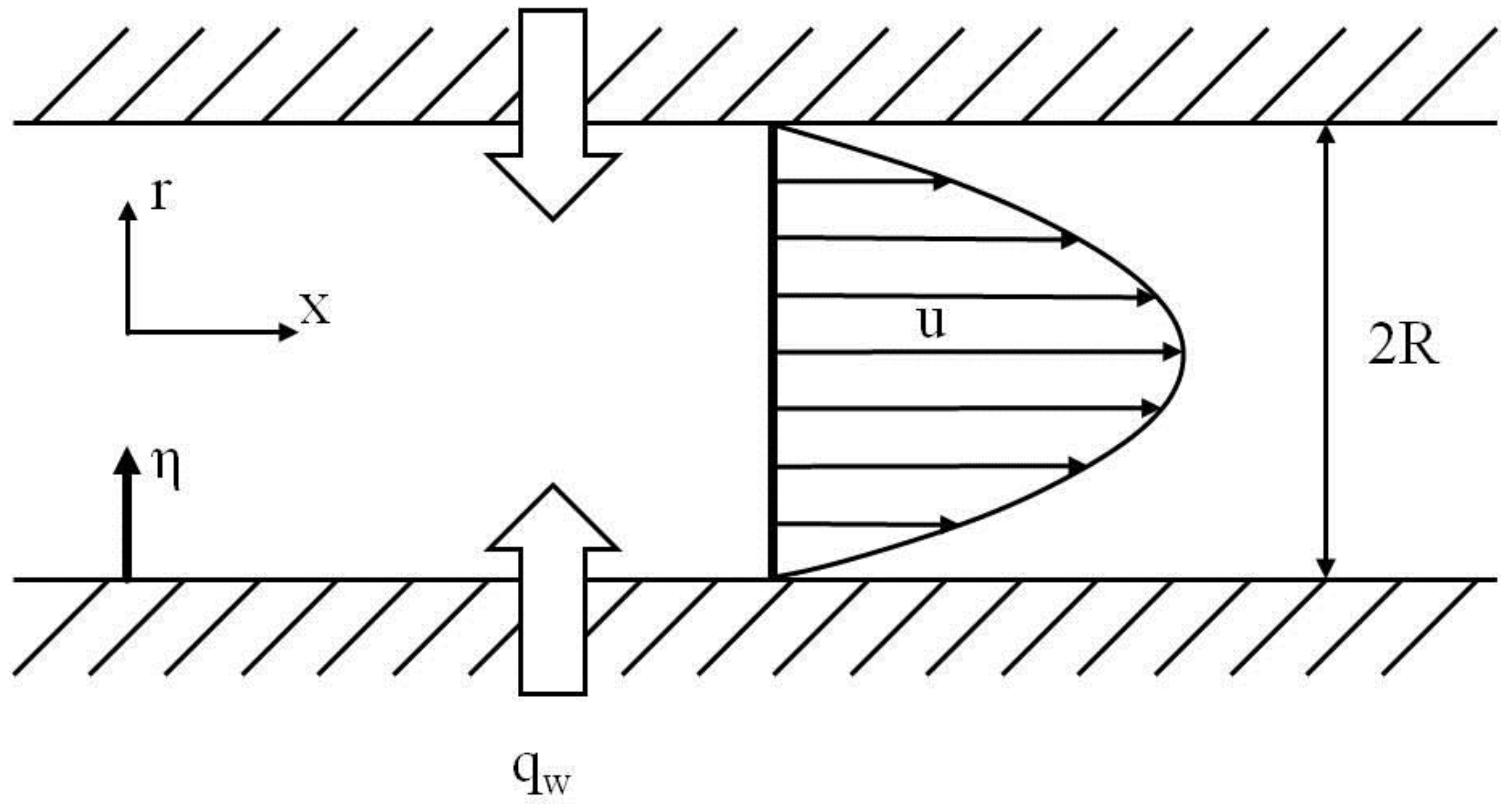
Before treating the cases of nanofluid saturated metal foam, we shall consider the fundamental case of clear nanofluid convective flow (i.e., without a metal foam), namely, hydrodynamically and thermally fully developed flow in a tube subject to constant heat flux. The problem may be descried mathematically by writing the governing equations in the cylindrical coordinates (x, r) shown in Figure 1 as

$$\frac{1}{r}\frac{d}{dr}\left(r\mu \frac{du}{dr}\right)-\frac{dp}{dx}=0$$

(7)

$$\rho cu\frac{\partial T}{\partial x}=\frac{1}{r}\frac{\partial }{\partial r}\left(rk\frac{\partial T}{\partial r}\right)$$

(8)

$$\frac{1}{r}\frac{d}{dr}\left(D_B\frac{d\varphi }{dr}+\frac{D_T}{T}\frac{dT}{dr}\right)=0$$

(9)

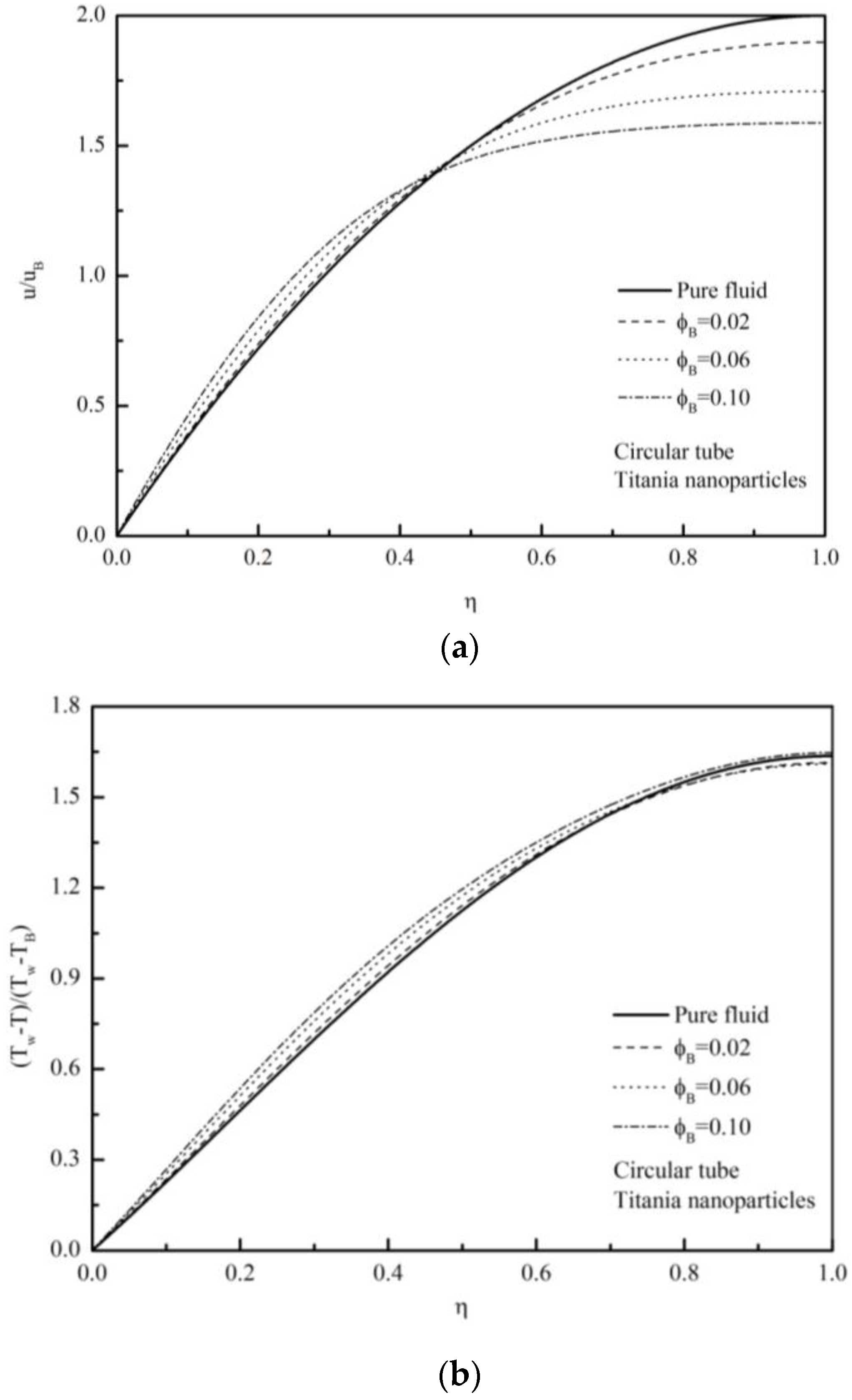
Yang et al. [23] transformed the preceding equations into the set of ordinary differential equations. This set of ordinary differential equations were integrated by using a versatile software SOLODE based on the Runge–Kutta–Gill method [21]. The effects of the bulk mean particle volume fraction ${\varphi }_B$ on the velocity profile $u/u_B$ are shown in Figure 2a for the case of titania–water nanofluids in a tube with $N_{BT}\equiv {D_B}_w{T}_w{\varphi }_w{k}_w/{D_T}_w{q}_{w}R$ = 0.2 and $\gamma \equiv q_{w}R/k_w{T}_w$ = 0. Likewise, the temperature profiles are presented in Figure 2b in terms of $\left(T_w-T\right)/\left(T_w-T_B\right)$. 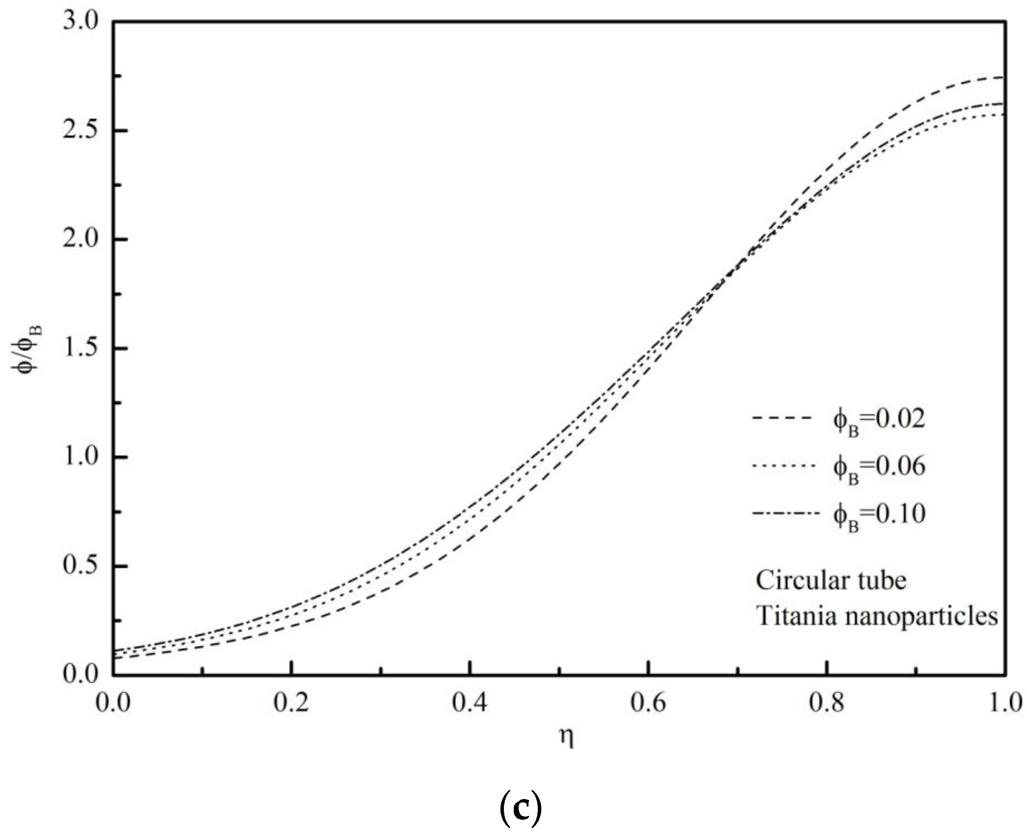Furthermore, the distributions of the particle volume fraction $\varphi /{\varphi }_B$ are shown in Figure 2c. The figure indicates low volume fraction of particles near the wall and high volume fraction of particles in the core. This uneven distribution of the volume fraction of particles is caused by the thermopheresis, which drives the particles from the high temperature region near the wall to the low temperature region in the core. The unevenness grows further as the thermopheretic diffusion dominates over the Brownian diffusion. Due to low and high volume fractions of nanoparticles, the viscosity near the wall surface, as given by Equation (5c), is much smaller than that in the core. This results in the increase in the velocity near the wall and the decrease in the velocity in the core, as can be confirmed in Figure 2a. This tendency is amplified as adding more particles. Figure 2b consistently shows that the increase in the dimensionless velocity near the wall leads to a steeper dimensionless temperature gradient as compared with the one with pure fluids (${\varphi }_B=0$). The effects of $\gamma$ on these profiles are found be almost negligible, as varying $\gamma$ from 0 to 0.1. Therefore, all calculations have been carried out with $\gamma$ = 0.

The Nusselt number based on the diameter $D_h=2R$ and the nanofluid bulk thermal conductivity $k_B=k\left({\varphi }_B\right)$ is given by

$$N{u}_B\equiv \frac{h{D}_h}{k_B}=\left(\frac{h{D}_h}{k_w}\right)\left(\frac{k_w}{k_B}\right)$$

(10)

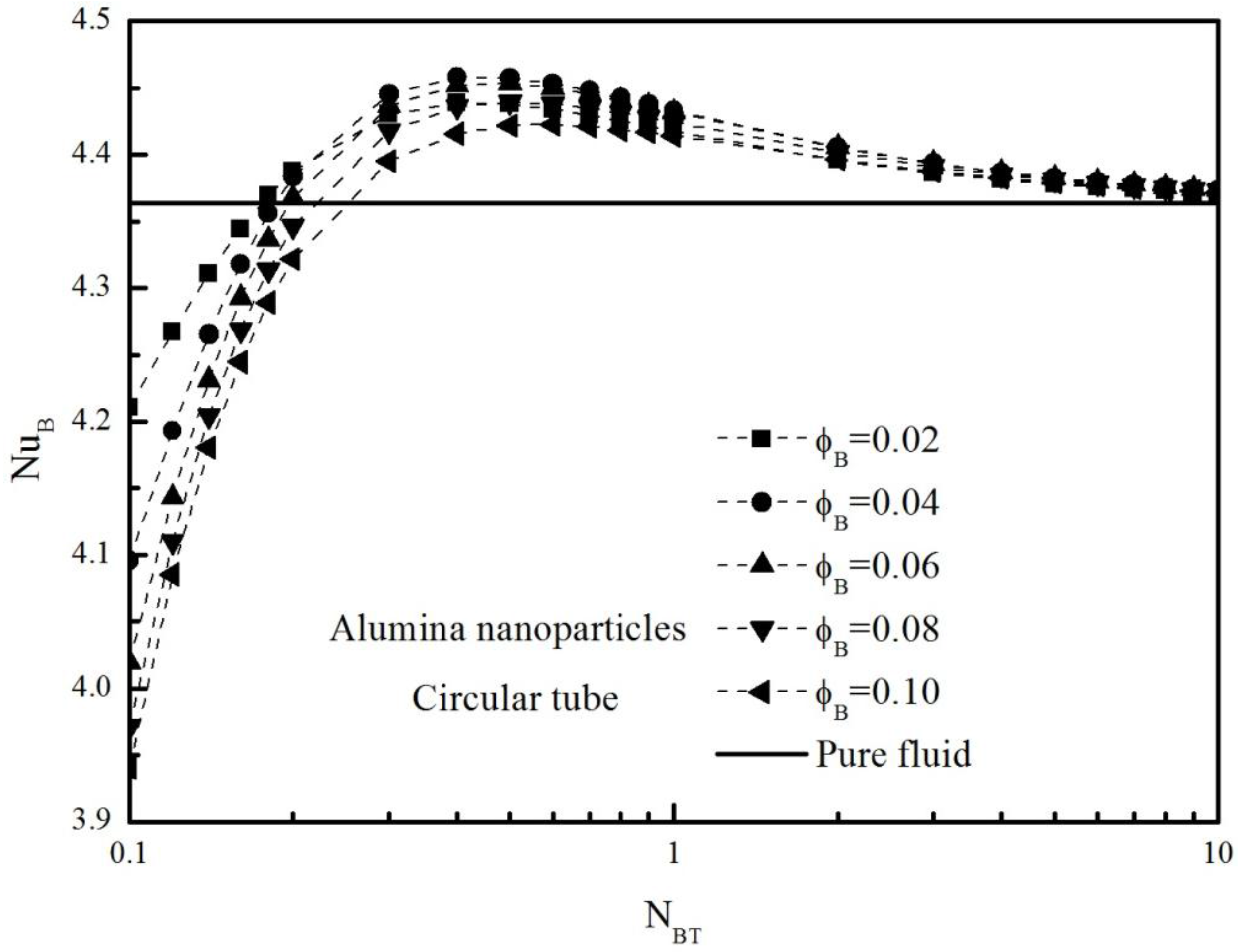
The Nusselt number $N{u}_B$ is expressed in terms of the product of the Nusselt number based on the thermal conductivity at the wall $h{D}_h/k_w$ and the thermal conductivity ratio $k_w/k_B$. This thermal conductivity ratio $k_w/k_B$ is always less than 1. Hence, the anomalous heat transfer enhancement, in which the heat transfer coefficient exceeds the level expected from the increase in the effective thermal properties of nanofluids, is possible only when the Nusselt number $h{D}_h/k_w$ is high enough to make its product (i.e., $N{u}_B$) more than that of pure fluid, namely, 4.36.

$N{u}_B$ for the case of alumina nanoparticles is shown in Figure 3, which the anomalous heat transfer enhancement can be seen clearly. Such heat transfer anomaly is absent for the case of channel flow. This difference observed in the heat transfer characteristic may be attributed to the geometrical (radial) effects, namely, that events taking place near the peripheral walls, such as velocity and temperature changes, reflect on bulk quantities more in a tube than in a channel. The maximum value of $N{u}_B$ is achieved at $N_{BT}\cong 0.5$ as shown in Figure 3. 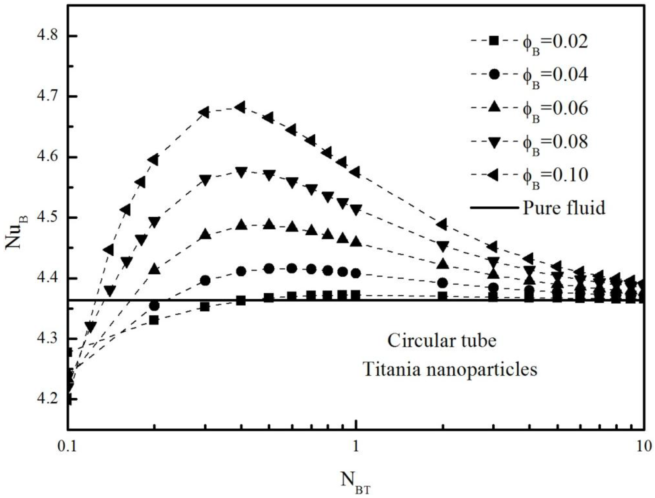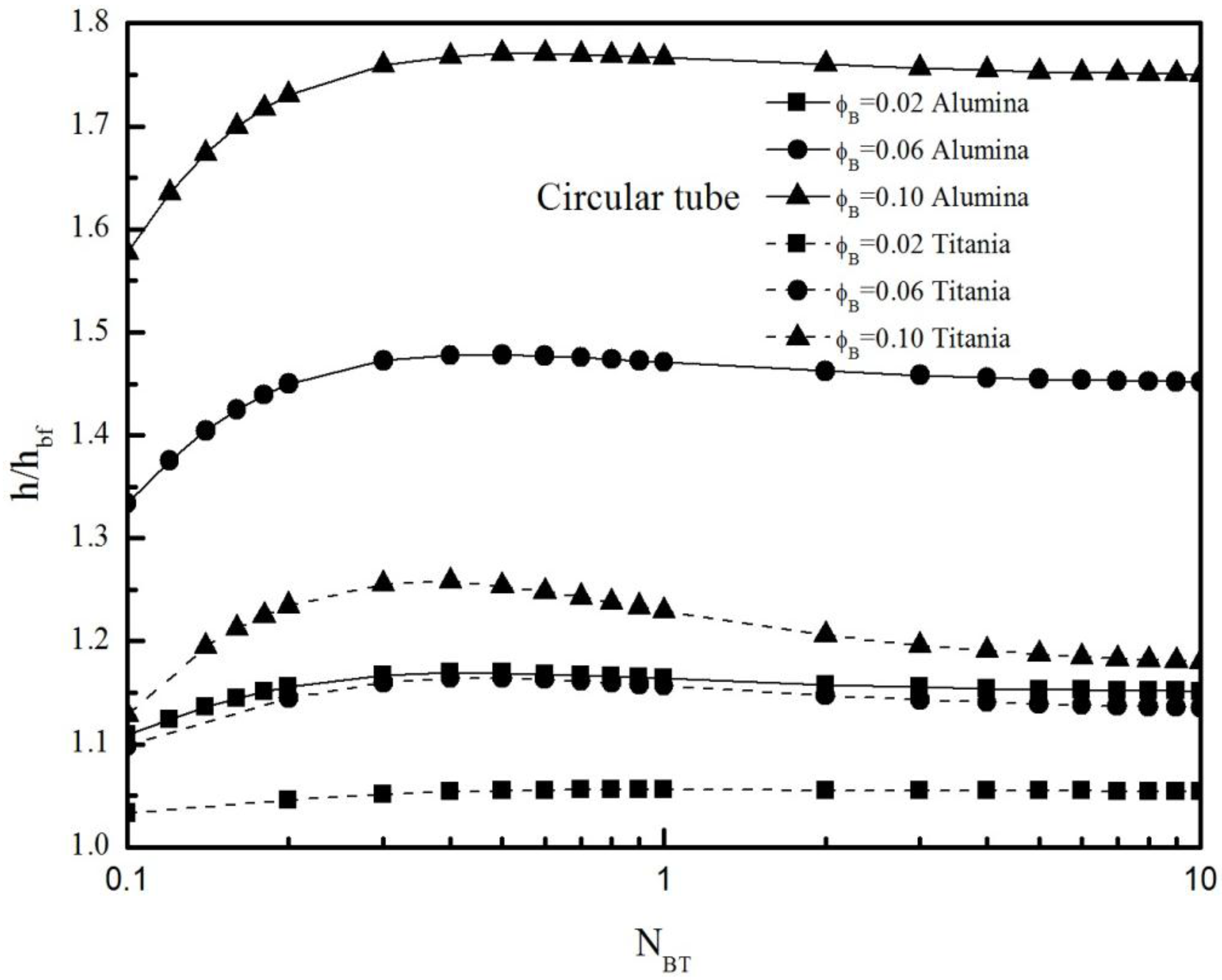Figure 4 clearly shows that the degree of the anomalous heat transfer enhancement in titania–water nanofluids is higher than in alumina–water nanofluids. However, as in Figure 5, the heat transfer coefficient of the alumina–water nanofluids is much higher than that of the titania–water nanofluids. This is simply due to the difference in $k_B$.

The analysis based on the Buongiorno model equations for convective heat transfer in clear nanofluid flows clearly indicates possible anomalous convective heat transfer enhancement. To be precise, the anomalous heat transfer enhancement has been captured theoretically for various cases of clear nanofluid flows, namely, the cases of titania–water nanofluids in a channel, alumina–water nanofluids in a tube and also titania–water nanofluids in a tube. Comparatively low volume fraction of particles near the wall is responsible for the anomalous heat transfer, because it yields a relatively low viscosity field there, hence, leading to high velocity and steep temperature gradient, near the wall. The maximum Nusselt number based on the bulk mean nanofluid thermal conductivity is observed around at $N_{BT}\cong 0.5$. This finding may be utilized for designing nanoparticles in view of heat transfer enhancement. Moreover, the heat transfer coefficient for the case of alumina–water nanofluids in a tube is seen almost twice higher than that of water in a tube. This substantiates the great potential of nanofluids as a high-energy carrier.

4. Volume Averaging theory

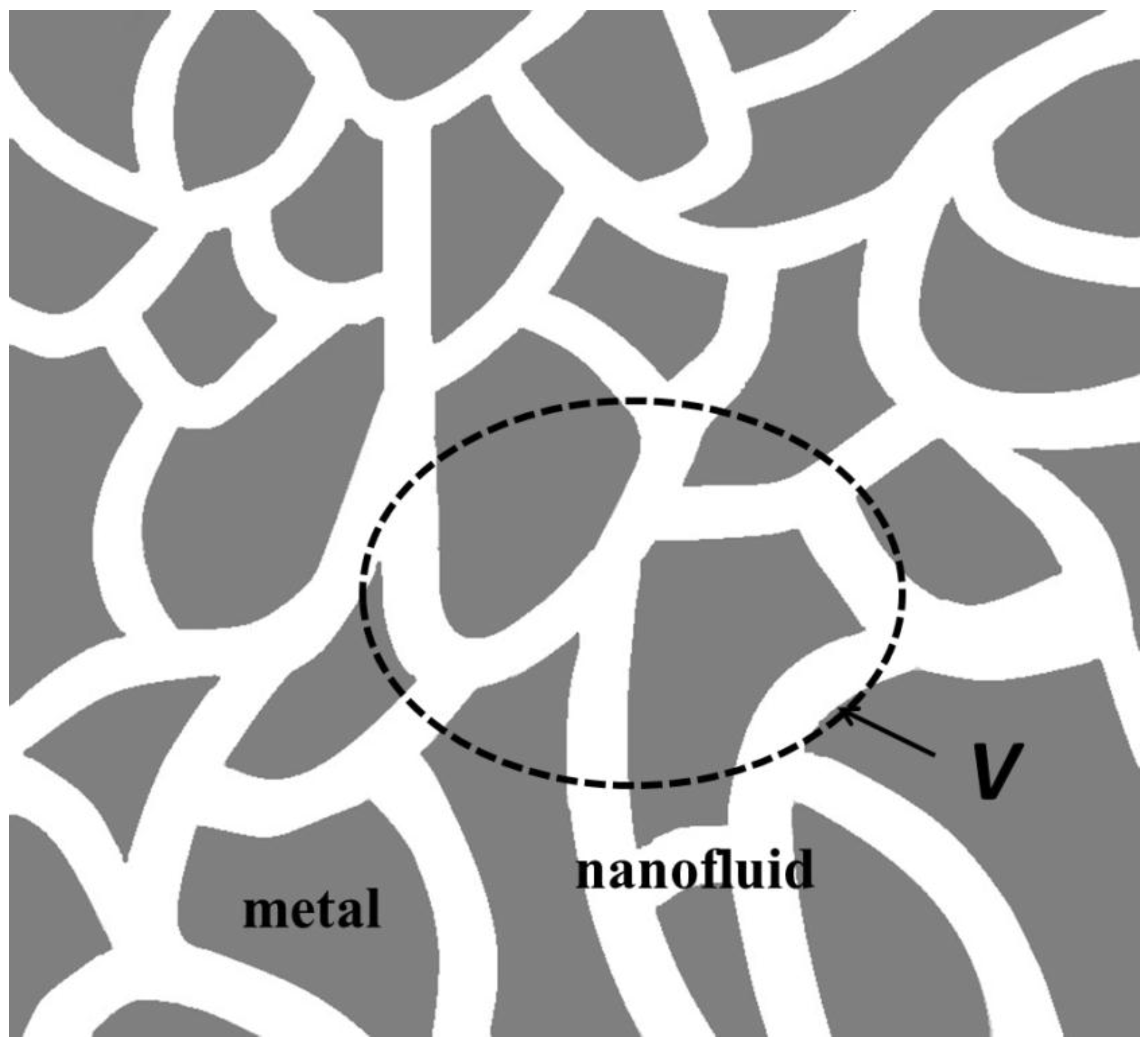
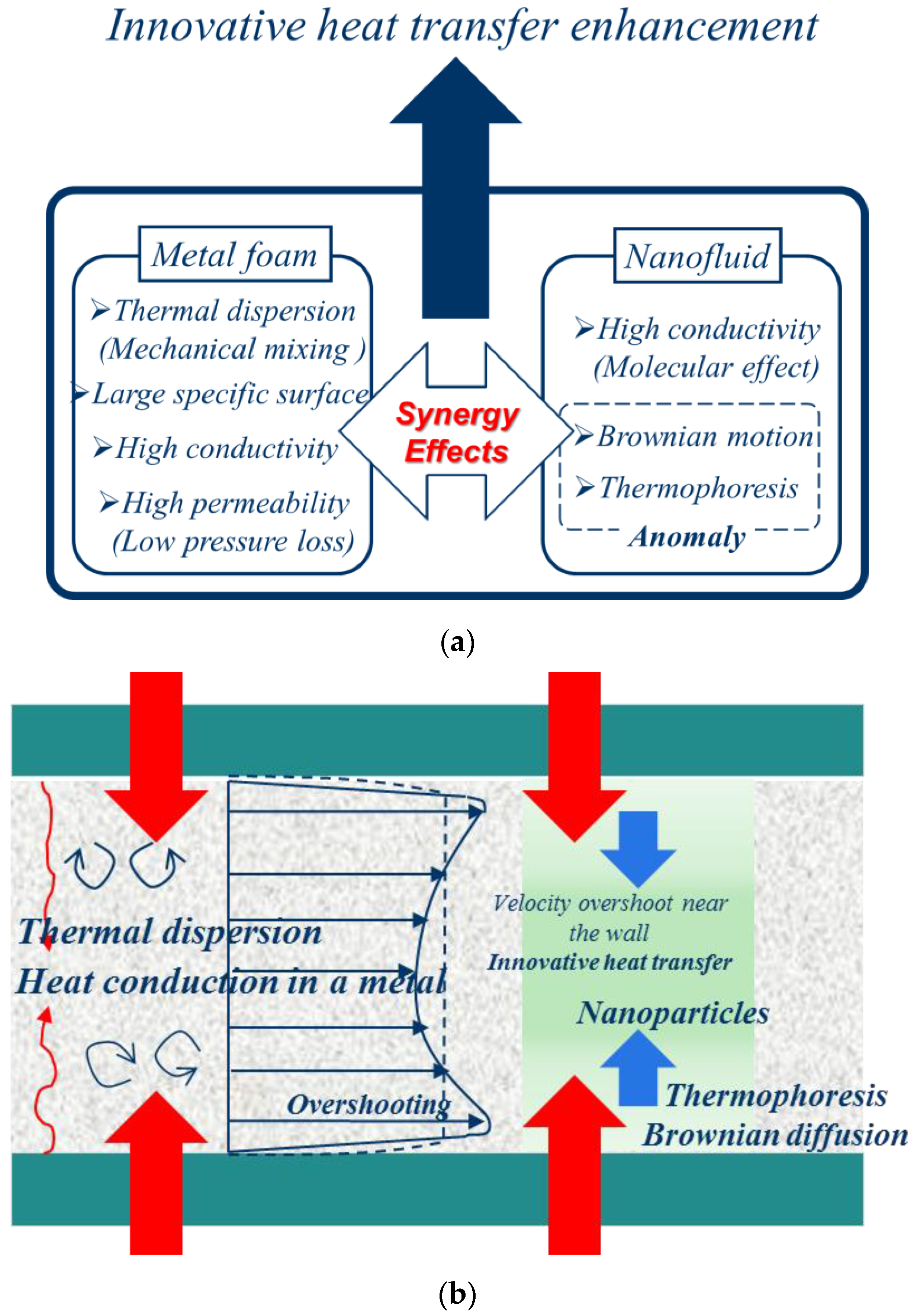
Having confirmed high heat transfer enhancement associated with nanofluids, we shall combine such nanofluids with metal foam, so as to form a passage filled with a nanofluid saturated metal foam. As illustrated in Figure 6a, we expect heat transfer enhancement associated with nanofluids, namely, the anomalous heat transfer resulting from both Brownian diffusion and thermophoretic diffusion, while high effective thermal conductivity and thermal dispersion (i.e., mechanical mixing) can also be expected from an embedded metal foam. These features, when combined together, may bring us the synergy effects on convective heat transfer. Figure 6b clearly indicates that the anomalous heat transfer enhancement in nanofluids, when taking place in a passage filled with a nanofluid saturated metal foam, further leads us to an innovative heat transfer enhancement. The velocity overshooting is expected in the near wall layer, which is partially responsible for the innovative heat transfer enhancement. This interesting feature will be numerically predicted later.

In order to investigate such an innovative heat transfer enhancement, we shall introduce a volume averaging procedure and seek a complete set of the macroscopic governing equations for convection within a nanofluid saturated metal foam.

Consider a local averaging volume $V$ in nanofluid saturated metal foam, as shown in Figure 7. Its length scale $V^{1/3}$ is much smaller than the macroscopic characteristic length, but, at the same time, much greater than the microscopic characteristic length (see, e.g., [18,19,20,21]). This condition allows us to define the volume average of a certain variable $\phi$ as

$$\langle \phi \rangle =\frac{1}{V}{\displaystyle {\int }_{V_f}\phi }dV$$

(11a)

Another average, namely, the intrinsic average, is given by

$${\langle \phi \rangle }^f=\frac{1}{V_f}{\displaystyle {\int }_{V_f}\phi }dV$$

(11b)

where $V_f$ is a volume space which nanofluid occupies. Obviously, two averages are related as $\langle \phi \rangle =\epsilon {\langle \phi \rangle }^f$, where $\epsilon =V_f/V$ is the porosity, namely, local volume fraction of the nanofluid phase. Let us decompose a variable into its intrinsic average and spatial deviation from it:

$$\phi ={\langle \phi \rangle }^f+\tilde{\phi }$$

(12)

All dependent variables in the microscopic governing equations for the nanofluid and metal phases are decomposed in this manner. The following spatial average relationships are used:

$${\langle {\phi }_1{\phi }_2\rangle }^f={\langle {\phi }_1\rangle }^f{\langle {\phi }_2\rangle }^f+{\langle {\tilde{\phi }}_1{\tilde{\phi }}_2\rangle }^f$$

(13)

$$\langle \frac{\partial \phi }{\partial x_i}\rangle =\frac{\partial \langle \phi \rangle }{\partial x_i}+\frac{1}{V}{\displaystyle {\int }_{A_{\mathrm{int}}}\phi n_i}dA$$

(14a)

$$\text{or }{\langle \frac{\partial \phi }{\partial x_i}\rangle }^f=\frac{1}{\epsilon }\frac{\partial \epsilon {\langle \phi \rangle }^f}{\partial x_i}+\frac{1}{V_f}{\displaystyle {\int }_{A_{\mathrm{int}}}\phi n_i}dA$$

(14b)

and

$$\langle \frac{\partial \phi }{\partial t}\rangle =\frac{\partial \langle \phi \rangle }{\partial t}$$

(15)

A_int represents the interfaces between fluid and solid matrix within a local averaging volume. Note N_i is the unit vector pointing outward from nanofluid side to solid side. All dependent variables for nanofluid and metal phases are decomposed according to Equation (12). Upon exploiting the foregoing spatial average relationships, the microscopic Equations (1) to (4) are integrated over a local averaging volume. The set of macroscopic governing equations thus obtained for nanofluid and metal phases in a nanofluid saturated metal foam with uniform porosity ε may be given as follows:

$$\frac{\partial \rho {\langle u_j\rangle }^f}{\partial x_j}+\frac{1}{V_f}{\displaystyle {\int }_{A_{\mathrm{int}}}\rho u_j}{n}_{j}dA=0$$

(16)

$$\begin{array}{l}\frac{\partial \rho {\langle u_i\rangle }^f}{\partial t}+\frac{\partial \rho {\langle u_j\rangle }^f{\langle u_i\rangle }^f}{\partial x_j}\\ =-\frac{\partial {\langle p\rangle }^f}{\partial x_i}+\frac{\partial }{\partial x_j}\left(\mu \left(\frac{\partial {\langle u_i\rangle }^f}{\partial x_j}+\frac{\partial {\langle u_j\rangle }^f}{\partial x_i}\right)+\frac{\mu }{V_f}{\displaystyle {\int }_{A_{\mathrm{int}}}\left(u_i{n}_j+u_j{n}_i\right)dA}-\rho {\langle {\tilde{u}}_i{\tilde{u}}_j\rangle }^f\right)+\frac{1}{V_f}{\displaystyle {\int }_{A_{\mathrm{int}}}\left(\mu \left(\frac{\partial u_i}{\partial x_j}+\frac{\partial u_j}{\partial x_i}\right)-p{\delta }_{ij}\right)}{n}_{j}dA-\frac{1}{V_f}{\displaystyle {\int }_{A_{\mathrm{int}}}\rho u_j{u}_i}{n}_{j}dA\end{array}$$

(17)

$$\epsilon c\left(\frac{\partial \rho {\langle T\rangle }^f}{\partial t}+\frac{\partial \rho {\langle u_j\rangle }^f{\langle T\rangle }^f}{\partial x_j}\right)=\frac{\partial }{\partial x_j}\left(\epsilon k\frac{\partial {\langle T\rangle }^f}{\partial x_j}+\frac{k}{V}{\displaystyle {\int }_{A_{\mathrm{int}}}T}{n}_{j}dA-\epsilon \rho c{\langle \tilde{T}{\tilde{u}}_j\rangle }^f\right)+\frac{1}{V}{\displaystyle {\int }_{A_{\mathrm{int}}}k\frac{\partial T}{\partial x_j}}{n}_{j}dA-\frac{c}{V}{\displaystyle {\int }_{A_{\mathrm{int}}}\rho T{u}_j}{n}_{j}dA$$

(18)

$$\left(1-\epsilon \right)c_s\frac{\partial {\langle T\rangle }^s}{\partial t}=\frac{\partial }{\partial x_j}\left(\left(1-\epsilon \right)k_s\frac{\partial {\langle T\rangle }^s}{\partial x_j}-\frac{k_s}{V}{\displaystyle {\int }_{A_{\mathrm{int}}}T}{n}_{j}dA\right)-\frac{1}{V}{\displaystyle {\int }_{A_{\mathrm{int}}}{k}_s\frac{\partial T}{\partial x_j}}{n}_{j}dA$$

(19)

$$\begin{array}{l}\frac{\partial {\langle \varphi \rangle }^f}{\partial t}+\frac{\partial {\langle u_j\rangle }^f{\langle \varphi \rangle }^f}{\partial x_j}\\ =\frac{\partial }{\partial x_j}\left(D_B\frac{\partial {\langle \varphi \rangle }^f}{\partial x_j}+\frac{D_T}{{\langle T\rangle }^f}\frac{\partial {\langle T\rangle }^f}{\partial x_j}+\frac{D_B}{V_f}{\displaystyle {\int }_{A_{\mathrm{int}}}\varphi }{n}_{j}dA+\frac{D_T}{V_f{\langle T\rangle }^f}{\displaystyle {\int }_{A_{\mathrm{int}}}T}{n}_{j}dA-{\langle \tilde{\varphi }{\tilde{u}}_j\rangle }^f\right)\\ +\frac{1}{V_f}{\displaystyle {\int }_{A_{\mathrm{int}}}\left(D_B\frac{\partial \varphi }{\partial x_j}+\frac{D_T}{{\langle T\rangle }^f}\frac{\partial T}{\partial x_j}\right)}{n}_{j}dA-\frac{1}{V_f}{\displaystyle {\int }_{A_{\mathrm{int}}}{u}_j\varphi }{n}_{j}dA\end{array}$$

(20)

Equation (19) is obtained integrating the conduction equation in a metal phase. In the foregoing equations, many interfacial terms vanish due to no-slip and no-particle flux conditions on the nanofluid–metal interface, namely,

$$u_j=\overrightarrow{0}\text{ and}$$

(21a)

$$\left(D_B\frac{\partial \varphi }{\partial x_j}+\frac{D_T}{T}\frac{\partial T}{\partial x_j}\right)n_j=0$$

(21b)

As these surface integral terms vanish, the equations reduce to

$$\frac{\partial \rho {\langle u_j\rangle }^f}{\partial x_j}=0$$

(22)

$$\frac{\partial \rho {\langle u_i\rangle }^f}{\partial t}+\frac{\partial \rho {\langle u_j\rangle }^f{\langle u_i\rangle }^f}{\partial x_j}=-\frac{\partial {\langle p\rangle }^f}{\partial x_i}+\frac{\partial }{\partial x_j}\left(\mu \left(\frac{\partial {\langle u_i\rangle }^f}{\partial x_j}+\frac{\partial {\langle u_j\rangle }^f}{\partial x_i}\right)-\rho {\langle {\tilde{u}}_i{\tilde{u}}_j\rangle }^f\right)+\frac{1}{V_f}{\displaystyle {\int }_{A_{b_{\mathrm{int}}}}\left(\mu \left(\frac{\partial u_i}{\partial x_j}+\frac{\partial u_j}{\partial x_i}\right)-p{\delta }_{ij}\right)}{n}_{j}dA$$

(23)

$$\epsilon c\left(\frac{\partial \rho {\langle T\rangle }^f}{\partial t}+\frac{\partial \rho {\langle u_j\rangle }^f{\langle T\rangle }^f}{\partial x_j}\right)=\frac{\partial }{\partial x_j}\left(\epsilon k\frac{\partial {\langle T\rangle }^f}{\partial x_j}+\frac{k}{V}{\displaystyle {\int }_{A_{\mathrm{int}}}T{n}_j}dA-\epsilon \rho c{\langle \tilde{T}{\tilde{u}}_j\rangle }^f\right)+\frac{1}{V}{\displaystyle {\int }_{A_{\mathrm{int}}}k\frac{\partial T}{\partial x_j}{n}_j}dA$$

(24)

$$\left(1-\epsilon \right)c_s\frac{\partial \rho {\langle T\rangle }^s}{\partial t}=\frac{\partial }{\partial x_j}\left(\left(1-\epsilon \right)k_s\frac{\partial {\langle T\rangle }^s}{\partial x_j}-\frac{k_s}{V}{\displaystyle {\int }_{A_{\mathrm{int}}}T{n}_j}dA\right)-\frac{1}{V}{\displaystyle {\int }_{A_{\mathrm{int}}}k\frac{\partial T}{\partial x_j}{n}_j}dA$$

(25)

$$\epsilon \left(\frac{\partial {\langle \varphi \rangle }^f}{\partial t}+\frac{\partial {\langle u_j\rangle }^f{\langle \varphi \rangle }^f}{\partial x_j}\right)=\frac{\partial }{\partial x_j}\left(\epsilon D_B\frac{\partial {\langle \varphi \rangle }^f}{\partial x_j}+\frac{\epsilon D_T}{{\langle T\rangle }^f}\frac{\partial {\langle T\rangle }^f}{\partial x_j}+\frac{D_B}{V}{\displaystyle {\int }_{A_{\mathrm{int}}}\varphi }{n}_{j}dA+\frac{D_T}{V{\langle T\rangle }^f}{\displaystyle {\int }_{A_{\mathrm{int}}}T}{n}_{j}dA-\epsilon {\langle \tilde{\varphi }{\tilde{u}}_j\rangle }^f\right)$$

(26)

In the foregoing equations, the correlations associated with deviations, $-\rho {\langle {\tilde{u}}_i{\tilde{u}}_j\rangle }^f$, $\epsilon \rho c{\langle \tilde{T}{\tilde{u}}_j\rangle }^f$ and $-\epsilon {\langle \tilde{\varphi }{\tilde{u}}_j\rangle }^f$, correspond with mechanical dispersion terms, whereas the surface integral terms, $\frac{k}{V}{\displaystyle {\int }_{A_{\mathrm{int}}}T{n}_j}dA$, $\frac{D_B}{V}{\displaystyle {\int }_{A_{\mathrm{int}}}\varphi }{n}_{j}dA$ and $\frac{D_T}{V{\langle T\rangle }^f}{\displaystyle {\int }_{A_{\mathrm{int}}}T}{n}_{j}dA$, correspond with the tortuosity terms.

5. Mathematical Modeling

As usual, Forchheimer-extended Darcy law is introduced to describe the internal flow resistance:

$$\frac{1}{V_f}{\displaystyle {\int }_{A_{\mathrm{int}}}\left(\mu \left(\frac{\partial u_i}{\partial x_j}+\frac{\partial u_j}{\partial x_i}\right)-p{\delta }_{ij}\right)}{n}_{j}dA\frac{\partial }{\partial x}\rho {\langle {\tilde{u}}_i{\tilde{u}}_j\rangle }^f=-\frac{\epsilon \mu }{K}{\langle u_j\rangle }^f-\rho {\epsilon }^{2}b\sqrt{{\langle u_k\rangle }^f{\langle u_k\rangle }^f}{\langle u_j\rangle }^f$$

(27)

while tortuosity in nanoparticle volume fraction transport is neglected since

$$\frac{D_B}{V_f}{\displaystyle {\int }_{A_{\mathrm{int}}}\varphi }{n}_{j}dA\cong \frac{D_B}{V_f}\varphi {\displaystyle {\int }_{A_{\mathrm{int}}}{n}_j}dA=\overrightarrow{0}$$

(28)

Tortuosity terms in two energy equations may be modeled introducing the Yang–Nakayama effective porosity $\epsilon *$ ([12,14]) as

$$\epsilon k\frac{\partial {\langle T\rangle }^f}{\partial x_j}+\frac{k}{V}{\displaystyle {\int }_{A_{\mathrm{int}}}T}{n}_{j}dA=\epsilon *k\frac{\partial {\langle T\rangle }^f}{\partial x_j}$$

(29a)

$$\left(1-\epsilon \right)k_s\frac{\partial {\langle T\rangle }^s}{\partial x_j}-\frac{k_s}{V}{\displaystyle {\int }_{A_{\mathrm{int}}}T}{n}_{j}dA=\left(1-\epsilon *\right)k_s\frac{\partial {\langle T\rangle }^s}{\partial x_j}$$

(29b)

where the effective porosity may easily be evaluated from

$${\epsilon }^{*}=\frac{k_s-k_{stag}}{k_s-k_f}$$

(30)

where $k_{stag}$ is the stagnant thermal conductivity of saturated porous medium, which can readily be measured using a standard method. However, for the cases of high conductivity porous media such as metal foams, satisfying the condition, $k_s/k>>3/(1-\epsilon )$, there is no need to measure the stagnant thermal conductivity of saturated porous medium, since the effective porosity may well be approximated by

$${\epsilon }^{*}=\frac{2+\epsilon }{3}$$

(31)

according to Yang and Nakayama (2010). For example, in the case of aluminum foam and water combination, we typically have $k_s/k\cong 330$ and $\epsilon =0.90$. Thus, $k_s/k>>3/(1-\epsilon )$ is satisfied such that ${\epsilon }^{*}=\left(2+0.9\right)/3=0.97$. Furthermore, Newton’s cooling law may be adopted for the interstitial heat transfer between nanofluid phase and metal foam as

$$\frac{1}{V}{\displaystyle {\int }_{A_{\mathrm{int}}}k\frac{\partial T}{\partial x_j}{n}_j}dA=h_v\left({\langle T\rangle }^s-{\langle T\rangle }^f\right)$$

(32)

where h_v is the volumetric interstitial heat transfer coefficient. Upon implementing the foregoing mathematical models, the equations reduce to

$$\frac{\partial \rho \langle u_j\rangle }{\partial x_j}=0$$

(33)

$$\frac{1}{\epsilon }\frac{\partial \rho \langle u_i\rangle }{\partial t}+\frac{1}{{\epsilon }^2}\frac{\partial \rho \langle u_j\rangle \langle u_i\rangle }{\partial x_j}=-\frac{\partial {\langle p\rangle }^f}{\partial x_i}+\frac{\partial }{\partial x_j}\left(\frac{\mu }{\epsilon }\frac{\partial \langle u_i\rangle }{\partial x_j}\right)-\frac{\mu }{K}\langle u_i\rangle -\rho b\sqrt{\langle u_k\rangle \langle u_k\rangle }\langle u_i\rangle$$

(34)

$$\epsilon c\frac{\partial \rho {\langle T\rangle }^f}{\partial t}+c\frac{\partial \rho \langle u_j\rangle {\langle T\rangle }^f}{\partial x_j}=\frac{\partial }{\partial x_j}\left({\epsilon }^{*}{k}_f\frac{\partial {\langle T\rangle }^f}{\partial x_j}-\epsilon \rho c{\langle \tilde{T}{\tilde{u}}_j\rangle }^f\right)-h_v\left({\langle T\rangle }^f-{\langle T\rangle }^s\right)$$

(35)

$$\left(1-\epsilon \right){\rho }_s{c}_s\frac{\partial {\langle T\rangle }^s}{\partial t}=\frac{\partial }{\partial x_j}\left(1-{\epsilon }^{*}\right)k_s\frac{\partial {\langle T\rangle }^s}{\partial x_j}-h_v\left({\langle T\rangle }^s-{\langle T\rangle }^f\right)=0$$

(36)

$$\epsilon \frac{\partial {\langle \varphi \rangle }^f}{\partial t}+\frac{\partial \langle u_j\rangle {\langle \varphi \rangle }^f}{\partial x_j}=\frac{\partial }{\partial x_j}\left(\epsilon D_B\frac{\partial {\langle \varphi \rangle }^f}{\partial x_j}+\frac{{\epsilon }^{*}{D}_T}{{\langle T\rangle }^f}\frac{\partial {\langle T\rangle }^f}{\partial x_j}-\epsilon {\langle \tilde{\varphi }{\tilde{u}}_j\rangle }^f\right)$$

(37)

Note that Equation (29a) is exploited to express the particle tortuosity term as

$$\frac{\epsilon D_T}{{\langle T\rangle }^f}\frac{\partial {\langle T\rangle }^f}{\partial x_j}+\frac{D_T}{V{\langle T\rangle }^f}{\displaystyle {\int }_{A_{\mathrm{int}}}T}{n}_{j}dA\cong \frac{\epsilon D_T}{{\langle T\rangle }^f}\frac{\partial {\langle T\rangle }^f}{\partial x_j}+\left(\epsilon *-\epsilon \right)\frac{D_T}{{\langle T\rangle }^f}\frac{\partial {\langle T\rangle }^f}{\partial x_j}=\frac{{\epsilon }^{*}{D}_T}{{\langle T\rangle }^f}\frac{\partial {\langle T\rangle }^f}{\partial x_j}$$

(38)

In the foregoing equations, Darcian velocity vector $\langle u_j\rangle =\epsilon {\langle u_j\rangle }^f$ is used in place of the intrinsic velocity vector ${\langle u_j\rangle }^f$.

6. Thermal Dispersion

Our next task in mathematical modelling is to mathematically model mechanical dispersion terms, namely, $-\epsilon \rho c{\langle \tilde{T}{\tilde{u}}_j\rangle }^f$ and $-\epsilon {\langle \tilde{\varphi }{\tilde{u}}_j\rangle }^f$, in terms of determinable variables. Measurement of mechanical dispersion, however, is quite formidable. Only a limited number of correlations for metal foams are available only for the case of transverse thermal dispersion. Empirical information is not available for longitudinal thermal dispersion in metal foams. As for the nanoparticle mechanical dispersion, neither theoretical nor empirical information exits so far.

Yang and Nakayama [14] claimed that volumetric interstitial heat transfer coefficient is comparatively easy to measure, using a standard method such as the single blow method [30]. Thus, they conducted an analytical consideration in a pore scale, and derived a theoretical relation to estimate thermal dispersion from the volumetric interstitial heat transfer coefficient, as illustrated below.

Along the macroscopic flow direction x, the nanofluid phase energy Equation (35) at steady state may be written as

$$c\rho \langle u\rangle \frac{\partial {\langle T\rangle }^f}{\partial x}\cong -h_v\left({\langle T\rangle }^f-{\langle T\rangle }^s\right)$$

(39)

where we have dropped diffusion term, since convection term on the left hand side predominates over axial diffusion term. A magnitude analysis [14] tells us that the diffusive term in Equation (35) is small and may well be neglected for the first approximation. This is usually true when an external scale of the flow system is much larger than a pore scale.

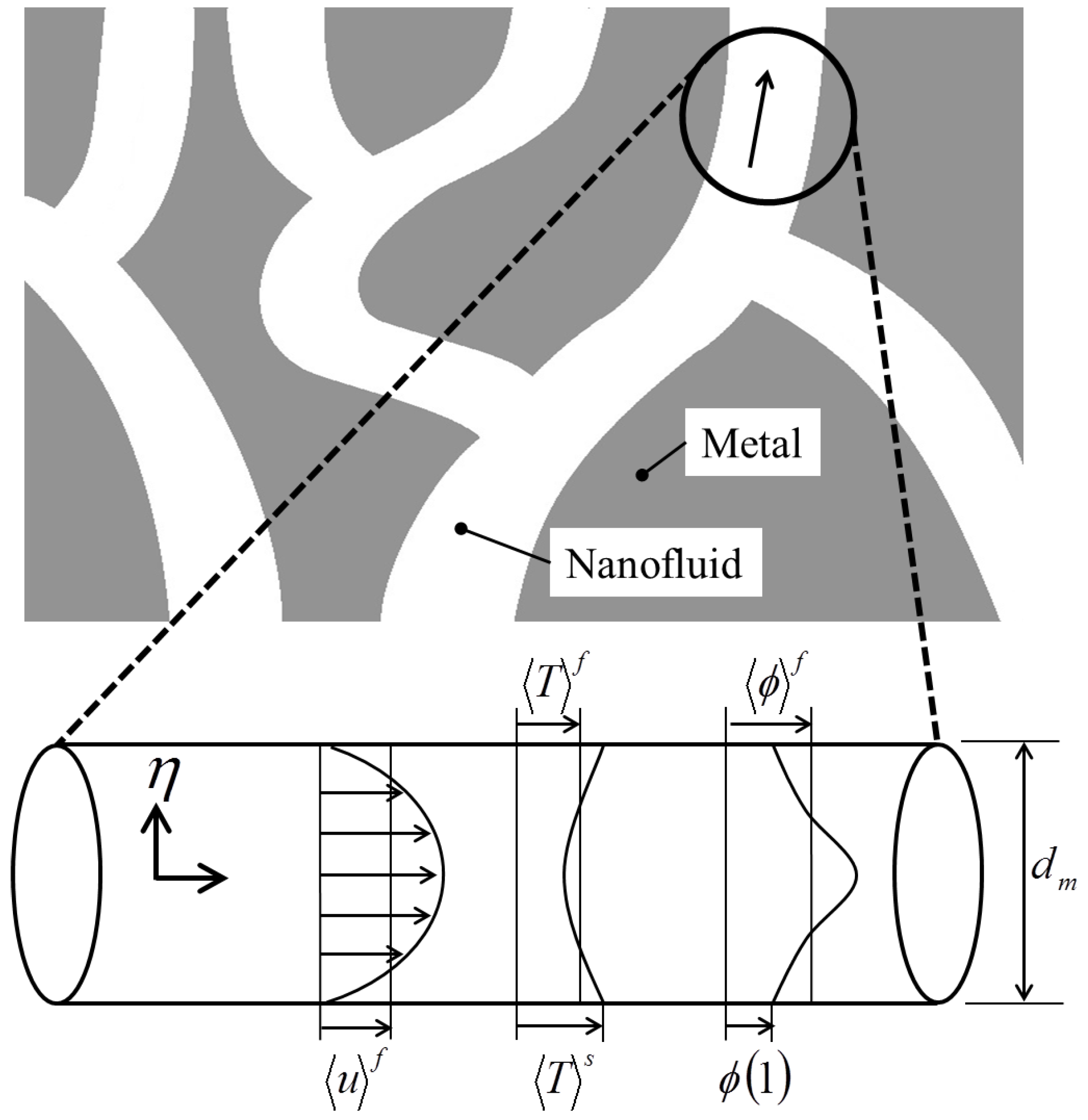
Let us consider a pore scale passage as illustrated in Figure 8. Longitudinal thermal dispersion term may be evaluated using microscopic velocity and temperature profiles prevailing in this pore scale passage as follows:

$$-\epsilon \rho c{\langle \tilde{T}\tilde{u}\rangle }^f=-\rho c\langle u\rangle \left({\langle T\rangle }^f-{\langle T\rangle }^s\right){\langle \left(f-1\right)\left(g-1\right)\rangle }^f=\frac{{\left(\rho c\langle u\rangle \right)}^2}{h_v}{\langle \left(f-1\right)\left(g-1\right)\rangle }^f\frac{\partial {\langle T\rangle }^f}{\partial x}$$

(40)

where the volume averaged temperature difference between two phases has been replaced by the volume averaged temperature gradient, exploiting the preceding macroscopic Equation (39). Hence,

$$-\epsilon \rho c{\langle \tilde{T}\tilde{u}\rangle }^f=\epsilon k_{di{s}_{xx}}\frac{\partial {\langle T\rangle }^f}{\partial x}$$

(41)

where

$$\epsilon k_{di{s}_{xx}}=\frac{{\left(\rho c\langle u\rangle \right)}^2}{h_v}{\langle \left(f-1\right)\left(g-1\right)\rangle }^f$$

(42)

which is consistent with what is known as gradient diffusion hypothesis [31]. For the volumetric interstitial heat transfer coefficient $h_v$ in Equation (42), the following empirical correlation proposed by Calmidi and Mahajan [3] may be used:

$$N{u}_v=\frac{h_v{d_m}^2}{k_f}=8.72{\left(1-\epsilon \right)}^{1/4}{\left(\frac{1-e^{-\left(1-\epsilon \right)/0.04}}{\epsilon }\right)}^{1/2}{\left(\frac{\langle u\rangle d_m}{\nu }\right)}^{1/2}P{r}^{0.37}$$

(43)

where $d_m$ is the pore diameter. The correlation is based on the one developed by Zhukauskas [32] for cylinders in laminar cross flow. Note that the functions $f\left(\eta \right)$ and $g\left(\eta \right)$ describe the velocity and temperature profiles, respectively, in a pore passage of diameter $d_m$ as illustrated in Figure 8.

$$u={\langle u\rangle }^{f}f\left(\eta \right)$$

(44a)

and

$$T-{\langle T\rangle }^s=\left({\langle T\rangle }^f-{\langle T\rangle }^s\right)g\left(\eta \right)$$

(44b)

where the dimensionless radial coordinate $\eta$ normal to the pore wall is defined as

$$\eta =2r/d_m$$

(45)

Any reasonable functions may be used for $f\left(\eta \right)$ and $g\left(\eta \right)$ in Equation (42) to estimate $k_{di{s}_{xx}}$ such as laminar fully developed velocity and temperature profiles in a tube with its diameter $d_m$:

$$f\left(\eta \right)=2\left(1-{\eta }^2\right)$$

(46a)

and

$$g\left(\eta \right)=\frac{3}{4}\left(3-4{\eta }^2+{\eta }^4\right)$$

(46b)

Note that ${\langle f\left(\eta \right)\rangle }^f={\displaystyle {\int }_0^{1}2\eta f\left(\eta \right)d\eta =1}$ and ${\langle g\left(\eta \right)\rangle }^f={\displaystyle {\int }_0^{1}2\eta g\left(\eta \right)d\eta =1}$. Substituting the foregoing profiles into Equation (42) along with Equation. (43), we readily obtain Longitudinal (laminar):

$$\frac{\epsilon k_{di{s}_{xx}}}{k}=\frac{{\left(\rho c\langle u\rangle \right)}^2}{h_{v}k}{\langle \left(f-1\right)\left(g-1\right)\rangle }^f=\frac{3}{8N{u}_v}{\left(\frac{\rho c\langle u\rangle d_m}{k}\right)}^2=\frac{3}{8}\frac{{\left(\frac{\rho c\langle u\rangle d_m}{k}\right)}^{3/2}P{r}^{0.13}}{8.72{\left(1-\epsilon \right)}^{1/4}{\left(\frac{1-e^{-\left(1-\epsilon \right)/0.04}}{\epsilon }\right)}^{1/2}}$$

(47)

A similar relationship can be derived for the transverse thermal dispersion. Let us consider the energy Equation (35) close enough to a heated wall surface for convection to be negligible, but at the same time, sufficiently away from the wall surface, so that the transverse thermal dispersion dominates over the stagnant thermal diffusion:

$$\epsilon k_{di{s}_{yy}}\frac{d^2{\langle T\rangle }^f}{d{r}^2}\cong h_v\left({\langle T\rangle }^f-{\langle T\rangle }^s\right)$$

(48)

which may be integrated to yield

$$\frac{d{\langle T\rangle }^f}{dr}=-\sqrt{\frac{h_v}{\epsilon k_{di{s}_{yy}}}}\left({\langle T\rangle }^f-{\langle T\rangle }^s\right)$$

(49)

such that

$$-\epsilon \rho c_p{\langle \tilde{v}\tilde{T}\rangle }^f\equiv \epsilon k_{di{s}_{yy}}\frac{d{\langle T\rangle }^f}{dr}=-\rho c_p\langle u\rangle \left({\langle T\rangle }^f-{\langle T\rangle }^s\right){\langle F\left(g-1\right)\rangle }^f=\rho c_p\langle u\rangle \sqrt{\frac{{\epsilon k_{dis}}_{yy}}{h_v}}{\langle F\left(g-1\right)\rangle }^f\frac{d{\langle T\rangle }^f}{dr}$$

(50)

Hence,

$$\epsilon k_{di{s}_{yy}}=\frac{{\left(\rho c\langle u\rangle \right)}^2}{h_v}{\left({\langle F\left(g-1\right)\rangle }^f\right)}^2$$

(51)

where

$$v=\tilde{v}={\langle u\rangle }^{f}F\left(\eta \right)$$

(52)

such that ${\langle F\left(\eta \right)\rangle }^f={\langle v\rangle }^f/{\langle u\rangle }^f=0$. Equation (51) obtained for the transverse thermal dispersion conductivity is the same as Equation (42) obtained for the longitudinal thermal dispersion conductivity, except the difference in the multiplicative constants, namely, ${\left({\langle F\left(g-1\right)\rangle }^f\right)}^2$ and ${\langle \left(f-1\right)\left(g-1\right)\rangle }^f$. It is understood that $\left|F\left(\eta \right)\right|$<<1. In fact, the experimental data on packed bed reported by Fried and Combarnous [33] suggest that ${\left({\langle F\left(g-1\right)\rangle }^f\right)}^2$ is much smaller than ${\langle \left(f-1\right)\left(g-1\right)\rangle }^f$. In this study, we assume ${\left({\langle F\left(g-1\right)\rangle }^f\right)}^2\cong {\langle \left(f-1\right)\left(g-1\right)\rangle }^f/{15}^2$, such that Transverse (laminar):

$$\begin{array}{l}\frac{\epsilon k_{di{s}_{yy}}}{k}=\frac{{\left(\rho c\langle u\rangle \right)}^2}{h_{v}k}{\left({\langle F\left(g-1\right)\rangle }^f\right)}^2\\ =\frac{3}{{15}^2\times 8}\frac{{\left(\frac{\rho c\langle u\rangle d_m}{k}\right)}^{3/2}P{r}^{0.13}}{8.72{\left(1-\epsilon \right)}^{1/4}{\left(\frac{1-e^{-\left(1-\epsilon \right)/0.04}}{\epsilon }\right)}^{1/2}}=0.00019\frac{{\left(\frac{\rho c\langle u\rangle d_m}{k}\right)}^{3/2}P{r}^{0.13}}{{\left(1-\epsilon \right)}^{1/4}{\left(\frac{1-e^{-\left(1-\epsilon \right)/0.04}}{\epsilon }\right)}^{1/2}}\end{array}$$

(53)

In order to estimate the longitudinal thermal dispersion for the case of fully turbulent flow, a similar procedure is used along with the wall laws as

$$u=u_{\tau }\left(\frac{1}{\kappa }\ln n^{+}+B\right)$$

(54a)

and

$$T-{\langle T\rangle }^s=-\frac{q_w{\sigma }_T}{u_{\tau }{\rho }_f{c}_{pf}}\left(\frac{1}{\kappa }\ln n^{+}+A\right)$$

(54b)

where $u_{\tau }$ and $q_w$ are friction velocity and wall heat flux, respectively, and $n^{+}=u_{\tau }n/\nu$ is a dimensionless distance measured from the wall surface ($n=\left(d_m-2r\right)/2$). Moreover, $\kappa$ is the von-Karman constant while both B and A are empirical constants. It is easy to find

$$\tilde{u}=\frac{u_{\tau }}{\kappa }\left(\ln \varsigma +\frac{3}{2}\right)$$

(55a)

and

$$\tilde{T}=-\frac{q_w{\sigma }_T}{u_{\tau }\rho c\kappa }\left(\ln \varsigma +\frac{3}{2}\right)$$

(55b)

where

$$\varsigma =1-\eta$$

(56)

Hence,

$$\begin{array}{l}-\epsilon \rho c{\langle \tilde{T}\tilde{u}\rangle }^f=\epsilon k_{di{s}_{xx}}\frac{\partial {\langle T\rangle }^f}{\partial x}=\frac{q_w{\sigma }_T}{{\kappa }^2}{\langle {\left(\ln \varsigma +\frac{3}{2}\right)}^2\rangle }^f=\frac{{\sigma }_T}{{\kappa }^2}{\langle {\left(\ln \varsigma +\frac{3}{2}\right)}^2\rangle }^f\frac{\rho c\langle u\rangle }{a_f}\frac{d{\langle T\rangle }^f}{dx}\\ =\frac{{\sigma }_T}{4\epsilon {\kappa }^2}\left(\frac{5}{4}\right)\rho c\langle u\rangle d_m\frac{d{\langle T\rangle }^f}{dx}\end{array}$$

(57)

where we used Equation (39) to eliminate the wall heat flux $q_w=-\left(h_v/a_f\right)\left({\langle T\rangle }^f-{\langle T\rangle }^s\right)$ with specific surface $a_f=4\epsilon /d_m$ in favor of the temperature gradient. Setting $\kappa$ and ${\sigma }_T$ to 0.41 and 0.9, respectively, according to Launder and Spalding [34], we obtain for the turbulent regime.

Longitudinal (turbulent regime):

$$\frac{\epsilon k_{di{s}_{xx}}}{k}=\frac{{\sigma }_T}{4\epsilon {\kappa }^2}\left(\frac{5}{4}\right)\frac{\rho c\langle u\rangle d_m}{k}=\frac{1.67}{\epsilon }\left(\frac{\rho c\langle u\rangle d_m}{k}\right)$$

(58)

Law of the wall was introduced by Taylor [35] to explain high Peclet number dependence observed in dispersion of matter in a pipe flow. The same linear relationship between the thermal dispersion conductivity and Peclet number (as observed experimentally) may easily be deducted using an interstitial heat transfer coefficient correlation, which increases linearly with Peclet number. This linear relationship between the thermal dispersion coefficient and Peclet number was explained theoretically by Nakayama et al. [36] for high Peclet number flow through a consolidated porous medium.

As for the transverse dispersion, we again assume $k_{di{s}_{yy}}\equiv {15}^2{k_{dis}}_{xx}$, such that Transverse (turbulent regime):

$$\frac{\epsilon k_{di{s}_{yy}}}{k}=\frac{{\sigma }_T}{4\epsilon {\kappa }^2}\left(\frac{5}{4}\right)\frac{\rho c\langle u\rangle d_m}{k}=\frac{1.67}{{15}^2\epsilon }\left(\frac{\rho c\langle u\rangle d_m}{k}\right)=\frac{0.00742}{\epsilon }\left(\frac{\rho c\langle u\rangle d_m}{k}\right)$$

(59)

As for experimental data on metal foams, only those of transverse thermal dispersion are available. The data for transverse dispersion coefficient have been correlated by Calmidi and Mahajan [3] as follows:

Transverse (Calmidi–Mahajan):

$$\frac{\epsilon k_{di{s}_{yy}}}{k}=0.00162\frac{\left(\frac{\rho c\langle u\rangle d_m}{k}\right)}{{\left({\left(1-\epsilon \right)}^{0.224}{\left(\frac{1.18}{1-e^{-\left(1-\epsilon \right)/0.04}}\sqrt{\frac{1-\epsilon }{3\pi }}\right)}^{1.11}\right)}^{1/2}}$$

(60)

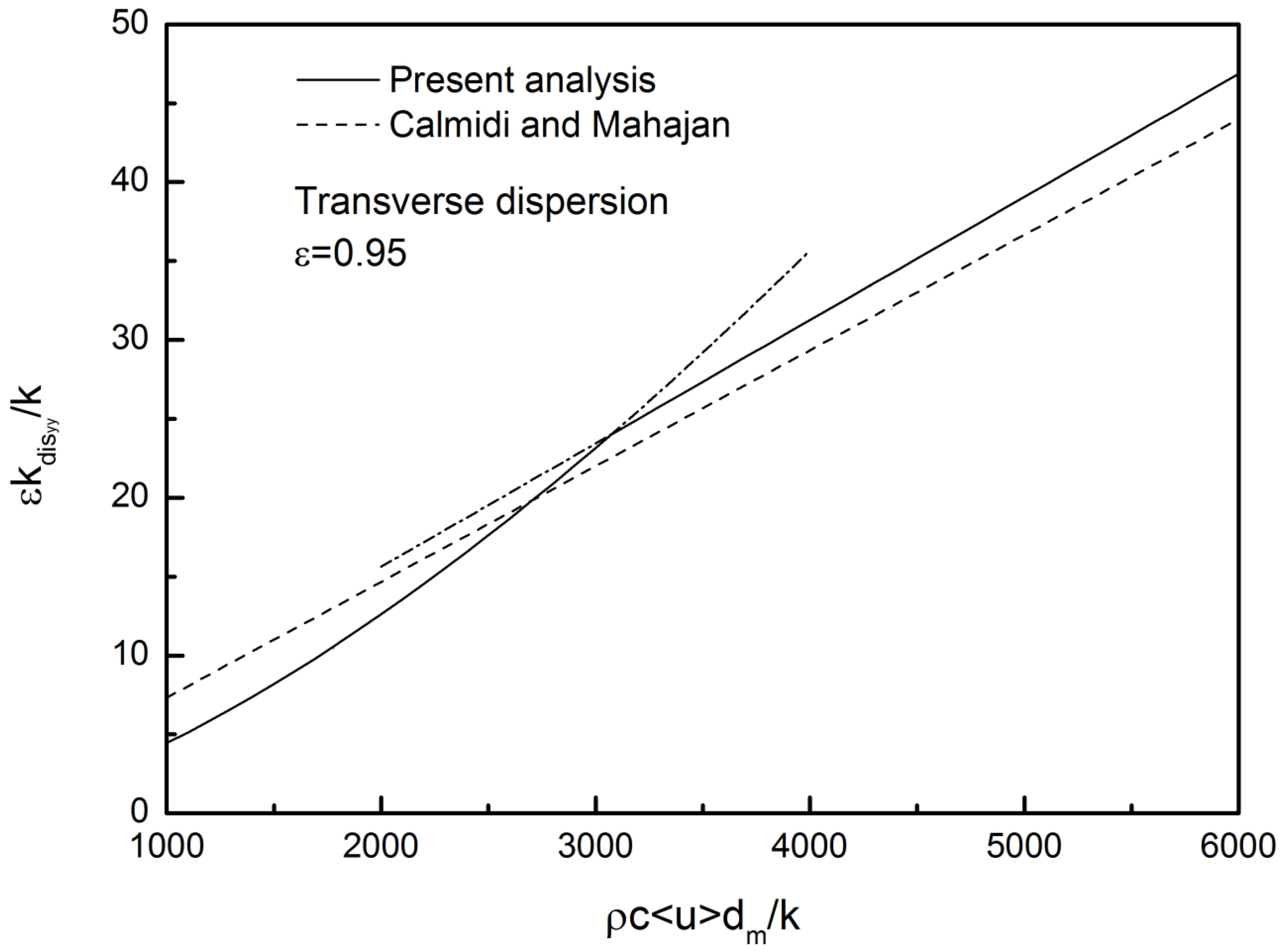
Thus, in Figure 9, Equation (53) for the laminar case and Equation (59) for the turbulent case are plotted together to form a solid curve for the case of $\epsilon$ = 0.95. In the figure, the foregoing empirical correlation Equation (60) is also plotted to examine the validity of the present expressions for the transverse dispersion coefficient. The figure shows fairly good agreement between the solid line based on the present analysis and the dashed empirical line reported by Calmidi and Mahajan. It is noted that Calmidi and Mahajan’s correlation is valid only when the Peclet number $\left(\rho c\langle u\rangle d_m/k\right)$ is sufficiently large. Taylor [37] analytically proved that the dispersion coefficient is in proportion to ${\left(\rho c\langle u\rangle d_m/k\right)}^2$, that is consistent with our Equation (47) for the case of small Peclet number, in which the interstitial heat transfer coefficient stays constant. It is also interesting to note that Gelhar and Axness [38] and Wang and Kitanidis [39] investigated macrodispersion in heterogeneous porous media such as aquifers and geologic formations. They reported Peclet number dependence similar to what is observed in Figure 9. Moreover, Ohsawa [40] in his MS thesis carried out direct numerical simulations for nanofluid forced convection using a numerically generated periodic open-cell. The thermal dispersion numerically predicted by him closely follows the empirical correlation Equation (60) up to Peclet number up to 10,000, or even more. Therefore, the empirical correlation Equation (60) may well be valid in the range as indicated in Figure 9.

7. Nanoparticle Mechanical Dispersion

For the first time, we shall introduce a mathematical model for the nanoparticle mechanical dispersion. The nanoparticle conservation Equation (37) at steady state is written along the macroscopic flow direction x, as

$$\frac{\partial \langle u\rangle {\langle \varphi \rangle }^f}{\partial x}=\frac{\partial }{\partial x}\left(\epsilon D_B\frac{\partial {\langle \varphi \rangle }^f}{\partial x}+\frac{{\epsilon }^{*}{D}_T}{{\langle T\rangle }^f}\frac{\partial {\langle T\rangle }^f}{\partial x}-\epsilon {\langle \tilde{\varphi }\tilde{u}\rangle }^f\right)$$

(61)

As illustrated in Figure 8, we consider nanoparticle conservation along a pore scale conduit with its diameter $d_m$. Thus, nanoparticle mechanical dispersion flux $-\epsilon {\langle \tilde{\varphi }{\tilde{u}}_j\rangle }^f$ can be expressed as

$$-\epsilon {\langle \tilde{\varphi }\tilde{u}\rangle }^f=-\langle u\rangle {\langle \varphi \rangle }^f{\langle \left(f-1\right)\left(G-1\right)\rangle }^f$$

(62)

where

$$\varphi ={\langle \varphi \rangle }^{f}G\left(\eta \right)$$

(63)

Function $G\left(\eta \right)$ for the nanoparticle profile may be estimated by solving Equation (4) in a pore conduit:

$$D_B\frac{d\varphi }{dr}+\frac{D_T}{T}\frac{dT}{dr}=0$$

(64)

which can easily be solved with Equations (6a) and (6b) being substituted:

$$\frac{\varphi \left(\eta \right)}{\varphi \left(1\right)}=\exp \left({\frac{D_T}{\varphi D_B}|}_{\eta =1}\left(\frac{{\langle T\rangle }^s}{T\left(\eta \right)}-1\right)\right)\cong 1+\frac{{\langle T\rangle }^s-{\langle T\rangle }^f}{{\langle T\rangle }^s}{\frac{D_T}{\varphi D_B}|}_{\eta =1}g\left(\eta \right)$$

(65)

since $\left({\langle T\rangle }^s-{\langle T\rangle }^f\right)/{\langle T\rangle }^s<<1$. Thus,

$$G\left(\eta \right)=\frac{\varphi \left(1\right)}{{\langle \varphi \rangle }^f}\left(1+\frac{{\langle T\rangle }^s-{\langle T\rangle }^f}{{\langle T\rangle }^s}{\frac{D_T}{\varphi D_B}|}_{\eta =1}g\left(\eta \right)\right)=\frac{1+\frac{{\langle T\rangle }^s-{\langle T\rangle }^f}{{\langle T\rangle }^s}{\frac{D_T}{\varphi D_B}|}_{\eta =1}g\left(\eta \right)}{1+\frac{{\langle T\rangle }^s-{\langle T\rangle }^f}{{\langle T\rangle }^s}{\frac{D_T}{\varphi D_B}|}_{\eta =1}}$$

(66)

Using Equation (46a,b) for velocity and temperature profiles, respectively, we readily obtain

$${\langle \left(f-1\right)\left(G-1\right)\rangle }^f=\frac{3}{8\left(1+n_{BT}\right)}\cong \frac{3}{8n_{BT}}$$

(67)

Thus

$$-\epsilon {\langle \tilde{\varphi }\tilde{u}\rangle }^f=-\frac{3}{8n_{BT}}\langle u\rangle {\langle \varphi \rangle }^f$$

(68)

where

$$n_{BT}\left({\langle T\rangle }^f,{\langle T\rangle }^s\right)=\frac{{\langle T\rangle }^s}{{\langle T\rangle }^s-{\langle T\rangle }^f}{\frac{\varphi D_B}{D_T}|}_{\eta =1}$$

(69)

is a dimensionless function of local volume averaged temperatures, describing the ratio of Brownian and thermophoretic diffusions within a pore conduit, as introduced by Yang et al. [23]. Note that absolute value of $n_{BT}$ in most cases is very large, and that, under local thermal equilibrium condition, namely, ${\langle T\rangle }^s={\langle T\rangle }^f$, grows infinitely. Equation (68) may be substituted into Equation (61) to yield

$$\frac{\partial \langle u\rangle {\langle \varphi \rangle }^f}{\partial x}\cong \frac{1}{1+\frac{3}{8n_{BT}}}\frac{\partial }{\partial x}\left(\epsilon D_B\frac{\partial {\langle \varphi \rangle }^f}{\partial x}+\frac{{\epsilon }^{*}{D}_T}{{\langle T\rangle }^f}\frac{\partial {\langle T\rangle }^f}{\partial x}\right)$$

(70)

Hence, nanoparticle mechanical dispersion works either to suppress or to enhance effective diffusion, as can be seen from the denominator $\left(1+3/8n_{BT}\right)$. It suppresses effective diffusion where the local temperature of metal foam phase is higher than that of nanofluid phase (i.e., $n_{BT}$ > 0). On the other hand, it enhances the diffusion where the local temperature of metal foam phase is lower than that of nanofluid phase (i.e., $n_{BT}$ < 0). However, this effect of nanoparticle mechanical dispersion on the effective diffusion is limited only to a moderate range of $n_{BT}$, where local thermal non-equilibrium is discernible. In the region where $n_{BT}$ is very large under nearly local thermal equilibrium, the nanoparticle mechanical dispersion flux $-\epsilon {\langle \tilde{\varphi }\tilde{u}\rangle }^f$, vanishes, and only stagnant particle diffusion remains. In this way, nanoparticle mechanical dispersion flux varies across the channel, depending on the degree of local thermal non-equilibrium there.

We shall again consider the nanoparticle conservation Equation (37) close enough to the wall surface for convection to be negligible:

$$\frac{\partial }{\partial y}\left(\epsilon D_B\frac{\partial {\langle \varphi \rangle }^f}{\partial y}+\frac{{\epsilon }^{*}{D}_T}{{\langle T\rangle }^f}\frac{\partial {\langle T\rangle }^f}{\partial y}-\epsilon {\langle \tilde{\varphi }\tilde{v}\rangle }^f\right)\cong \frac{\partial }{\partial y}\left(\epsilon D_B\frac{\partial {\langle \varphi \rangle }^f}{\partial y}+\frac{{\epsilon }^{*}{D}_T}{{\langle T\rangle }^f}\frac{\partial {\langle T\rangle }^f}{\partial y}\right)\cong 0$$

(71)

The nanoparticle mechanical dispersion flux $-\epsilon {\langle \tilde{\varphi }\tilde{v}\rangle }^f$ near the wall surface may be estimated as follows:

$$-\epsilon {\langle \tilde{\varphi }\tilde{v}\rangle }^f=-\epsilon {\langle \tilde{\varphi }\tilde{u}\rangle }^f\frac{{\langle F\left(G-1\right)\rangle }^f}{{\langle \left(f-1\right)\left(G-1\right)\rangle }^f}~\frac{\langle u\rangle {\langle \varphi \rangle }^f}{120n_{BT}}$$

(72)

Thus, the transverse nanoparticle mechanical dispersion is so small that it can totally be neglected, irrespective of the degree of local thermal non-equilibrium. Due to no-flux condition at the wall, Equation (71) naturally reduces to

$$\epsilon D_B\frac{\partial {\langle \varphi \rangle }^f}{\partial y}+\frac{{\epsilon }^{*}{D}_T}{{\langle T\rangle }^f}\frac{\partial {\langle T\rangle }^f}{\partial y}=0$$

(73)

Unfortunately, no experimental data are available for either transverse or longitudinal coefficients of nanoparticle mechanical dispersion.

8. Mathematical Model for Hydro-Dynamically and Thermally Fully Developed Flows

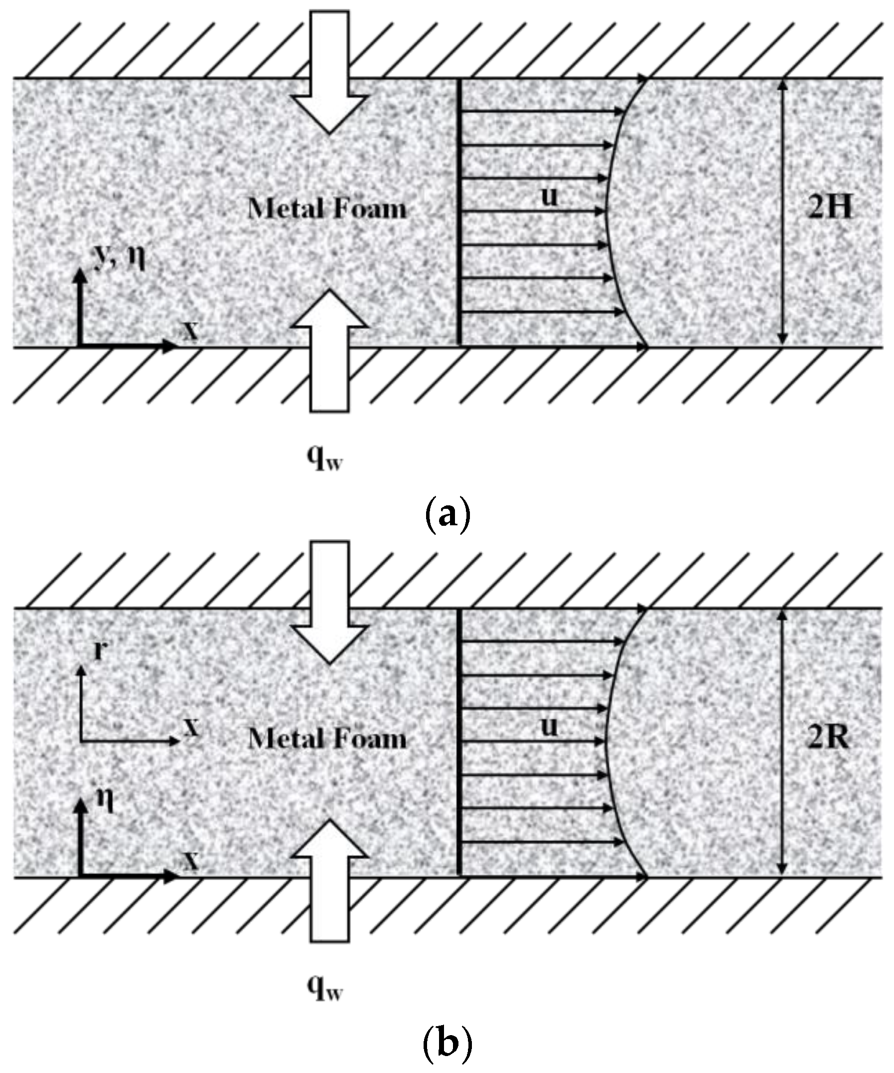
We shall refer to Figure 10, and consider hydrodynamically and thermally fully developed flows in both channel and tube subject to constant heat flux, filled with a nanofluid saturated metal foam. The walls are subject to axially constant heat flux and circumferentially constant wall temperature (i.e., constant heat flux everywhere).

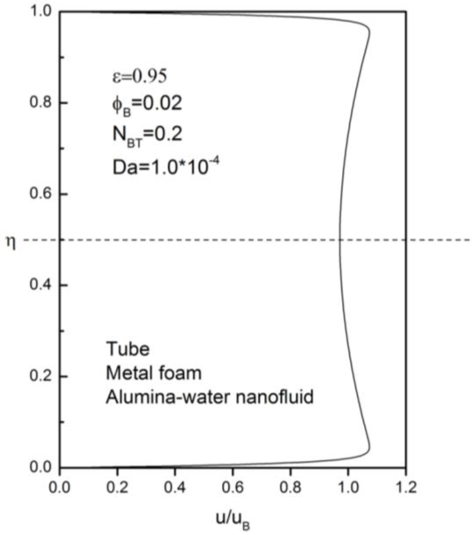
The macroscopic momentum Equation (34) can be numerically solved along with the macroscopic continuity Equation (33) for the case of fully developed flow in a tube. Such a volume averaged velocity profile is presented in Figure 11, in which the velocity is seen higher close to the wall, since the viscosity there is lower. This overshooting of the velocity works to carry heat effectively away from the heated wall.

In the following analytical treatment, however, the momentum Equation (34) is simplified using Forchheimer extended Darcy law, in which Brinkman term (i.e., macroscopic viscous diffusion term) is dropped, allowing the Darcian velocity slip on the wall. This Forchheimer extended Darcy law is valid for most of metal foams except for the case of extremely high permeability. Thus, for this case of the channel flow, the volume average Equations (33) to (37) reduce to:

$$-\frac{d{\langle p\rangle }^f}{dx}=\frac{{\mu }_f}{K}\langle u\rangle +\rho b{\langle u\rangle }^2$$

(74)

$$\rho c\langle u\rangle \frac{\partial {\langle T\rangle }^f}{\partial x}=\frac{\partial }{\partial y}\left({\epsilon }^{*}{k}_f+{\zeta }_k\rho c{d}_m\langle u\rangle \right)\frac{\partial {\langle T\rangle }^f}{\partial y}-h_v\left({\langle T\rangle }^f-{\langle T\rangle }^s\right)$$

(75)

$$\frac{\partial }{\partial y}\left(1-{\epsilon }^{*}\right)k_s\frac{\partial {\langle T\rangle }^s}{\partial y}-h_v\left({\langle T\rangle }^s-{\langle T\rangle }^f\right)=0$$

(76)

$$\frac{\partial }{\partial y}\left(\epsilon D_B\frac{\partial {\langle \varphi \rangle }^f}{\partial y}+\frac{{\epsilon }^{*}{D}_T}{{\langle T\rangle }^f}\frac{\partial {\langle T\rangle }^f}{\partial y}\right)=0$$

(77)

Following Equations (59), transverse thermal dispersion coefficient may be evaluated from

$${\zeta }_k=\frac{0.00742}{\epsilon }$$

(78)

Moreover, the interstitial volumetric coefficient $h_v$ is evaluated from Equation (43). Note that the continuity equation yields $\partial \langle u\rangle /\partial x=0$ and $\langle v\rangle =0$.

The origin of vertical coordinate y is set on the lower wall. The boundary conditions are given by

$$q_0=-\left({\epsilon }^{*}{k}_f+{\zeta }_k\rho c{d}_m\langle u\rangle \right){\frac{\partial {\langle T\rangle }^f}{\partial y}|}_{y=0}-\left(1-{\epsilon }^{*}\right)k_s{\frac{\partial {\langle T\rangle }^s}{\partial y}|}_{y=0}$$

(79)

$${\epsilon D_B\frac{\partial {\langle \varphi \rangle }^f}{\partial y}|}_{y=0}+\frac{{\epsilon }^{*}{D}_T}{{\langle T\rangle }^f}{\frac{\partial {\langle T\rangle }^f}{\partial y}|}_{y=0}=0$$

(80)

$${\frac{\partial {\langle \varphi \rangle }^f}{\partial y}|}_{y=H}=0$$

(81a)

$${\frac{\partial {\langle T\rangle }^f}{\partial y}|}_{y=H}={\frac{\partial {\langle T\rangle }^s}{\partial y}|}_{y=H}=0$$

(81b)

Kuwahara et al. [12] considered two extreme cases for possible wall temperature difference between solid and fluid phases, namely, locally uniform heat flux wall and locally thermal equilibrium wall, and concluded that the locally thermal equilibrium wall is much closer to the reality. Hence, we assume:

$${{\langle T\rangle }^s|}_{y=0}={{\langle T\rangle }^f|}_{y=0}\equiv T_0\left(x\right):\text{ wall temperature}$$

(82)

where $T_0\left(x\right)$ is the wall temperature. $T_0\left(x\right)$ increases linearly downstream under constant heat flux. Nanoparticle conservation Equation (77) indicates that diffusion mass flux of nanoparticles is constant across the channel. Since the wall is impermeable, the boundary condition Equation (80) holds such that effective Brownian diffusion flux and effective thermophoretic diffusion flux cancel out everywhere across the channel. Energy Equations (75) and (76) may be added together and integrated over the lower half channel from y = 0 to H with boundary conditions Equations (79) and (80) to give

$$\overline{\rho c\langle u\rangle }\frac{d{T}_B}{dx}=\frac{q_0}{H}$$

(83)

where the subscript 0 refers to the wall at $y=0$, and

$$\overline{\phi }\equiv \frac{1}{A}{\displaystyle {\int }_A\phi }dA=\frac{1}{H}{\displaystyle {\int }_0^H\phi }dy$$

(84)

denotes the average value over the cross-section such that

$$T_B\equiv \overline{\frac{\rho c\langle u\rangle \langle T\rangle }{\overline{\rho c\langle u\rangle }}}$$

(85a)

is the bulk mean temperature. Likewise, quantities with subscript B denote bulk quantities such as

$${\varphi }_B\equiv \overline{\langle u\rangle {\langle \varphi \rangle }^f}/\overline{\langle u\rangle }$$

(85b)

$$u_B\equiv \overline{\rho \langle u\rangle }/\rho \left({\varphi }_B\right)$$

(85c)

The foregoing considerations on both nanoparticle diffusion flux and axial temperature gradient will be implemented to obtain analytical expressions in a dimensionless form. The momentum Equation (74) may be arranged in a dimensionless form as

$$u*\left(y*\right)=\frac{\sqrt{1+4D{a}^{2}Hg\frac{\left(\rho /{\rho }_0\right)}{{\left(\mu /{\mu }_0\right)}^2}}-1}{2DaHg\frac{\left(\rho /{\rho }_0\right)}{\left(\mu /{\mu }_0\right)}}$$

(86)

Thus, for the case of Forchheimer extended Darcy flow (i.e., $Da<<1$), the velocity profile is described algebraically as the viscosity of nanofluid is provided as function of the nanoparticle volume fraction. The other governing equations are given in differential forms as follows:

$$\frac{\rho cu*}{\overline{\rho cu*}}=-\frac{d}{dy*}\left({\epsilon }^{*}\frac{k}{k_{stag0}}+{\zeta }_{k}Pe\frac{\rho c}{{\left(\rho c\right)}_0}u*\right)\frac{dT{*}^f}{dy*}+N{u}_v\left(T{*}^f-T{*}^s\right)$$

(87)

$$\left(1-\epsilon *\right)\frac{k_s}{k_{stag0}}\frac{d^{2}T{*}^s}{dy{*}^2}-N{u}_v\left(T{*}^s-T{*}^f\right)=0$$

(88)

$$\frac{d{\langle \varphi \rangle }^f}{dy*}=\frac{\epsilon *{\langle \varphi \rangle }^f}{\epsilon N_{BT}{\left(1-\gamma T{*}^f\right)}^2}\frac{dT{*}^f}{dy*}$$

(89)

Dimensionless coordinate, velocity and temperature are defined as

$$y*=y/H$$

(90)

$$u*=\langle u\rangle /\left(\frac{H^2}{{\mu }_0}\left(-\frac{d{\langle p\rangle }^f}{dx}\right)\right)$$

(91a)

$$T{*}^f=\frac{k_{stag0}\left(T_0-{\langle T\rangle }^f\right)}{q_{0}H}$$

(91b)

$$T{*}^s=\frac{k_{stag0}\left(T_0-{\langle T\rangle }^s\right)}{q_{0}H}$$

(91c)

$$N_{BT}\equiv \frac{D_{B0}{T}_0{\varphi }_0{k}_{stag0}}{D_{T0}{q}_{0}H}=\frac{D_{B0}{\varphi }_0}{D_{T0}\gamma }$$

(92a)

$$\gamma \equiv \frac{q_{0}H}{k_{stag0}{T}_0}$$

(92b)

Furthermore, Darcy, Lewis, Peclet, and Hagen numbers are defined as follows:

$$Da\equiv K/H^2$$

(93a)

$$Le\equiv k_{stag0}/{\left(\rho c\right)}_0{D}_{B0}$$

(93b)

$$Pe\equiv \frac{{\rho }_0{c}_0\sqrt{K}}{k_{stag0}}\frac{H^2}{{\mu }_0}\left(-\frac{d{\langle p\rangle }^f}{dx}\right)$$

(93c)

$$Hg\equiv \frac{{\rho }_{0}b{H}^4}{{{\mu }_0}^2}\left(-\frac{d{\langle p\rangle }^f}{dx}\right)$$

(93d)

where the properties with subscript 0 should be evaluated at the wall according to Equations (5a) to (6b), (30) and (31). For example, the stagnation thermal conductivity at wall where ${{\langle \varphi \rangle }^f|}_{y*=0}={\varphi }_0$ may be evaluated according to Equations (5d), (30) and (31) as

$$k_{stag0}=\epsilon *{k|}_{y*=0}+\left(1-\epsilon *\right)k_s=\frac{2+\epsilon }{3}\left(1+2.72{\varphi }_0+4.97{{\varphi }_0}^2\right)k_{bf}+\frac{1-\epsilon }{3}{k}_s$$

(94)

The dimensionless parameter $N_{BT}$ is related to the ratio of macroscopic Brownian and thermophoretic diffusivities. $N_{BT}$ can range over a wide range from 0.1 to 10 for typical cases of alumina and copper nanoparticles with $d_p$ ~10 nm and the bulk mean particle volume fraction ${\varphi }_B$ ~0.01. The ratio of wall and fluid temperature difference to absolute temperature, namely, $\gamma ~\left(T_0-{\langle T\rangle }_B^f\right)/T_0$, is usually much smaller than unity, as estimated by Buongiorno [17]. Similarity between “microscopic” ratio $n_{BT}$ (Equation (69)) and “macroscopic” ratio $N_{BT}$ (Equation (92a)) is worth noting, since the former describes the local ratio of microscopic Brownian and thermophoretic diffusivities in a pore scale, whereas the latter describes the ratio of macroscopic Brownian and thermophoretic diffusivities in a channel filled with a nanofluid saturated metal foam.

In reality, the bulk mean particle volume fraction ${\varphi }_B$ is given, while that at the wall ${\varphi }_0$ is unknown. However, for the sake of computational convenience, ${\varphi }_0$ is prescribed and ${\varphi }_B$ is calculated later to find out ${\varphi }_0$ as a function of ${\varphi }_B$.

The energy Equations (87) and (88) can be combined to form a third order Ordinary Differential Equation (O.D.E.) with respect to $T{*}^s$ as

$$\frac{d^{3}T{*}^s}{dy{*}^3}=N{u}_v\frac{\left(\frac{k_{stag}}{k_{stag0}}+{\zeta }_{k}Pe\frac{\rho c}{{\left(\rho c\right)}_0}u*\right)\frac{dT{*}^s}{dy*}-{\displaystyle {\int }_{\eta }^1\frac{\rho cu*}{\overline{\rho cu*}}}dy*}{\left({\epsilon }^{*}\frac{k_f}{k_{stag0}}+{\zeta }_{k}Pe\frac{\rho c}{{\left(\rho c\right)}_0}u*\right)\left(1-{\epsilon }^{*}\right)\frac{k_s}{k_{stag0}}}$$

(95)

where

$$T{*}^f=T{*}^s-\frac{\left(1-\epsilon *\right)}{N{u}_v}\frac{k_s}{k_{stag0}}\frac{d^{2}T{*}^s}{dy{*}^2}$$

(96)

and Equation (89) can easily be integrated with ${{\langle \varphi \rangle }^f|}_{y*=0}={\varphi }_0$ to obtain

$$\frac{{\langle \varphi \rangle }^f}{{\varphi }_0}=\exp \left(\frac{\epsilon *T{*}^f}{N_{BT}\epsilon \left(1-\gamma T{*}^f\right)}\right)$$

(97)

The foregoing third order O.D.E. Equation (95) may easily be solved by using a standard integration scheme such as Runge–Kutta–Gill method (e.g., [21]). Appropriate boundary conditions for the equation are given by

$${T{*}^s|}_{y*=0}={\frac{d^{2}T{*}^s}{dy{*}^2}|}_{y*=0}=0$$

(98a)

$$\text{and }{\frac{dT{*}^s}{dy*}|}_{y*=1}=0$$

(98b)

which are based on the original boundary conditions given by Equations (81b) and (82).

A similar procedure based on the cylindrical coordinate system as shown in Figure 10b readily yields the following set of transformed equations for the case of circular tube:

$$\frac{d^{3}T{*}^s}{dy{*}^3}-\frac{1}{1-y*}\frac{d^{2}T{*}^s}{dy{*}^2}-\frac{1}{{\left(1-y*\right)}^2}\frac{dT{*}^s}{dy*}=N{u}_v\frac{\left(\frac{k_{stag}}{k_{stag0}}+{\zeta }_{k}Pe\frac{{\rho }_f{c}_f}{{\rho }_{f0}{c}_{f0}}u*\right)\frac{dT{*}^s}{dy*}-\frac{2}{1-y*}{\displaystyle {\int }_{y*}^1\frac{{\rho }_f{c}_{f}u*}{\overline{\rho cu*}}}\left(1-y*\right)dy*}{\left({\epsilon }^{*}\frac{k_f}{k_{stag0}}+{\zeta }_{k}Pe\frac{{\rho }_f{c}_f}{{\rho }_{f0}{c}_{f0}}u*\right)\left(1-{\epsilon }^{*}\right)\frac{k_s}{k_{stag0}}}$$

(99)

where

$$T{*}^f=T{*}^s-\frac{\left(1-\epsilon *\right)}{N{u}_v}\frac{k_s}{k_{stag0}}\left(\frac{d^{2}T{*}^s}{dy{*}^2}-\frac{1}{1-y*}\frac{dT{*}^s}{dy*}\right)$$

(100)

The boundary conditions in the cylindrical coordinate are the same as those given by Equation (98a,b). Moreover, Equation (97) for the volume averaged nanoparticle volume fraction holds also for the case of cylindrical coordinate system. However, note that the average value $\overline{\phi }$ for the case of the tube is computed by

$$\overline{\phi }\equiv \frac{1}{A}{\displaystyle {\int }_A\phi }dA=\frac{1}{\pi R^2}{\displaystyle {\int }_0^{R}2\pi r\phi }dr=2{\displaystyle {\int }_0^1\left(1-y*\right)}\phi dy*$$

(101)

where $y*=\left(R-r\right)/R$. The corresponding dimensionless quantities $u*$ to $N{u}_v$ are defined just as presented in Equations (91a) to (93d) replacing the channel half height H by the tube radius R.

9. Results and Discussion

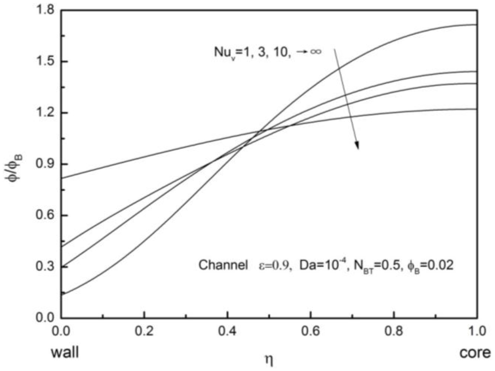
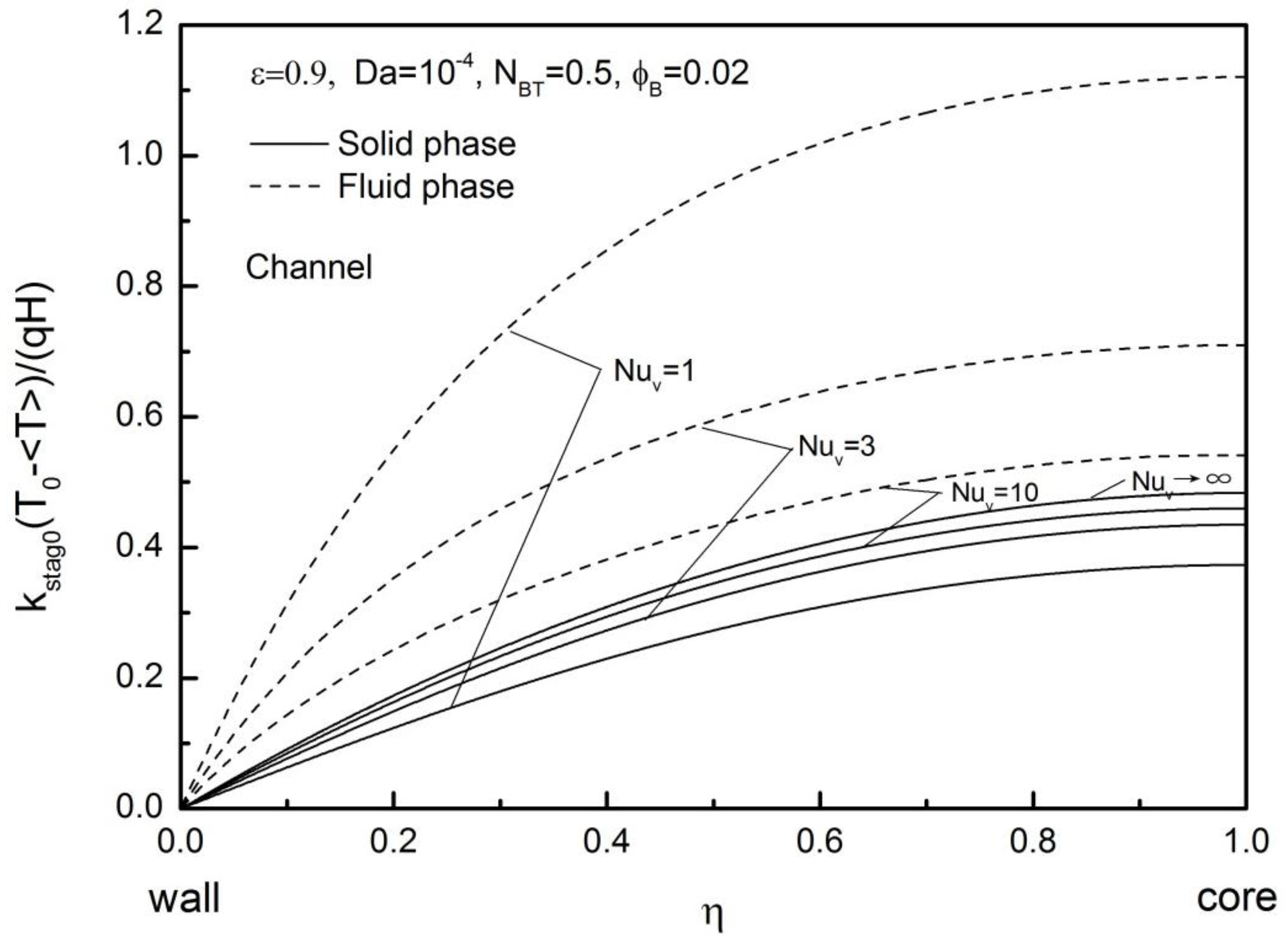
The foregoing set of equations may be integrated numerically using the Runge–Kutta–Gill method for the case of channel with $\epsilon$ = 0.9, $Da$ = 10⁻⁴, $N_{BT}$ = 0.5 and ${\varphi }_B$ = 0.02. Figure 12 shows the effects of the interstitial Nusselt number $N{u}_v$ on fluid and solid temperature profiles.

The temperature profile of nanofluid and that of metal foam tend to get closer each other for sufficiently large $N{u}_v$, in which local thermal equilibrium holds. Usually, the solid temperature is higher than the nanofluid temperature (i.e., $T{*}^s=k_{stag0}\left(T_0-{\langle T\rangle }^s\right)/q_{0}H$ is smaller and flatter than $T{*}^f=k_{stag0}(T_0-{\langle T\rangle }^f)/q_{0}H$).

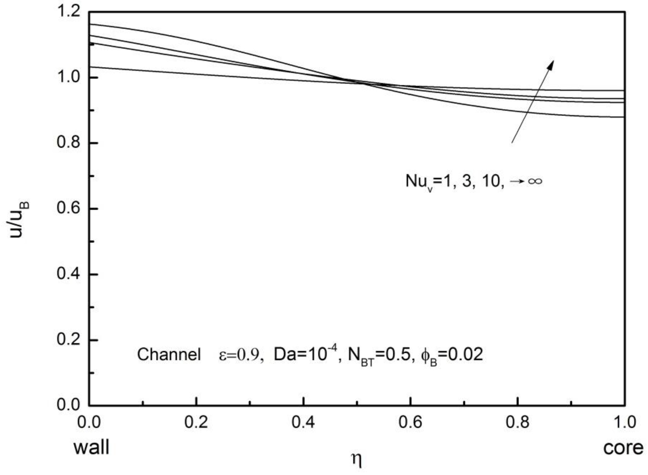
The corresponding particle volume fraction and velocity profiles in the channel are shown in Figure 13 and Figure 14, respectively. The nanoparticle volume fraction distribution becomes somewhat flatter as increasing $N{u}_v$, since the nanofluid temperature tends to follow the solid temperature, as witnessed in Figure 13. As can be seen from Figure 13, the nanoparticle volume fraction gradually converges to a profile corresponding to the case of $N{u}_v\to \infty$. Figure 14 clearly shows that the velocity is higher near the heated wall where viscosity is less, as thermophoretic diffusion dominates over Brownian diffusion, driving nanoparticles away from the wall.

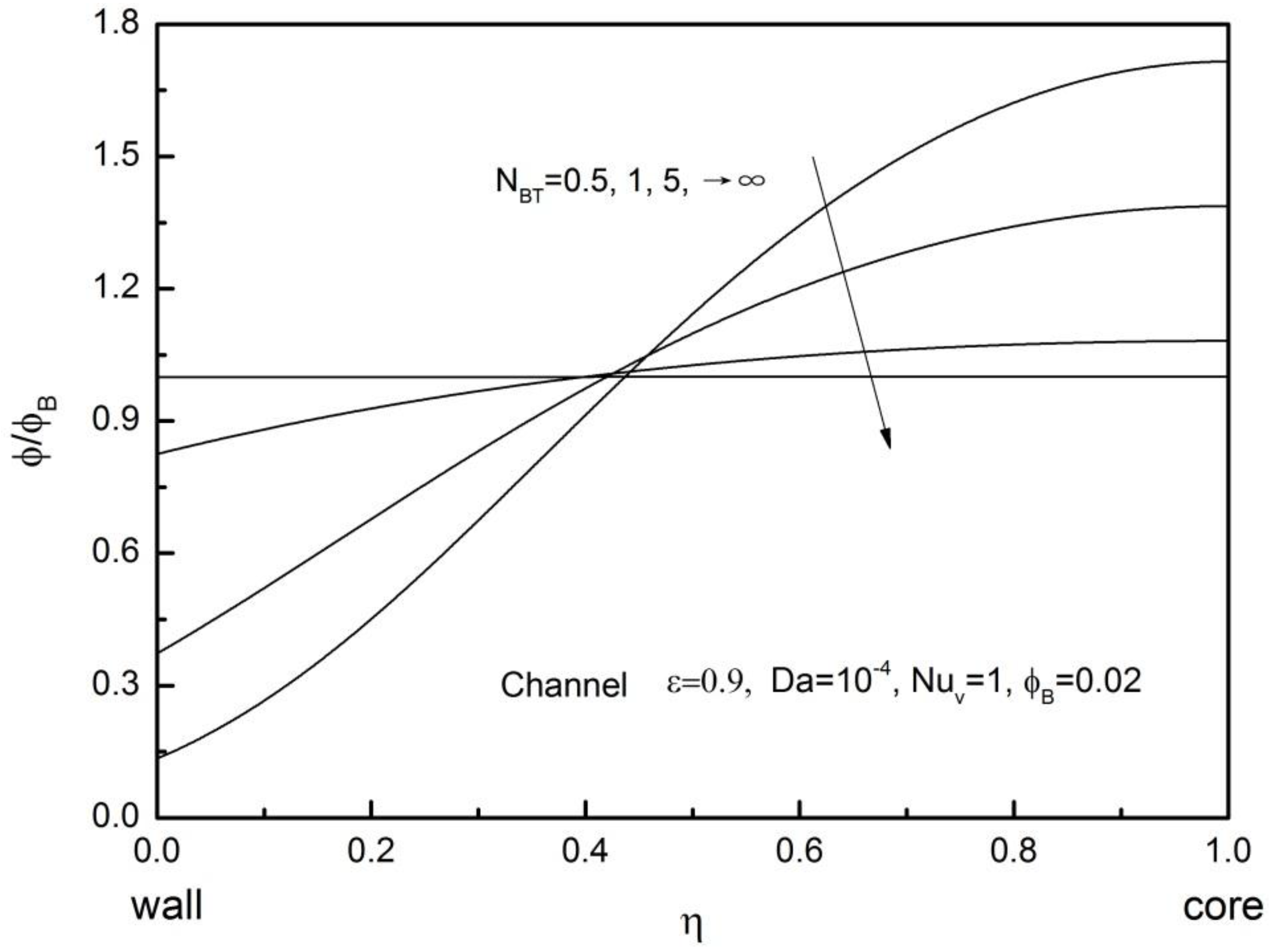
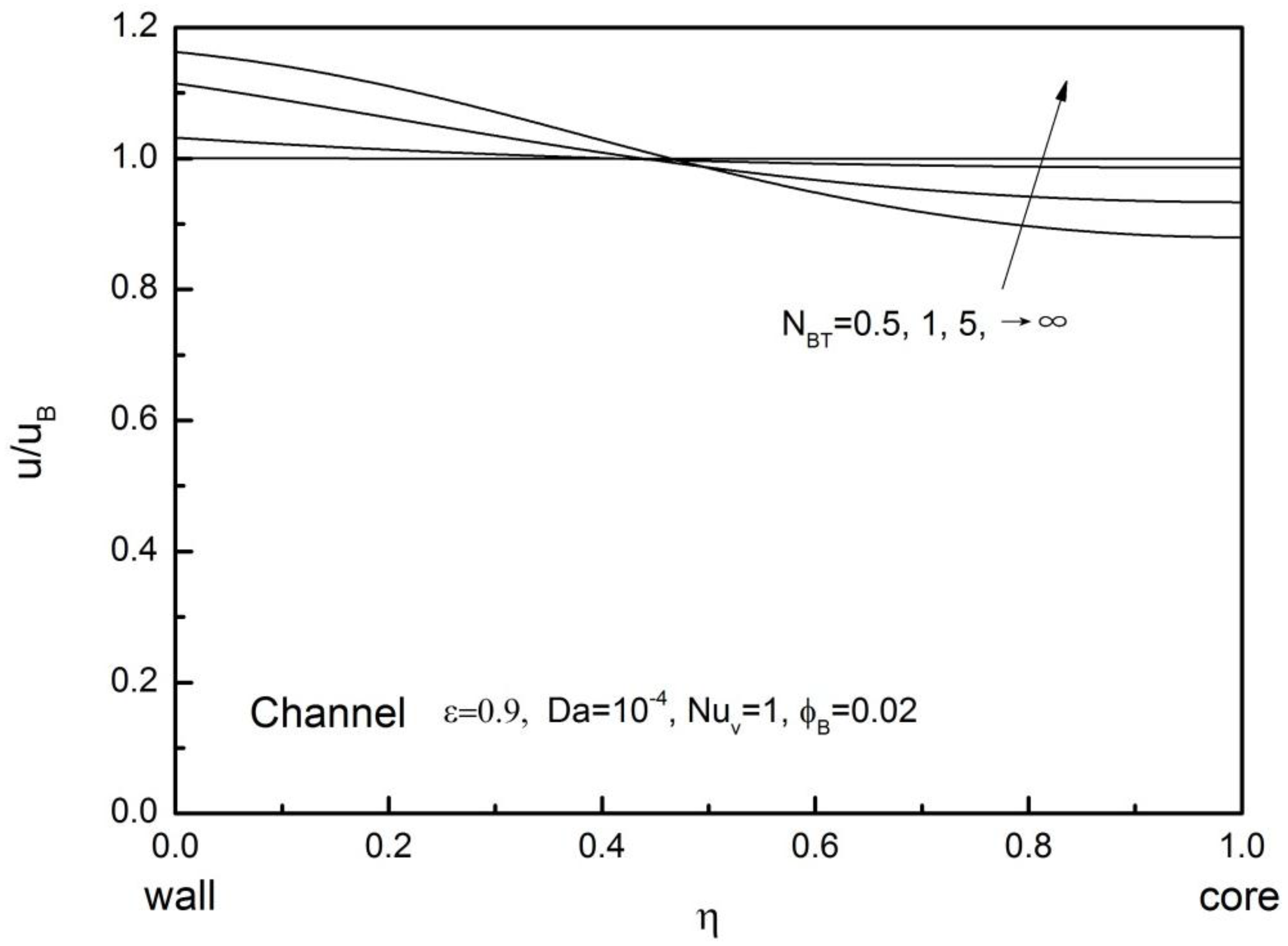
By changing the value $N_{BT}$, another series of computations were conducted with $\epsilon$ = 0.9, $Da$ = 10⁻⁴. $N{u}_v$ = 1 and ${\varphi }_B$ = 0.02, so as to investigate the effect of the ratio of macroscopic Brownian and thermophoretic diffusivities, $N_{BT}$, on nanoparticle volume fraction profile, velocity profile and both fluid and solid temperature profiles.

As shown in Figure 15, the nanoparticle volume fraction becomes uniform for large $N_{BT}$. Because Brownian diffusion dominates over thermophoretic diffusion, nanoparticles are dispersed evenly for large $N_{BT}$. Figure 16 shows that the velocity profile becomes completely flat under such a uniform nanoparticle volume fraction distribution, resulting in a plug flow.

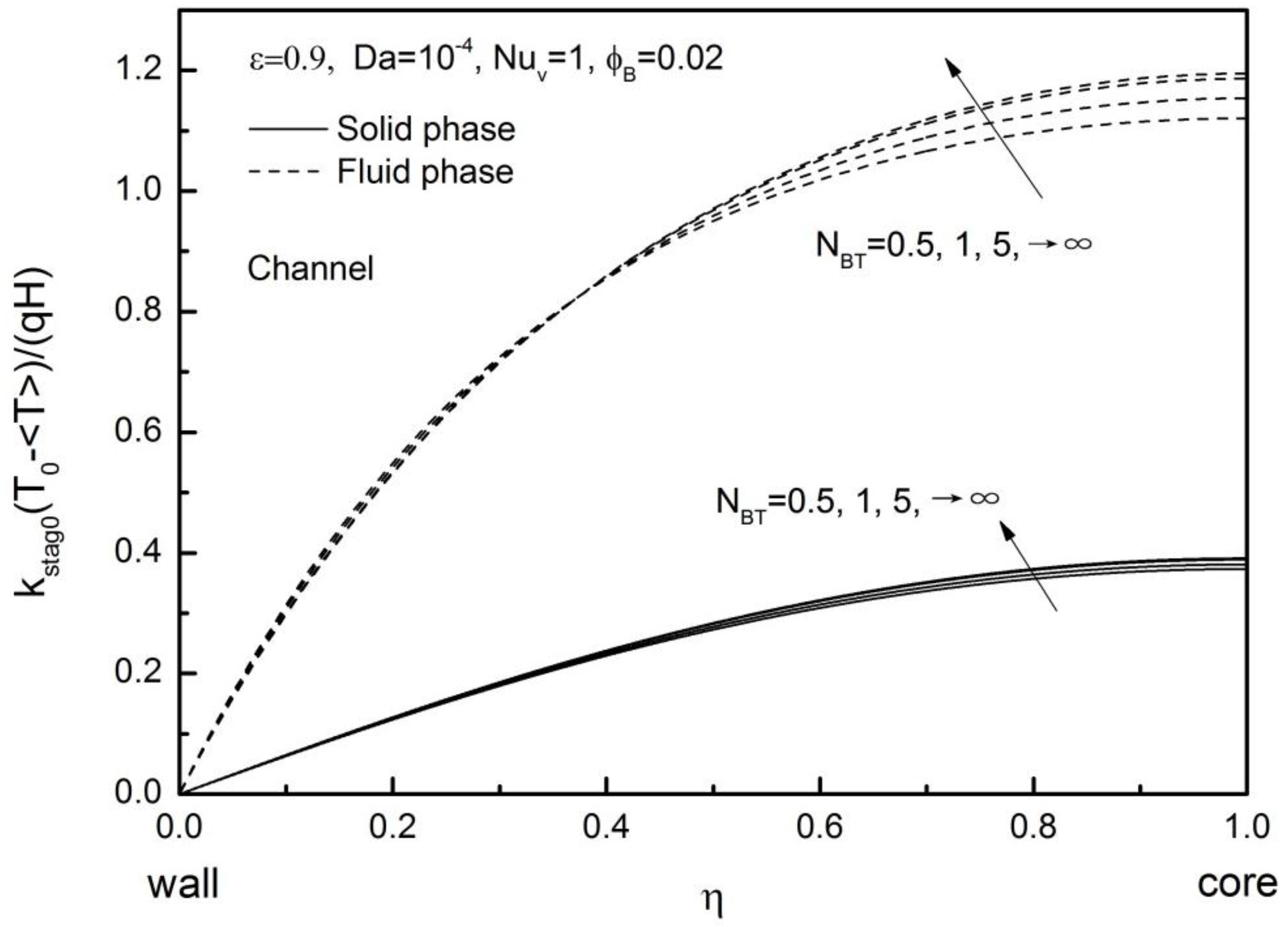
In Figure 17, both nanofluid temperature and metal foam temperature are plotted for a range of $N_{BT}$. $N{u}_v$ is only at a moderate level such that a substantial difference can be observed between two temperatures. As can be confirmed from the figure, however, the effects of $N_{BT}$ on the temperature profiles are rather limited.

9.1. Asymptotic Solutions for the Case of Nearly Uniform Nanoparticle Distribution ($N_{BT}>>1$)

Brownian diffusion overwhelms thermophoretic diffusion for the case of sufficiently small nanoparticle diameter, such that its macroscopic ratio $N_{BT}$ becomes much greater than unity. Equation (97) under such cases yields

$$\frac{{\langle \varphi \rangle }^f}{{\varphi }_0}=\exp \left(\frac{\epsilon *T{*}^f}{N_{BT}\epsilon \left(1-\gamma T{*}^f\right)}\right)\cong 1+\frac{\epsilon *}{N_{BT}\epsilon }T{*}^f$$

(102)

where $\gamma <<1$. The foregoing equation indicates that the profile of volume averaged nanoparticle volume fraction ${\langle \varphi \rangle }^f\left(y*\right)$ becomes similar to that of nanofluid phase temperature $T{*}^f\left(y*\right)$. Moreover, it tends to be uniform for sufficiently large $N_{BT}$, as consistently observed in Figure 15. Under such uniform distribution of volume averaged nanoparticle volume fraction, all thermophysical properties become uniform across the channel.

9.1.1. Channel Flows

Thus, the third order O.D.E. Equation (91) and nanofluid temperature Equation (96) with the boundary conditions Equations (98a) and (98b) yields the following analytic solutions:

$$T{*}^s=\frac{y*-\frac{1}{2}y{*}^2-\frac{1}{{\xi }^2}\left(1-\frac{\cosh \left(\xi \left(1-y*\right)\right)}{\cosh \xi }\right)}{1+{\zeta }_{k}Pe{u}_B*}$$

(103)

and

$$T{*}^f=\frac{y*-\frac{1}{2}y{*}^2+\frac{1-{\epsilon }^{*}\frac{k\left({\varphi }_B\right)}{k_{stag0}}}{\left({\epsilon }^{*}\frac{k\left({\varphi }_B\right)}{k_{stag0}}+{\zeta }_{k}Pe{u}_B^{*}\right){\xi }^2}\left(1-\frac{\cosh \left(\xi \left(1-y*\right)\right)}{\cosh \xi }\right)}{1+{\zeta }_{k}Pe{u}_B^{*}}$$

(104)

where

$$\xi =\sqrt{\frac{1+{\zeta }_{k}Pe{u}_B^{*}}{\left(1-{\epsilon }^{*}\right)\frac{k_s}{k_{stag0}}\left({\epsilon }^{*}\frac{k\left({\varphi }_B\right)}{k_{stag0}}+{\zeta }_{k}Pe{u}_B^{*}\right)}N{u}_v}$$

(105a)

and

$$u_B^{*}=\frac{\sqrt{1+4D{a}^{2}Hg}-1}{2DaHg}$$

(105b)

Nusselt number of our interest is given by

$$N{u}_H=\frac{q_{0}H}{k\left({\varphi }_B\right)\left(T_0-T_B\right)}=\frac{1}{\frac{k\left({\varphi }_B\right)}{k_{stag0}}{T}_B^{*}}=\frac{1}{\frac{k\left({\varphi }_B\right)}{k_{stag0}}\overline{T{*}^f}}=\frac{k_{stag0}}{k\left({\varphi }_B\right)}\frac{1+{\zeta }_{k}Pe{u}_B^{*}}{\frac{1}{3}+\frac{1-\frac{2+\epsilon }{3}\frac{k\left({\varphi }_B\right)}{k_{stag0}}}{\left(\frac{2+\epsilon }{3}\frac{k\left({\varphi }_B\right)}{k_{stag0}}+{\zeta }_{k}Pe{u}_B^{*}\right){\xi }^2}\left(1-\frac{\tanh \xi }{\xi }\right)}$$

(106)

The ratio of heat transfer coefficient for convection in a nanofluid saturated metal foam to that for the case of base fluid convection without a metal foam is given by

$$\frac{h\left({\varphi }_B\right)}{h_{bf}}=\frac{4}{\left(140/17\right)}\frac{k_{stag0}}{k_{bf}}\frac{1+{\zeta }_{k}Pe{u}_B^{*}}{\frac{1}{3}+\frac{1-\frac{2+\epsilon }{3}\frac{k\left({\varphi }_B\right)}{k_{stag0}}}{\left(\frac{2+\epsilon }{3}\frac{k\left({\varphi }_B\right)}{k_{stag0}}+{\zeta }_{k}Pe{u}_B^{*}\right){\xi }^2}\left(1-\frac{\tanh \xi }{\xi }\right)}$$

(107)

9.1.2. Tube Flows

The corresponding set of solutions for the case of tubes may be obtained by solving Equation (99) as

$$T{*}^s=\frac{y*-\frac{1}{2}y{*}^2-\frac{2}{{\xi }^2}\left(1-\frac{I_0\left(\xi \left(1-y*\right)\right)}{I_0\left(\xi \right)}\right)}{1+{\zeta }_{k}Pe{u}_B^{*}}$$

(108)

where $I_0$ is the modified zero order Bessel function of the first kind. The dimensionless nanofluid temperature is obtained substituting Equations (108) into (100) as

$$T{*}^f=\frac{y*-\frac{1}{2}y{*}^2+\frac{2\left(1-{\epsilon }^{*}\frac{k\left({\varphi }_B\right)}{k_{stag0}}\right)}{\left({\epsilon }^{*}\frac{k\left({\varphi }_B\right)}{k_{stag0}}+{\zeta }_{k}Pe{u}_B^{*}\right){\xi }^2}\left(1-\frac{I_0\left(\xi \left(1-y*\right)\right)}{I_0\left(\xi \right)}\right)}{1+{\zeta }_{k}Pe{u}_B^{*}}$$

(109)

where the dimensionless bulk velocity is given by Equation (105b). The corresponding Nusselt number may be numerically evaluated as

$$N{u}_R=\frac{q_{0}R}{k\left({\varphi }_B\right)\left(T_0-T_B\right)}=\frac{1}{\frac{k\left({\varphi }_B\right)}{k_{stag0}}{T}_B^{*}}=\frac{1}{\frac{k\left({\varphi }_B\right)}{k_{stag0}}\overline{T{*}^f}}$$

(110)

The ratio of heat transfer coefficient for convection in a nanofluid saturated metal foam to that for the case of base fluid convection without a metal foam is given by

$$\frac{h\left({\varphi }_B\right)}{h_{bf}}=\frac{2}{\left(48/11\right)}\frac{k_{stag0}}{k_{bf}}\frac{1}{\overline{T{*}^f}}$$

(111)

9.2. Asymptotic Solutions for the Case of Nearly Local Thermal Equilibrium ($N{u}_v>>1$)

Equation (96) for the channel flow case and Equation (100) for the tube flow case clearly indicate $T{*}^f\cong T{*}^s$ when the interstitial volumetric coefficient is sufficiently high (i.e., $N{u}_v>>1$). Thus, local thermal equilibrium holds everywhere over the cross-section.

9.2.1. Channel Flows

Equation (87) readily yields analytic solutions.

$$T{*}^f\cong T{*}^s={\displaystyle \underset{0}{\overset{y*}{\int }}\frac{{\displaystyle {\int }_{y*}^1\frac{\rho cu*}{\overline{\rho cu*}}dy*}}{\frac{k_{stag}}{{k_{stag}}_0}+{\zeta }_{k}Pe\left(\frac{\rho c}{{\rho }_0{c}_0}\right)u*}}dy*$$

(112)

This integral equation can be approximated very well by

$$T{*}^f\cong T{*}^s=\frac{y*-\frac{1}{2}y{*}^2}{\frac{k_{stag}\left({\varphi }_B\right)}{{k_{stag}}_0}+{\zeta }_{k}Pe\frac{\sqrt{1+4D{a}^{2}Hg}-1}{2DaHg}}$$

(113)

Substitution of the foregoing temperature profile into Equation (97) readily gives the profile of volume averaged nanoparticle volume fraction. The corresponding Nusselt number is given by

$$N{u}_H=\frac{q_{0}H}{k\left({\varphi }_B\right)\left(T_0-T_B\right)}=\frac{1}{\frac{k\left({\varphi }_B\right)}{k_{stag0}}{T}_B^{*}}=\frac{1}{\frac{k\left({\varphi }_B\right)}{k_{stag0}}\overline{T{*}^f}}=3\left(1+\frac{k_{stag0}}{k\left({\varphi }_B\right)}{\zeta }_{k}Pe\frac{\sqrt{1+4D{a}^{2}Hg}-1}{2DaHg}\right)$$

(114)

The ratio of heat transfer coefficient for convection in a nanofluid saturated metal foam to that for the case of base fluid convection without a metal foam is given by

$$\frac{h\left({\varphi }_B\right)}{h_{bf}}=\frac{12}{\left(140/17\right)}\left(\frac{k\left({\varphi }_B\right)}{k_{bf}}+\frac{k_{stag0}}{k_{bf}}{\zeta }_{k}Pe\frac{\sqrt{1+4D{a}^{2}Hg}-1}{2DaHg}\right)$$

(115)

9.2.2. Tube Flows

The corresponding set of the solutions for the case of tubes may be obtained from Equation (99) as

$$T{*}^f\cong T{*}^s={\displaystyle \underset{0}{\overset{y*}{\int }}\frac{{\displaystyle {\int }_{y*}^{1}2\left(1-y*\right)\frac{\rho cu*}{\overline{\rho cu*}}d\eta }}{\left(1-y*\right)\left(\frac{k_{stag}}{{k_{stag}}_0}+{\zeta }_{k}Pe\left(\frac{\rho c}{{\rho }_0{c}_0}\right)u*\right)}}dy*$$

(116)

which may well be approximated by

$$T{*}^f\cong T{*}^s=\frac{y*-\frac{1}{2}y{*}^2}{\frac{k_{stag}\left({\varphi }_B\right)}{{k_{stag}}_0}+{\zeta }_{k}Pe\frac{\sqrt{1+4D{a}^{2}Hg}-1}{2DaHg}}$$

(117)

Thus, the profile of volume averaged temperature given by Equation (117) and that of nanoparticle volume fraction given by its substitution into Equation (97) for the tube are similar to those for the channel. Accordingly, Nusselt number for the tube is given by

$$N{u}_R=\frac{q_{0}R}{k\left({\varphi }_B\right)\left(T_0-T_B\right)}=\frac{1}{\frac{k\left({\varphi }_B\right)}{k_{stag0}}{T}_B^{*}}=\frac{1}{\frac{k\left({\varphi }_B\right)}{k_{stag0}}\overline{T{*}^f}}=4\left(1+\frac{k_{stag0}}{k\left({\varphi }_B\right)}{\zeta }_{k}Pe\frac{\sqrt{1+4D{a}^{2}Hg}-1}{2DaHg}\right)$$

(118)

The ratio of heat transfer coefficient for convection in a nanofluid saturated metal foam to that for the case of base fluid convection without a metal foam is given by

$$\frac{h\left({\varphi }_B\right)}{h_{bf}}=\frac{8}{\left(48/11\right)}\left(\frac{k_{stag}\left({\varphi }_B\right)}{k_{bf}}+\frac{k_{stag0}}{k_{bf}}{\zeta }_{k}Pe\frac{\sqrt{1+4D{a}^{2}Hg}-1}{2DaHg}\right)$$

(119)

Heat transfer enhancement in a nanoparticle saturated metal foam can be partly due to an increase in its stagnant thermal conductivity, which results from both highly conductive nanoparticles and consolidated meal foam, and partly due to intensified nanofluid mixing resulting from mechanical dispersion within a foam. This enhancement can best be illustrated in the foregoing Equation (119). The first term in the right hand side gives the heat transfer rate increase due to embedding of metal foam and addition of nanoparticles, while the second term describes heat transfer enhancement due to thermal dispersion.

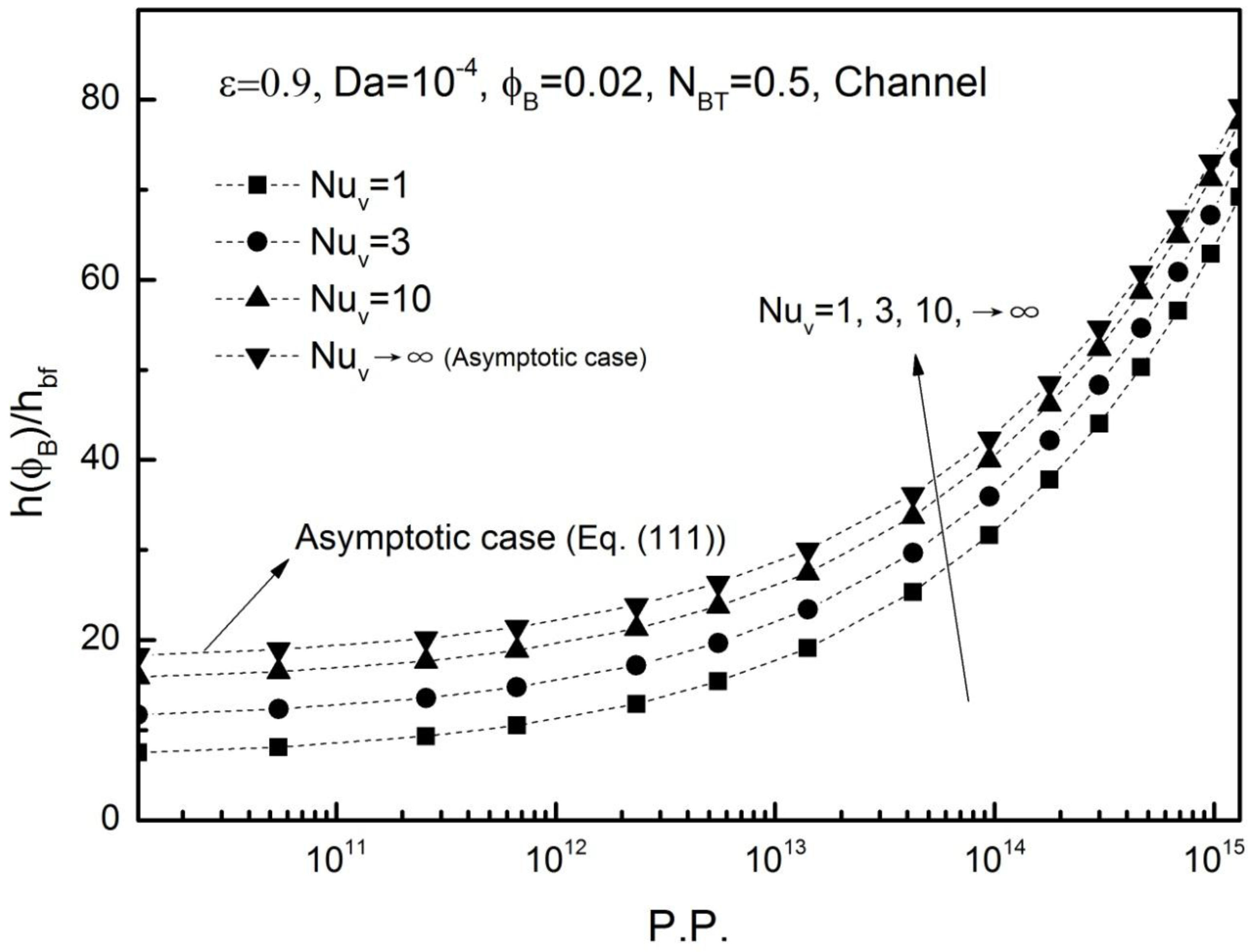
9.3. Heat Transfer Performance Evaluation

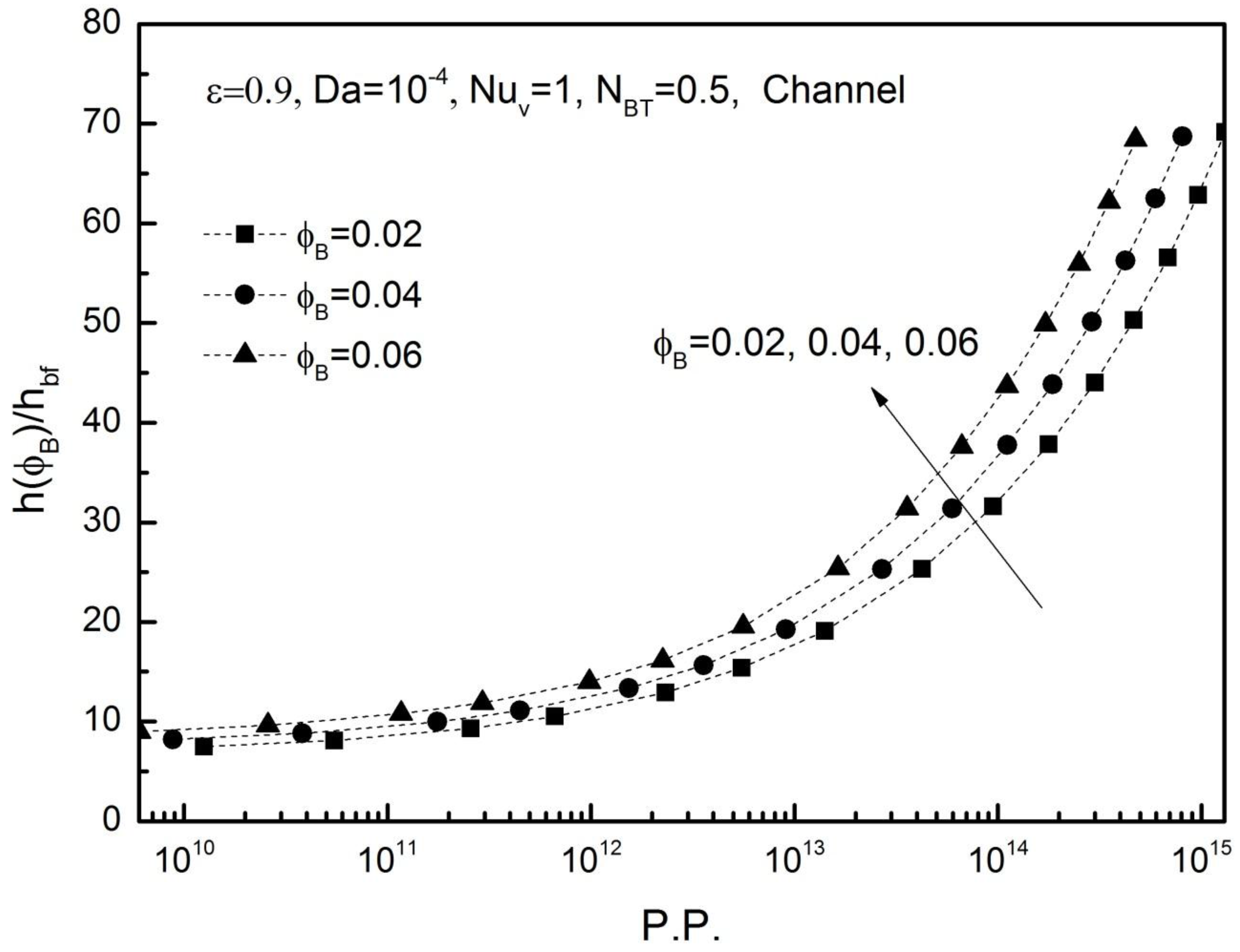
Figure 18 shows heat transfer coefficient ratios $h\left({\mathsf{\phi }}_B\right)/h_{bf}$ for given ${\varphi }_B$ against a dimensionless pumping power:

$$P.P.\left(Hg;Da\right)\equiv \left(-\frac{d{\langle p\rangle }^f}{dx}{u}_B\right)\left(\frac{{{\rho }_0}^2{b}^2{R}^6}{{{\mu }_0}^3}\right)=\frac{\sqrt{1+4D{a}^{2}Hg}-1}{2Da}Hg$$

(120)

$h\left({\varphi }_B\right)/h_{bf}$ is plotted in a possible range of P.P. = 6.0 × 10⁹ − 1.3 × 10¹⁵ (corresponding to $\langle u\rangle$= 0.01 to 1 m/s, 2R = 0.02 m, $d_m$ = 0.001 m) for the tube. The figure clearly indicates that heat transfer coefficient for the tube filled with a nanofluid saturated metal foam is much higher than that for a tube filled with a base fluid. The ratio increases towards 80 as increasing the pumping power $P.P.$, in which thermal dispersion becomes significant. Naturally, higher volume fraction of nanofluid results in higher heat transfer coefficient, especially when $P.P.$ is large such that thermal dispersion is quite significant.

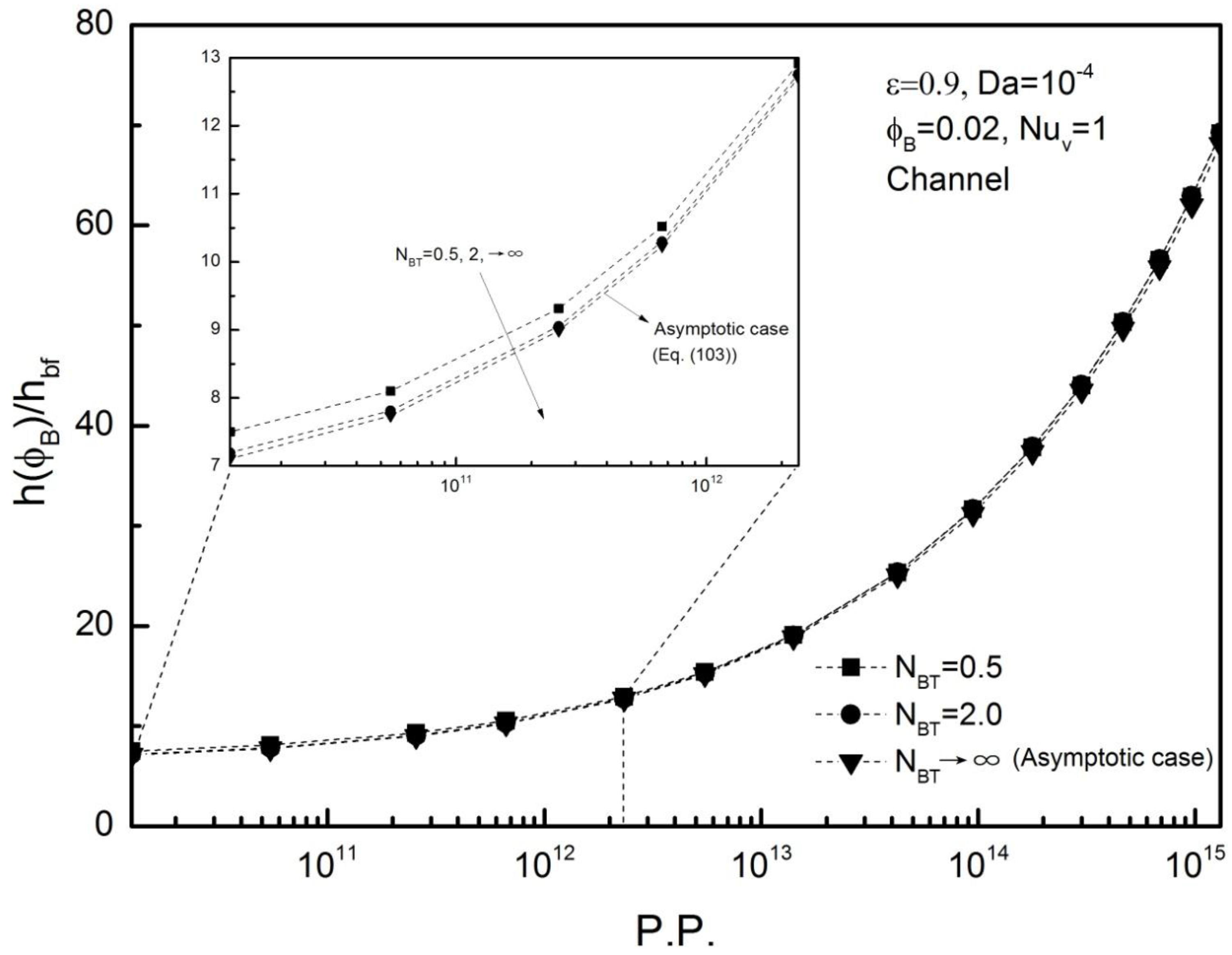
Figure 19 shows the effects of $N_{BT}$ on the heat transfer ratio $h\left({\varphi }_B\right)/h_{bf}$. As expected from Figure 17 showing the temperature profiles, which are fairly insensitive to $N_{BT}$, the heat transfer ratios obtained with different values of $N_{BT}$ almost coincide one another. Figure 20, on the other hand, shows effects of $N{u}_v$ on the heat transfer coefficient ratio $h\left({\varphi }_B\right)/h_{bf}$, which clearly indicates that higher interstitial heat transfer coefficient yields higher macroscopic heat transfer coefficient. Therefore, combination of metal foams and nanofluids is believed to bring unconventionally high heat transfer coefficients.

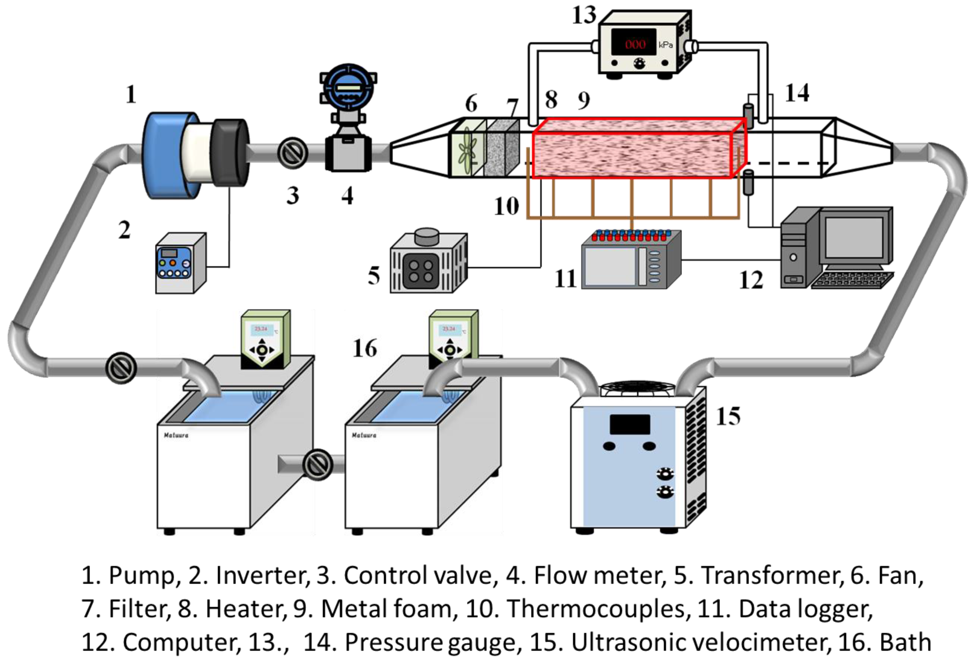
The experimental verification is underway using the experimental set-up, as shown in Figure 21. The experimental results obtained from the program partially supported by the JSPS Grants-in-Aid for Scientific Research B, will be available near future.

10. Concluding Remarks

A rigorous derivation of the macroscopic governing equations was presented for analyzing convective heat transfer in nanofluid saturated metal foam. A volume averaging theory was introduced to integrate the microscopic set of the modified Buongiorno equations over a local control volume. The unknown correlation terms resulting from the volume averaging were mathematically modeled so as to close the set of governing equations. A pore scale conduit model was used to investigate both thermal dispersion term and particle mechanical dispersion term analytically. Upon assuming microscopic distribution profiles for velocity and temperature within a pore, dispersion coefficients were evaluated for thermal dispersion and particle mechanical dispersion. The present analytical expression for the transverse thermal dispersion based on the pore scale analysis was found to closely follow the Calmid–Mahajan empirical correlation. The longitudinal particle mechanical dispersion was found to work either to suppress or to enhance effective diffusion depending on the sign of local phase temperature difference, while the transverse counterpart is insignificant and therefore can be neglected. Moreover, it has been found, conducting a comparison under equal pumping power, that a high level of the heat transfer rate (about 80 times more than the case of base fluid convection without a metal foam) is possible using a combination of metal foam and nanofluid. Thus, we can conclude that the nanofluid saturated metal foams can be utilized for conceiving a new generation of high performance heat exchangers.

It should finally be pointed out that possible nanofluid fouling due to nanoparticles coagulation on the internal wall of solid matrix has been neglected in this study. Sarafraz et al. [41] conducted experiments to investigate the role of nanofluid fouling on thermal performance of a thermosiphon, and pointed out that the form of the deposited layer can be affected by nanofluid concentration, applied heat load, inclination of thermosiphon and operation time. Their experimental data clearly indicate that the existence of the deposited layer increases the thermal resistance, deteriorating heat transfer performance. Naturally, more power loss is expected since the deposited layer blocks the transport path of nanofluid.