A Framework for Classifying Movie Networks Using Graph Neural Networks

Abstract

Movie genre classification is a significant challenge in narrative analysis, as traditional methods often fail to capture complex structural relationships within movie stories. This study introduces the Intra-Cluster Weighted Movie Network (ICWMN), a novel framework designed to improve classification by using intra-movie relationships through Graph Neural Networks (GNNs). We constructed a large-scale dataset of 1631 movie character networks using an automated pipeline comprising web scraping, regular expressions, and fine-tuned BERT models for entity recognition. To address the computational limitations of fully connected models, we partition ICWMN into clusters and establish edges only between the k-most similar nodes using the K-Nearest Neighbor algorithm and various distance measures, such as the Laplacian and NetLSD. XGBoost is applied to optimize high-dimensional node feature vectors. Experimental results demonstrate outstanding performance, with the Graph Attention Network (GAT) emerging as the top-performing architecture, resulting in classification accuracies that peak at $95.00\%$ on our 1631-movie dataset and an exceptional $97.30\%$ on the 773-movie Moviegalaxies dataset. These findings confirm that prioritizing spectral properties and cluster-based network topologies significantly improve the precision and stability of genre classification compared to state-of-the-art methods.

1. Introduction

Movie genre classification remains a significant challenge in the study of complex networks and narrative analysis. Traditional movie classification methods have focused mainly on extracting features from data sources, such as audio-visual characteristics [1], scene categorization [2], metadata from poster images [3], convolutional neural networks [4], and recurrent neural networks [5]. However, all of these approaches ignore the structural relationships within movies.

Graphs are non-Euclidean data structures that represent a set of entities as nodes and their interactions as edges. The application of graph theory to movie analysis has emerged as a significant trend, representing a complex area within the study of complex networks. Chakrabarti et al. [6] were among the first to employ graphs for node classification by defining the problem as a supervised classification task that models hypertexts as graphs. Zhu and Ghahramani [7] employ graphs for node classification by defining the problem as a semi-supervised learning task and using the label propagation algorithm. Machine learning approaches are classified into supervised and unsupervised. Supervised learning focuses on finding the relationships between input features and a target variable, while unsupervised learning aims to identify patterns and extract characteristics from unlabeled data. Traditional machine learning algorithms typically treat each node as an independent data point, relying only on node attributes and neglecting the structural relationships among nodes. Network embedding methods, such as DeepWalk [8] and node2vec [9], generate low-dimensional vector representations for nodes, which can subsequently operate as input for conventional classifiers, including support vector machines (SVM). Nonetheless, the majority of embedding-based approaches operate in a transductive manner, limiting their ability to generalize to new or previously unseen nodes without retraining the entire model.

Bruna et al. [10] were among the first to extend convolutions—which performed so well for images—to graphs. They used the graph Laplacian and the Fourier domain to define graph convolutions. Graph neural networks (GNNs) are engineered to process graph-structured data. Over the past decade, a substantial number of GNN subcategories have been introduced in response to the challenges associated with learning from graphs. Graph Convolutional Networks (GCNs) [11] represent a semi-supervised, transductive learning model that employs convolutional operations adapted for graph data to extract features from node neighborhoods. GraphSAGE [12] is an inductive learning framework that generates node embeddings by sampling and aggregating information from the neighbors of each node, thereby enabling the model to generalize to previously unseen nodes. Graph Attention Networks (GATs) [13] incorporate the attention mechanism into the GNN architecture, allowing for the dynamic weighting of neighboring nodes’ contributions during the aggregation process.

In the literature, movie genre classification has been widely investigated using various machine learning techniques applied to diverse data forms. Several approaches rely on textual and narrative structures extracted from scripts or subtitles. Kagan et al. [14] designed the Subs2Network framework, which uses natural language processing (NLP) and named-entity recognition (NER) to map out character networks from movie subtitles. Instead of standard genre mapping, their work evaluates gender representation and relationship evolution over time, training classifiers on a mix of graph metrics (vertex and network features) and movie metadata to predict if a character network passes the Bechdel test. Idem, relying on text, Fei and Zhang [15] used TF-IDF scores to isolate highly descriptive words from movie documentation, mapping these key terms directly to specific genres using a Support Vector Machine (SVM).

Other research has focused heavily on multimedia and audio-visual cues. Huang and Wang [16] combined high-level video elements with acoustic features, passing them through an SVM classifier to categorize genres. Beyond video and text, visual metadata from promotional material has also been explored. Simões et al. [4] introduced CNN-MoTion, a multi-classification framework that integrated convolutional neural networks to extract both low-level and high-level video characteristics alongside audio features. Sorratat and Panita [17] proposed the SEMPD framework to extract semantic features from movie posters—including design layout, color profiles, and emotional themes—and handled classification via multi-label algorithms such as MLkNN and Classifier Chains.

While these methodologies exploit audio, video, textual, or poster-based attributes, they largely treat movies as isolated multimedia blocks. Even when character interactions are modeled, existing frameworks rarely use pure structural network topologies for explicit genre classification.

For this, we have proposed in [18] an approach to classify movie genres by extracting features from character networks constructed from movies in the Movie Galaxy dataset. Character network construction captures the interaction patterns between characters. The feature vector was created by combining thirteen network properties, which we categorized as statistical, spectral, and embedding features. These features were evaluated using four machine learning classifiers: Random Forest (RFC), Support Vector Machines (SVM/SVC), and Gaussian Process Classifiers (GPC). The results demonstrated that SVM and GPC classifiers achieved the best accuracy, with an ablation study further indicating the strong influence of statistical network features in the identification of movie genres.

Although several methodologies have successfully tackled movie genre classification, the integration of Graph Neural Networks (GNNs) in this domain remains largely novel. Huang and Wang [16] combined multimodal trailer features with feature selection techniques to achieve an SVM classification accuracy of 91.9%. Perri et al. [19] showcased the strength of graph-based deep learning by successfully applying GNNs to characterize networks within J.R.R. Tolkien’s fictional universe. Simões et al. [4] utilized a CNN-based framework to analyze frame-level details from movie trailers. However, for actual movie genre tasks, Mizvol [20] applied standard machine learning to character networks, but struggled to cross a 59% accuracy threshold.

Although these studies demonstrate that network structures provide valuable information, they all share a common limitation: each movie or character network is treated as an isolated entity, ignoring the connections between different movies, leading to a low accuracy.

To address this limitation, we formulate the problem as a node classification task, where each movie is represented as a node. This approach allows us to exploit the structural relationships between different movies. By exploiting the power of Graph Neural Networks (GNNs), the model aggregates information from neighboring nodes, combining both node features and relationships to improve classification performance.

We then proposed a (GNN)-based approach [21] for movie genre classification, which addresses the limitations of traditional methods by exploiting inter-movie relationships. We constructed a Fully Connected Weighted Movie Network (FCWMN), where each movie is represented as a node associated with a feature vector that integrates statistical, embedding, and spectral network properties derived from its character network. The connections in the FCWMN are weighted using the Network Portrait Divergence [22] to quantify the similarity between character networks, ensuring that similar movies have stronger links. Subsequently, a graph convolutional network (GCN) is applied for node classification, which aggregates features and relational information from neighboring nodes, leading to a classification accuracy of 87% when combining statistical and spectral features.

A significant limitation of the FCWMN appears when scaling to large networks comprising millions of edges. Because GNN architectures rely on propagating messages between connected nodes, the computational cost becomes excessive as the number of edges increases, causing the model to fail.

The main contributions of this work are as follows:

• We constructed a large dataset comprising 1631 movie character networks by automatically extracting and processing scripts from public repositories. Our approach integrates web-scraping techniques, regular expression, and fine-tuned transformer models (BERT) to accurately identify character names, even in unstructured scripts. Each script is then represented as a weighted undirected graph in which nodes correspond to characters, and edge weights indicate the frequency of their interactions within scenes.
• We address the challenge of FCWMN by reducing the number of edges. We partition the movie network into clusters where an edge is established only between a node i and its k most similar nodes. Neighbor selection was implemented via the algorithm K-Nearest Neighbor (K-NN), where similarity between nodes is determined by a distance measure such as the Laplacian, the NetLSD [23], and the Network Portrait Divergence [22]. As a result, we constructed three Intra-Cluster Weighted Movie Networks (ICWMN), each based on connections defined by one of these distance measures.
• We conducted an exhaustive evaluation of the ICWMN, assessing the classification performance of graph neural network models, such as GAT, GCN, and GraphSAGE. This comparative framework aims to identify the optimal architecture of graph neural networks and the distance measure that most effectively exploit ICWMN to achieve high genre classification accuracy.

The rest of this paper is structured as follows: Section 2 provides a comprehensive background on distance measures, graph neural networks, and feature selection algorithms. Section 3 represents the proposed method for constructing the character network database, ICWMN, and the movie node classification architecture. Section 4 presents the experimental evaluation and a detailed discussion of the results. Finally, we conclude in Section 5.

2. Background

Before introducing ICWMN, we review background knowledge on distance measures (Section 2.1) and graph neural networks (Section 2.2).

2.1. Graph Distances

In [24], we established a methodology to quantify the similarity of movie stories based on two main components. First, we incorporated various elements of the movie story, including characters, keywords, and locations. Second, we calculate the distance between the respective movie networks employing five different graph distance measures. We further investigated methods to determine the relative similarity among movies within a specific genre and to classify movie stories according to their genre. The approach used a multilayer network model [25] to represent the elements of movie stories. The analysis mainly focused on comparing monolayers of the same entities, without considering inter-relationships.

As we work on graphs where node correspondence is unknown, we have evaluated distances across spectral, embedding, and statistical approaches—specifically Network Matrix Factorization (NetMF) [26], Network Laplacian Spectra Descriptor (NetLSD) [23], Laplacian Spectra, Portrait Divergence [22], and the D-measure [27]. Our findings indicate that the effectiveness of an approach depends heavily on the network’s topology and the measure’s ability to capture those structures. For instance, we found that Network Portrait Divergence and NetLSD are effective for comparing character layers (typically small-world graphs). In contrast, the Laplacian spectral approach proved most effective for comparing keyword and location layers, which tend to exhibit scale-free and chain-like structures. Results for NetMF and D-measure, however, remained ambiguous. In the present work, we employ the NetLSD, the Portrait Divergence, and the Laplacian to construct the ICWMN.

The process of computing the distance between a couple of graphs proceeds in two main stages: (i) the extraction of a network property or a vector of properties, and (ii) the computation of the distance between them. This section provides a concise overview of the three distance measures.

2.1.1. Network Laplacian Spectral Descriptor (NetLSD)

NetLSD [23] is network property that captures the structural signature of a network based on heat diffusion features. NetLSD derives an n-dimensional vector $u_t$ from the heat equation ${\displaystyle \frac{\partial u_t}{\partial t}}=-\tilde{\mathcal{L}}{u}_t$, where $u_t$ represents the heat properties of the nodes over time t. The closed-form solution to this equation is the $n\times n$ heat kernel matrix $H_t$, defined as:

$$H_t=e^{-t\tilde{\mathcal{L}}}=\mathrm{\Phi }{e}^{-t\mathrm{\Lambda }}{\mathrm{\Phi }}^{\top }$$

(1)

where $\tilde{\mathcal{L}}$ is the normalized Laplacian, $\mathrm{\Phi }$ is the matrix of its eigenvectors, and $e^{-t\mathrm{\Lambda }}$ is the diagonal matrix of exponentiated eigenvalues. The heat matrix $h_t$ verifies three properties: permutation-invariance, scale-adaptive, and size-invariant.

2.1.2. Laplacian Spectra

The Laplacian spectra serves as a robust metric for network characterization due to its inherent properties of permutation invariance and scale adaptivity. Using the spectral signature, the structural similarity between two networks can be quantified by calculating the Euclidean distance between their respective sets of eigenvalues, such as:

$$dist({\int }_{{\mathcal{G}}_A},{\int }_{{\mathcal{G}}_B})=\sqrt{\sum _{i=1}^n{({\lambda }_{A_i}-{\lambda }_{B_i})}^2}$$

(2)

where ${\int }_{{\mathcal{G}}_A}=({\lambda }_{A_1},{\lambda }_{A_2},\dots ,{\lambda }_{A_n})$ and ${\int }_{{\mathcal{G}}_B}=({\lambda }_{B_1},{\lambda }_{B_2},\dots ,{\lambda }_{B_n})$ represent the spectral vectors of graphs ${\mathcal{G}}_A$ and ${\mathcal{G}}_B$, respectively.

2.1.3. Portrait Divergence

Portrait Divergence [22] is a permutation-invariant metric designed for the structural comparison of complex networks. This approach characterizes a graph through its Network Portrait [28], which is a matrix $\mathcal{B}$ representing the distribution of distances between nodes. Each row in $\mathcal{B}$ corresponds to the probability distribution $\pi \left(k\right|l)$, defined as:

$$\pi \left(k\right|l)={\displaystyle \frac{1}{N}}{\mathcal{B}}_{l,k}$$

(3)

where k denotes the number of vertices reachable at a distance l from a randomly selected node.The computation of the divergence between two networks, ${\mathcal{G}}_A$ and ${\mathcal{G}}_B$, follows a two-stage process. First, the respective probability distributions ${\pi }_{{\mathcal{B}}_A}$ and ${\pi }_{{\mathcal{B}}_B}$ are derived for each graph. Second, the topological distance between the portraits ${\mathcal{B}}_A$ and ${\mathcal{B}}_B$ is quantified using the Jensen-Shannon ($dis{t}_{JS}$) divergence:

$$D_{JS}({\mathcal{G}}_A,{\mathcal{G}}_B)={\displaystyle \frac{1}{2}}\left(KL({\pi }_{{\mathcal{B}}_A}\Vert \pi )+KL({\pi }_{{\mathcal{B}}_B}\Vert \pi )\right)$$

(4)

where ${\pi }_{*}={\displaystyle \frac{1}{2}}({\pi }_{{\mathcal{B}}_A}+{\pi }_{{\mathcal{B}}_B})$ represents the mixture distribution and the term $KL(·\Vert ·)$ denotes the Kullback–Leibler (K) divergence.

2.2. Graph Neural Networks

Graph neural networks learn node representations and the relationships between nodes by aggregating information from neighbors in a multi-layered process. This is accomplished through the message passing step.

2.2.1. Message Passing

Message passing, introduced by Gilmer et al. [29], process at each layer following three main steps: message construction, message aggregation, and node update. A message passing layer is computed as follows:

$$h_i^{(l+1)}=\varphi \left(h_i^{\left(l\right)},\underset{j\in \mathcal{N}\left(v_i\right)}{⨁}\psi \left(h_i^{\left(l\right)},h_j^{\left(l\right)}\right)\right)$$

(5)

where ⨁ denotes an aggregation operator, which may include functions such as sum, max, or mean. The function $\psi$ creates a message from neighbor j to the target node i, capturing the relevant information from node j to node i. The update function $\varphi$ then takes as input the current feature vector of node $h{i}^{\left(l\right)}$, along with the aggregated messages from all its neighbors, ${⨁}_{j\in \mathcal{N}\left(v_i\right)}\psi \left(h_i^{\left(l\right)},h_j^{\left(l\right)}\right)$, to produce the updated node representation $h_i^{(l+1)}$ at layer $l+1$.

2.2.2. Graph Attention Networks (GAT)

The Graph Attention Network (GAT), introduced by Veličković et al. [13] in 2018, uses an inductive learning approach rather than relying on a predefined function. A key component of the GAT architecture is the self-attention mechanism, which computes the learned weight $a_{v_i{v}_j}$ (Equation (6)) that explicitly indicates the importance of a neighbor $v_j$ to a node $v_i$ during the aggregation process.

$${\alpha }_{v_i{v}_j}=softmax\left(e_{v_i{v}_j}\right)={\displaystyle \frac{exp\left(e_{v_i{v}_j}\right)}{{\sum }_{k\in {\mathcal{N}}_i}exp\left(e_{v_i{v}_k}\right)}}$$

(6)

The computation of attention coefficients is performed in parallel across all edges, and the subsequent aggregation is performed in parallel across all nodes, allowing the model to capture diverse neighborhood relationships. The resulting aggregation feature ${\mathcal{X}}_i^{\prime }$ for a single attention head $\mathbf{H}$ = 1 is presented in Equation (7).

$${\mathcal{X}}_i^{\prime \left(l\right)}=\sigma \left(\sum _{j\in {\mathcal{N}}_i}{a}_{v_i{v}_j}^{(l-1)}{\mathbf{W}}^{(l-1)}{x}_{v_j}\right)$$

(7)

For multihead $\mathbf{H}$ = $\left(1,2,...,h\right)$, the resulting aggregated features are combined, typically via concatenation $(\Vert )$ as defined by Equation (8).

$${\mathcal{X}}_i^{\prime }{=\Vert }_{h=1}^{\mathbf{H}}\sigma \left(\sum _{j\in {\mathcal{N}}_i}{a}_{v_i{v}_j}^h{\mathbf{W}}^h{x}_{v_j}\right)$$

(8)

where $\sigma$ denotes the activation function, $\mathbf{A}$ represents the adjacency matrix, and ${\mathbf{W}}^{\left(l\right)}$ is the trainable weight matrix.

2.2.3. Graph Convolution Networks (GCN)

The Graph Convolutional Network (GCN), a transductive learning method introduced by Kipf and Welling in 2016 [11], offers a computationally efficient framework for applying convolutional neural networks (CNNs) [30] to graph-structured data. The primary objective of the GCN is to iteratively refine node features by aggregating information from neighboring nodes. In each convolutional layer l, the features of the nodes are reviewed by aggregating the features of the adjacent nodes, resulting in the updated feature matrix ${\mathcal{X}}^{\prime \left(l\right)}$ (see Equation (9)).

$${\mathcal{X}}^{\prime \left(l\right)}=\sigma \left({\Delta }^{-1/2}\mathbf{A}{\Delta }^{-1/2}{\mathcal{X}}^{(l-1)}{\mathbf{W}}^{(l-1)}\right)$$

(9)

where $\Delta$ represents the degree matrix.

2.2.4. Graph Sample and Aggregate (GraphSAGE)

Introduced by Hamilton in 2017 [12], GraphSAGE is an inductive learning approach for creating node representations in large-scale graph environments. The methodology for updating node features implies aggregating data from adjacent nodes, similar to Graph Convolutional Networks (GCNs). Particularly, GraphSAGE differentiates itself by learning a generalizable aggregation function without resorting to a predetermined function, enabling the model to generate embeddings for unseen nodes without necessitating a complete retraining cycle. The framework applies varying aggregation functions in different computational layers (Equation (10)).

$${\mathcal{X}}^{\prime \left(l\right)}=\sigma \left({\mathbf{W}}^{\left(l\right)}·\mathrm{CONCAT}\left({\mathcal{X}}^{(l-1)},{\mathcal{AGG}}^{\left(l\right)}\left({\mathcal{X}}^{(l-1)}\right)\right)\right)$$

(10)

where $\mathcal{AGG}$ is an aggregation function.

3. Proposed Method

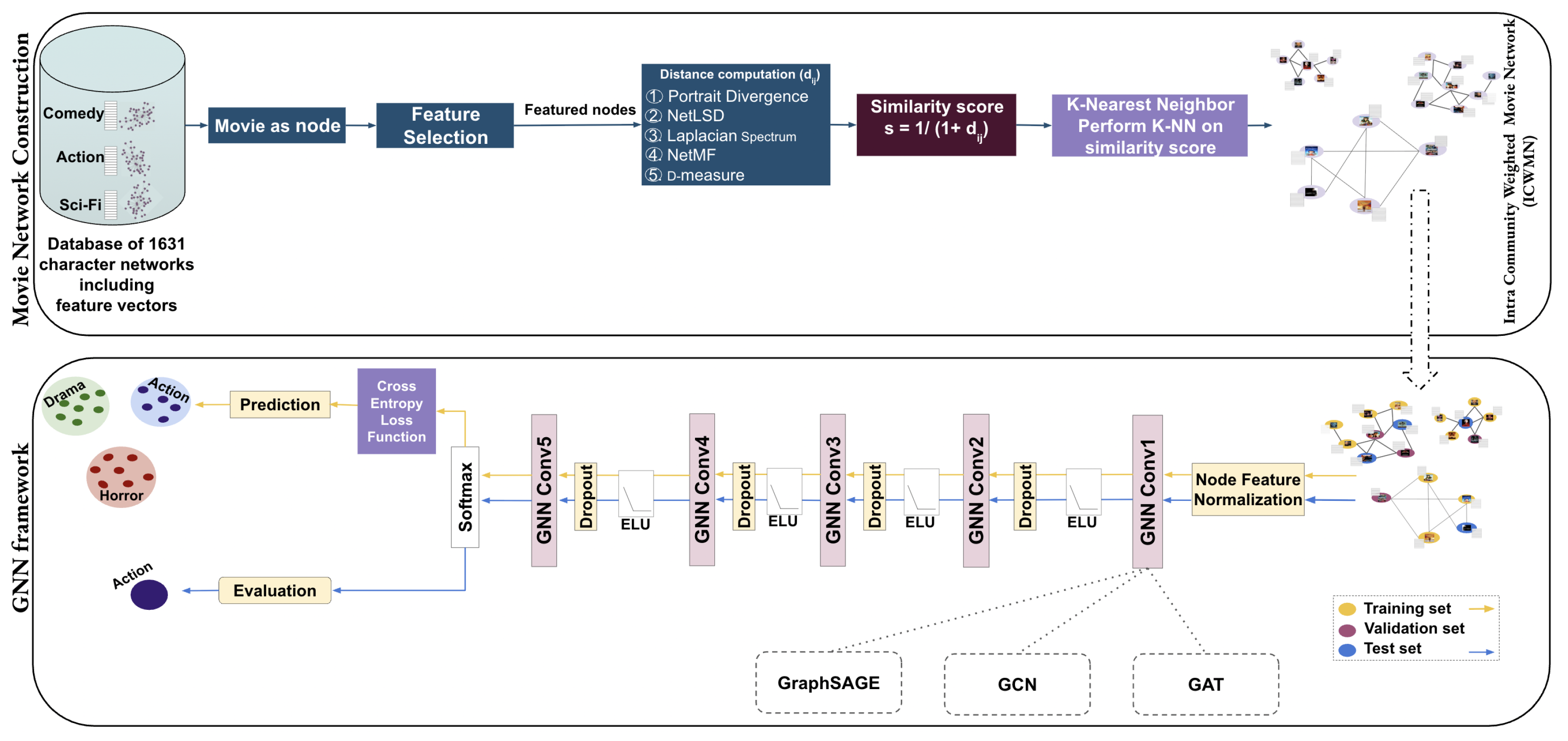
In this work, we present a novel framework for movie genre classification founded on graph neural networks, distance measures, and network properties. As depicted in Figure 1, the proposed methodology comprises three main stages: (i) the construction of a character network for each movie; (ii) the integration of these networks into an Intra-Cluster Weighted Movie Network; (iii) and the application of graph neural network models—specifically graph convolutional networks, graph attention networks, and GraphSAGE—for movie node classification.

• For each movie, a character graph is constructed from its script, where nodes represent characters and edges represent their interactions (see Section 3.1).
• Each character graph is represented by a movie node (Section 3.3.1), associated with a feature vector (Section Movie Node Feature Extraction and Selection) derived from its character graph.
• Edges are established between the most k similar nodes based on K-Nearest Neighbor algorithm and a distance measure (Section 3.3.2).
• Three distance measures are used to compute the distance between nodes, where the resulting distance values are attributed as edge weights.
• Feature selection algorithms are applied to select the proper network properties for ICWMN.
• Finally, GCNs, GATs, and GraphSAGE are applied for movie node classification (Section Graph Neural Networks (GNN)).

3.1. Movie Character Network Construction

Mourchid et al. [31] introduced Movienet, a multilayer network framework composed of characters, keywords, and locations by analyzing movie scripts and subtitles using Latent Dirichlet Allocation (LDA) and Natural Language Processing (NLP). Their character extraction technique relies on identifying names formatted in all capital letters and in specific line indentations.

Although this approach is effective for scripts that follow standard industry formats, its performance declines when applied to unstructured or non-standard scripts. Moreover, the algorithm requires extensive manual intervention to align script dialogs with subtitles, which constrains the scalability of the model for large datasets. While we used MovieNet in [24] to extract 15 movie multilayer networks, the requirement for a large-scale dataset suitable for GNN training requires a more automated solution.

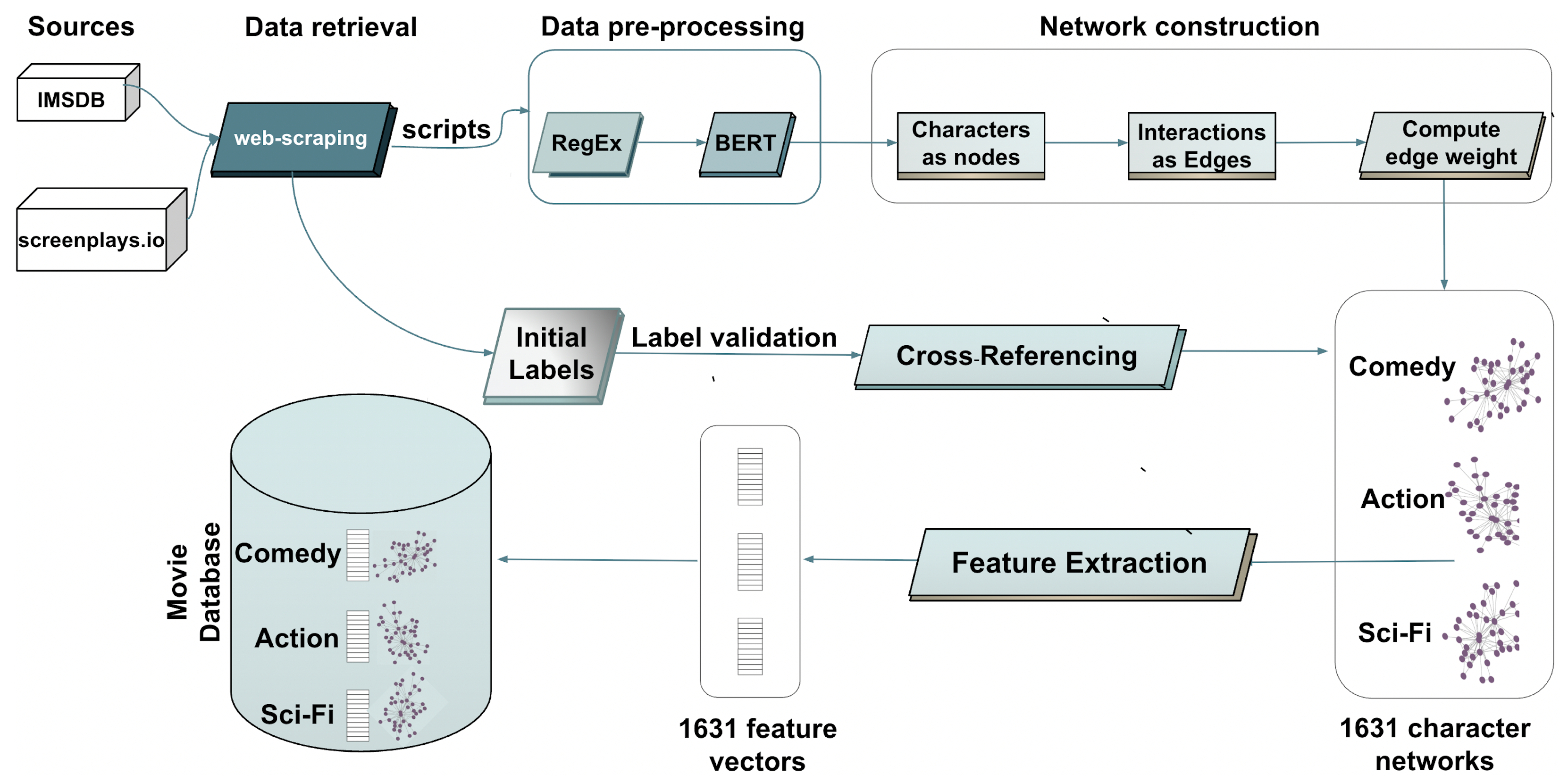
To address these limitations, we propose a method for processing a large number of movie scripts in minutes. In this section, we detail the procedures used to construct a character network from a movie script, following a multi-stage pipeline, moving from data retrieval to the topological representation. The overall process of construction is illustrated in Figure 2.

3.1.1. Data Retrieval and Pre-Processing

The initial stage of our pipeline focuses on automated document harvesting and text cleaning:

• Data Retrieval: We built custom web-scraping frameworks in Python 3.12.13, employing the BeautifulSoup4 library [32], to automate script retrieval.
• Character Entity Identification: Regular Expressions (RegEx) [33] were used to match uppercase strings to isolate potential character names.
• Entity Cleansing via RegEx: A filtering process is applied to minimize false positives from raw uppercase strings:

  –

  Metadata removing: Systematically removes parenthetical script modifiers often appended to names (e.g., VOICE OVER, CONT’D).

  –

  Technical Indicator Exclusion: Filters out false-positive production commands written in capital letters, explicitly excluding terms such as FADE IN, FADE OUT, FADE TO, INT., and CUT TO.

3.1.2. Entity Refinement via Transformer Model

Due to inconsistencies in script formatting, Regular Expressions may misidentify dialogue lines written in capital letters or scene headings that do not begin with technical indicators as character names. Despite applying Regular Expressions to maximize cleaning in the previous phase, a small proportion of errors persist, with some lines in capital letters incorrectly extracted as character names.

To address this, we implement a filtering layer using the BERT [34] (Bidirectional Encoder Representations from Transformers). This model is fine-tuned specifically for recognizing character names. For this purpose, we created a dataset that contains 18,349 instances. These instances include a mixture of character names, relevant keywords, and location names. The dataset was compiled from two sources: elements extracted directly from scripts and additional samples generated using AI techniques. After fine-tuning BERT on this comprehensive dataset, we applied the model to a list that initially contained errors related to character identification.

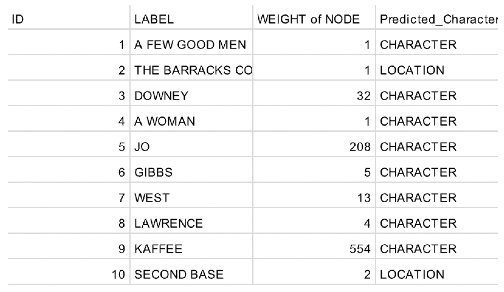
The trained BERT model was able to effectively differentiate between character names, dialogues, and location mentions, as illustrated in Figure 3. Following this classification, entries that were not valid character names were systematically removed. This process allowed us to retain only accurate character names for further use.

3.1.3. Character Network Topology and Edge Weighting

The character network $\mathcal{G}$ is conceptualized as an undirected graph an, where:

• The nodes $u\in \mathcal{U}$ represent the unique characters identified in the script.
• Edges $e_{u_1{u}_2}\in \mathcal{E}$ are established between characters in communication within the same scene.
• The edge weight is determined by the total frequency of interactions between a pair of characters throughout the entire movie, expressing the strength of the connection. The edge weight ${\omega }_{u_1{u}_2}$ between the character $u_1$ and $u_2$ is defined as the total number of interactions occurring across all n scenes in the movie. This is formally expressed as:

  $${\omega }_{u_1{u}_2}={\displaystyle \sum _{s=1}^n}{c}_{u_1{u}_2,s}$$

  (11)

  where $c_{u_1{u}_2,s}$ is a binary or frequency indicator representing the interaction between character i and character j within scene s.

3.2. Feature Vector Extraction

In [18], we introduced a methodology for classifying movie genres that relies on network properties and machine learning classifiers. For a character network $\mathcal{G}$, we systematically extract network features via Algorithm 1, then combine them in the output feature vector x.

The details of how the feature vector is built and the definitions of the network properties can be found in [18] and in Appendix A.

Algorithm 1 Feature Vector Extraction

input: $\mathcal{G}$ output: feature vector x 1: $\mathcal{D}\leftarrow mean(deg\left(u_1\right),deg\left(u_2\right),\dots ,deg\left(u_{\left|\mathcal{V}\right|}\right))$                                                                  // Node degree 2: $CC\leftarrow mean(CC\left(u_1\right),CC\left(u_2\right),\dots ,CC\left(u_{\left|\mathcal{V}\right|}\right))$                                                  // Clustering Coefficient 3: $BC\leftarrow mean(BC\left(u_1\right),BC\left(u_2\right),\dots ,BC\left(u_{\left|\mathcal{V}\right|}\right))$                                                // Betweenness Centrality 4: $Dens\leftarrow Dens\left(\mathcal{G}\right)$                                                                                                                     // Density 5: $C\leftarrow mean(C\left(u_1\right),C\left(u_2\right),\dots ,C\left(u_{\left|\mathcal{V}\right|}\right))$                                                                                         // Core 6: $T\leftarrow mean(T\left(u_1\right),T\left(u_2\right),\dots ,T\left(u_{\left|\mathcal{V}\right|}\right))$                                                                       // Triangle Count 7: $ecc\leftarrow mean(ecc\left(u_1\right),ecc\left(u_2\right),\dots ,ecc\left(u_{\left|\mathcal{V}\right|}\right))$                                                                     // Eccentricity 8: $netmf\leftarrow mean\left(NetMF\right(\mathcal{G}\left)\right)$                                                               // Network Matrix Factorization 9: $portrait\leftarrow mean(Singular\_Values(\mathcal{B}\left)\right)$       // Singular Value Decomposition of Network Portraits 10: ${\lambda }_{\mathbf{A}}\leftarrow mean\left(eigenvalues\left(\mathbf{A}\right)\right)$                                                                           // Adjacency Spectrum 11: ${\lambda }_{\tilde{\mathbf{L}}}\leftarrow mean\left(eigenvalues\left(\tilde{\mathbf{L}}\right)\right)$                                                      // Normalized Laplacian Spectrum 12: ${\lambda }_{\mathbf{L}}\leftarrow mean\left(eigenvalues\left(\mathbf{L}\right)\right)$                                                                             // Laplacian Spectrum 13: $netLSD\leftarrow mean\left(netLSD\right(\mathcal{G}\left)\right)$                                           // Network Laplacian Spectra Descriptor 14: $x\leftarrow [\mathcal{D},CC,BC,Dens,C,T,ecc,netmf,portrait,{\lambda }_{\mathbf{A}},{\lambda }_{\tilde{\mathbf{L}}},{\lambda }_{\mathbf{L}},netLSD]$

3.3. Intra-Cluster Weighted Movie Network (ICWMN) Construction

An Intra-Cluster Weighted Movie Network (ICWMN) is defined as a graph ${\mathcal{G}}_{IC}=(\mathcal{V},{\mathcal{E}}_{IC},\mathcal{W})$, where each node represents a movie network (Section 3.3.1) and is associated with a feature vector (Section Movie Node Feature Extraction and Selection). Edges are established between movies based on node similarity, with edge weights derived from this similarity.

3.3.1. Movie Nodes, $\mathcal{V}$

In the Intra-Cluster Weighted Movie Network (ICWMN), each node $v_i\in \mathcal{V}$ corresponds to a movie from the dataset. A node is not just an identifier but a representation of its corresponding character network ${\mathcal{G}}_i$, as detailed in Section 3.1. This construction captures the internal structural of the movie’s narrative. Consequently, the node $v_i$ functions as a composite entity whose features $x_i$ and relationships are entirely derived from the topological properties of its associated character network ${\mathcal{G}}_i$ (See Section 3.2).

3.3.2. Clustering

The key limitation of FCWMN arises when scaling to large networks with millions of edges. This is because GNNs perform message passing between every pair of connected nodes. Indeed, in a fully connected network with a large number of nodes, this results in message passing through millions of edges, leading to significant computational cost and noisy learning. To address this, we partition the movie network into clusters, minimizing unnecessary edges and focusing on learning relevant structural patterns.

Li et al. [35] developed Cluster-GCN, an algorithm for learning large-scale networks. Their empirical study demonstrated that, on such graphs, clustering is highly effective in training GCNs. For a graph with 2 million nodes and 61 million edges, Cluster-GCN achieved a training time per epoch of only 2.02 s and required only 2.3 GB of memory. In addition, the authors found that the clustering partition method is significantly more efficient than random partitioning.

Clustering refers to the computational process of dividing a dataset into groups or categories [36]. Although researchers have not established a standard definition for the term Clustering, most frameworks characterize a cluster based on two primary criteria: internal similarity and external divergence. This limitation has been demonstrated by an impossibility theorem [37], which shows that no clustering algorithm can be effectively applied to all types of datasets or problem scenarios.

A plethora of clustering techniques exist, such as those based on distance and similarity measures [38], hierarchical methods [39], graph theory-based approaches [40], and fuzzy clustering [41], among others. In this study, we chose to use clustering based on distance measures. This method is based on distance measures such as cosine similarity and Person correlation. In this study, we use five distance measures: NetLSD [23], D-measure [27], Portrait Divergence [22], Laplacian, and NetMF [26].

3.3.3. Edges, ${\mathcal{E}}_{IC}$

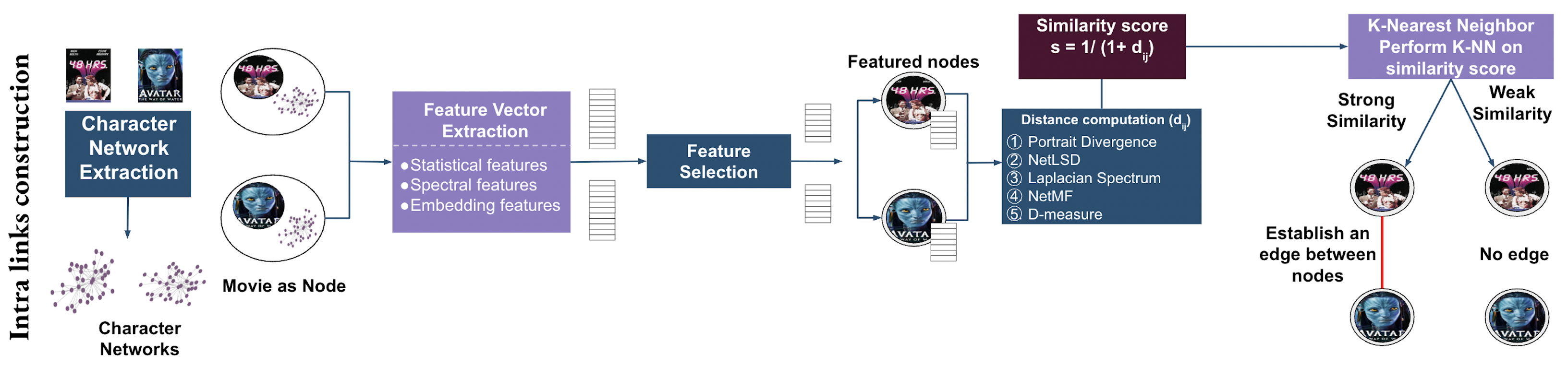
The Intra-cluster Weighted Movie Network (ICWMN) is defined by a set of edges ${\mathcal{E}}_{IC}$, which comprises intra-cluster connections. An intra-cluster edge $(v_1,v_2)\in {\mathcal{E}}_{IC}$ connects a pair of movie nodes if they reveal a high similarity between their corresponding character networks. Based on a similarity measure, the K-Nearest Neighbors (K-NN) algorithm is applied within each category to identify the k most structurally similar neighbors for each movie node. By connecting only the most similar nodes, this approach ensures that message passing (Section 2.2.1) is restricted to the most relevant movie pairs.

The fundamental principle of the nearest neighbor technique centers on assigning a label to an unclassified instance by identifying the closest pre-labeled neighboring data point [42]. A plethora of nearest neighbor extensions has been developed. K-Nearest Neighbor [43], assigns a category to an instance based on the majority vote of its k most proximal neighbors. Weighted k nearest neighbor [44], assigns weights to training data points based on their distance from a sample instance. The Model-Based K-NN  [45], functions by first choosing appropriate metrics to generate a comprehensive similarity matrix from the training data. Within each cluster, K-NN identifies the k neighbor closest to it. Simultaneously, the algorithm finds data points that belong to the most distant clusters.

In this paper, we employ three distance metrics $d_{ij}$ to implement the K-NN algorithm to construct relationships between movie nodes in our dataset, each capturing different aspects of the networks’ topology: (1) NetLSD [23], (2) Laplacian Spectrum, and (3) Network Portrait Divergence [22].

The similarity, $s_{ij}$ quantifies the structural similarity between the character networks, ${\mathcal{G}}_i$ and ${\mathcal{G}}_j$, of the corresponding movie nodes, following the methodology proposed in [24].

We define the similarity score, $s_{ij}$, as a value derived from the calculated distance $d_{ij}\in [0, 1]$ using Equation (12).

$$s_{ij}={\displaystyle \frac{1}{1+d_{ij}}}$$

(12)

The construction of the Intra-Cluster Weighted Movie Network is detailed in Algorithm 2 and Figure 4.

Algorithm 2 Intra-Cluster Weighted Movie Network Construction

input: $\mathcal{V}=\{v_1,\dots ,v_n\}$ : Movie nodes. $\mathcal{L}:\mathcal{V}\to \mathcal{C}$         : Mapping function, where $\mathcal{C}$ is the set of categories. $\mathcal{D}\in {\mathbb{R}}^{n\times n}$         : Distance matrix. $k\in {\mathbb{Z}}^{+}$              : Number of neighbors. output: $\mathcal{G}=(\mathcal{V},{\mathcal{E}}_{IC})$: Intra-cluster graph. 1: Distance: Compute the distance matrix $\mathcal{D}$ using a distance measure, such that: $$\mathcal{D}={\left(d_{i,j}\right)}_{v_i,v_j\in \mathcal{V}}$$ 2: For each node $v_i\in \mathcal{V}$, identify the K-Nearest Neighbor ${\mathcal{N}}_i\subset \mathcal{V}\setminus \left\{v_i\right\}$ such that: $$|{\mathcal{N}}_i|=k,\forall v_j\in {\mathcal{N}}_i,\forall v_l\notin {\mathcal{N}}_i\cup \left\{v_i\right\},d_{k_{i,j}}\le d_{k_{i,l}}$$ 3: $\forall v_i,v_j\in \mathcal{N}$, an Intra-cluster edge is established between $v_i$ and $v_j$ if $s_{ij}\simeq 1$, such that: $$s_{i,j}={\displaystyle \frac{1}{1+d_{i,j}}}$$ 4: If an edge exists between two nodes, the distance $d^{\prime }$ between them is computed. This distance value is then assigned as the edge weight, such that: $$w_{v_i,v_j}=d_{v_i,v_j}^{\prime }$$

3.3.4. Weighting, $\mathcal{W}$

The weight ${\omega }_{ij}$ assigned to an edge between two movie nodes $v_i$ and $v_j$ reflects the distance between their corresponding character networks. This distance is computed using one of three distance measures defined in Section 2.1: the NetLSD, the Laplacian spectrum, and the Network Portrait Divergence. The implementation of these measures follows Algorithms 1–5 as described in [24], which have been consistently applied to the movie network datasets within the present study. For each pair of adjacent nodes $v_i$ and $v_j$, we compute the distance using one of these measures and attribute the resulting value as the edge weight.

3.3.5. Node Classification

Movie Node Feature Extraction and Selection

Each movie node $v_i$ in the ICWMN is associated with a high-dimensional feature vector $x_i$, which encapsulates the structural properties of its corresponding character network ${\mathcal{G}}_i$, as detailed in Algorithm 1. The result is a feature matrix, $\mathcal{X}=\{x_1,x_2,\dots ,x_N\}$, where N is the total number of movies.

Feature selection [46,47,48,49] identifies a subset of relevant features that best represent the data, reducing redundancy and noise to improve classification performance. Removing irrelevant, noisy, and highly correlated features is crucial for improving both prediction accuracy and computational efficiency in deep learning tasks, thus preventing the degradation of GNN performance and reducing the risk of overfitting.

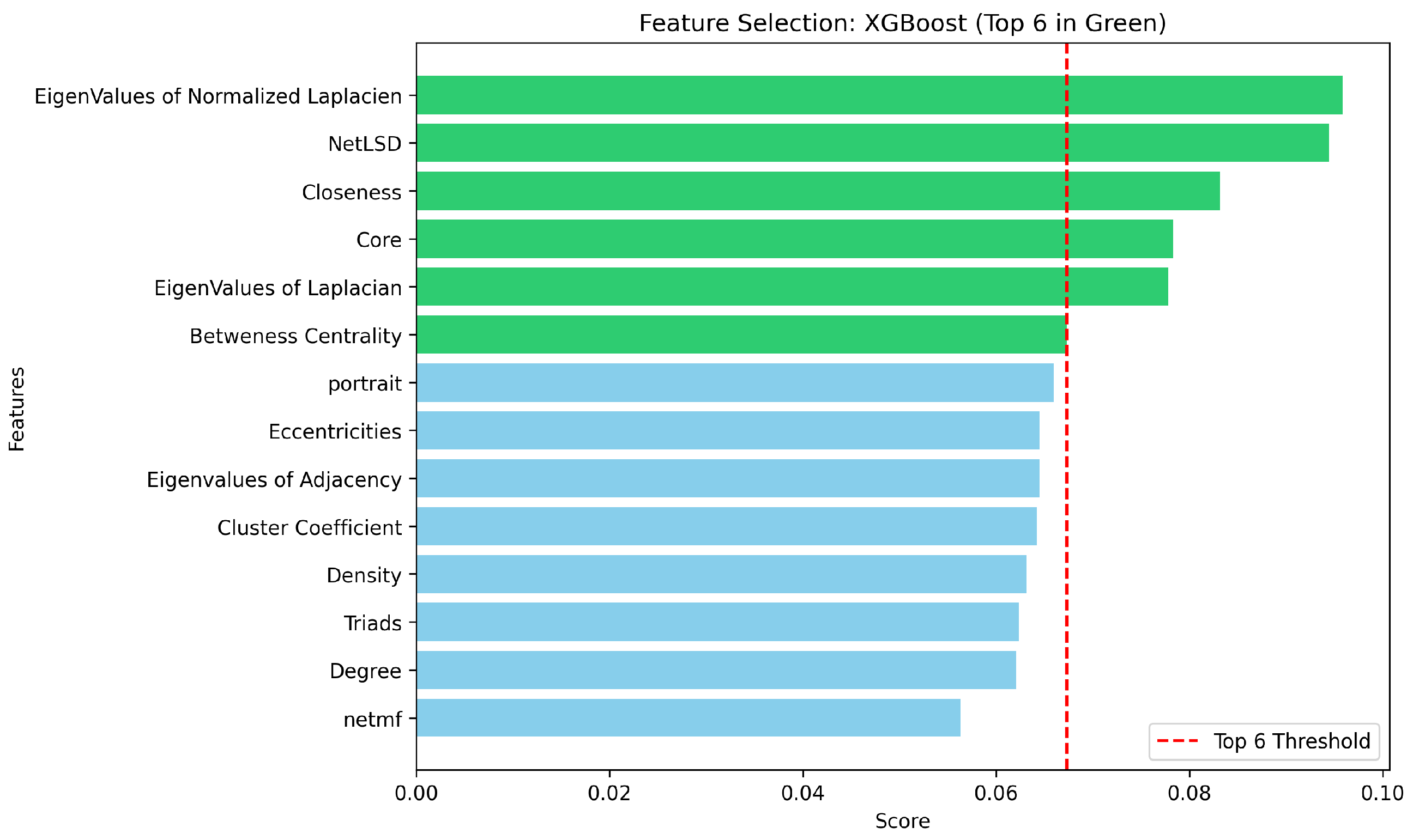
In the literature, there are three types of feature selection methods: Filter, Wrapper, and Embedding. In this study, we randomly selected one algorithm from each category—XGBoost [50], SelectkBest [51], and Random Forest [52] to identify the most appropriate network properties of the initial feature vector $\mathcal{X}$. This optimized matrix serves as the initial input for the GNN aggregation layers. In this paper, we present our analysis on the structural configurations derived from XGBoost. This choice is justified by the fact that all three paradigms result in near identical classification metrics. The feature set selected by XGBoost is illustrated in Figure 5.

Graph Neural Networks (GNN)

The final stage consists of applying GNN models to ICWMN. We selected GAT, GCN, and GraphSAGE because of their ability to incorporate edge weights. The input for any of GNN models employed in this study consists of three primary components: the feature matrix $\mathcal{X}$, the adjacency matrix $\mathcal{A}$, and the edge weight matrix $\mathcal{W}$.

The first step consists of normalizing the feature matrix $\mathcal{X}$ using the MinMaxScaler. This linear transformation scales the data into a range of [0, 1], preventing features with larger values from dominating those with smaller values according to the following formula:

$$x_{scaled}={\displaystyle \frac{x-x_{min}}{x_{max}-x_{min}}}$$

In the second step, the normalized feature matrix $X_{scaled}$, the adjacency matrix $\mathcal{A}$, and the edge weight matrix $\mathcal{W}$ are fed simultaneously into the first convolutional layer. One training cycle is composed of the forward and backward passes. On the forward pass, a convolution layer process $X_{scaled}$, $\mathcal{A}$, and $\mathcal{W}$ through the model to compute predictions. At this stage, each node $v_i$ updates its own feature representation $x_i$ by aggregating feature vectors from its connected neighbors $v_j$ using the mean aggregation operator ${\mathrm{mean}}_{j\in \mathcal{N}\left(v_i\right)}\psi (x_i^{\left(l\right)},x_j^{\left(l\right)})$. According to Equation (5), the updated feature vector $x_{v_i}^{\prime }$ for a node $v_i$ is computed as follows:

$$x_{v_i}^{\prime }=\varphi \left(x_{v_i},mea{n}_{j\in \mathcal{N}\left(v_{v_i}\right)}\psi \left(x_{v_i},x_{v_j}\right)\right)$$

(13)

The mechanism for combining feature vectors varies according to the convolutional architecture employed—GCN, GAT, or GraphSAGE—as follows.

GCN Convolution performs multiplication between the updated feature vector $X^{\prime }=\{x_1^{\prime },x_2^{\prime },...,x_N^{\prime }\}$, the weight matrix $\mathcal{W}$, and the normalized adjacency matrix ${\Delta }^{-1/2}\mathcal{A}{\Delta }^{-1/2}{\mathcal{X}}^{(l-1)}$ following Equation (14):

$$\mathcal{H}=ELU\left({\Delta }^{-1/2}\mathcal{A}{\Delta }^{-1/2}{\mathcal{X}}^{\prime }\mathcal{W}\right)$$

(14)

where the Exponential Linear Unit ($ELU$) [53] is used as the activation function to maintain a small gradient for negative inputs, which helps the network maintain a mean activation closer to zero and keep a stable gradient. The output is an embedding matrix $\mathcal{H}$, which serves as the input for the next convolutional layer.

GAT Convolution employs the self-attention mechanism to learn the importance of each neighboring node during the aggregation process. According to Equation (6), the attention coefficient ${\alpha }_{v_i{v}_j}$, which represents the importance of node $v_j$ to node $v_i$, is computed as follows:

$${\alpha }_{v_i{v}_j}=softmax\left(a_{v_i{v}_j}\right)={\displaystyle \frac{exp\left(a_{v_i{v}_j}\right)}{{\sum }_{k\in {\mathcal{N}}_i}exp\left(a_{v_i{v}_k}\right)}}$$

(15)

where $a_{v_i{v}_j}\in \mathcal{A}$, an element of the adjacency matrix.

The edge weight matrix $\mathcal{W}$ is used to guide these attention coefficients during the feature combination process. In this architecture, we employ multi-head attention with two heads ($att=2$). The output embedding matrix $\mathbf{H}$ is computed by concatenating (‖) the results from each head:

$${\mathcal{H}=\Vert }_{att=1}^{\mathbf{2}}ELU\left(\sum _{j\in {\mathcal{N}}_i}{\alpha }_{v_i{v}_j}^{att}{\mathcal{W}}^{att}{\mathcal{X}}^{\prime }\right)$$

(16)

GraphSAGE Convolution concatenates the updated feature matrix ${\mathcal{X}}^{\prime }$ computed during the aggregation process with the feature matrix before aggregation as shown in Equation (17). Then multiply it with the weight matrix $\mathcal{W}$ as follows.

$$\mathcal{H}=ELU\left(\mathcal{W}·\mathrm{CONCAT}\left(\mathcal{X},{\mathcal{X}}^{\prime }\right)\right)$$

(17)

All models are composed of five convolutional layers, where the first four layers are followed by an ELU activation function and a dropout layer. The output embedding matrix $\mathcal{H}$ of the fifth convolutional layer is passed through a softmax function to produce the final genre classification probabilities.

The dropout layer randomly deactivates a fraction of neurons during training. This technique prevents the network from becoming overly dependent on specific combinations of features, thereby reducing overfitting and improving generalization.

We have used Adam optimizer [54], one of the most popular gradient descent optimization algorithms.

On the backward pass, the network learns from its errors to improve classification accuracy thanks to the gradient of the loss ${\displaystyle \frac{\partial \mathrm{Loss}}{\partial \mathcal{W}}}$. So that the updated weight matrix becomes:

$${\mathcal{W}}^{\prime }=\mathcal{W}·\eta ·{\displaystyle \frac{\partial \mathrm{Loss}}{\partial \mathcal{W}}}$$

(18)

with ($\eta$) is a learning rate and ${\mathcal{W}}^{\prime }$ is the updated weighted matrix after each training cycle.

To evaluate our model, we opted for k-fold cross-validation [55] to ensure that in each cycle, a subset is reserved to assess the model’s performance while the remaining subsets are used for training.

4. Experimental Evaluation

In this section, we present the experimental results obtained by applying our proposed framework to two datasets: the 1631 movie networks we created for this study (Section 3.1) and the Moviegalaxies [56] dataset consisting of 773 movie networks. We applied the selection algorithms, XGBoost, to the datasets, identifying the six most significant features. The analysis evaluates the classification performance on weighted movie networks, and is detailed in Section 4.3.3. Furthermore, a comparative analysis between our findings and existing state-of-the-art methods is presented.

4.1. Database Construction

For this study, we constructed a novel database comprising 1631 movies, with corresponding feature vectors and target labels. The database construction process is illustrated in Figure 2, encompassing several key stages. Initially, movie scripts were harvested from the Internet Movie Script Database (IMSDB) and screenplays.io, using data retrieval through web scraping as shown in Section 3.1.1. This was followed by data processing using Regex and BERT (Section 3.1.2) and edge weight calculation (Section 3.1.3).

By applying this extraction pipeline, we constructed a comprehensive dataset comprising 1631 unique character networks. While the original movie scripts were pre-labeled with genre classifications upon retrieval from their respective source repositories, we implemented a rigorous validation phase to ensure label consistency. Each movie was individually cross-referenced against metadata retrieved via Google Search to verify its genre assignment and maintain the integrity of the dataset for subsequent analysis.

The Algorithm 1 is automatically applied to each of the 1631 character networks, producing a feature vector associated with each network. The resulting output is a database comprising 1631 character networks, where each network is associated with a high-dimensional feature vector and its corresponding genre label.

4.2. Experiment Setup

In this section, we present the hyperparameters used for configuration of the GAT, GCN, and GraphSAGE models during the experimental phase. The dataset was randomly split into 80% for training, 10% for validation, and 10% for testing.

A 5-fold cross-validation was selected to provide a reliable evaluation of the model’s performance without making the calculations too complex or slow.

We performed an ablation study to find the best depth for our models, testing different configurations starting from three layers. We found that a five-layer architecture worked best; it was deep enough to capture complex relationships within the movie network while avoiding the common issues of over-fitting and over-smoothing. For each model, we set the first four convolutional layers to a 64-unit hidden dimension, while the output of the final layer was matched to the number of target classes. In the GAT model, we used two attention heads, which was subsequently reduced to a single attention head in the final output layer.

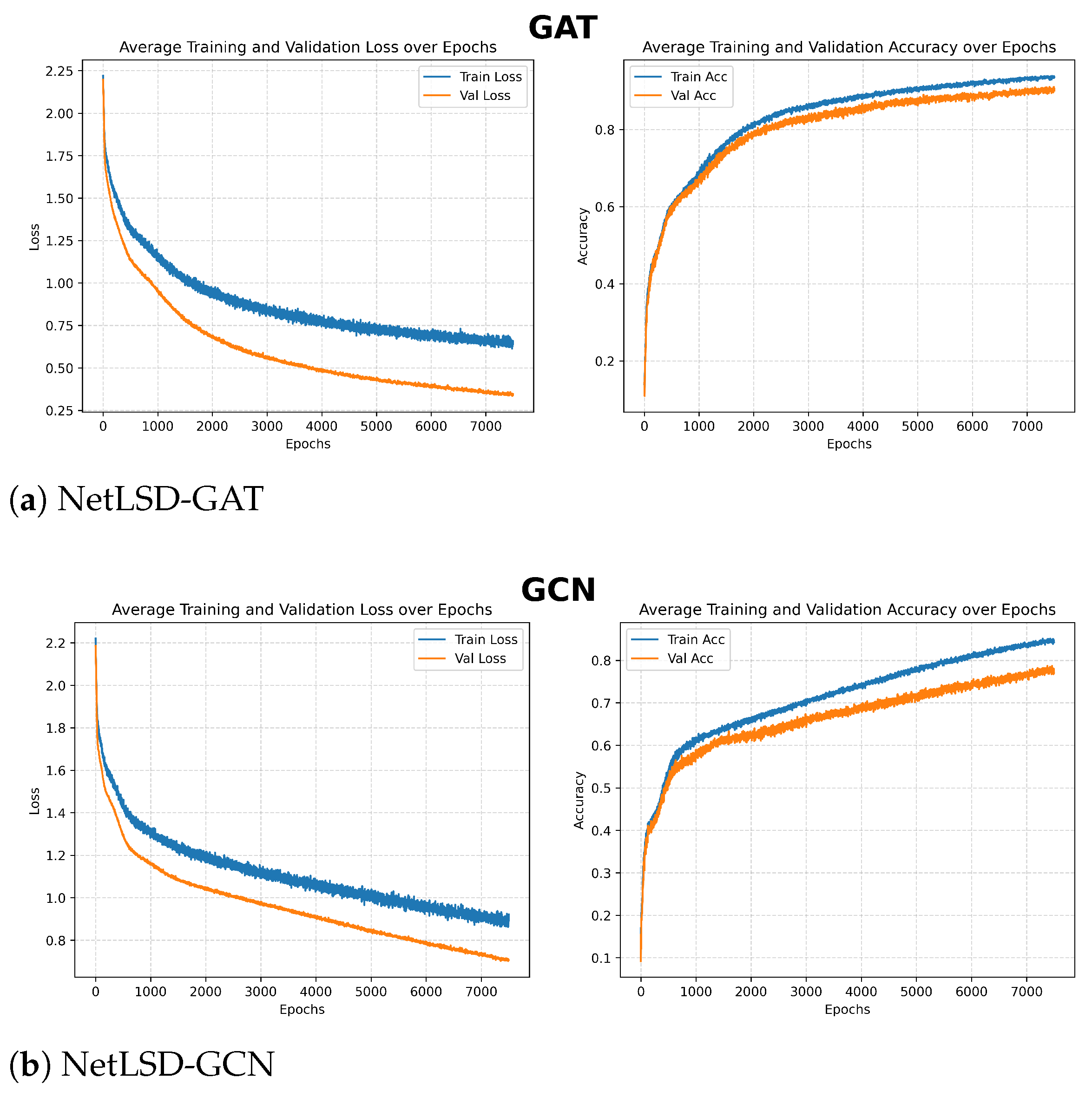
All models were trained for 7500 epochs using the Adam optimizer [54]. A learning rate of $1\times {10}^{-3}$ was selected. To further protect against overfitting and improve the generalization of the model, we applied a weight decay of $5\times {10}^{-4}$. This regularization penalizes excessively large weights, forcing the network to focus on essential patterns rather than memorizing noise, which ultimately improves its ability to generalize to new data [57] (Figure 6).

Table 1. Hyperparameter settings for GAT, GCN, and GraphSAGE models.

Hyperparameters	GAT	GCN	GraphSAGE
Number of Hidden Layers	64	64	64
Number of Attention Heads	2	-	-
Activation function	ELU	ELU	ELU
Dropout	20%	20%	20%
Optimizer	Adam	Adam	Adam
Weight Decay	$5\times {10}^{-4}$	$5\times {10}^{-4}$	$5\times {10}^{-4}$
Learning Rate	$1\times {10}^{-3}$	$1\times {10}^{-3}$	$1\times {10}^{-3}$
Total Training Steps	7500	7500	7500

summarizes these hyperparameter settings for the GAT, GCN, and GraphSAGE models.

4.3. Experimental Results

4.3.1. Data Processing and Character Network Scalability

To evaluate the scalability of our framework, execution runtime and memory usage were tracked throughout the entire pipeline. As shown in

Table 2. Execution time and memory usage for BERT training, label prediction, and interaction construction steps using a GPU.

	Time (s)	Memory Usage (MB)
Train BERT on 18,349 instances	717.51	835.56
Predict labels for 1631 movies (BERT)	108.14	0
1631 interaction construction	147.70	0

, the automated pipeline completely eliminates the heavy manual overhead required by MovieNet [31], which required approximately 15 days of manual processing for only one script to match characters with subtitles.

Upfront offline training of the BERT model using 18,349 instances represents the primary computational overhead, requiring 717.51 s (≈12 min) and 835.56 MB of peak memory. Crucially, as a one-time operation, this does not restrict deployment scalability. High-throughput inference across all 1631 unstructured movie scripts is completed in just 108.14 s, followed by character interaction construction within 147.70 s.

Consequently, the end-to-end network synthesis for the entire dataset requires a post-training runtime of only 255.84 s (≈4.2 min) on a GPU with negligible active memory usage (≈0 MB). This compresses the processing latency from 15 days down to a fraction of a second per movie, demonstrating a highly scalable solution for large-scale Graph Neural Network (GNN) applications.

4.3.2. Sensitivity to K

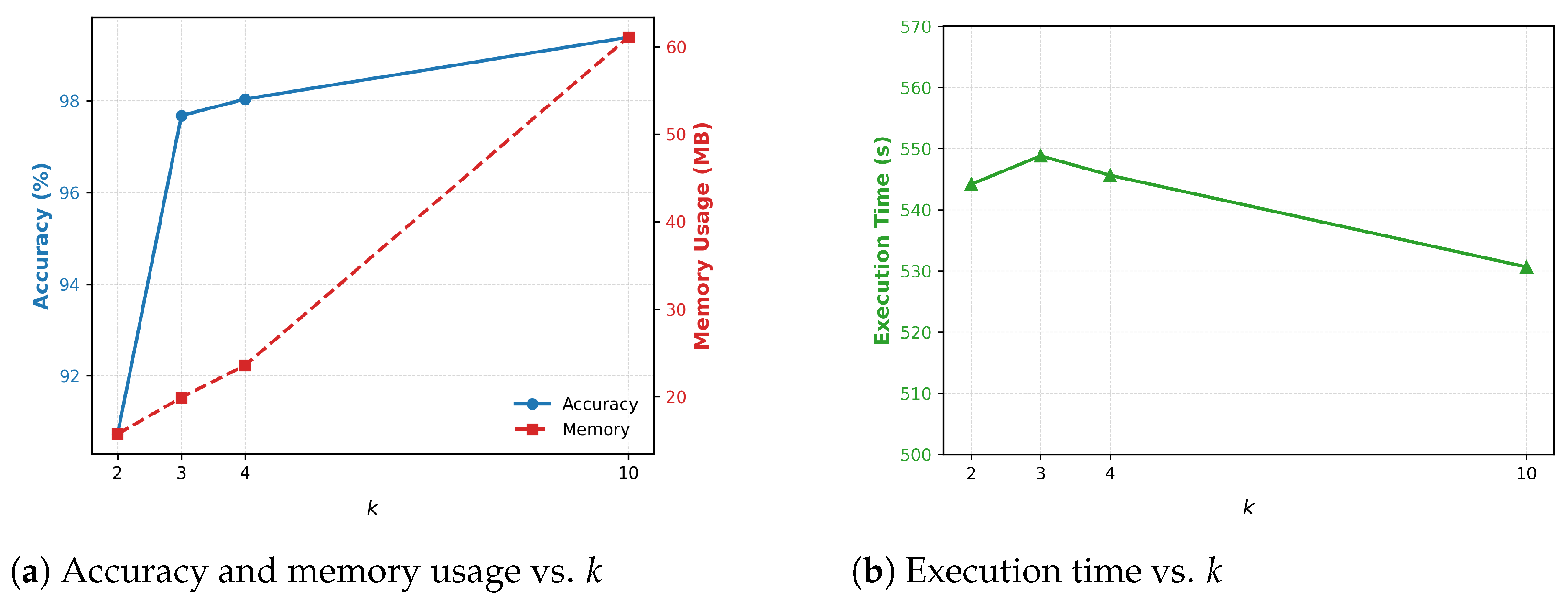
As illustrated in Figure 7, we conducted a sensitivity analysis on the NetLSD-based network based on $k\in \{2,3,4,10\}$ to evaluate the impact of k on classification accuracy, execution time, and memory usage. Increasing k from 2 to 3 results in a significant accuracy improvement of $6.95\%$, reaching $97.68\%$. Beyond this inflection point, the accuracy improvements enter a saturation phase, increasing marginally by only $1.71\%$ from $k=3$ to $k=10$, while the memory usage increases significantly from $19.90$ MB to $61.07$ MB. Since the execution time remains relatively stable across all configurations, $k=3$ is selected as the optimal hyperparameter, offering the most efficient balance between topological representation and hardware memory allocation.

4.3.3. Performance Metrics on the 1631 and 773 Movie Datasets

The comparative classification results for the two movie network datasets are summarized in

Table 3. Comparative performance of the 1631 movie network dataset across various edge weight measures using XGBoost feature selection. Values represent test accuracy(%). Values in bold represent the highest classification accuracy achieved for each network configuration.

		K-NN Distance
		Portrait Div. Network			NetLSD Network			Laplacian Network
		GAT	GCN	SAGE	GAT	GCN	SAGE	GAT	GCN	SAGE
Edge Weight	Laplacian	80.73	75.00	76.82	90.04	77.68	80.85	95.00	82.56	89.02
	NetLSD	79.63	74.02	76.82	89.51	76.95	80.48	93.90	81.95	88.53
	Portrait Div.	80.12	75.36	75.24	91.71	78.29	82.32	94.51	81.95	88.90

(1631-movie dataset) and

Table 4. Comparative performance of the 773 movie network dataset across various edge weight measures using XGBoost feature selection. Values represent test accuracy(%). Values in bold represent the highest classification accuracy achieved for each network configuration.

		K-NN Distance
		Portrait Div. Network			NetLSD Network			Laplacian Network
		GAT	GCN	SAGE	GAT	GCN	SAGE	GAT	GCN	SAGE
Edge Weight	Laplacian	94.86	74.59	90.27	88.38	64.05	75.68	97.30	86.76	95.14
	NetLSD	97.30	74.32	91.08	85.41	70.27	73.51	97.30	75.68	96.22
	Portrait Div.	94.59	72.97	88.92	83.51	64.59	71.62	97.30	81.62	95.68

(773-movie dataset). Both tables evaluate the performance of three GNN architectures—GAT, GCN, and GraphSAGE—across various edge weight configurations and K-NN distance networks.

Overall, the empirical results demonstrate exceptional classification performance, with several topological configurations producing high-tier accuracies, peaking at $95.00\%$ for GAT in the 1631 dataset in Table 3 and $97.30\%$ for GAT in the 773 dataset in Table 4.

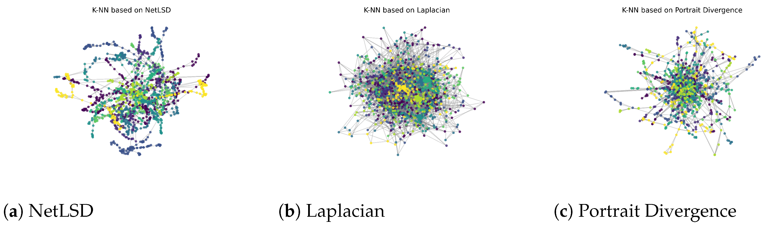
To visually inspect the structural separability of our proposed framework, we provide a directed network visualization of the ICWMN under different distance configurations in Figure 8. A clear topological contrast can be observed between the metrics:

• The NetLSD network (Figure 8a) and the Portrait Divergence network (Figure 8c) generate highly filamentary structures with long, distributed branches. This indicates that these metrics focus extensively on specific multi-scale heat-kernel traces or localized degree distribution patterns.
• In contrast, the Laplacian Network (Figure 8b) forces a highly cohesive, well-bound, and dense structural grouping. The global spectral geometry encoded by the Laplacian matrix effectively forces graphs belonging to structurally homogeneous genre categories into distinct and highly dense neighborhoods within the K-NN topology.

This visual behavior directly explains why the Laplacian configuration dominates the performance tables across all GNN models; it structurally optimizes the neighborhood information before the graph convolutions even take place.

A deeper analysis of the architectural behaviors suggests a scale-dependent performance variation between the two datasets.

• GAT displays the highest degree of structural stability and dominance in both datasets. It consistently claims the absolute maximum peak across both datasets ($95.00\%$ in Table 3 and $97.30\%$ in Table 4). It maintains tightly bounded high-accuracy scores, rarely dropping below $80\%$, proving that attention mechanisms effectively weigh structural features regardless of the underlying dataset scale.
• GraphSAGE is identified as the second most effective architecture across both corpora. When deployed on the Laplacian Network representation, GraphSAGE consistently demonstrates strong performance, attaining a maximum accuracy of $89.02\%$ on the larger corpus (Table 3) and reaching up to $96.22\%$ on the smaller 773 network corpus (Table 4) when combined with NetLSD edge weights. These results underscore GraphSAGE’s efficiency in using neighborhood sampling techniques to capture robust structural relationships in larger graph distributions.
• GCN, although competitive under certain global configurations, demonstrates inferior performance compared to GAT and GCN models when localized topologies are subject to structural constraints. This is particularly evident within the NetLSD distance framework applied to the smaller corpus (Table 4), where the accuracy drops significantly to $64.05\%$. However, standard graph convolutions converge more effectively when supported by the structural properties of the Laplacian Network, resulting in GCN achieving $82.56\%$ and $86.76\%$ in Table 3 and Table 4, respectively.

All in all, the consistency of the cross-architecture observed in both tables serves as a strong statistical validation for our feature representation methodology. In both Table 3 and Table 4, the Laplacian Network reveals the highest classification accuracy, regardless of whether GAT, GCN, or GraphSAGE is used. This multi-model alignment establishes that the global spectral feature captured by the Laplacian matrix provides inherently superior topological expressivity to distinguish complex structural properties within movie genres.

4.3.4. Benchmark Comparison Against the State-of-the-Art

Table 5. The comparison of ICWMN with the state of the arts. All methods were evaluated using the 1631 movie network database.

Methods	Accuracy (%)	Precision (%)	Recall (%)	F1-Score (%)
Mizvol et al. [20]	16	14	17	14
Lafhel et al. [18]	67	66.66	66.66	65.95
FCWMN using GCN [21]	65.05	71.38	65.53	64.17
ICWMN using GCN	82.56	83.68	84.21	83.60
ICWMN using GraphSAGE	89.02	90.27	90.35	89.43
ICWMN using GAT	95.00	95.04	95.89	95.29

and

Table 6. The comparison of ICWMN with the state of the arts. All methods were evaluated using the 773 movie network database.

Methods	Accuracy (%)	Precision (%)	Recall (%)	F1-Score (%)
Mizvol et al. [20]	27	27	27	27
Lafhel et al. [18]	92	89	89	89
FCWMN using GCN [21]	87	93	88	88
ICWMN using GCN	86.76	86.74	85.70	85.03
ICWMN using GraphSAGE	96.22	96.11	98.00	96.63
ICWMN using GAT	97.30	96.42	98.57	97.20

provide a comprehensive benchmark of the proposed ICWMN framework against the existing literature and current state-of-the-art methods. The results reveal a significant performance progress across all evaluation metrics, including Accuracy, Precision, Recall, and F1-Score, confirming the structural prominence of the weighted spectral approach.

A crucial matter in this study is the evolution from the Fully Connected Weighted Movie Network (FCWMN) [21] to the current ICWMN. While the FCWMN used a weighted architecture where all nodes were interconnected, the ICWMN introduces a more refined topology. By moving away from fully connected nodes to clusters, we achieved a significant accuracy increase. For instance, in the 1631 dataset (Table 5), the FCWMN using GCN reached an accuracy of $65.05\%$, whereas the proposed ICWMN using GAT framework significantly improved this metric to $95.00\%$, with a corresponding F1-Score of $95.29\%$.

Compared to external benchmarks such as Mizvol et al. [20], which shows only 16% accuracy, the proposed ICWMN maintains adequate performance. This performance gap confirms that while our earlier weighted models (FCWMN) were a significant step in the right direction, the current approach—based on the Laplacian K-Nearest Neighbor topology and Laplacian edge weights—represents the definitive solution for high-precision movie genre classification.

This performance is consistently maintained across the smaller dataset comprising 773 movie networks, as detailed in Table 6. Within this corpus, state-of-the-art models proposed by Mizvol et al. and Lafhel et al. achieve classification accuracies of 27% and 92%, respectively, while the FCWMN, utilizing a Graph Convolutional Network, achieves an accuracy of 87%.

In contrast, the proposed ICWMN framework demonstrates superior performance. Specifically, the ICWMN employing a GCN attains a raw accuracy of $86.76\%$, which is highly comparable and nearly identical to the $87\%$ attained by the FCWMN, indicating only a negligible difference. Notably, both the GraphSAGE and GAT architectures of ICWMN substantially exceed the previous state-of-the-art results. The ICWMN employing GraphSAGE achieves an accuracy of $96.22\%$, while the highest value is obtained using the GAT configuration, reaching an accuracy of $97.3\%$. This consistency across various architectural configurations substantiates the structural expressiveness of the proposed ICWMN framework, demonstrating that reducing the number of edges effectively diminishes topological noise and consequently enhances the capability for movie genre classification.

5. Conclusions

The experimental results reveal several key findings regarding the performance and scalability of the proposed framework. Notably, the transition from the Fully Connected Weighted Movie Network (FCWMN) to the Intra-Cluster framework (ICWMN) substantially increased classification accuracy. For instance, on the 1631 dataset, the FCWMN using GCN achieved $65.05\%$, whereas the proposed ICWMN using the GAT architecture improved this metric to a peak of $95\%$.

Across both evaluation datasets, and regardless of whether GCN, GAT, or GraphSAGE architectures were employed, constructing the underlying network topology using the Laplacian Network distance consistently resulted in the highest classification accuracy.

A clear, scale-dependent variation in model performance was observed. GAT was identified as the top-performing architecture across both datasets, achieving a maximum accuracy of $95\%$ on the larger dataset, which comprised 1631 movie networks, and reaching a maximum of $97.30\%$ accuracy on the smaller dataset with 773 movie networks. GraphSAGE was the second most effective model, capturing robust structural relationships across both corpora, with a peak accuracy of $96.22\%$ on the 773 dataset. In contrast, the GCN stabilized at approximately $86.76\%$ when mapped via the Laplacian Network. However, its accuracy remains highly comparable to its predecessor.

Our pipeline to extract a character network from a script demonstrates exceptional scalability; following a one-time offline BERT training session of approximately 12 min, high-throughput inference across all 1631 unstructured movie scripts requires just 108.14 s, and interaction network construction completes in 147.70 s.

In future work, we will focus on expanding the ICWMN framework by integrating other GNN architectures, such as Graph Transformers and Edge Convolutions. In addition, we intend to evaluate other feature selectors beyond those currently employed to identify even more robust topological features for movie genre classification. Finally, we plan to implement the ICWMN framework in a keyword database.

References

1. Rasheed, Z.; Shah, M. Movie genre classification by exploiting audio-visual features of previews. In Proceedings of the 2002 International Conference on Pattern Recognition; IEEE: New York, NY, USA, 2002; Volume 2, pp. 1086–1089. [Google Scholar]
2. Zhou, H.; Hermans, T.; Karandikar, A.V.; Rehg, J.M. Movie genre classification via scene categorization. In Proceedings of the 18th ACM International Conference on Multimedia, Firenze, Italy, 25–29 October 2010; pp. 747–750. [Google Scholar]
3. Chu, W.T.; Guo, H.J. Movie genre classification based on poster images with deep neural networks. In Proceedings of the Workshop on Multimodal Understanding of Social, Affective and Subjective Attributes, Mountain View, CA, USA, 27 October 2017; pp. 39–45. [Google Scholar]
4. Simões, G.S.; Wehrmann, J.; Barros, R.C.; Ruiz, D.D. Movie genre classification with convolutional neural networks. In Proceedings of the 2016 International Joint Conference on Neural Networks (IJCNN); IEEE: New York, NY, USA, 2016; pp. 259–266. [Google Scholar]
5. Behrouzi, T.; Toosi, R.; Akhaee, M.A. Multimodal movie genre classification using recurrent neural network. Multimed. Tools Appl. 2023, 82, 5763–5784. [Google Scholar] [CrossRef]
6. Chakrabarti, S.; Dom, B.; Indyk, P. Enhanced hypertext categorization using hyperlinks. Acm Sigmod Rec. 1998, 27, 307–318. [Google Scholar] [CrossRef]
7. Zhur, X.; Ghahramani, Z. Learning from labeled and unlabeled data with label propagation. ProQuest Number Inf. All. Users 2002. [Google Scholar]
8. Perozzi, B.; Al-Rfou, R.; Skiena, S. Deepwalk: Online learning of social representations. In Proceedings of the 20th ACM SIGKDD International Conference on Knowledge Discovery and Data Mining, New York, NY, USA, 24–27 August 2014; pp. 701–710. [Google Scholar]
9. Grover, A.; Leskovec, J. node2vec: Scalable feature learning for networks. In Proceedings of the 22nd ACM SIGKDD International Conference on Knowledge Discovery and Data Mining, San Francisco, CA, USA, 13–17 August 2016; pp. 855–864. [Google Scholar]
10. Bruna, J.; Zaremba, W.; Szlam, A.; LeCun, Y. Spectral networks and locally connected networks on graphs. arXiv 2013, arXiv:1312.6203. [Google Scholar]
11. Kipf, T.N.; Welling, M. Semi-supervised classification with graph convolutional networks. arXiv 2016, arXiv:1609.02907. [Google Scholar]
12. Hamilton, W.; Ying, Z.; Leskovec, J. Inductive representation learning on large graphs. Adv. Neural Inf. Process. Syst. 2017, 30. [Google Scholar]
13. Veličković, P.; Cucurull, G.; Casanova, A.; Romero, A.; Lio, P.; Bengio, Y. Graph attention networks. arXiv 2017, arXiv:1710.10903. [Google Scholar]
14. Kagan, D.; Chesney, T.; Fire, M. Using data science to understand the film industry’s gender gap. Palgrave Commun. 2020, 6, 92. [Google Scholar] [CrossRef]
15. Fei, N.; Zhang, Y. Movie genre classification using TF-IDF and SVM. In Proceedings of the 2019 7th International Conference on Information Technology: IoT and Smart City, Shanghai, China, 20–23 December 2019; pp. 131–136. [Google Scholar]
16. Huang, Y.F.; Wang, S.H. Movie genre classification using svm with audio and video features. In Proceedings of the Active Media Technology: 8th International Conference, AMT 2012, Macau, China, 4–7 December 2012; Proceedings 8; Springer: Berlin/Heidelberg, Germany, 2012; pp. 1–10. [Google Scholar]
17. Sirattanajakarin, S.; Thusaranon, P. Movie genre in multi-label classification using semantic extraction from only movie poster. In Proceedings of the 7th International Conference on Computer and Communications Management, Bangkok, Thailand, 27–29 July 2019; pp. 23–27. [Google Scholar]
18. Lafhel, M.; El Hassouni, M.; Cherifi, H. Learning Character Network Features for Movie Genre Classification. In Proceedings of the 2024 IEEE Thirteenth International Conference on Image Processing Theory, Tools and Applications (IPTA); IEEE: New York, NY, USA, 2024; pp. 1–6. [Google Scholar]
19. Perri, V.; Qarkaxhija, L.; Zehe, A.; Hotho, A.; Scholtes, I. One Graph to Rule them All: Using NLP and Graph Neural Networks to analyse Tolkien’s Legendarium. arXiv 2022, arXiv:2210.07871. [Google Scholar]
20. Mizvol. Notebook Viewer. 2024. Available online: https://nbviewer.org/ (accessed on 6 June 2024).
21. Lafhel, M.; El Hassouni, M.; Cherifi, H. Movie Genre Classification with Graph Convolutional Networks on Fully Connected Weighted Movie Networks. In Proceedings of the France’s International Conference on Complex Systems; Springer: Cham, Switzerland, 2025; pp. 206–217. [Google Scholar]
22. Bagrow, J.P.; Bollt, E.M. An information-theoretic, all-scales approach to comparing networks. Appl. Netw. Sci. 2019, 4, 45. [Google Scholar] [CrossRef]
23. Tsitsulin, A.; Mottin, D.; Karras, P.; Bronstein, A.; Müller, E. Netlsd: Hearing the shape of a graph. In Proceedings of the 24th ACM SIGKDD International Conference on Knowledge Discovery & Data Mining, London, UK, 19–23 August 2018; pp. 2347–2356. [Google Scholar]
24. Lafhel, M.; Cherifi, H.; Renoust, B.; El Hassouni, M. Comparison of graph distance measures for movie similarity using a multilayer network model. Entropy 2024, 26, 149. [Google Scholar] [CrossRef]
25. Mourchid, Y.; Renoust, B.; Cherifi, H.; El Hassouni, M. Multilayer network model of movie script. In Proceedings of the Complex Networks and Their Applications VII: Volume 1 Proceedings The 7th International Conference on Complex Networks and Their Applications COMPLEX NETWORKS 2018; Springer: Cham, Switzerland, 2019; Volume 1, pp. 782–796. [Google Scholar]
26. Qiu, J.; Dong, Y.; Ma, H.; Li, J.; Wang, K.; Tang, J. Network embedding as matrix factorization: Unifying deepwalk and line and pte and node2vec. In Proceedings of the Eleventh ACM International Conference on Web Search and Data Mining, Marina Del Rey, CA, USA, 5–9 February 2018; pp. 459–467. [Google Scholar]
27. Schieber, T.A.; Carpi, L.; Díaz-Guilera, A.; Pardalos, P.M.; Masoller, C.; Ravetti, M.G. Quantification of network structural dissimilarities. Nat. Commun. 2017, 8, 13928. [Google Scholar] [CrossRef] [PubMed]
28. Bagrow, J.P.; Bollt, E.M.; Skufca, J.D.; Ben-Avraham, D. Portraits of complex networks. Europhys. Lett. 2008, 81, 68004. [Google Scholar] [CrossRef]
29. Gilmer, J.; Schoenholz, S.S.; Riley, P.F.; Vinyals, O.; Dahl, G.E. Neural message passing for quantum chemistry. In Proceedings of the International Conference on Machine Learning; PMLR: New York, NY, USA, 2017; pp. 1263–1272. [Google Scholar]
30. Krizhevsky, A.; Sutskever, I.; Hinton, G.E. Imagenet classification with deep convolutional neural networks. Commun. ACM 2017, 60, 84–90. [Google Scholar] [CrossRef]
31. Mourchid, Y.; Renoust, B.; Roupin, O.; Văn, L.; Cherifi, H.; Hassouni, M.E. Movienet: A movie multilayer network model using visual and textual semantic cues. Appl. Netw. Sci. 2019, 4, 121. [Google Scholar] [CrossRef]
32. Richardson, L. Beautiful Soup Documentation, version 4.11.2, Computer Software. April 2007. Available online: https://www.crummy.com/software/BeautifulSoup/ (accessed on 7 October 2025).
33. Kleene, S.C.; Shannon, C.E.; McCarthy, J. Representation of Events in Nerve Nets and Finite Automata; Princeton University Press: Princeton, NJ, USA, 1956; Volume 34. [Google Scholar]
34. Devlin, J.; Chang, M.W.; Lee, K.; Toutanova, K. Bert: Pre-training of deep bidirectional transformers for language understanding. In Proceedings of the 2019 Conference of the North American Chapter of the Association for Computational Linguistics: Human Language Technologies, Volume 1 (Long and Short Papers); Association for Computational Linguistics: Stroudsburg, PA, USA, 2019; pp. 4171–4186. [Google Scholar]
35. Chiang, W.L.; Liu, X.; Si, S.; Li, Y.; Bengio, S.; Hsieh, C.J. Cluster-gcn: An efficient algorithm for training deep and large graph convolutional networks. In Proceedings of the 25th ACM SIGKDD International Conference on Knowledge Discovery & Data Mining, Anchorage, AK, USA, 4–8 August 2019; pp. 257–266. [Google Scholar]
36. Xu, R.; Wunsch, D. Survey of clustering algorithms. IEEE Trans. Neural Netw. 2005, 16, 645–678. [Google Scholar] [CrossRef]
37. Kleinberg, J. An impossibility theorem for clustering. Adv. Neural Inf. Process. Syst. 2002, 15, 463–470. [Google Scholar]
38. Alamuri, M.; Surampudi, B.R.; Negi, A. A survey of distance/similarity measures for categorical data. In Proceedings of the 2014 International Joint Conference on Neural Networks (IJCNN); IEEE: New York, NY, USA, 2014; pp. 1907–1914. [Google Scholar]
39. Balcan, M.F.; Liang, Y.; Gupta, P. Robust hierarchical clustering. J. Mach. Learn. Res. 2014, 15, 3831–3871. [Google Scholar]
40. Xu, Z.; Ke, Y.; Wang, Y.; Cheng, H.; Cheng, J. A model-based approach to attributed graph clustering. In Proceedings of the 2012 ACM SIGMOD International Conference on Management of Data, Scottsdale, AZ, USA, 20–24 May 2012; pp. 505–516. [Google Scholar]
41. Ruspini, E.H.; Bezdek, J.C.; Keller, J.M. Fuzzy clustering: A historical perspective. IEEE Comput. Intell. Mag. 2019, 14, 45–55. [Google Scholar] [CrossRef]
42. Bhatia, N. Survey of nearest neighbor techniques. arXiv 2010, arXiv:1007.0085. [Google Scholar] [CrossRef]
43. Cover, T.; Hart, P. Nearest neighbor pattern classification. IEEE Trans. Inf. Theory 1967, 13, 21–27. [Google Scholar] [CrossRef]
44. Bailey, T. A note on distance-weighted k-nearest neighbor rules. Trans. Syst. Man Cybern. 1978, 8, 311–313. [Google Scholar]
45. Guo, G.; Wang, H.; Bell, D.; Bi, Y.; Greer, K. KNN model-based approach in classification. In Proceedings of the OTM Confederated International Conferences “On the Move to Meaningful Internet Systems”; Springer: Berlin/Heidelberg, Germany, 2003; pp. 986–996. [Google Scholar]
46. Chandrashekar, G.; Sahin, F. A survey on feature selection methods. Comput. Electr. Eng. 2014, 40, 16–28. [Google Scholar] [CrossRef]
47. Venkatesh, B.; Anuradha, J. A review of feature selection and its methods. Cybern. Inf. Technol. 2019, 19, 3–26. [Google Scholar] [CrossRef]
48. Saeys, Y.; Inza, I.; Larranaga, P. A review of feature selection techniques in bioinformatics. Bioinformatics 2007, 23, 2507–2517. [Google Scholar] [CrossRef]
49. Tang, J.; Alelyani, S.; Liu, H. Feature selection for classification: A review. Data Classif. Algorithms Appl. 2014, 37, 1–29. [Google Scholar]
50. Chen, T.; Guestrin, C. Xgboost: A scalable tree boosting system. In Proceedings of the 22nd ACM Sigkdd International Conference on Knowledge Discovery and Data Mining, San Francisco, CA, USA, 13–17 August 2016; pp. 785–794. [Google Scholar]
51. Pedregosa, F.; Varoquaux, G.; Gramfort, A.; Michel, V.; Thirion, B.; Grisel, O.; Blondel, M.; Prettenhofer, P.; Weiss, R.; Dubourg, V.; et al. Scikit-learn: Machine learning in Python. J. Mach. Learn. Res. 2011, 12, 2825–2830. [Google Scholar]
52. Breiman, L. Random forests. Mach. Learn. 2001, 45, 5–32. [Google Scholar] [CrossRef]
53. Clevert, D.A.; Unterthiner, T.; Hochreiter, S. Fast and accurate deep network learning by exponential linear units (elus). arXiv 2015, arXiv:1511.07289. [Google Scholar]
54. Kingma, D.P.; Ba, J. Adam: A method for stochastic optimization. arXiv 2014, arXiv:1412.6980. [Google Scholar]
55. Anguita, D.; Ghelardoni, L.; Ghio, A.; Oneto, L.; Ridella, S. The’K’in K-fold Cross Validation. Proc. Esann 2012, 102, 441–446. [Google Scholar]
56. Kaminski, J.; Schober, M.; Albaladejo, R.; Zastupailo, O.; Hidalgo, C. Moviegalaxies-Social Networks in Movies. 2012. Available online: https://moviegalaxies.com/ (accessed on 6 June 2024).
57. Krogh, A.; Hertz, J. A simple weight decay can improve generalization. Adv. Neural Inf. Process. Syst. 1991, 4, 950–957. [Google Scholar]
Figure 1. The process of the Intra-Cluster Weighted Movie Network (ICWMN) construction and GNN classification.
Data 11 00135 g001
Figure 2. The process of the construction of the database, comprising 1631 character networks, their corresponding feature vectors, and target labels.
Data 11 00135 g002
Figure 3. Display of the first 10 output lines from the BERT model for the movie A Few Good Men. This output is used to isolate genuine character nodes (e.g., DOWNEY, KAFFEE) and discard false positives, such as locations (e.g., THE BARRACKS CO), that may have been identified during the character extraction step.
Data 11 00135 g003
Figure 4. The process of the intra-cluster link construction process. A link is established between a pair of nodes if they verify two criteria: (1) the nodes are identified as neighbors via K-Nearest Neighbor (K-NN) analysis, and (2) they exhibit high structural similarity. Similarity s is derived from the computed distance d i j , such that s = 1 / ( 1 + d i j ) .
Data 11 00135 g004
Figure 5. Network features selected by the algorithm XGBoost. The green color identifies the selected features.
Data 11 00135 g005
Figure 6. Training and evaluation curves using the XGBoost feature selector on a NetLSD-based network with Portrait Divergence edge weights across GAT and GCN. The model uses a five-layer architecture with 64-unit hidden dimensions for the initial two layers. Training was executed over 7500 epochs using the Adam optimizer ( L R = 1 × 10 3 , weight decay = 5 × 10 4 ) and a K-Nearest Neighbor (K-NN = 3 ) graph construction. Results are validated through 5-fold cross-validation.
Data 11 00135 g006
Figure 7. Evaluation of the GAT model accuracy, memory usage, and execution time across k { 2 , 3 , 4 , 10 } . The experiment were conducted on the NetLSD-based network using a GPU.
Data 11 00135 g007
Figure 8. Visualisation of Intra-Cluster Weighted Movie Networks with k = 3 based on (a) NetLSD, (b) Laplacian, (c) Portrait Divergence. Each color refers to a movie category.
Data 11 00135 g008