Author Contributions
Conceptualization, M.A., D.P. and H.R.; methodology, D.P. and M.A.; software, J.S., T.S.C., L.Z., A.S. and D.P.; validation, J.S., D.P., T.S.C. and L.Z.; formal analysis, J.S., D.P. and M.A.; investigation, J.S., D.P., T.S.C., L.Z., A.S., K.R. and A.C.; resources, H.R.; data curation, J.S., T.S.C., L.Z. and A.C.; writing—original draft preparation, D.P., J.S. and M.A.; writing—review and editing, D.P., J.S., M.A. and H.R.; visualization, J.S., L.Z., T.S.C. and A.S.; supervision, D.P., M.A. and J.S.; project administration, M.A. and H.R.; funding acquisition, H.R. All authors have read and agreed to the published version of the manuscript.
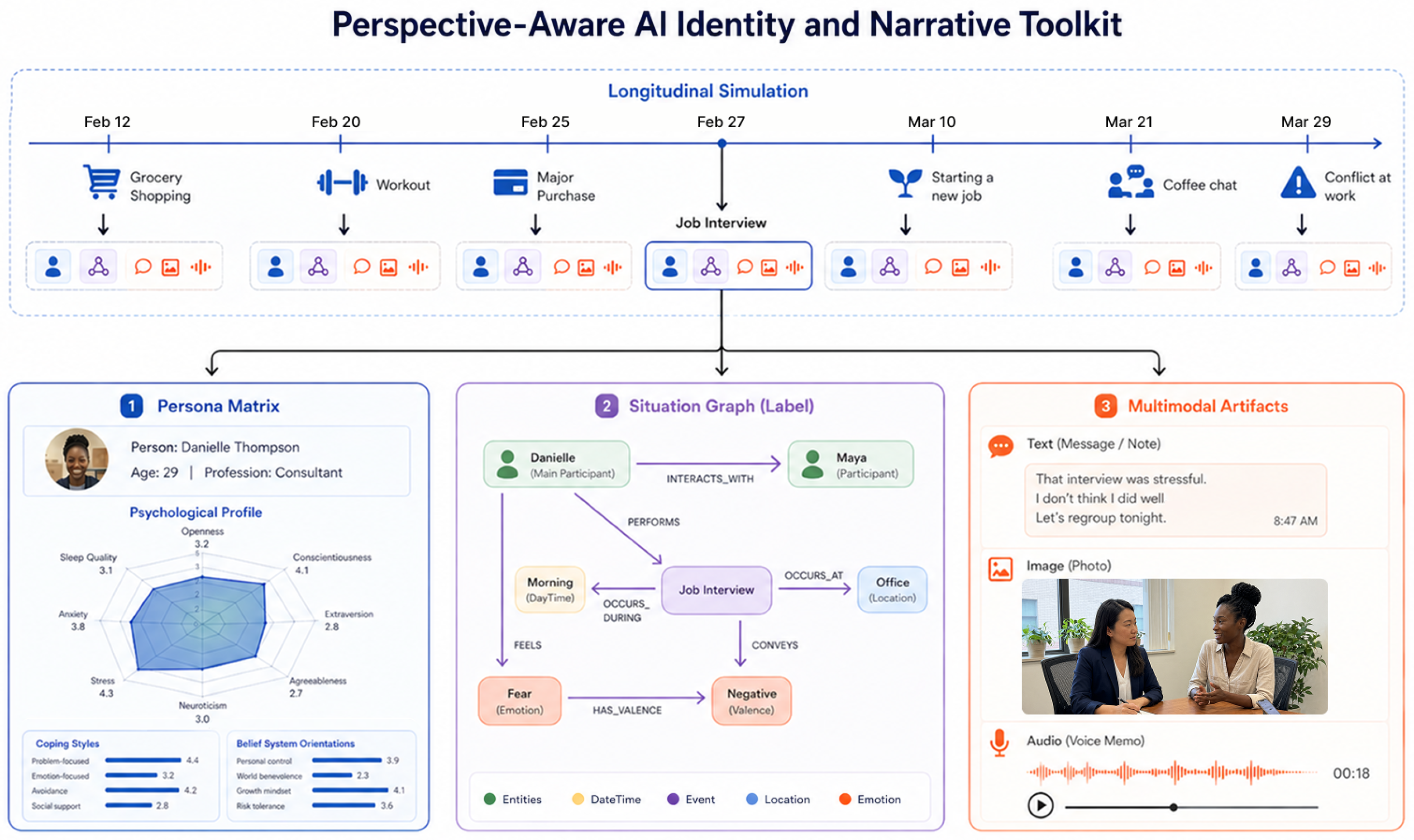
Figure 1.
The structured Persona Matrix (1), the ontology-aligned Situation Graph label (2), and the generated multimodal artifacts (3), evolving longitudinally. The Situation Graph serves as a supervised signal for downstream inference tasks, while multimodal artifacts are conditioned cross-modally on the unified situation state.
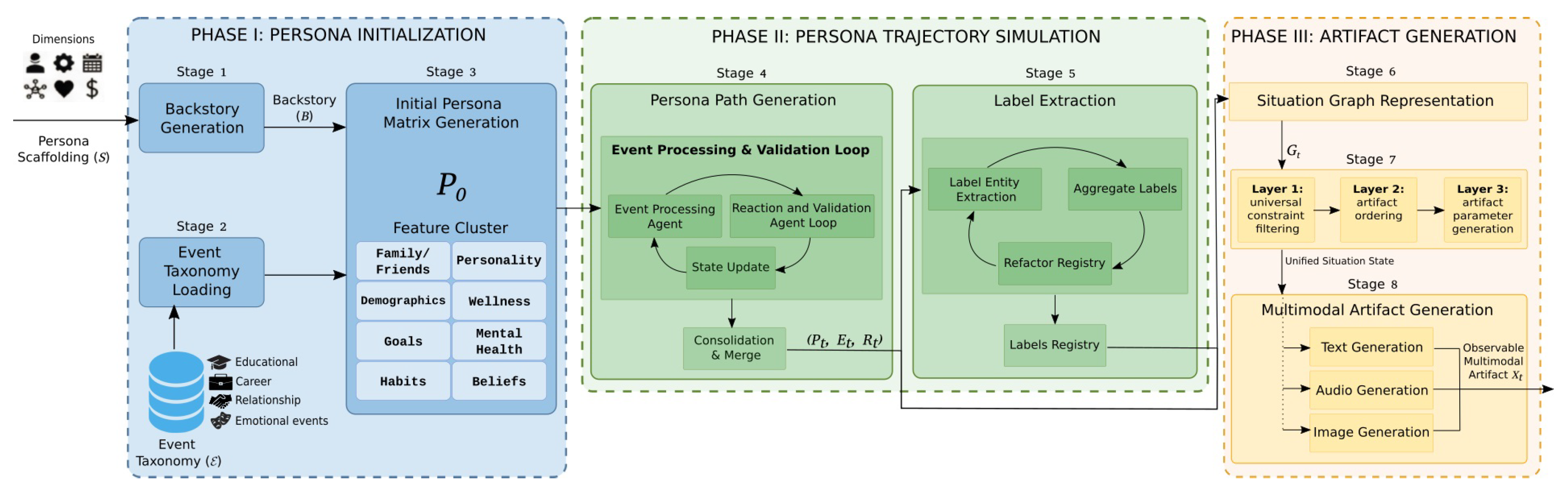
Figure 2.
PAiNT workflow across Stages 1–8. The pipeline proceeds from persona initialization (Stages 1–3), to trajectory simulation (Stages 4–5), to Situation Graph and multimodal artifact generation (Stages 6–8), while maintaining explicit identity state and structural supervision throughout.
Figure 2.
PAiNT workflow across Stages 1–8. The pipeline proceeds from persona initialization (Stages 1–3), to trajectory simulation (Stages 4–5), to Situation Graph and multimodal artifact generation (Stages 6–8), while maintaining explicit identity state and structural supervision throughout.
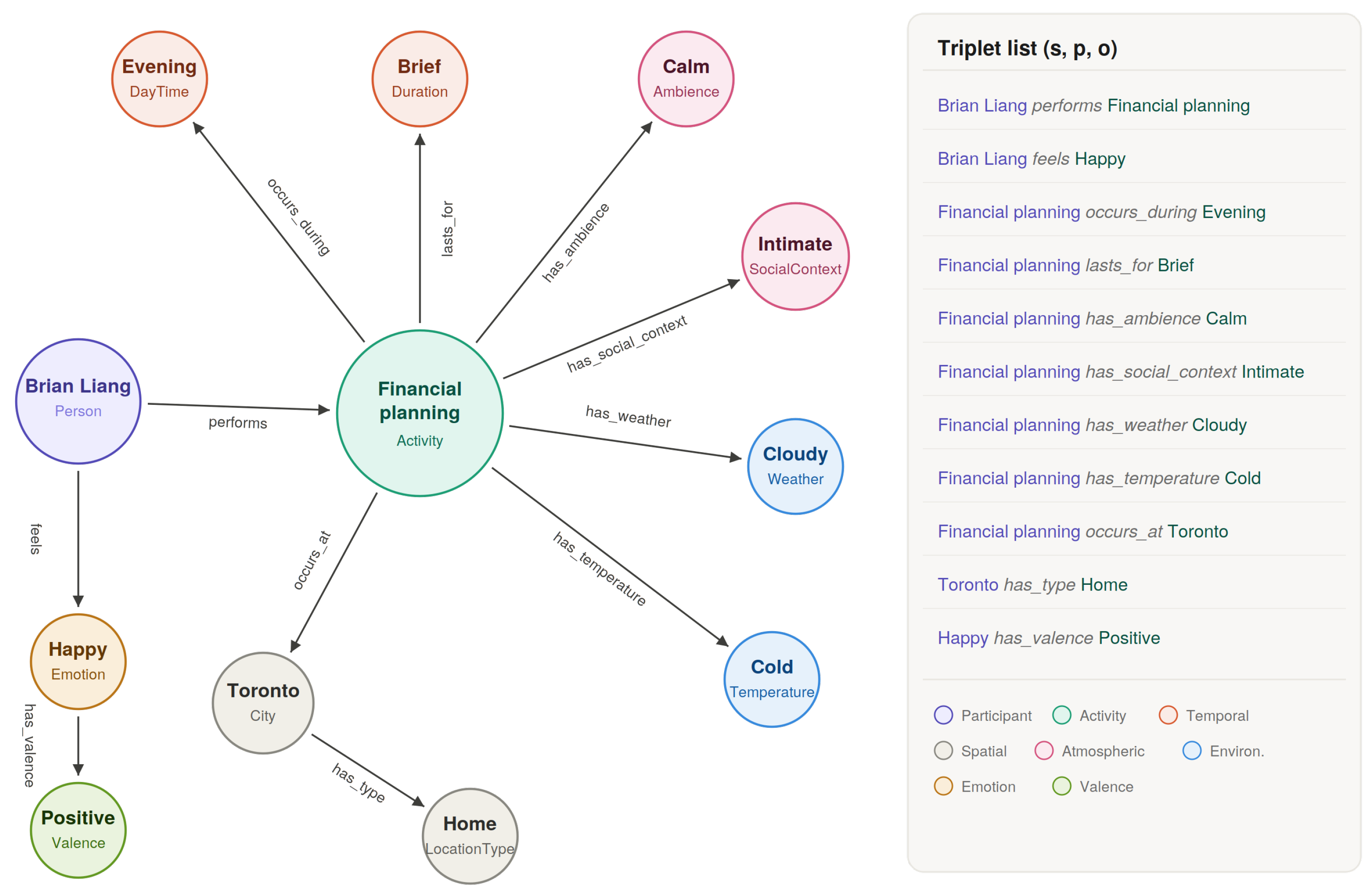
Figure 3.
Example Situation Graph for a single timestep (Brian Liang, : financial planning). The left panel shows the graph structure with the Activity node as the central hub and typed edges radiating to spatiotemporal, atmospheric, environmental, and psychological nodes. The right panel lists all triplets comprising .
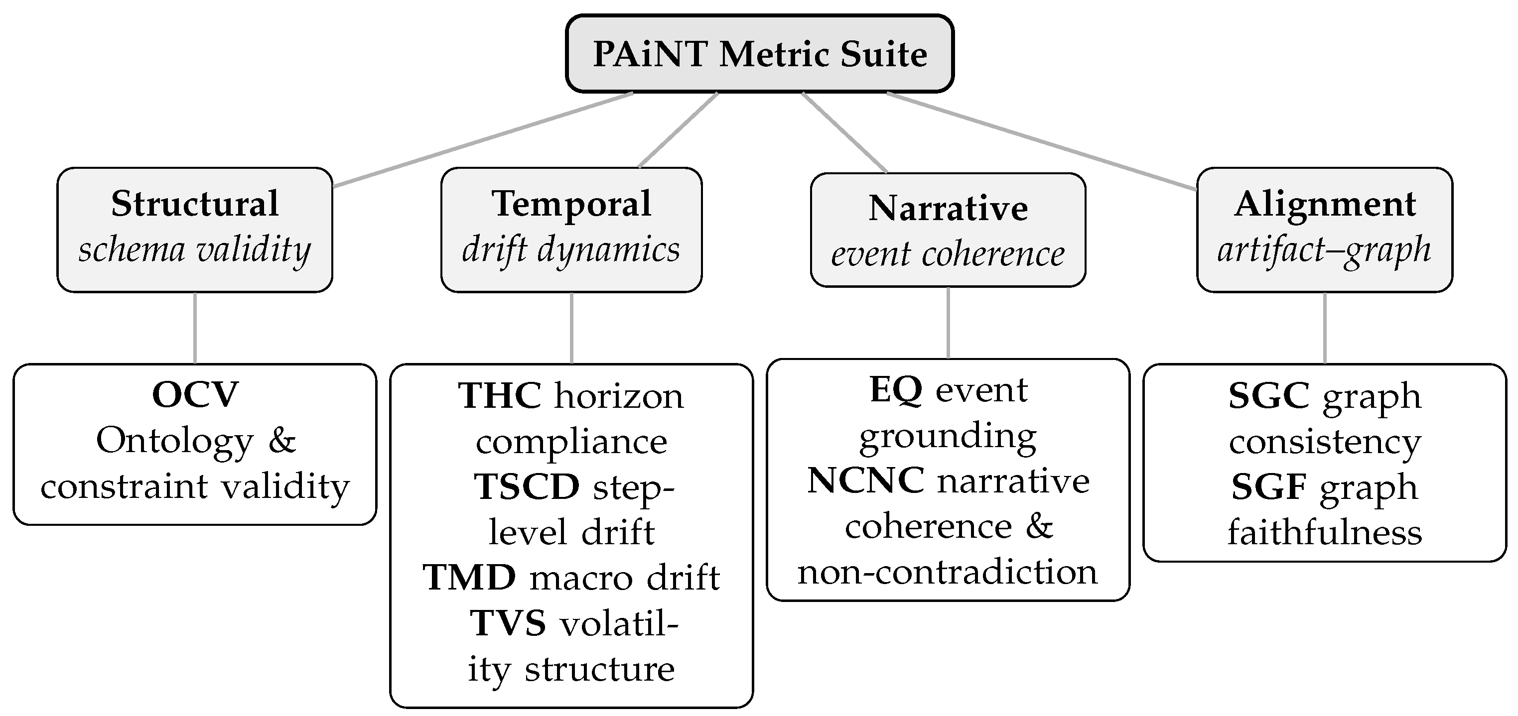
Figure 4.
Overview of the PAiNT metric suite, organized by what each metric evaluates.
Structural metrics check schema well-formedness. This complements the per-metric definitions in
Table 4.
Figure 4.
Overview of the PAiNT metric suite, organized by what each metric evaluates.
Structural metrics check schema well-formedness. This complements the per-metric definitions in
Table 4.
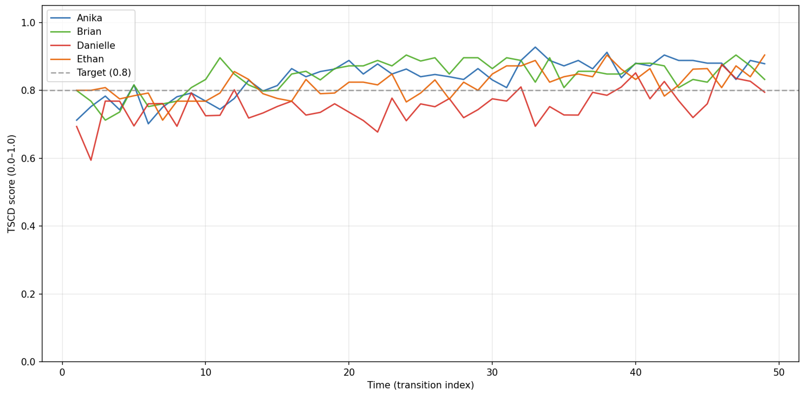
Figure 5.
Temporal stability floor: mean TSCD per archetype over 50 transitions. Dashed line marks the 0.80 reference level. Danielle (Self-centered) shows the most frequent rate-cap violations. Overall mean = 0.814.
Figure 5.
Temporal stability floor: mean TSCD per archetype over 50 transitions. Dashed line marks the 0.80 reference level. Danielle (Self-centered) shows the most frequent rate-cap violations. Overall mean = 0.814.
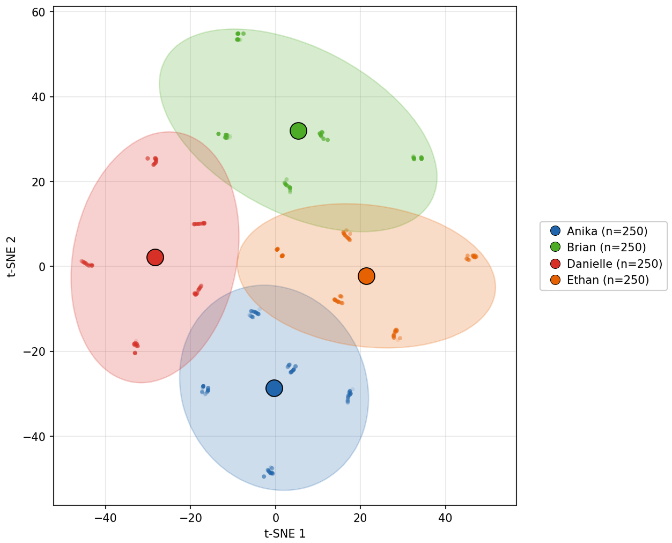
Figure 6.
Identity persistence in state space (t-SNE, perplexity = 40,
). Each point is one timestep-level Persona Matrix (
). Color encodes archetype. Sub-trajectories from independent seeds form coherent paths within each archetype region. The Brian–Ethan overlap is attributable to shared demographic encodings (
Table 6).
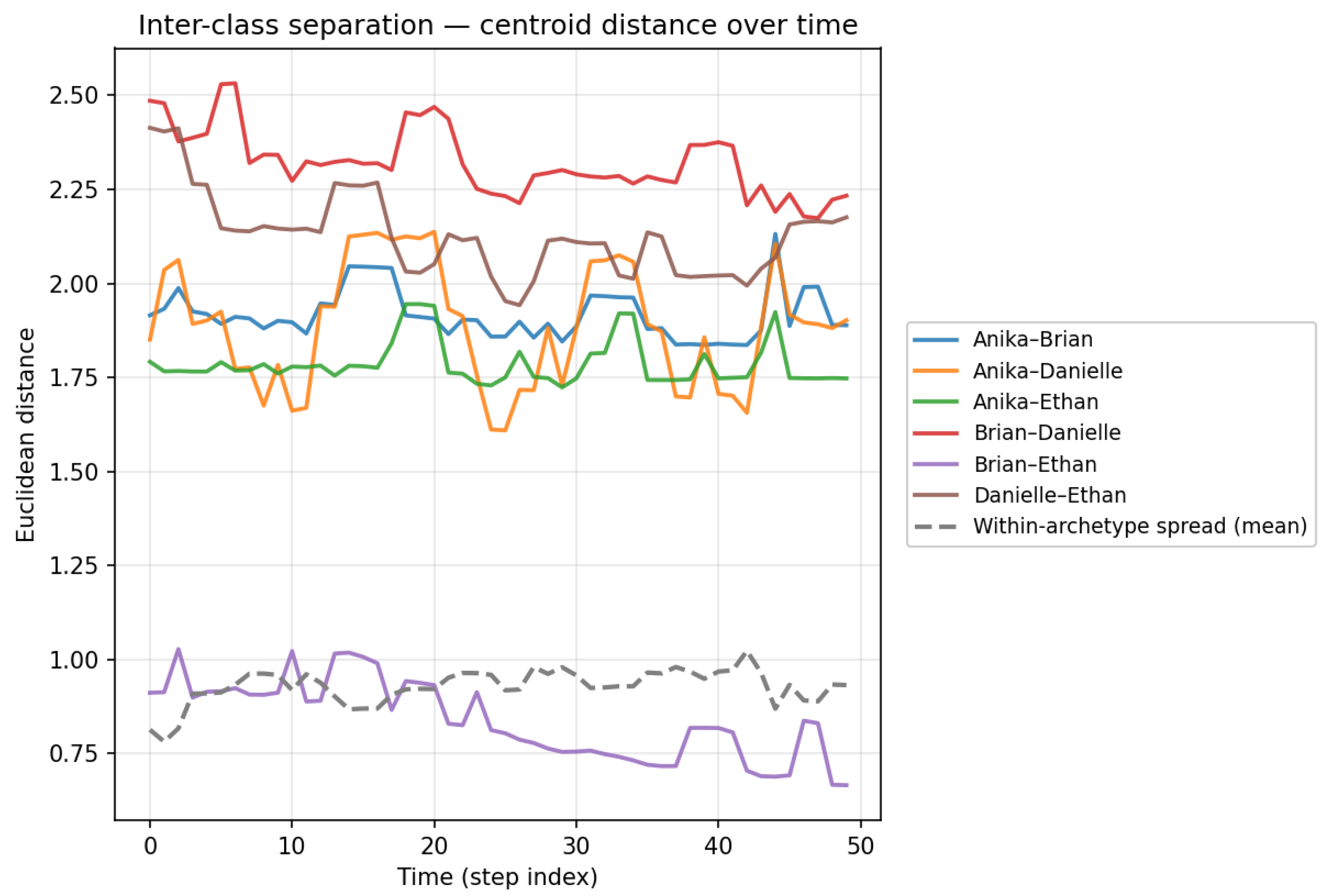
Figure 7.
Inter-class separation over time. Solid lines: pairwise centroid distances; dashed line: mean within-archetype spread. The identity signal persists above stochastic noise throughout, including at the terminal timestep.
Figure 7.
Inter-class separation over time. Solid lines: pairwise centroid distances; dashed line: mean within-archetype spread. The identity signal persists above stochastic noise throughout, including at the terminal timestep.
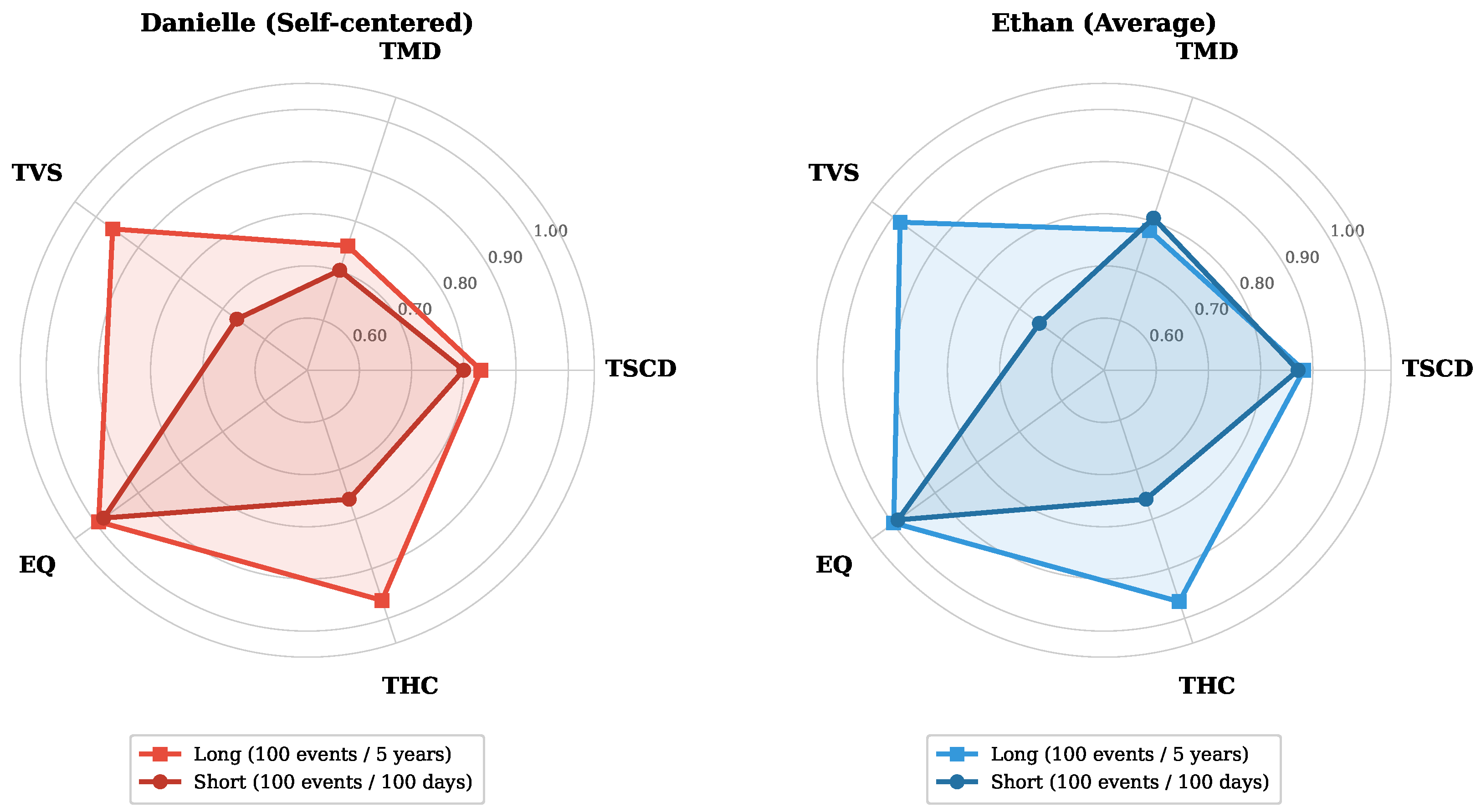
Figure 8.
The coherence frontier under short-horizon (100 events/100 days, dark) and long-horizon (100 events/5 years, light) conditions for two archetypes. The short-horizon polygon contracts most strongly on TVS and THC, indicating that the frontier is driven primarily by resolution-sensitive temporal dimensions rather than uniform quality degradation. Danielle’s short-horizon profile is also more distorted than Ethan’s, consistent with higher archetype volatility amplifying compression sensitivity.
Figure 9.
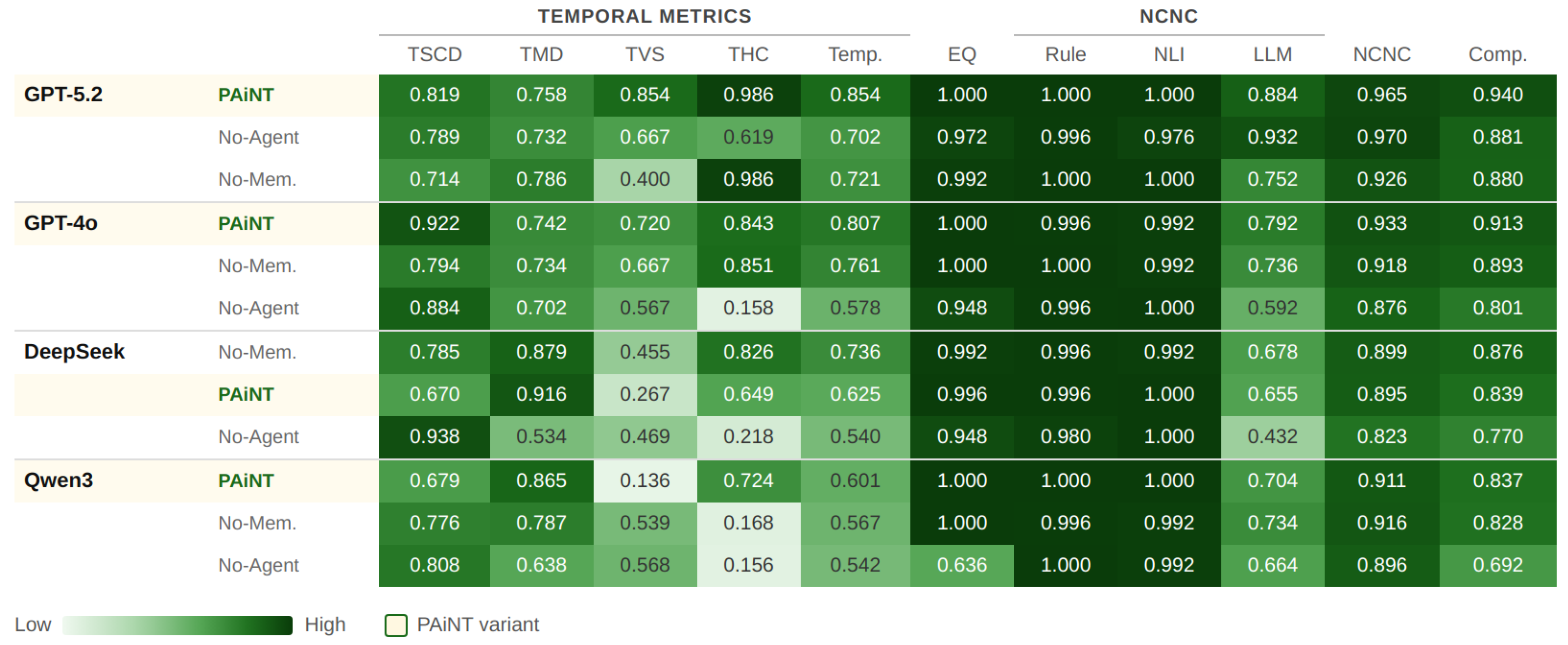
Experiment 3: Full per-metric breakdown. Color intensity encodes score magnitude (darker = higher). All values are means over
seeds. Full numerical results are reported in
Table A5 in
Appendix G.
Figure 9.
Experiment 3: Full per-metric breakdown. Color intensity encodes score magnitude (darker = higher). All values are means over
seeds. Full numerical results are reported in
Table A5 in
Appendix G.
Figure 10.
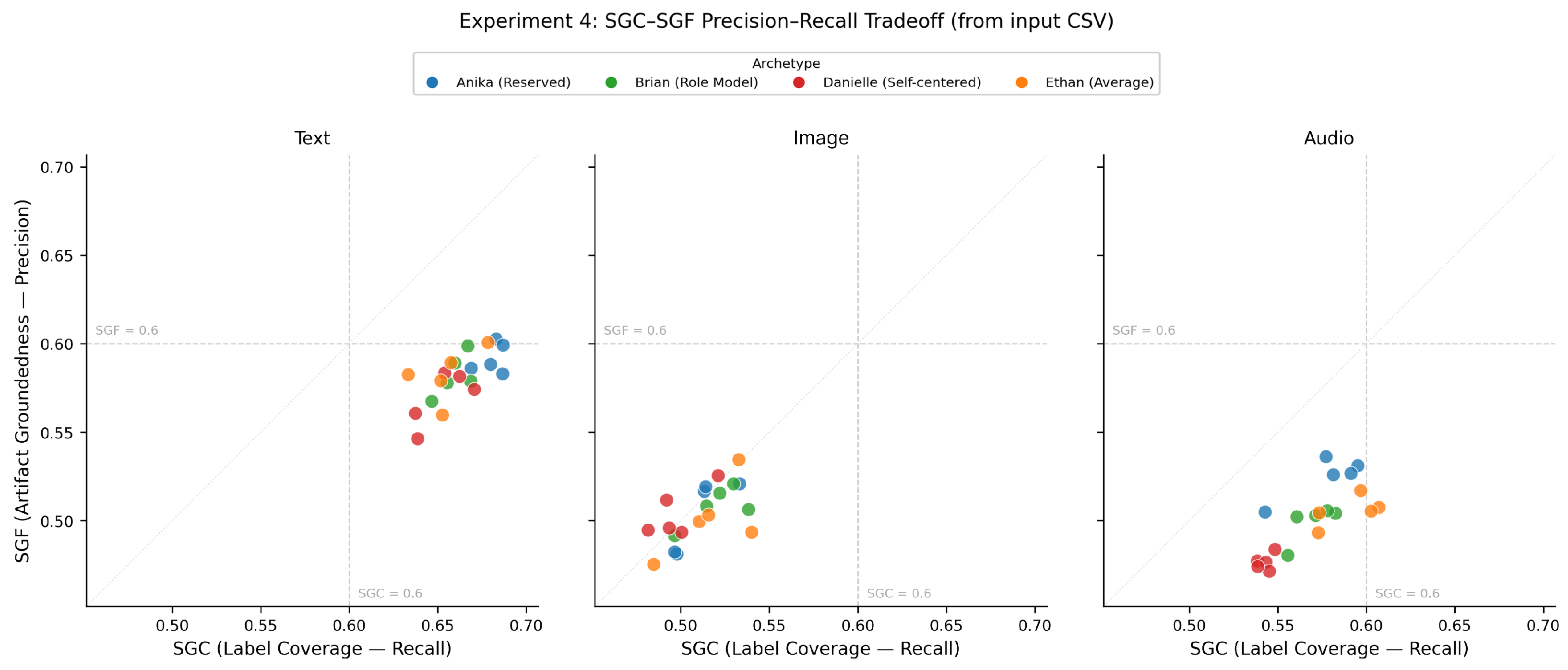
SGC–SGF relationship by modality. Each point is one archetype–seed run. The positive association indicates that better artifacts tend to be both more comprehensive and more grounded, rather than trading one property off against the other. Text artifacts cluster closest to the upper-right region.
Figure 11.
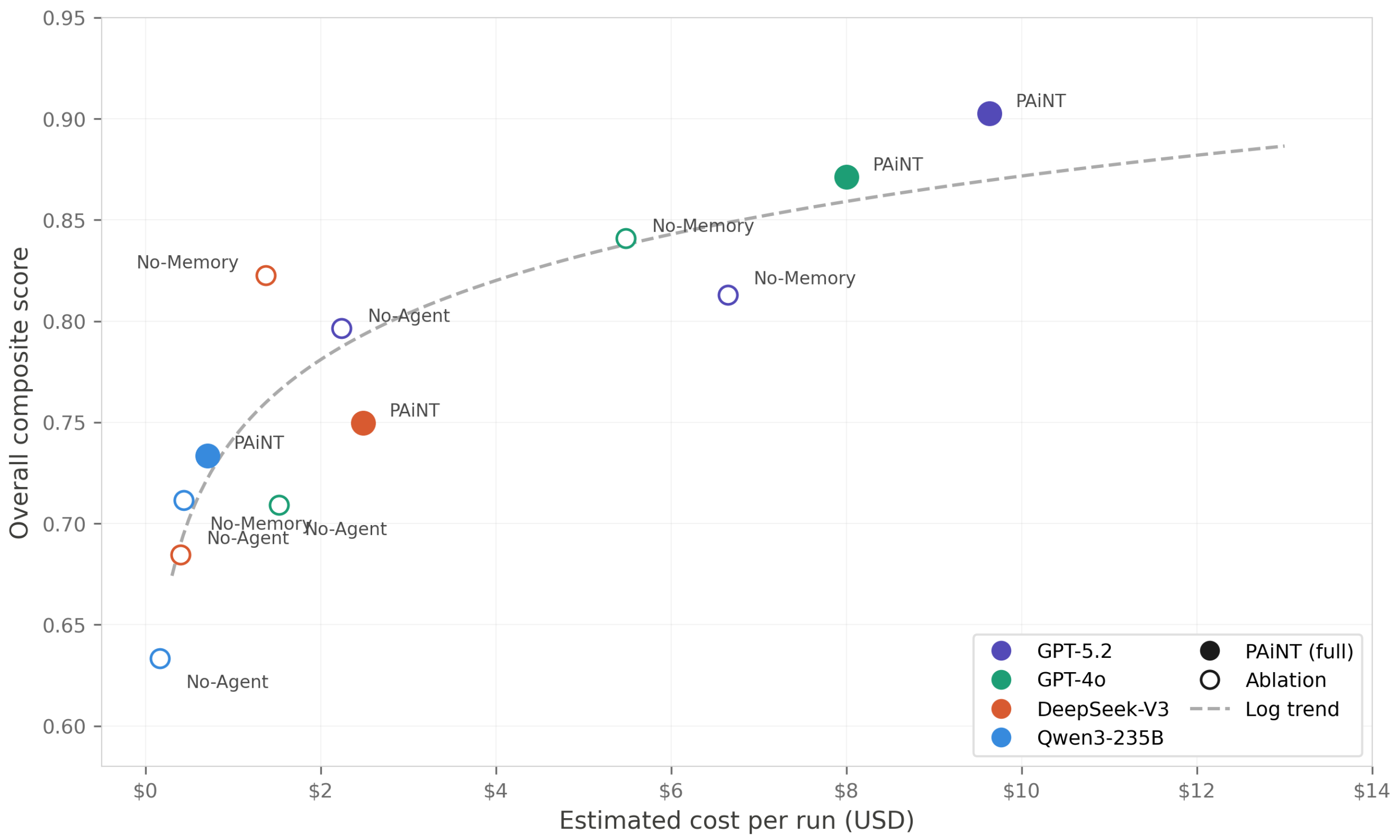
Cost–quality trade-off across backbones and architectural variants (Stages 1–4, events, seeds per condition). Cost is estimated from mean per-run token counts at API rates as of April 2026.
Figure 11.
Cost–quality trade-off across backbones and architectural variants (Stages 1–4, events, seeds per condition). Cost is estimated from mean per-run token counts at API rates as of April 2026.
Figure 12.
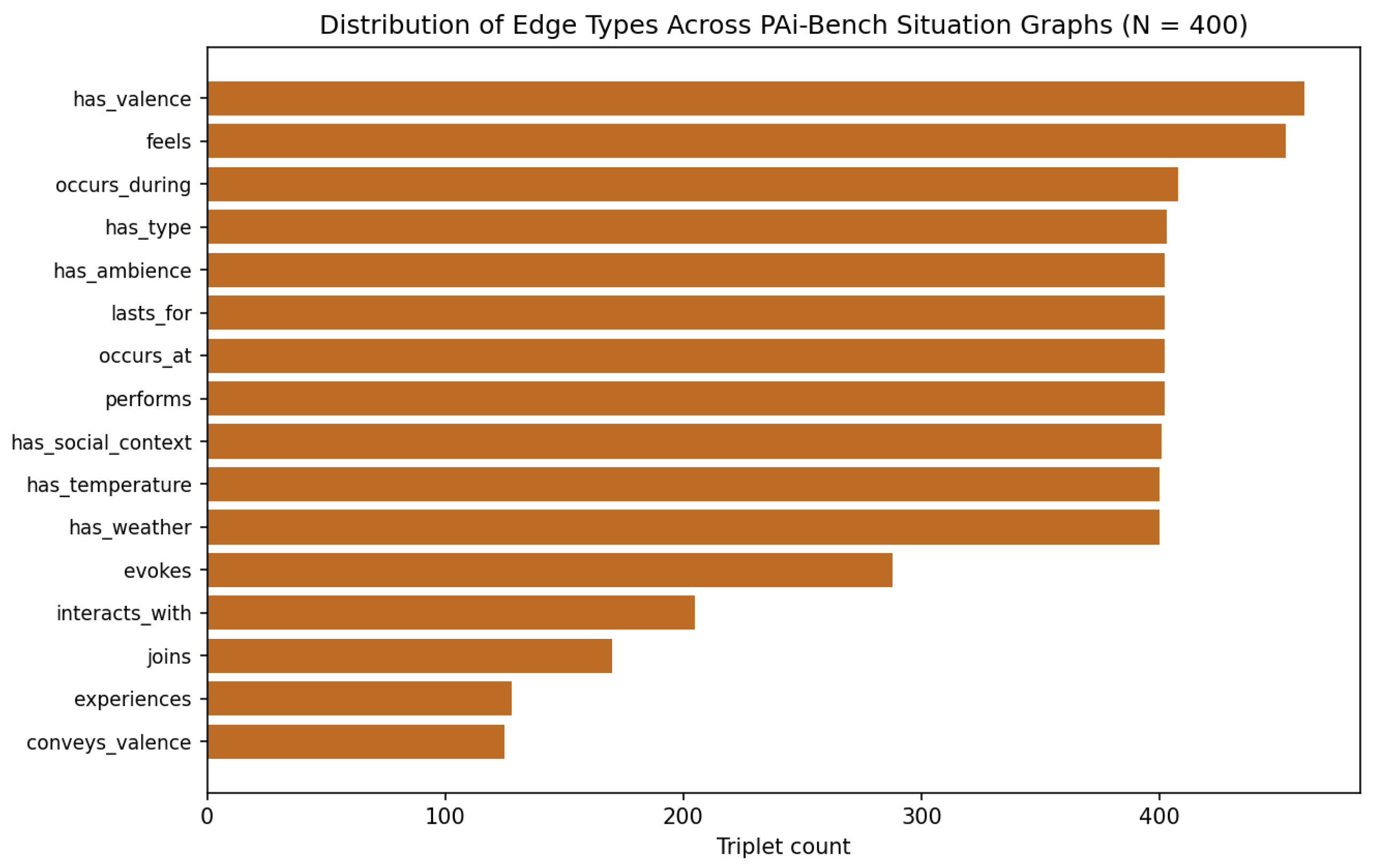
Distribution of edge types across all 400 PAi-Bench Situation Graphs. Edge types appearing in every graph (has_valence, feels, occurs_during, and core spatiotemporal predicates) approach the maximum of 400 triplets, while social and psychological edges (interacts_with, joins, experiences, conveys_valence) are sparser, reflecting their conditional role in the schema.
Figure 13.
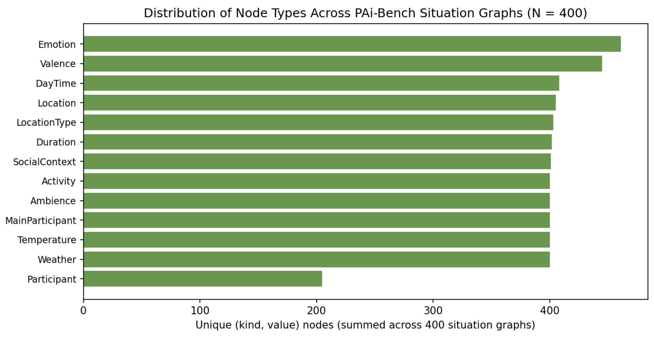
Distribution of node types by unique (kind, value) pair count across all 400 PAi-Bench Situation Graphs. All required node types approach 400, confirming schema compliance. Participant is the only node type substantially below this ceiling, reflecting its optional and persona-dependent role. The slight excess of Emotion and Valence above 400 indicates that a subset of graphs encodes multiple co-occurring emotional states.
Figure 14.
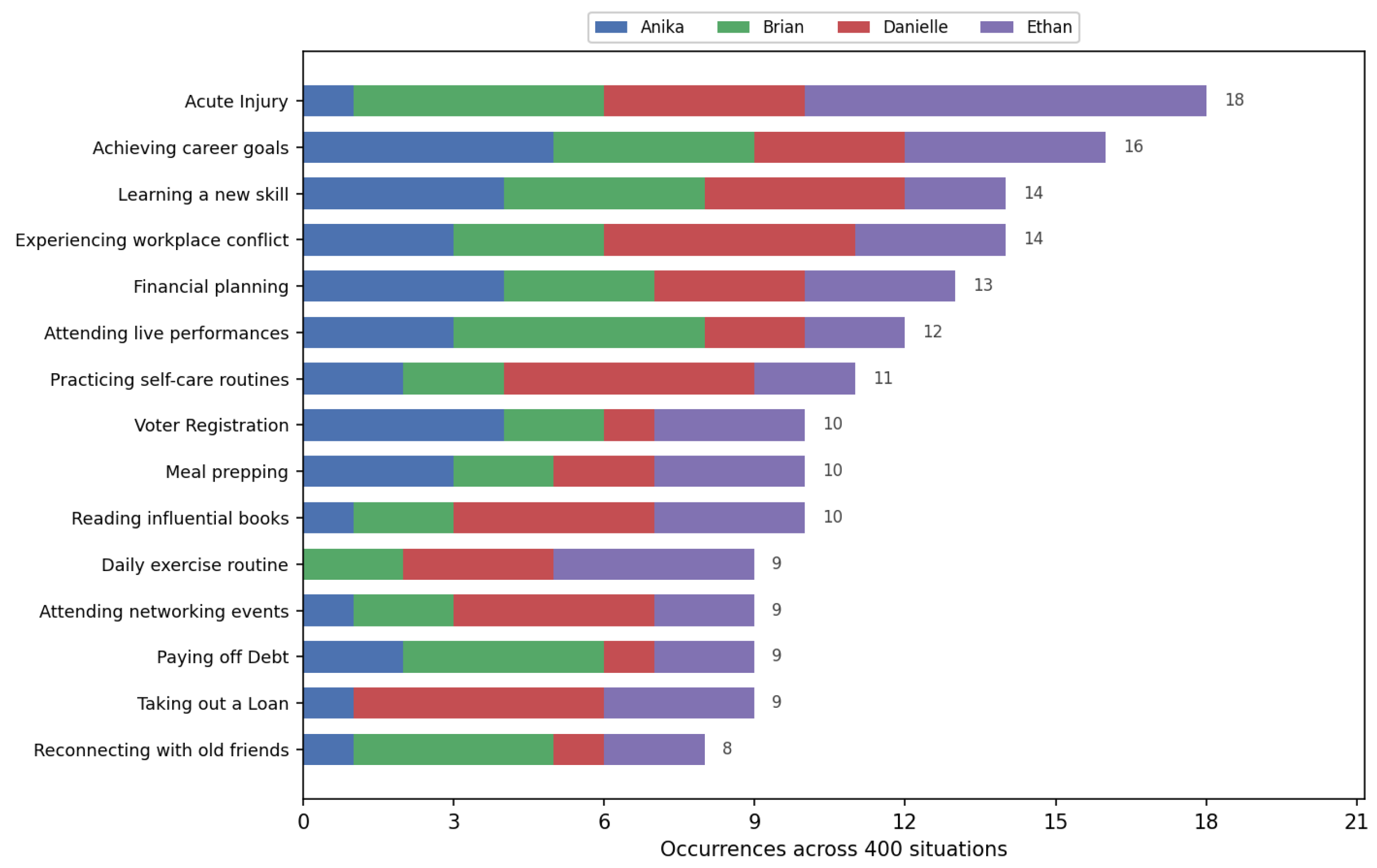
Top 15 most frequent event titles in PAi-Bench, stacked by archetype ( total event occurrences). A small shared core of life events appears across personas, while the long tail (71 further titles, not shown) captures archetype-specific behavior.
Figure 14.
Top 15 most frequent event titles in PAi-Bench, stacked by archetype ( total event occurrences). A small shared core of life events appears across personas, while the long tail (71 further titles, not shown) captures archetype-specific behavior.
Figure 15.
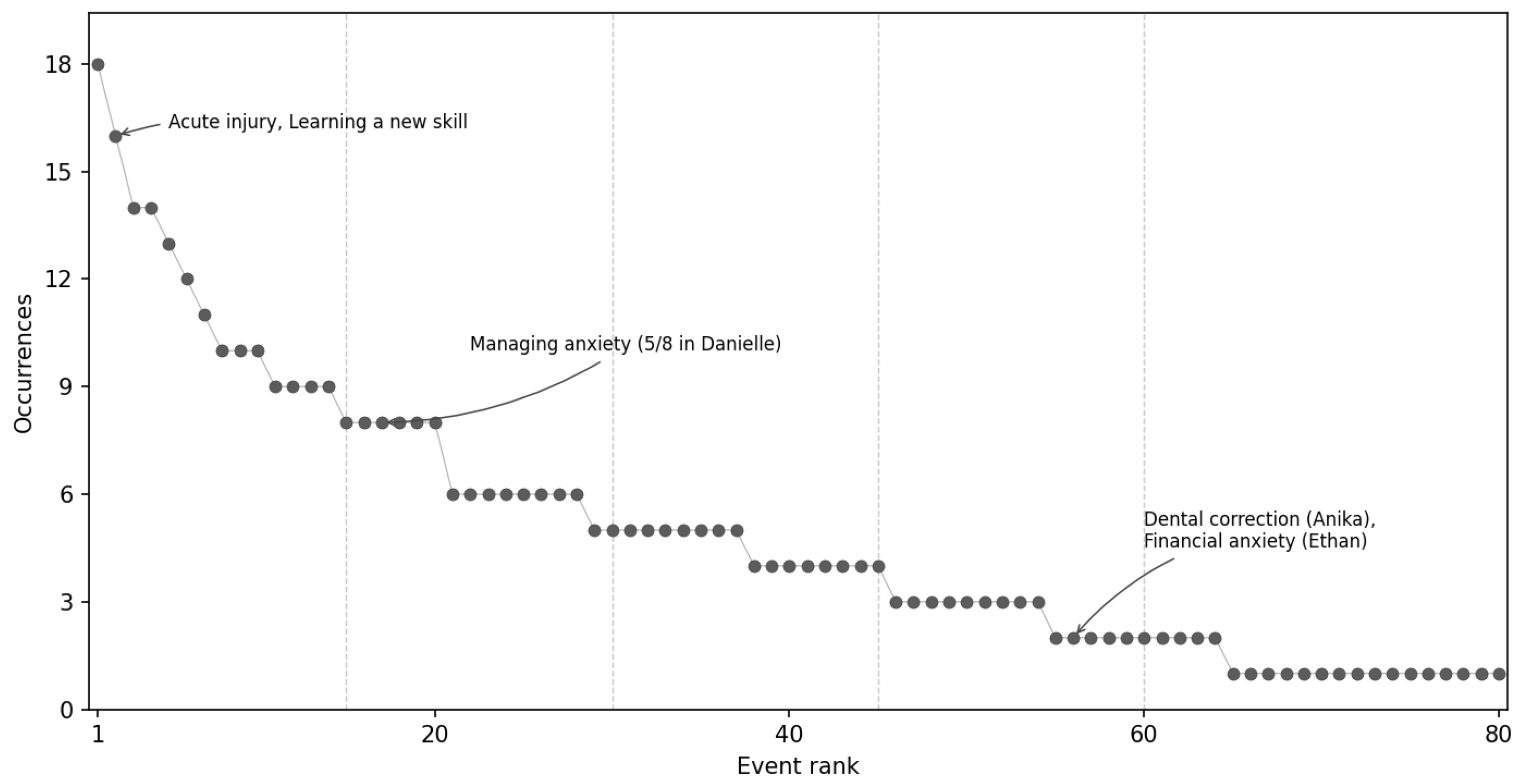
Event frequency distribution in PAi-Bench, ranked by total occurrences across all 400 situations (80 distinct titles drawn from the 260-event PAiNT taxonomy).
Figure 15.
Event frequency distribution in PAi-Bench, ranked by total occurrences across all 400 situations (80 distinct titles drawn from the 260-event PAiNT taxonomy).
Figure 16.
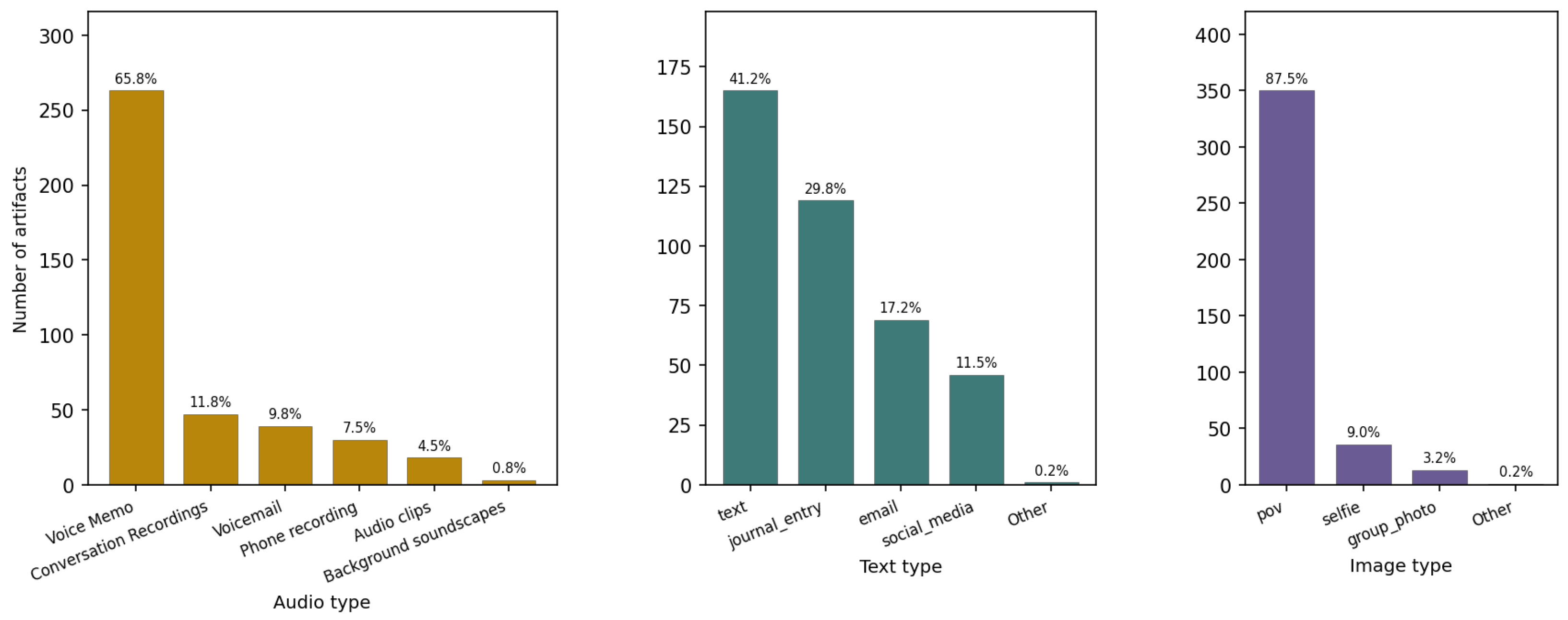
Artifact modality distributions across the 400 situations in PAi-Bench. Audio artifacts (left) are dominated by voice memos (); text artifacts (center) skew toward short-form messages () and journal entries (); image artifacts (right) are overwhelmingly point-of-view shots (). The first-person skew across all three modalities is intentional and reflects the design goal of modeling artifacts that a real user could plausibly originate over time.
Figure 17.
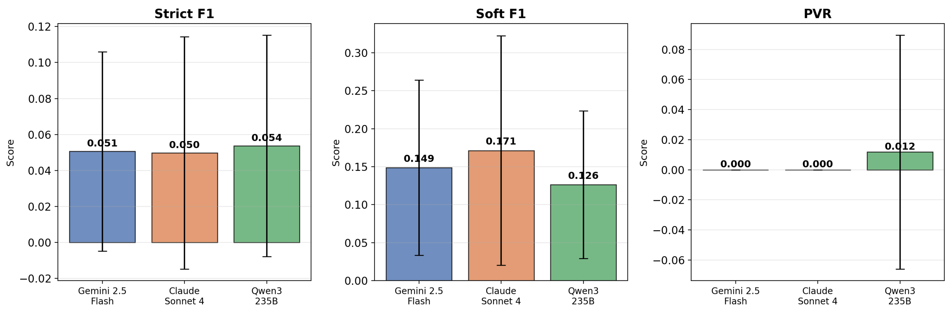
Overall performance comparison across three models. Strict F1 is uniformly low (∼0.05) across all models, reflecting the difficulty of exact string matching on free-form values (activity descriptions, person names, location types). Soft F1 reveals meaningful separation: Claude Sonnet 4 leads (0.171), followed by Gemini 2.5 Flash (0.149) and Qwen3-235B (0.126). PVR is zero for both proprietary models; Qwen3 exhibits minor ontology violations (0.012).
Figure 18.
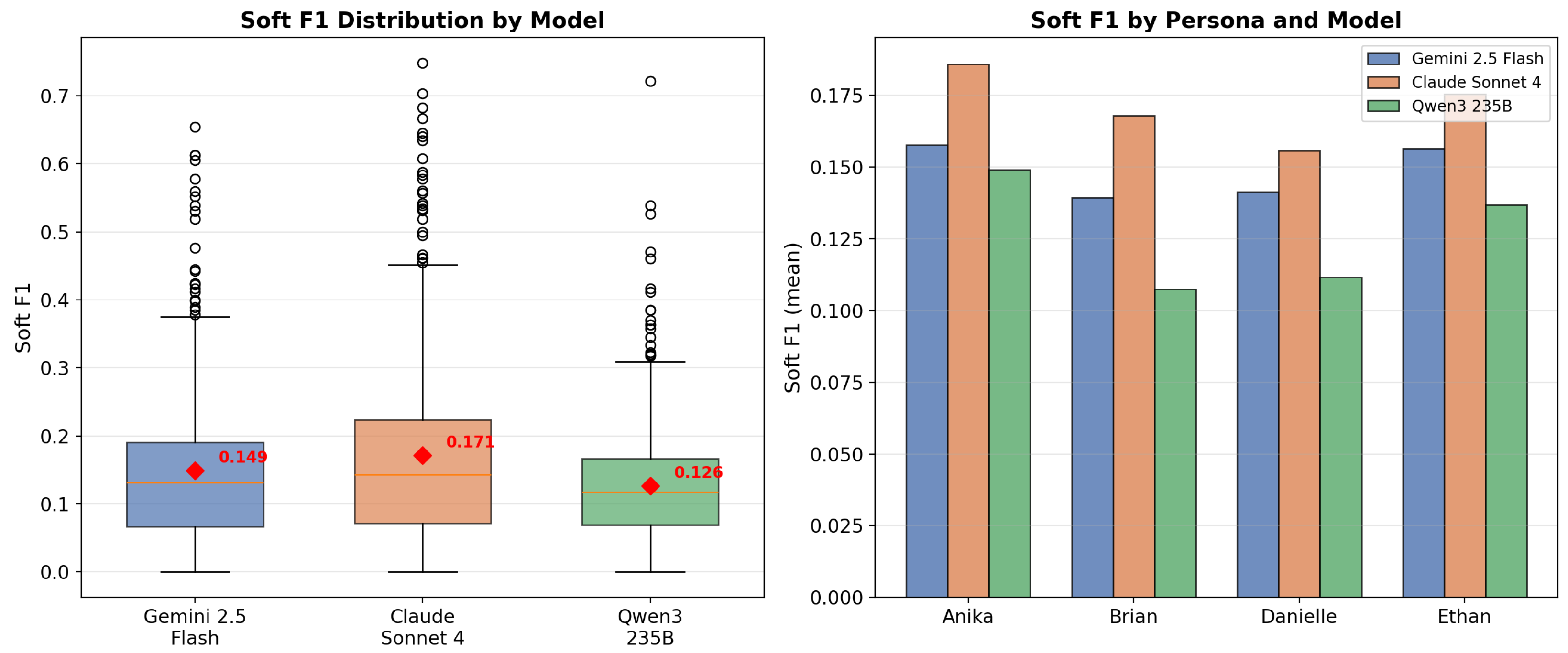
(Left): Soft F1 score distributions by model. All three exhibit right-skewed distributions with long tails, indicating a majority of events score below 0.2 with a minority achieving moderate performance (>0.3). Claude shows the widest spread, suggesting greater variance in prediction quality. (Right): Per-persona Soft F1 means. Performance is consistent across personas within each model, indicating the task difficulty is driven by the inference challenge rather than persona-specific content.
Table 1.
Comparison of PAiNT with representative persona-simulation and user-modeling frameworks across five capability axes.
Table 1.
Comparison of PAiNT with representative persona-simulation and user-modeling frameworks across five capability axes.
| Framework | State
Representation | Explicit &
Inspectable State | Longitudinal
Modeling | Supervision
(GT Labels) | Multimodal
Generation | Downstream
Learning |
|---|
| Persona-Chat [8] | Textual description | ✗ | ✗ | ✗ | ✗ | ✗ |
| PersonaHub [13] | Textual/attribute | ✗ | ✗ | ✗ | ✗ | Partial |
| Generative Agents [11] | Implicit stream | ✗ | ✓ (impl.) | ✗ | ✗ | ✗ |
| User-LLM [16] | Embedding | ✗ | ✓ | ✗ | ✗ | ✓ |
| DeepPersona [14] | Structured attribute | ✗ | ✗ | ✗ | ✗ | Partial |
| PAiNT (ours) | Explicit structured | ✓ | ✓ | ✓ | ✓ | ✓ |
Table 2.
Situation Graph node types (), their type-specific entity enumerations (), and allowed values. Closed: the value is fully determined by . Open: the value is drawn from the finite, persona-specific label registry produced by Stage 5 and populated by the Autolabeler in Stage 6.
Table 2.
Situation Graph node types (), their type-specific entity enumerations (), and allowed values. Closed: the value is fully determined by . Open: the value is drawn from the finite, persona-specific label registry produced by Stage 5 and populated by the Autolabeler in Stage 6.
| Node Type () | Allowed Entities () | Allowed Values |
|---|
| MainParticipant | {Person} | Open (value from Stage 5) |
| Participant | {FamilyMember, Friend, RomanticPartner, Acquaintance} | Open (value from Stage 5) |
| Activity | {Activity} | Open (value from via Stage 5) |
| Location | {Global, Country, Region, City} | Open (value from Stage 5) |
| LocationType | {Home, Work, School, Park, Restaurant, Cafe, Hotel, Airport, Gym, Beach, Theatre, Museum, Library} | Open (value from Stage 5) |
| DayTime | {Morning, Afternoon, Evening, Night} | Closed (value ) |
| Duration | {Brief, FewHours, HalfDay, FullDay} | Closed (value ) |
| Ambience | {Serene, Cozy, Vibrant, Chaotic, Mysterious, Majestic, Bleak, Romantic, Calm} | Closed (value ) |
| SocialContext | {Intimate, Casual, SemiFormal, Professional, Ceremonial} | Closed (value ) |
| Weather | {Rainy, Sunny, Snowy, Cloudy, Foggy, Windy, Stormy} | Closed (value ) |
| Temperature | {Hot, Warm, Cool, Cold, Freezing} | Closed (value ) |
| Emotion | {Happy, Sad, Fear, Disgust, Anger, Surprise} | Closed (value ) |
| Valence | {Positive, Negative} | Closed (value ) |
Table 3.
Situation Graph constraint map: complete set of valid (source kind → target kind) pairs for each of the 16 edge types. The five semantic edge groups—core action, spatiotemporal, atmospheric, environmental, and psychological—were designed to cover the canonical dimensions of human situation representation identified in cognitive science [
33,
34].
| Semantic Group | Edge Type (p) | Valid |
|---|
| Core action | performs | MainParticipant → Activity |
| experiences | MainParticipant → Activity; Participant → Activity |
| joins | Participant → Activity |
| interacts_with | MainParticipant → Participant; Participant → MainParticipant; Participant → Participant |
| Spatiotemporal | occurs_at | Activity → Location |
| has_type | Location → LocationType |
| occurs_during | Activity → DayTime |
| lasts_for | Activity → Duration |
| Atmospheric | has_ambience | Activity → Ambience; Location → Ambience |
| has_social_context | Activity → SocialContext; Location → SocialContext |
| Environmental | has_weather | Activity → Weather |
| has_temperature | Activity → Temperature |
| Psychological | feels | MainParticipant → Emotion; Participant → Emotion |
| has_valence | Emotion → Valence |
| evokes | Activity → Emotion |
| conveys_valence | Activity → Valence |
Table 4.
Summary of the PAiNT evaluation metrics. The suite includes constraint-satisfaction metrics, which function as validity checks, and characterization metrics, which support comparative analysis across experiments.
Table 4.
Summary of the PAiNT evaluation metrics. The suite includes constraint-satisfaction metrics, which function as validity checks, and characterization metrics, which support comparative analysis across experiments.
| Metric | Definition |
|---|
| Category: Persona Representation Quality |
| Structural |
| OCV: Ontology & Constraint Validity | Checks whether each Persona Matrix satisfies the schema and ontology constraints (field types, value ranges, invariants). |
| Temporal |
| TSCD: Temporal Smoothness & Controlled Drift | Detects implausibly large per-step attribute changes using calibrated daily rate caps and hard absolute ceilings. |
| TMD: Temporal Macro Drift | Detects generative stagnation by measuring cumulative drift budget utilization for state-like attributes across the full trajectory. |
| TVS: Temporal Volatility Structure | Evaluates whether the distributional pattern of step-level drift activity exhibits structured variability—neither mechanically uniform nor chaotically erratic. |
| THC: Temporal Horizon Compliance | Evaluates whether the generated trajectory respects the configured
simulation horizon, penalizing both temporal undershoot and overshoot
with an asymmetric band-pass scoring function. |
| Event-Driven |
| EQ: Event Quality | Measures the fraction of sampled events that appear in the canonical Event Taxonomy, detecting event hallucination. |
| NCNC: Narrative Coherence & Non-Contradiction | Assesses logical consistency of the event timeline using rule-based prerequisite checks, attribute-scoped NLI contradiction detection, and an LLM-based narrative plausibility audit. |
| Category: Distributional & Stability Diagnostics |
| Silhouette Score (Inter-Class Separation) | Quantifies how well Persona Matrices cluster by archetype in identity state space using the mean silhouette coefficient. |
| Final-State Spread (Intra-Class Stability) | Measures within-archetype dispersion of terminal identity states across stochastic seeds using mean Euclidean distance to the archetype centroid. |
| Category: Artifact–Graph Alignment |
| SGC: Situation Graph Consistency | Evaluates whether generated artifacts entail (and do not contradict) facts encoded in the corresponding Situation Graph. |
| SGF: Situation Graph Faithfulness | Evaluates whether facts asserted by generated artifacts are grounded in the corresponding Situation Graph, penalizing contradictions and treating ungrounded elaboration as neutral. |
Table 5.
Experiment 1 summary. All trajectories generated with GPT-5.2.
Table 5.
Experiment 1 summary. All trajectories generated with GPT-5.2.
| | | | Per-Archetype |
|---|
|
Metric
|
Claims
|
Overall
|
Anika
|
Brian
|
Danielle
|
Ethan
|
|---|
| TSCD | C1 | 0.814 | 0.838 | 0.843 | 0.755 | 0.819 |
| Silhouette Score | C2 | 0.269 | 0.273 | 0.113 | 0.443 | 0.246 |
| Final Spread | C3 | 0.932 | 1.138 | 0.881 | 0.961 | 0.746 |
Table 6.
Pairwise centroid distance decomposition by sub-vector component, sorted by full distance (descending).
Table 6.
Pairwise centroid distance decomposition by sub-vector component, sorted by full distance (descending).
| Pair | Full | Core | Fixed | Narrative |
|---|
| Brian–Danielle | 2.279 | 1.440 | 1.727 | 0.369 |
| Danielle–Ethan | 2.087 | 1.086 | 1.746 | 0.375 |
| Anika–Brian | 1.881 | 0.829 | 1.651 | 0.356 |
| Anika–Danielle | 1.846 | 1.313 | 1.254 | 0.355 |
| Anika–Ethan | 1.755 | 0.533 | 1.648 | 0.282 |
| Brian–Ethan | 0.754 | 0.604 | 0.328 | 0.306 |
Table 7.
Inter-archetype silhouette under the full Identity State Vector versus a reduced vector with the fixed-identity (demographic one-hot) sub-vector removed. Mean silhouette coefficient (Euclidean), per archetype, .
Table 7.
Inter-archetype silhouette under the full Identity State Vector versus a reduced vector with the fixed-identity (demographic one-hot) sub-vector removed. Mean silhouette coefficient (Euclidean), per archetype, .
| Archetype | Full | Reduced | |
|---|
| Anika | 0.273 | 0.451 | |
| Brian | 0.113 | 0.513 | |
| Danielle | 0.443 | 0.469 | |
| Ethan | 0.246 | 0.173 | |
| Overall | 0.269 | 0.401 | +0.133 |
Table 8.
Experiment 2: Mean metric scores by archetype and horizon ( seeds per condition). All generated with GPT-5.2.
Table 8.
Experiment 2: Mean metric scores by archetype and horizon ( seeds per condition). All generated with GPT-5.2.
| Archetype | Horizon | TSCD | TMD | TVS | EQ | THC | Composite |
|---|
| Danielle | short | 0.800 ± 0.02 | 0.701 ± 0.11 | 0.667 ± 0.00 | 0.982 ± 0.01 | 0.760 ± 0.00 | 0.818 ± 0.02 |
| Danielle | long | 0.833 ± 0.03 | 0.751 ± 0.11 | 0.961 ± 0.09 | 0.994 ± 0.01 | 0.964 ± 0.01 | 0.917 ± 0.02 |
| Ethan | short | 0.872 ± 0.03 | 0.807 ± 0.01 | 0.653 ± 0.02 | 0.988 ± 0.01 | 0.760 ± 0.00 | 0.846 ± 0.01 |
| Ethan | long | 0.882 ± 0.02 | 0.781 ± 0.04 | 0.983 ± 0.02 | 0.998 ± 0.00 | 0.966 ± 0.01 | 0.935 ± 0.01 |
Table 9.
Experiment 2: Conditions ranked by Composite score.
Table 9.
Experiment 2: Conditions ranked by Composite score.
| Rank | Horizon | Persona | Composite |
|---|
| 1 | long | Ethan | 0.935 |
| 2 | long | Danielle | 0.917 |
| 3 | short | Ethan | 0.846 |
| 4 | short | Danielle | 0.818 |
Table 10.
Experiment 2: NCNC scores by archetype and horizon (mean ± std, ). All generated with GPT-5.2.
Table 10.
Experiment 2: NCNC scores by archetype and horizon (mean ± std, ). All generated with GPT-5.2.
| | | Rule | NLI | LLM | Combined |
|---|
|
Archetype
|
Horizon
| Mean | Std | Mean | Std | Mean | Std | Mean | Std |
|---|
| Danielle | long | 1.000 | 0.00 | 0.998 | 0.00 | 0.932 | 0.05 | 0.979 | 0.01 |
| Danielle | short | 0.998 | 0.00 | 0.994 | 0.01 | 0.790 | 0.12 | 0.934 | 0.04 |
| Ethan | long | 0.998 | 0.00 | 0.988 | 0.01 | 0.870 | 0.09 | 0.956 | 0.02 |
| Ethan | short | 1.000 | 0.00 | 0.990 | 0.01 | 0.836 | 0.10 | 0.947 | 0.03 |
Table 11.
Experiment 3: Summary scores sorted by Composite. Shaded (gray) rows denote the full PAiNT pipeline; unshaded rows are ablation variants (No-Memory, No-Agent).
Table 11.
Experiment 3: Summary scores sorted by Composite. Shaded (gray) rows denote the full PAiNT pipeline; unshaded rows are ablation variants (No-Memory, No-Agent).
| Model | Variant | Temporal | EQ | NCNC | Composite |
|---|
|
GPT-5.2 | PAiNT | 0.854 ± 0.02 | 1.000 ± 0.00 | 0.965 ± 0.02 | 0.940 ± 0.01 |
| GPT-4o | PAiNT | 0.807 ± 0.06 | 1.000 ± 0.00 | 0.933 ± 0.03 | 0.913 ± 0.02 |
| GPT-4o | No-Memory | 0.761 ± 0.03 | 1.000 ± 0.00 | 0.918 ± 0.03 | 0.893 ± 0.01 |
| GPT-5.2 | No-Agent | 0.702 ± 0.04 | 0.972 ± 0.02 | 0.970 ± 0.02 | 0.881 ± 0.02 |
| GPT-5.2 | No-Memory | 0.721 ± 0.02 | 0.992 ± 0.01 | 0.926 ± 0.02 | 0.880 ± 0.01 |
| DeepSeek | No-Memory | 0.736 ± 0.05 | 0.992 ± 0.02 | 0.899 ± 0.04 | 0.876 ± 0.02 |
| DeepSeek | PAiNT | 0.626 ± 0.05 | 0.996 ± 0.01 | 0.895 ± 0.08 | 0.839 ± 0.03 |
| Qwen3 | PAiNT | 0.601 ± 0.04 | 1.000 ± 0.00 | 0.911 ± 0.03 | 0.837 ± 0.02 |
| Qwen3 | No-Memory | 0.567 ± 0.04 | 1.000 ± 0.00 | 0.916 ± 0.03 | 0.828 ± 0.02 |
| GPT-4o | No-Agent | 0.578 ± 0.03 | 0.948 ± 0.05 | 0.876 ± 0.03 | 0.801 ± 0.02 |
| DeepSeek | No-Agent | 0.540 ± 0.07 | 0.948 ± 0.06 | 0.823 ± 0.05 | 0.770 ± 0.04 |
| Qwen3 | No-Agent | 0.542 ± 0.03 | 0.636 ± 0.17 | 0.896 ± 0.06 | 0.691 ± 0.06 |
Table 12.
Experiment 4: Situation Graph OCV by archetype (mean ± std, ). Graphs generated with GPT-5.2.
Table 12.
Experiment 4: Situation Graph OCV by archetype (mean ± std, ). Graphs generated with GPT-5.2.
| Archetype | OCV (Mean) | OCV (Std) |
|---|
| Anika (Reserved) | 0.824 | 0.037 |
| Brian (Role Model) | 0.810 | 0.039 |
| Danielle (Self-centered) | 0.820 | 0.041 |
| Ethan (Average) | 0.822 | 0.041 |
| Overall | 0.819 | 0.040 |
Table 13.
Experiment 4: SGC by archetype and modality (mean ± std, ). The Mean row reports the cross-archetype mean for each modality.
Table 13.
Experiment 4: SGC by archetype and modality (mean ± std, ). The Mean row reports the cross-archetype mean for each modality.
| Archetype | Text | Image | Audio |
|---|
| Anika | 0.681 ± 0.08 | 0.511 ± 0.13 | 0.577 ± 0.10 |
| Brian | 0.659 ± 0.09 | 0.518 ± 0.13 | 0.570 ± 0.10 |
| Danielle | 0.655 ± 0.10 | 0.498 ± 0.12 | 0.543 ± 0.10 |
| Ethan | 0.655 ± 0.10 | 0.517 ± 0.12 | 0.590 ± 0.08 |
| Mean | 0.662 ± 0.02 | 0.511 ± 0.02 | 0.570 ± 0.02 |
Table 14.
Experiment 4: SGF by archetype and modality (mean ± std, ). The Mean row reports the cross-archetype mean for each modality.
Table 14.
Experiment 4: SGF by archetype and modality (mean ± std, ). The Mean row reports the cross-archetype mean for each modality.
| Archetype | Text | Image | Audio |
|---|
| Anika | 0.592 ± 0.08 | 0.503 ± 0.11 | 0.525 ± 0.09 |
| Brian | 0.581 ± 0.09 | 0.509 ± 0.12 | 0.499 ± 0.10 |
| Danielle | 0.575 ± 0.10 | 0.501 ± 0.10 | 0.478 ± 0.10 |
| Ethan | 0.583 ± 0.11 | 0.501 ± 0.10 | 0.506 ± 0.09 |
| Mean | 0.582 ± 0.02 | 0.505 ± 0.02 | 0.502 ± 0.02 |
Table 15.
Experiment 4: SGF verdict distribution by modality (% of artifact triplets).
Table 15.
Experiment 4: SGF verdict distribution by modality (% of artifact triplets).
| Modality | Positive TE (%) | Non TE (%) | Negative TE (%) | N |
|---|
| Text | 31.3 | 53.4 | 15.3 | 12,960 |
| Image | 19.8 | 59.3 | 20.9 | 21,606 |
| Audio | 18.0 | 64.8 | 17.3 | 12,635 |
| Overall | 22.5 | 59.2 | 18.4 | 47,201 |
Table 16.
Estimated per-run cost for the persona simulation phase of 50 timesteps (Stages 1–4) under the full PAiNT configuration. Token counts are means over seeds. Costs are calculated as .
Table 16.
Estimated per-run cost for the persona simulation phase of 50 timesteps (Stages 1–4) under the full PAiNT configuration. Token counts are means over seeds. Costs are calculated as .
| Model | Input (M) | Output (M) | Est. Cost (USD) | Time (min) |
|---|
| GPT-5.2 | 3.341 | 0.369 | 11.01 | 95.11 |
| GPT-4o | 2.364 | 0.209 | 7.99 | 42.04 |
| DeepSeek-V3 † | 2.570 | 0.188 | 4.00 | 125.15 |
| Qwen3-235B-A22B † | 3.332 | 0.346 | 1.25 | 193.62 |
Table 17.
Per-run token and runtime footprint by backbone and architectural variant from Experiment 3 (
Section 6.4) (
seeds). Shaded rows correspond to the full PAiNT pipeline. This table quantifies the computational overhead of orchestration and memory relative to the ablated variants.
Table 17.
Per-run token and runtime footprint by backbone and architectural variant from Experiment 3 (
Section 6.4) (
seeds). Shaded rows correspond to the full PAiNT pipeline. This table quantifies the computational overhead of orchestration and memory relative to the ablated variants.
| Model | Variant | Input (M) | Output (M) | Time (min) |
|---|
| GPT-5.2 | PAiNT | 3.341 | 0.369 | 95.11 |
| GPT-5.2 | No-Memory | 1.822 | 0.375 | 90.20 |
| GPT-5.2 | No-Agent | 0.552 | 0.141 | 26.32 |
| GPT-4o | PAiNT | 2.364 | 0.209 | 42.04 |
| GPT-4o | No-Memory | 1.318 | 0.219 | 56.30 |
| GPT-4o | No-Agent | 0.370 | 0.059 | 9.60 |
| DeepSeek | PAiNT | 2.570 | 0.188 | 125.15 |
| DeepSeek | No-Memory | 1.306 | 0.216 | 124.73 |
| DeepSeek | No-Agent | 0.371 | 0.069 | 26.40 |
| Qwen3 | PAiNT | 3.332 | 0.346 | 193.62 |
| Qwen3 | No-Memory | 1.537 | 0.343 | 178.14 |
| Qwen3 | No-Agent | 0.530 | 0.139 | 75.14 |
Table 18.
Resource consumption and estimated cost for the full PAiNT pipeline (Stages 1–8) using GPT-5.2. Values represent both the aggregate and mean across 20 complete persona trajectories.
Table 18.
Resource consumption and estimated cost for the full PAiNT pipeline (Stages 1–8) using GPT-5.2. Values represent both the aggregate and mean across 20 complete persona trajectories.
| Metric | Input (M) | Output (M) | Cost (USD) | Time (min) |
|---|
| Total (20 runs) | 111.190 | 13.264 | 380.28 | 4202.84 |
| Mean per run | 5.560 | 0.663 | 19.01 | 210.14 |
Table 19.
Situation Graph structural statistics per archetype on PAi-Bench ( graphs per archetype, 400 total). Nodes are counted as unique (kind, value) pairs appearing as a subject or object of at least one triplet.
Table 19.
Situation Graph structural statistics per archetype on PAi-Bench ( graphs per archetype, 400 total). Nodes are counted as unique (kind, value) pairs appearing as a subject or object of at least one triplet.
| Archetype | N Graphs | Min | Max | Mean | Median |
|---|
| Anika | 100 | 9 | 19 | 12.59 | 12 |
| Brian | 100 | 12 | 15 | 12.77 | 13 |
| Danielle | 100 | 12 | 19 | 12.24 | 13 |
| Ethan | 100 | 12 | 15 | 12.72 | 13 |
| Overall | 400 | 9 | 19 | 12.83 | 13 |
Table 20.
PAi-Bench reproduction cost per archetype (100-event trajectory). LLM cost is computed as using the GPT-5.2 endpoint rates in effect as of April 2026. Non-token image and audio generation costs are excluded.
Table 20.
PAi-Bench reproduction cost per archetype (100-event trajectory). LLM cost is computed as using the GPT-5.2 endpoint rates in effect as of April 2026. Non-token image and audio generation costs are excluded.
| Archetype | Duration (h) | Input (M) | Output (M) | LLM Cost (USD) |
|---|
| Anika | 6.36 | 10.61 | 1.24 | 35.88 |
| Brian | 6.69 | 11.25 | 1.32 | 38.18 |
| Danielle | 8.10 | 11.97 | 1.41 | 40.71 |
| Ethan | 6.64 | 11.13 | 1.28 | 37.41 |
| Total | 27.80 | 44.96 | 5.25 | 152.18 |
Table 21.
Zero-shot SGP performance on PAi-Bench (, ).
Table 21.
Zero-shot SGP performance on PAi-Bench (, ).
| Metric | Gemini 2.5 Flash | Claude Sonnet 4 | Qwen3-235B |
|---|
| Strict Exact Match |
| Precision | | | |
| Recall | | | |
| F1 | | | |
| Soft Semantic Match |
| Precision | | | |
| Recall | | | |
| F1 | | | |
| Structural Compliance |
| PVR ↓ | | | |
| Prediction Volume |
| Triples/event | | | |
Table 22.
Per-persona zero-shot SGP: Strict F1 and Soft F1 across models ( per persona).
Table 22.
Per-persona zero-shot SGP: Strict F1 and Soft F1 across models ( per persona).
| | Anika | Brian | Danielle | Ethan | Overall |
|---|
|
Model
|
Strict
|
Soft
|
Strict
|
Soft
|
Strict
|
Soft
|
Strict
|
Soft
|
Strict
|
Soft
|
|---|
| Gemini 2.5 Flash | 0.056 | 0.158 | 0.044 | 0.139 | 0.053 | 0.141 | 0.050 | 0.156 | 0.051 | 0.149 |
| Claude Sonnet 4 | 0.058 | 0.186 | 0.045 | 0.168 | 0.046 | 0.156 | 0.050 | 0.176 | 0.050 | 0.171 |
| Qwen3-235B | 0.061 | 0.149 | 0.045 | 0.108 | 0.046 | 0.112 | 0.062 | 0.137 | 0.054 | 0.126 |



 ,