1. Introduction
Hydrologists often need to consider in their studies climate projections for the future. Such need comes from concerns about the future climate, the idea that “stationarity is dead” [
1] (which has, however, been disputed, e.g., [
2,
3]), and the obligation to use climate predictions for the technical design of climate adaptation strategies. There is no doubt that the future climate will change (as ever) and, therefore, the assessment of the technical performances of climate models at local temporal and spatial scales is an important research topic [
4,
5,
6,
7,
8,
9,
10].
For the above reasons, methods for extracting useful technical information from climate models are attracting increasing attention. In this respect, Tyralis and Koutsoyiannis [
11] have developed a Bayesian methodology for extracting such information and providing a stochastic framework of the future climate based on observations, on the one hand, and conditional on climate model outputs, on the other hand.
However, this methodology is rather complicated, which prohibits its use by practitioners. In this paper, we provide a simple methodology that can be applied without sophisticated computational means. The methodology stems from hydrological modelling—in particular from deterministic hydrological models that are upgraded to stochastic ones (see
Section 2). In this study, we illustrate the methodology in hydroclimatic applications, in which the deterministic models are climate models (also known as general circulation models), while the stochastic model is built upon reanalysis data representing reality; both model outputs and reanalysis data are readily provided on the internet (
Section 3). Climate models provide outputs for atmospheric variables, such as temperature and precipitation, which, in turn, are used as inputs in hydrological modelling. Therefore, the usefulness of the study relies on (a) the assessment of how well climate model outputs represent reality, (b) the correction of the model outputs to approach reality, (c) the assessment of the involved uncertainty by means of comparing model outputs to reality (instead of the more common practice of comparing different models with each other), and (d) the potential of supporting the construction of a stochastic representation of climate inputs for use in hydrologic modelling. This usefulness with respect to items (a)–(c) is illustrated by the application of the methodology to a large area, namely, the entire territory of Italy (
Section 4), while a study focused on item (d) is planned for future research.
2. Bluecat and Its Expansion to Deal with Climate Projections
Hydrological models are transformations of inputs
(e.g., rainfall) at a discrete time
τ to outputs
(e.g., river discharge) by means of a model, expressed as:
where
is a vector containing a number of consecutive input variables, or even a matrix consisting of several input variables (such as rainfall, evapotranspiration and perhaps river discharge in an upstream basin). The transformation function is generally a complicated one, also involving additional state variables (e.g., soil moisture).
Climate models do not differ from this logic, even though they are much more complicated. A model is never identical to reality and, thus, the true value of the output is different from the model prediction .
In their blueprint, Montanari and Koutsoyiannis [
12] provided a framework to upgrade a deterministic model into a stochastic one, which provides the probability distribution of the output given the inputs and the deterministic model output, considering the uncertainty in the model parameters and in input variables. This work has been discussed [
13,
14] and advanced in other studies [
15,
16,
17].
In a recent follow-up paper, Koutsoyiannis and Montanari [
18] proposed a simple, easy-to-use and transparent methodology to upgrade a deterministic model into a stochastic one based on the data only, which they named Bluecat. The basic hypothesis is that the information contained in the true outputs
and the concurrent predictions by the deterministic model
is sufficient to support this upgrade. Simplicity is a primary objective of this methodology, which does not involve multiple simulations, likelihood estimation, Bayesian methods, etc. Rather, it uses a computational framework that can run even in a worksheet software. In this paper, we utilize this latter methodology and expand it in order to be combined with climate model outputs, which often require extrapolation out of the range of values covered by observations. The need for extrapolation emerges when projections to future time periods are of interest and, in particular, when modelling includes atmospheric temperature, for which almost all climate models suggest a future increase.
In upgrading a deterministic model into a stochastic one, all related quantities should be regarded as stochastic (random) variables and their sequences as stochastic processes. For notational clarity, we underline stochastic variables, stochastic processes and stochastic functions. We use non-underlined symbols for regular variables and deterministic functions, as well as for realizations of stochastic variables and of stochastic processes, where the latter realizations are also known as time series.
We assume that the inputs
, at discrete times
, have a stationary probability density function
and distribution function
. The output
depends on the inputs
and is given though some stochastic function (S-model) as:
The stochastic process
is assumed to correspond to the real process, while the outcome of the deterministic model (D-model) of Equation (1) is an estimate thereof. By writing the latter equation in stochastic terms, retaining, however, the function
as a deterministic function, we obtain the estimator
of the output
as:
To advance from the D-model, in its form (3), to the S-model in (2), we just need to specify the conditional distribution:
with
and
assumed to be concurrent and referring to discrete time
. In other words, in this paper, conditioning is meant in scalar setting. An extension where
is a vector containing the current and earlier predictions by the D-model is possible, but more laborious, thus not complying with our simplicity target.
It is relatively easy to infer from data the marginal distribution and density functions of the S-variable
and D-predicted variable
. Therefore, we may assume that
and
are known. Specifically, if we have a time series of concurrent
and
, each of size
, and if
is the
ith smallest value in the time series of
and
is the
jth smallest value in the time series of
, then we can use the approximations:
which provide an unbiased estimate of the logarithm of the excess return period, or, equivalently, the quantity
(adapted from Koutsoyiannis [
19], Table 5.5).
Then, the conditional density sought should obey [
18]:
However, determining
from the data alone without assuming a specific expression for the distribution is not that easy. As the variables of interest are usually of continuous type, we may expect that each value
in the available time series appears only once. Thus, we cannot form a sample for a particular value of
. Koutsoyiannis and Montanari [
18] proposed the following simple approximation of
, by using a sample of
Q-neighbours:
where the increments
and
can be chosen based on the requirement that the intervals below and above the values
(or
) contain appropriate numbers of data values,
and
, respectively. The numbers
and
should not be too large, so that
be close to
, nor too small, so that the probability
can be estimated empirically, from a sample of size
, as reliably as possible. Koutsoyiannis and Montanari [
18] generally used
and, hence,
, except for the
m lowest and the
m highest values of
, for which they developed a special procedure, which nonetheless is not able to extrapolate beyond the lowest and highest
values.
In this paper, we modify the procedure, with the aim to extrapolate beyond the range of
values. First, we generalize the use of equal sizes of the left and right subsamples, i.e.,
, so that the subsample
always have size
. Similar to Equation (5),
For example, setting , i.e., , the lowest empirical probability we can estimate would be and the highest one would be for 1 and 101, respectively. However, these estimates are too uncertain; a more reasonable choice for would be 5 and 97, resulting in probability estimates and , respectively.
Apparently, this procedure cannot work for
and
. For these cases, we choose a constant
, so that
and estimate the conditional distribution by enrolling the relationship
where
is a parameter representing a regression slope between
and
. It can be shown that Equation (9) is precisely valid if the process of interest is Gaussian. If not, it can be used as an approximation. The approximation can be improved by transforming the processes to Gaussian, e.g., using the transformation
where
and
are original and transformed variables, respectively (and likewise for
), and
is a parameter. For
and
, Equation (10) becomes equivalent to the identity and the logarithmic transform, respectively. Yet, in comparison to the standard logarithmic transform, Equation (10) has the advantage that it maps zero to itself.
If and are the lowest and highest values for which estimates are sought; then, we define two values and , so that . Likewise, we estimate two values (slopes) and by regression on the lowest and highest part (say quarter or third) of the entire sample of size . Using the values along with Equation (9), we are able to extrapolate below and above the values and , respectively.
Bluecat has been tested in synthetic cases with a priori known conditional and marginal distributions [
20] as well as in real-world hydrological modelling cases [
18]. The results have been satisfactory as it always succeeds in its two targets, namely:
To appropriately correct the D-model bias, which may differ for different ranges of ;
To infer the model uncertainty in terms of confidence bands, whose width may also differ for different ranges of .
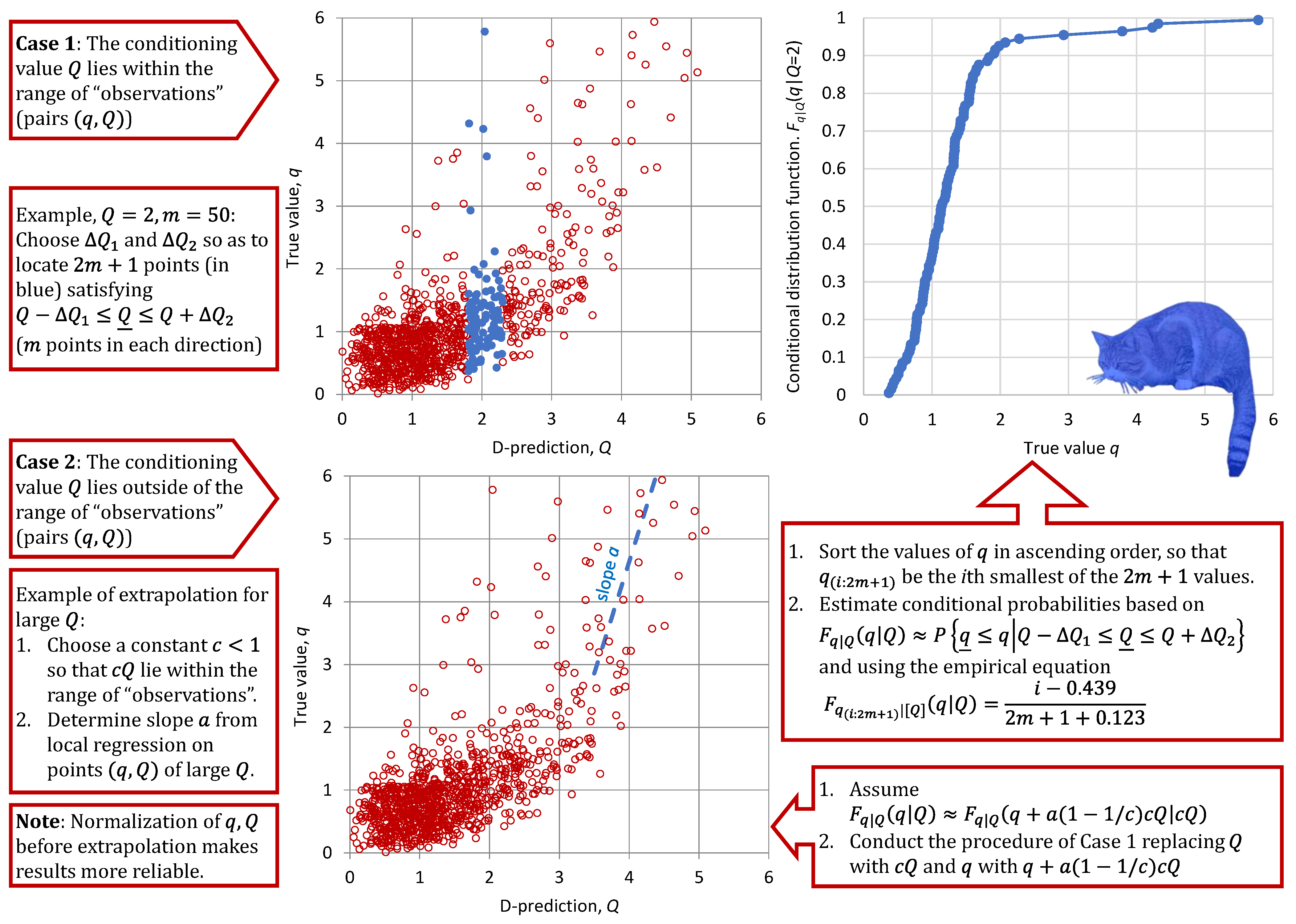
A schematic representation of the expanded Bluecat method is shown in
Figure 1.
3. Data
To apply Bluecat in combination with climate models, we chose as a case study area the entire territory of Italy. The reason we chose a big area, rather than a more hydrologically relevant unit, such as a specific catchment, is the known fact [
8,
10] that the performance of climate models improves by increasing the spatial scale. As case study variables of hydrological interest, we chose temperature and precipitation, both averaged in terms of area across the entire Italian territory.
As actual values of the processes of interest, we regarded those provided by the NCEP-NCAR Reanalysis 1 [
21], jointly produced by the National Centers for Environmental Prediction (NCEP) and the National Center for Atmospheric Research (NCAR). Its temporal coverage includes 4-times daily, daily and monthly values from 1948 to the present at a horizontal resolution of 1.88° (~210 km at the equator). It uses a state-of-the-art analysis/forecast system to perform data assimilation using observations and a numerical weather prediction model. The data assimilation and the model used are identical to the global system implemented operationally at NCEP, except in the horizontal resolution. A large subset of these data is available as daily and monthly averages (
https://www.esrl.noaa.gov/psd/cgi-bin/data/testdap/timeseries.pl; accessed on 25 February 2022). The data were retrieved from the climexp platform (
http://climexp.knmi.nl/, section: monthly reanalysis fields; accessed 25 on February 2022), using as a geographical mask that of Italy, readily provided by the platform. The time series are plotted in
Figure 2 (temperature) and
Figure 3 (precipitation) for their entire time period (1948–2021).
As a deterministic model, we used the mean of the output data of the Coupled Model Intercomparison Project (CMIP6), noting that nothing would change in the methodology if we chose any particular member of the ensemble instead of the mean. Among the scenarios provided, we use the Scenario Shared Socio-Economic Pathways 245 (SSP245). The model outputs also go back to the past, extending over the time period of 1850–2100. They have again been accessed through the climexp platform (option: Monthly CMIP6 scenario runs; Case: CMIP6 mean).
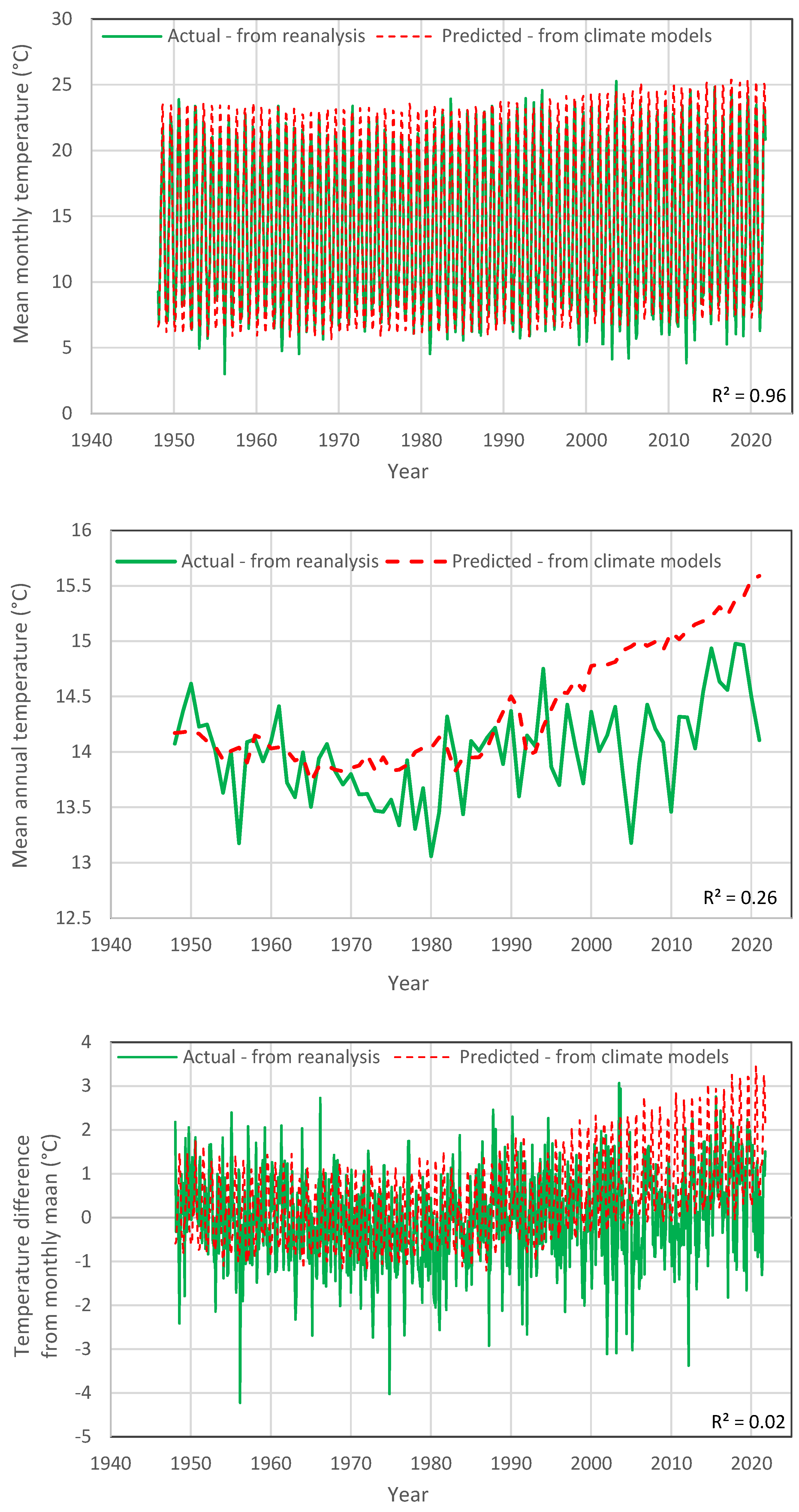
A comparison of the model outputs for temperature is shown in
Figure 2 for the common period of the datasets. In the upper panel, depicting the monthly data, it appears that the model agrees well with the actual temperature, with a very high coefficient of determination (
). This results from the fact that the model captures the annual periodicity, as materialized at the specific geographical location of Italy. If we average the process at the annual scale to eliminate the effect of periodicity (middle panel), then the agreement between the two datasets deteriorates (
). In particular, in recent years, the models predicted a considerable temperature increase, which however does not correspond to reality. The lower panel of the
Figure 2 also shows a comparison after reducing the effect of periodicity, but at the monthly scale; this was performed by subtracting the original values from the actual monthly means. Now, the D-model data show little correspondence to reality (
). Yet, the Bluecat method can be applied without problems, as it has been tested even with D-models that are irrelevant to reality. Specifically, it was demonstrated [
20] that, even in this case, Bluecat corrects the bias and properly evaluates uncertainty (which obviously is high, if the D-model is irrelevant to reality).
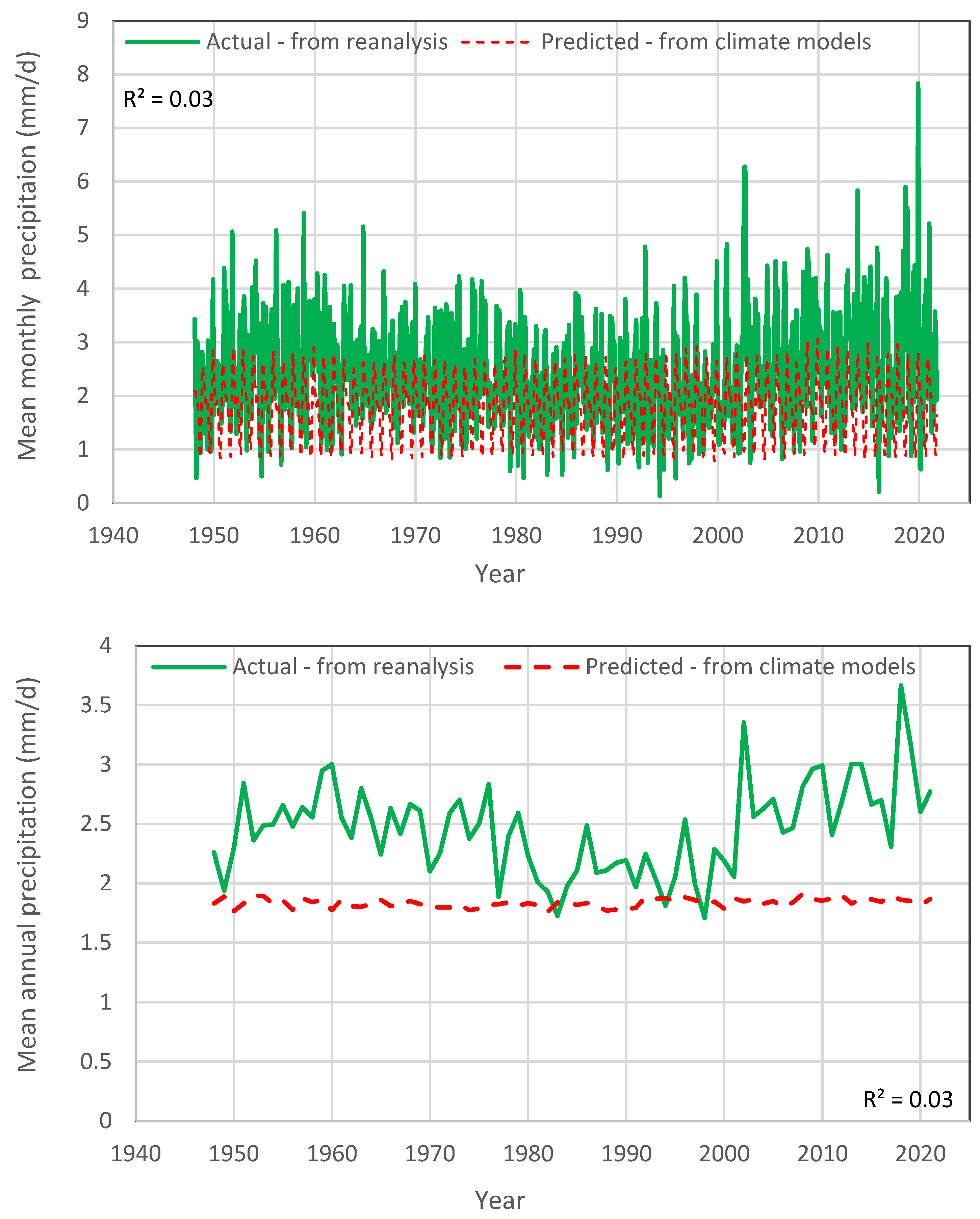
Likewise,
Figure 3 shows similar comparisons for precipitation. Now, the agreement of D-model with reality is poor both on the annual and the monthly scale (
). In particular, at the monthly scale, the D-model exhibits very low variability and, at the annual scale, it shows a horizontal line of stagnancy, which is different from what actually happens.
4. Results
For the temperature case, we applied Bluecat to the monthly differences from the means to avoid the construction of a more complex cyclostationary version of Bluecat, which would substantially reduce the available size of the dataset (e.g., in a monthly cyclostationary model, we would have 1/12 of the data for each month).
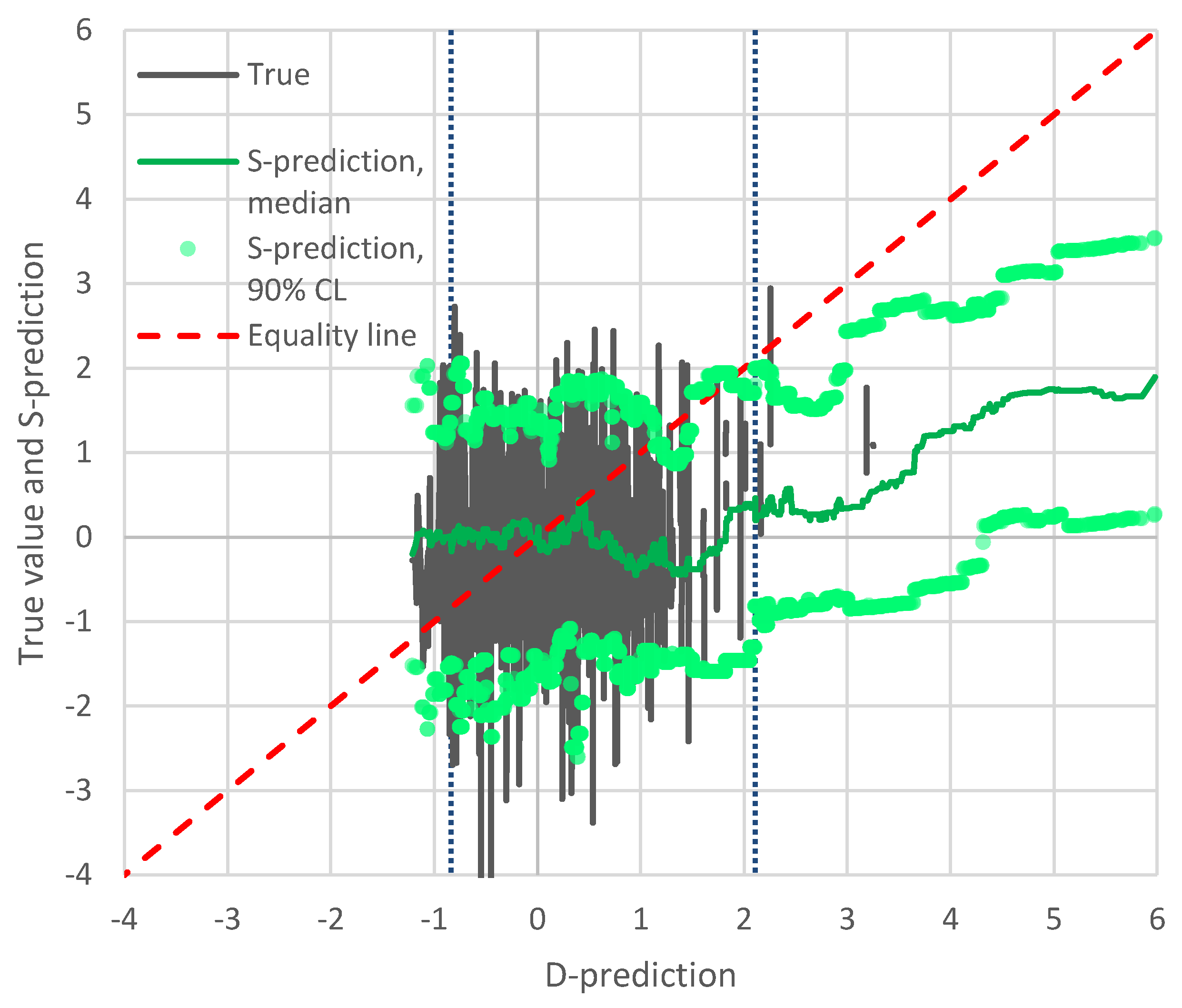
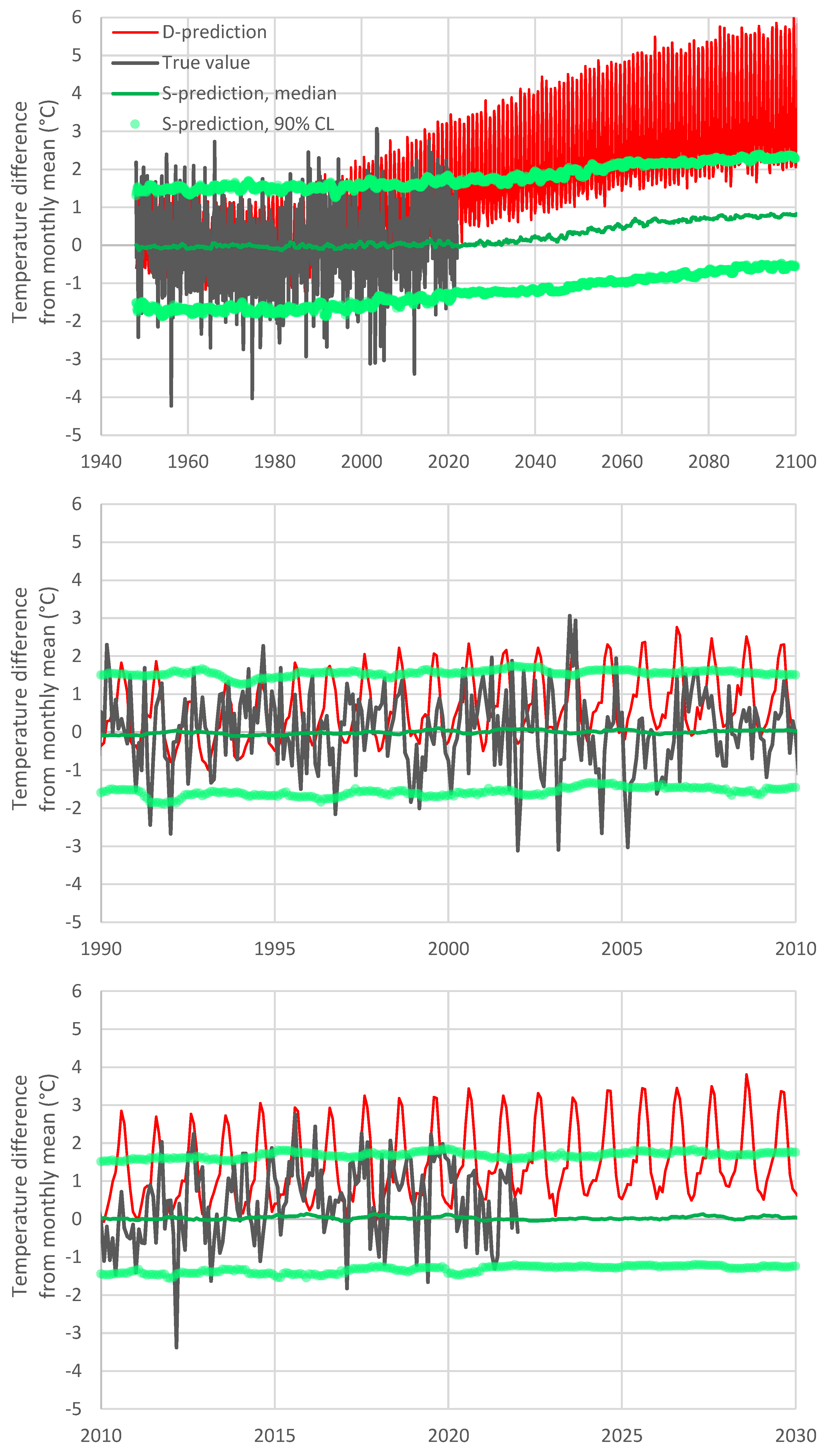
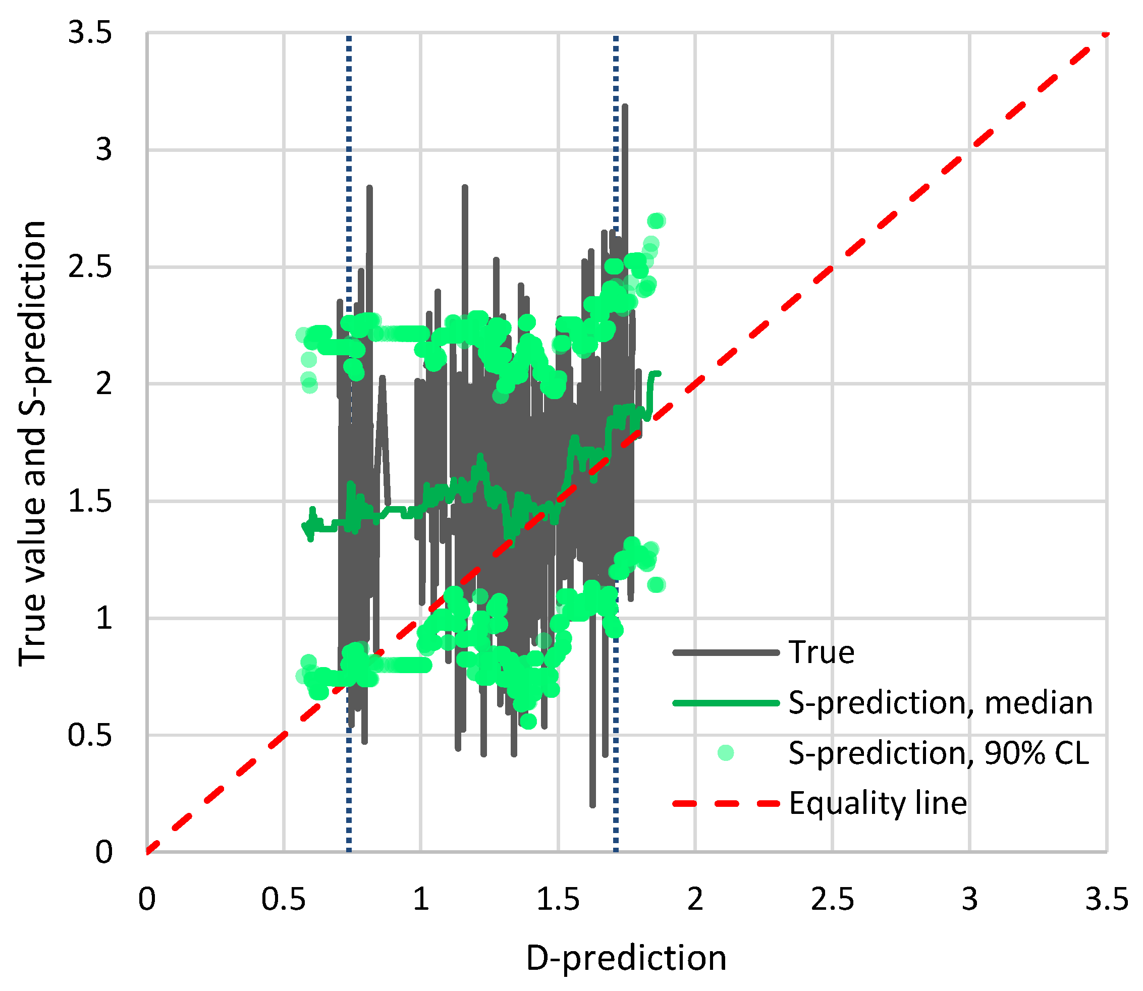
Figure 4 shows the results of the application of Bluecat to the temperature data. The graph depicts the true value and the S-prediction in terms of confidence limits vs. the D-prediction. The median S-prediction is also shown. The confidence limits are for a confidence coefficient of 90% (
for the low and high prediction, respectively). With reference to Equation (8), to estimate the value corresponding to a certain
, we solved the equation for
and rounded it to the nearest integer, and then calculated the
value as that corresponding to the
ith smallest value in the sample of
values. If the D-model was a good representation of reality, the median line would be close to the equality line and the confidence band would be narrow. In contrast, a totally irrelevant representation would result in a horizontal straight line with a wide confidence band. Here the situation is in between these two extreme cases. Yet, the performance of the D-model is not very good as the equality line is not enveloped by the confidence limit for high
Q-predictions.
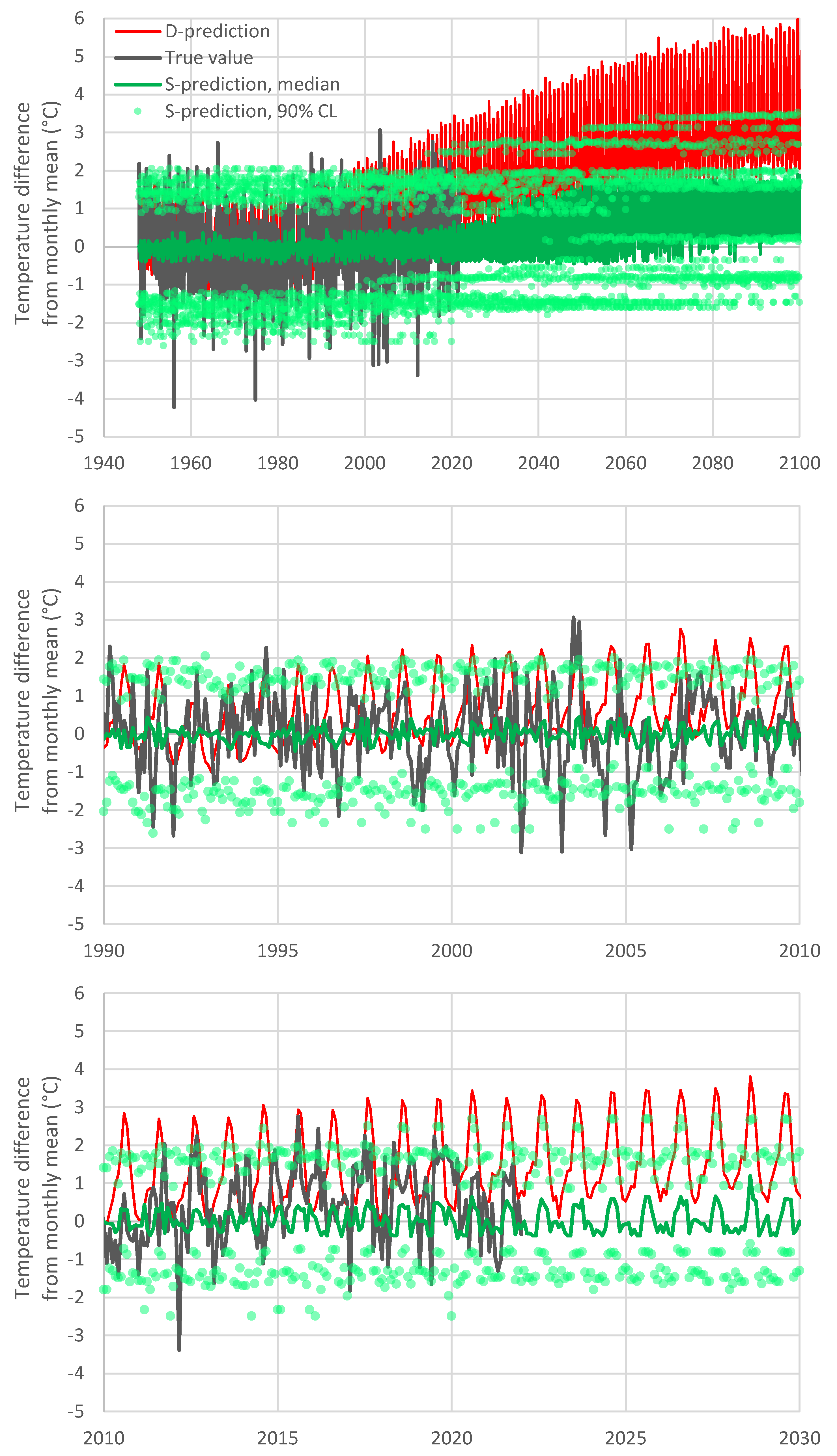
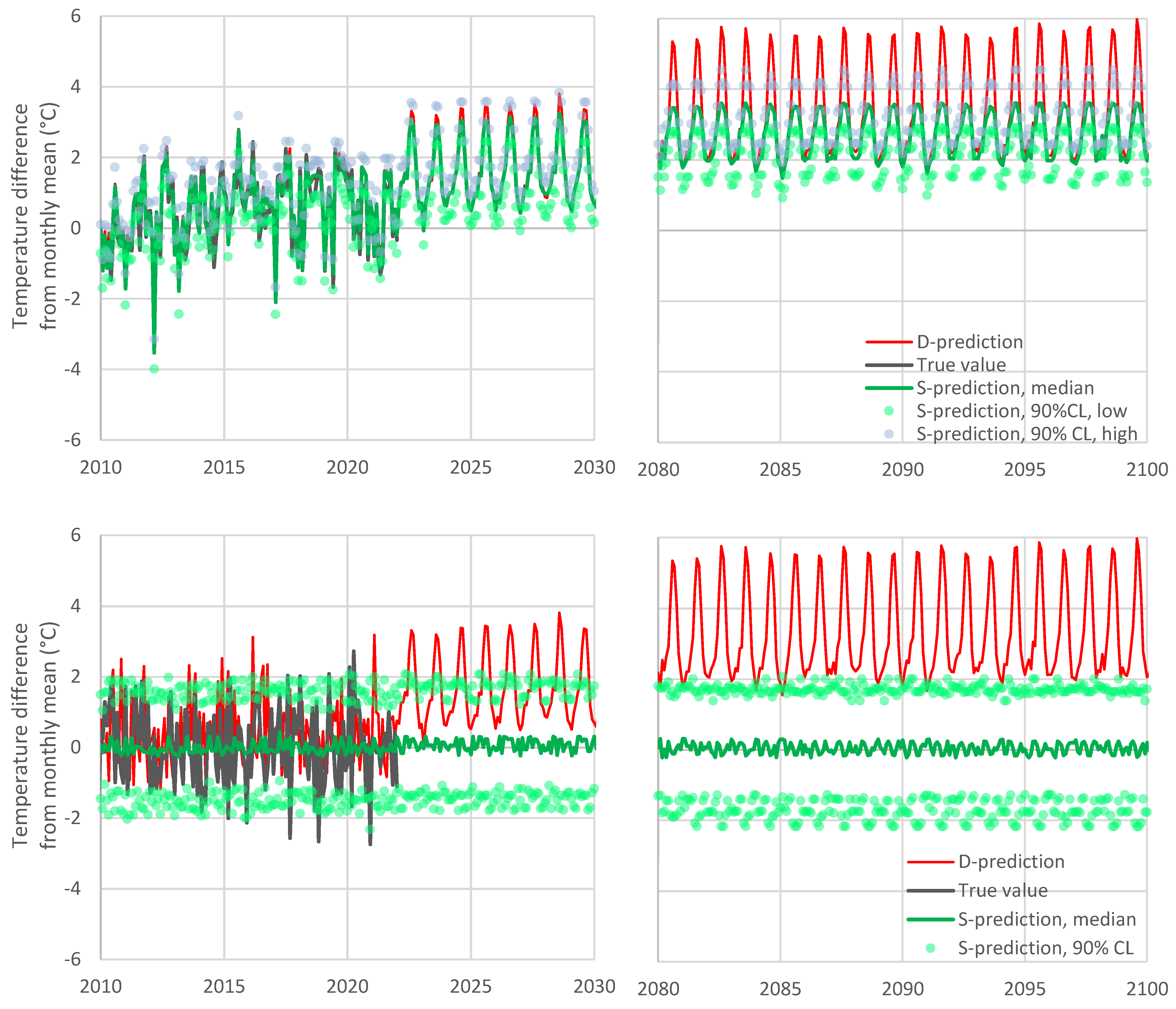
Therefore, as shown in
Figure 5, the evolution resulting from the S-model is quite different from that of the D-model. In the upper panel of the figure, it is seen that the increase rate of the future temperature according to the S-model is smaller than that predicted by the D-model. The reason why this happens becomes obvious in the lower panel of the figure, which focuses on recent years. Specifically, in the past ten years, the D-model has already departed from reality and, therefore, the departure increases in the future. This behaviour has recently been called
the hot model problem [
22], and, as seen in the rightmost area of the graph in
Figure 5, it is properly resolved by the S-model of Bluecat.
Another notable feature in
Figure 5 is the zig-zag shape of all predictions (D and S). This can easily be attributed to the excessive intensity of periodicity in the D-model. A simple remedy of this problem is shown in
Figure 6, where the monthly S-model values have been replaced by running averages with a 12-month time step.
One might potentially think to attribute the difference of the temperature increase rates of the D-model and S-model to the fact that the latter is stationary, while the former is not. However, this is not the case. The actual reason of the difference is the departure of the model from reality in the latest period. It is easy to demonstrate that Bluecat would behave well if the D-model had a better performance, which means that its stationary formulation is not a problem. This is graphically depicted in
Figure 7 (upper panel), where to make the D-model closer to reality, we replaced the D-model series with the weighted sum of true and D-model values with weights of 0.75 and 0.25, respectively. As seen in the figure, in this case, the S-model remains very close to the D-model even in the distant future (2100). While the entire methodology is based on stationarity, it captures the trendy shape of the D-model, provided that the latter is close to reality.
For the completeness of the investigation, the lower panel of
Figure 7 depicts a case where the D-model is totally irrelevant to reality. To implement this hypothetical case, we reordered the D-model series at random, so as to become uncorrelated to the true values. As expected, in this case, the S-model in effect disregards the D-model, producing horizontal lines of the future evolution, as expected for a stationary model. Even by disregarding the D-model, the S-model provides useful information, which is the stationary distribution function of the predictand.
For the precipitation case, in which the seasonal variation in Italy is not prominent, we applied Bluecat to the original monthly values. A second difference from the temperature case is that the rainfall distribution is far from normal and, therefore, we used the transformation of Equation (10) to normalize it. The resulting value of parameter
is 2 mm and the transformation, indeed, yielded a perfect fit to the Gaussian distribution.
Figure 8 shows the results of the application of Bluecat to the transformed precipitation data. The graph depicts the true value and the S-prediction in terms of confidence limits vs. the D-prediction. Notice that the ranges shown in both the horizontal and the vertical axes are intentionally identical. The fact that the true values cover the entire range, while the D-prediction values cover only a small portion of that range, is a result of the poor performance of the D-model. The median S-prediction is also shown, while the confidence limits are again for a confidence coefficient of 90% (
for the low and high prediction, respectively). It is seen in the figure that, for low precipitation values, the D-model is poor—the median S-model prediction is flat—but this improves for the highest predicted precipitation values, where the median line is close to the equality line. As already discussed (
Figure 3), the D-model underpredicts the actual variability of precipitation. Clearly, as shown in
Figure 8, this is corrected by Bluecat (compare the ranges of the plotted values on the horizontal and vertical axes).
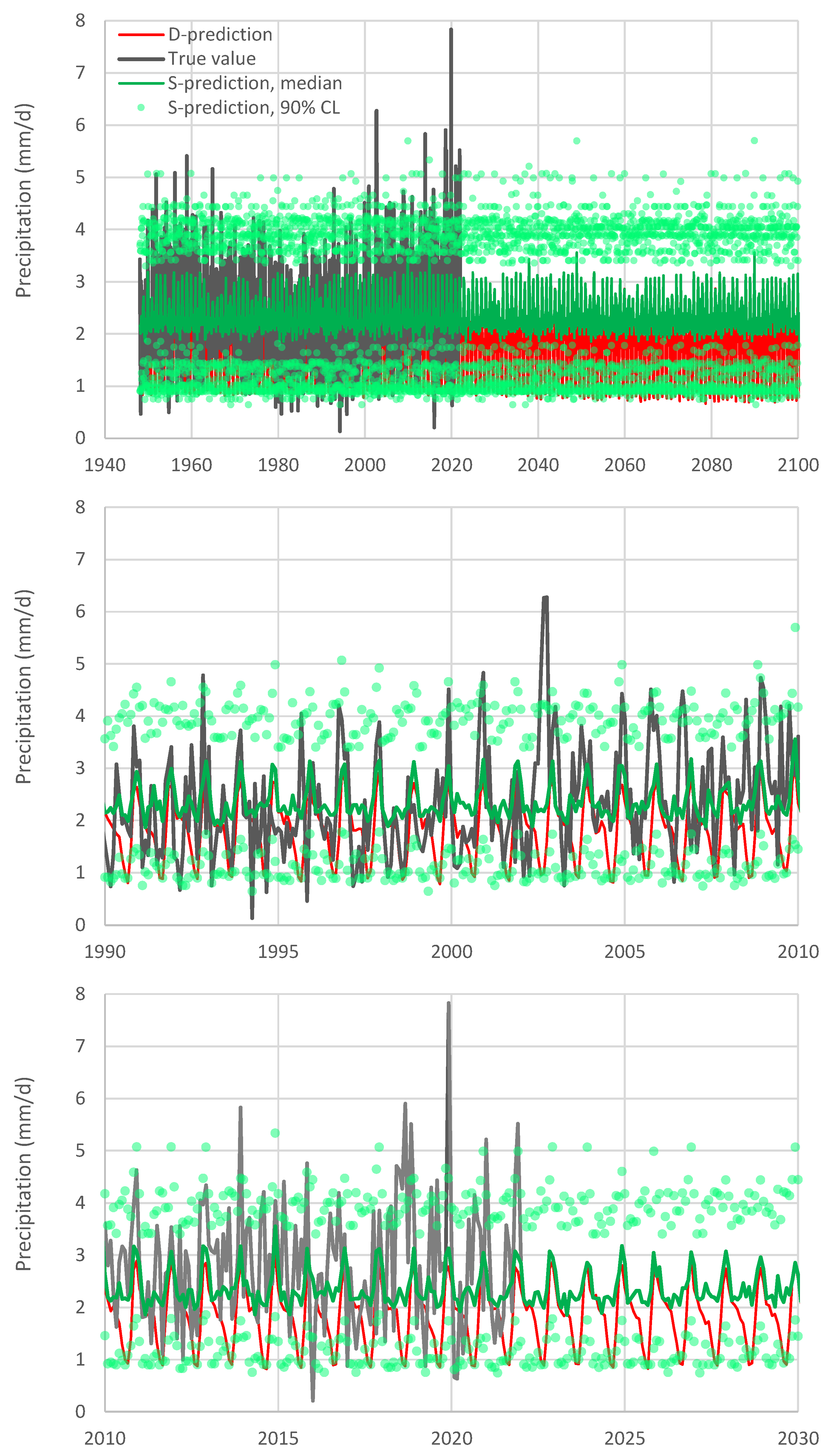
The evolution resulting from the S-model is shown in
Figure 9, after back-transforming to the natural rainfall vales. The substantial effect of the S-model, in this case, is that it widened the range of variability and corrected the bias. Generally, the D-model did not provide any substantial information and, even if we disregarded it, the results would not differ much. It must be further noted that, as the required range for extrapolation is not wide (see the vertical dotted lines in
Figure 8), even without using the normalizing transformation, the results are practically the same (not included in figures as the lines would be indistinguishable from those already shown).
5. Discussion and Conclusions
The Bluecat methodology, which was initially proposed as a hydrological modelling tool, appears to provide scientific means for incorporating climate predictions within hydrological modelling. Its theory is simple, transparent and easily understandable. Its key characteristic is the inference of the conditional distribution , where is the prediction of a deterministic model (D-model—in our case, the climate model) and is the true value of the predicted quantity. This conditional distribution is tantamount to a stochastic representation (S-model) of the true value. The advance from the D-model to the S-model offers two important functions:
Both the bias and the uncertainly characterization may differ for different ranges of , where the differences are automatically captured by the S-model by its construction. The conditional distribution is inferred from merely the data, i.e., concurrent values of model outputs and true values . The assumptions for inferring from the set of concurrent pairs (“observations”) of values ( are the following:
If the conditioning value lies within the range of “observations”, the conditional distribution is inferred using a subset of pairs with adjacent values. Namely, those pairs satisfying are chosen, where and are properly specified to form a sample of pairs that allows the empirical estimation of the conditional probabilities .
Otherwise, an extrapolation is made by the following method: A constant is chosen so that lie within the range of “observations” and the above method be applicable by replacing or with . Then, the conditional distribution is estimated by enrolling the relationship , where is a parameter representing a regression slope between and . This parameter is locally determined for the high or low values of , depending on the direction of the extrapolation.
The application of the expanded Bluecat method is also very simple as it does not require any sophisticated computational means. All these characteristics make Bluecat an ideal tool for enhancing collaboration of scientists with practitioners and decision makers.
Traditionally, the task of combining climate models within hydrology is termed “downscaling”, as hydrological models require finer scales than those resolved in climate models. An additional (and most important) job of the downscaling techniques is to adjust climate model outputs (such procedures are sometimes termed “bias correction” of statistics), making them consistent with local measurements. In this, downscaling techniques resemble the proposed method. However, our method has substantial differences from downscaling techniques, including the following:
The scales of the application of the Bluecat’s S-model are not necessarily different from that of the climate D-model. They could be precisely the same, as in the present application to Italy. In this respect, Bluecat makes the D-model consistent with reality irrespective of spatial scale. Apparently, the case where the scales are different (e.g., smaller area of the S-model with respect to that corresponding to the D-model) is also served by the proposed methodology, without any change with respect to what is described above.
The Bluecat methodology considers both the time sequence and the amplitude of the D-model and actual series. It does not make a lumped fitting on the entire set of past data to find unique parametric relationships to be applied to the adaptation of the future values (as usually conducted in downscaling techniques). Nor does it regard the future values as correct ones that only need downscaling. Rather, it treats past and future values produced by the D-model in the same manner—as representing a model and not the truth.
In addition to modifying a D-model series, correcting it for bias, Bluecat advances it to a stochastic representation, thus characterizing the uncertainty that is illustrated in this paper in terms of confidence bands.
In fact, the stochastic representation is much more than drawing confidence bands. Its real power emerges in stochastic simulation, by which a system can be tested in a Monte Carlo approach so that the uncertainty of the process of actual interest (e.g., river stage or discharge, reservoir outflow and inundated area) is eventually evaluated. This has not been included in the scope of this paper, but is currently under research, whose results will be reported in the future.
Some features of the Bluecat framework have not been included in this study in order to keep it as simple as possible. These features include a more sophisticated calibration approach, relying on a split-sample technique with different calibration and validation periods, which was not necessary in this paper. Additionally, they include the concept of knowable moments (K-moments [
19]) for a more robust estimation of empirical distribution quantiles, while it is also useful for the construction of a simulation framework.


