Article

Towards Informed Water Resources Planning and Management

1
Research Centre for Water and Environment, Department of Civil Engineering, University of Siegen, Paul-Bonatz Strasse 9-11, 57068 Siegen, Germany
2
The World Bank, 1818 H Street Northwest, Washington, DC 20433, USA
3
Italian Hydrological Society, Piazza Porta San Donato, 40126 Bologna, Italy
*
Author to whom correspondence should be addressed.
Hydrology 2022, 9(8), 136; https://doi.org/10.3390/hydrology9080136
Submission received: 29 June 2022 / Revised: 26 July 2022 / Accepted: 26 July 2022 / Published: 30 July 2022
(This article belongs to the Collection Feature Papers of Hydrology)

Abstract

:
In Water Resources Planning and Management, decision makers, although unsure of future outcomes, must take the most reliable and assuring decisions. Deterministic and probabilistic prediction techniques, combined with optimization tools, have been widely used to meet the objective of improving planning as well as management. Bayesian decision approaches are available to link probabilistic predictions to optimized decision schemes, but scientists are not fully able to express themselves in a language familiar to decision makers, who fear basing their decisions on “uncertain” forecasts in the vain belief that deterministic forecasts are more informative and reliable. This situation is even worse in the case of climate change projections, which bring additional degrees of uncertainty into the picture. Therefore, a need emerges to create a common approach and means of communication between scientists, who deal with optimization tools, probabilistic predictions and long-term projections, and operational decision makers, who must be facilitated in understanding, accepting, and acknowledging the benefits arising from operational water resources management based on probabilistic predictions and projections. Our aim here was to formulate the terms of the problem and the rationale for explaining and involving decision makers with the final objective of using probabilistic predictions/projections in their decision-making processes.

1. Introduction

The availability of water resources varies temporally and spatially, mainly depending on three factors: precipitation, evapotranspiration, and infiltration into the soil. Precipitation is the main water supply in a watershed, while evapotranspiration, depending on various factors, including solar radiation, wind, and vegetation, is the main cause of water loss. Infiltration into the soil and groundwater recharge is not a loss (in the strict sense, except for surface water) as it can accumulate in aquifers for use at different times and/or places. The temporal non-uniformity of surface water resources often requires regulating their availability by means of storage systems, such as reservoirs. For example, in many cases, abundant fall–winter flows correspond to modest spring–summer regimes. In these cases, reservoirs of adequate volume are constructed to hold the flows during the period when they are abundant and to release them during the drier seasons when the resource is perhaps needed for irrigation or other uses.
In some cases, on a larger scale, a reservoir must not only allow the regularization of interannual flow fluctuations, but also of multiannual fluctuations to compensate for droughts that are prolonged over several years. The typical case of such type of management is that of the Aswan reservoir, which was designed to regulate the Nile flows for up to ten years, as the droughts in this system can be very persistent.
In the planning phase, the management rules can be of “empirical” type, namely, defined either on the basis of empirical rules by the experience of managers or by simple deterministic models. Alternatively, management can be of the “optimized” rational deterministic or stochastic type, controlled by maximizing expected profits (or minimizing expected losses) over a long period of time by means of stochastic optimization. In many cases, reservoirs are managed based on a set of operational rules established according to the current reservoir levels and the prediction of future inputs on one or more-time scales. If for small tanks the adjustment is carried out in ten-day time steps, in general, monthly steps are used for large volumes. However, as already stated, most reservoirs are still regulated on an empirical basis, according to the experience acquired by the managers in maintaining very high safety margins, and centered on the false impression that, in this way, the operational rules remain simple and easy to implement. However, it has been shown that even optimized management rules, and in particular stochastic rules, not only lead to higher profits, but can also be carried over to simple indications provided by a decision-support system to the reservoir manager.
Optimized deterministic regulation is derived on the basis of the expected value of the forecast, but has all the disadvantages mentioned in the previous section because it implicitly assumes that the predicted value coincides with the value that will occur, which is usually improbable, and does not assess the consequences of ignoring other possibilities. On the contrary, the optimized probabilistic regulation, as a function of a decision to be taken based on probabilistic forecasts, considers the whole range of possible future events by weighing them by the predictive probability density to evaluate their expected consequences and chooses the decision that minimizes expected losses and/or maximizes expected benefits taking into consideration all possible future occurrences [1,2]. Optimized probabilistic regulation is more complex in the derivation phase but, in the operational phase, it leads to simple rules comparable to empirical ones, which can be easily integrated into a decision support system.
In addition, because it is possible to re-evaluate the predictive distributions at each time step, stochastic probabilistic regulation can adapt to situations of short-term non-stationarities, like, for instance, the arrival of a flood wave or long-term non-stationarities, such as those due to climate change.
The benefits deriving from this type of regulation are very high. An example relating to the regulation of Lake Nasser, the Aswan Reservoir [3], as shown in attached Figure 1, demonstrates that the benefits of an optimized adaptive stochastic regulation can lead to more than 65% benefits over those produced by a rule of thumb.

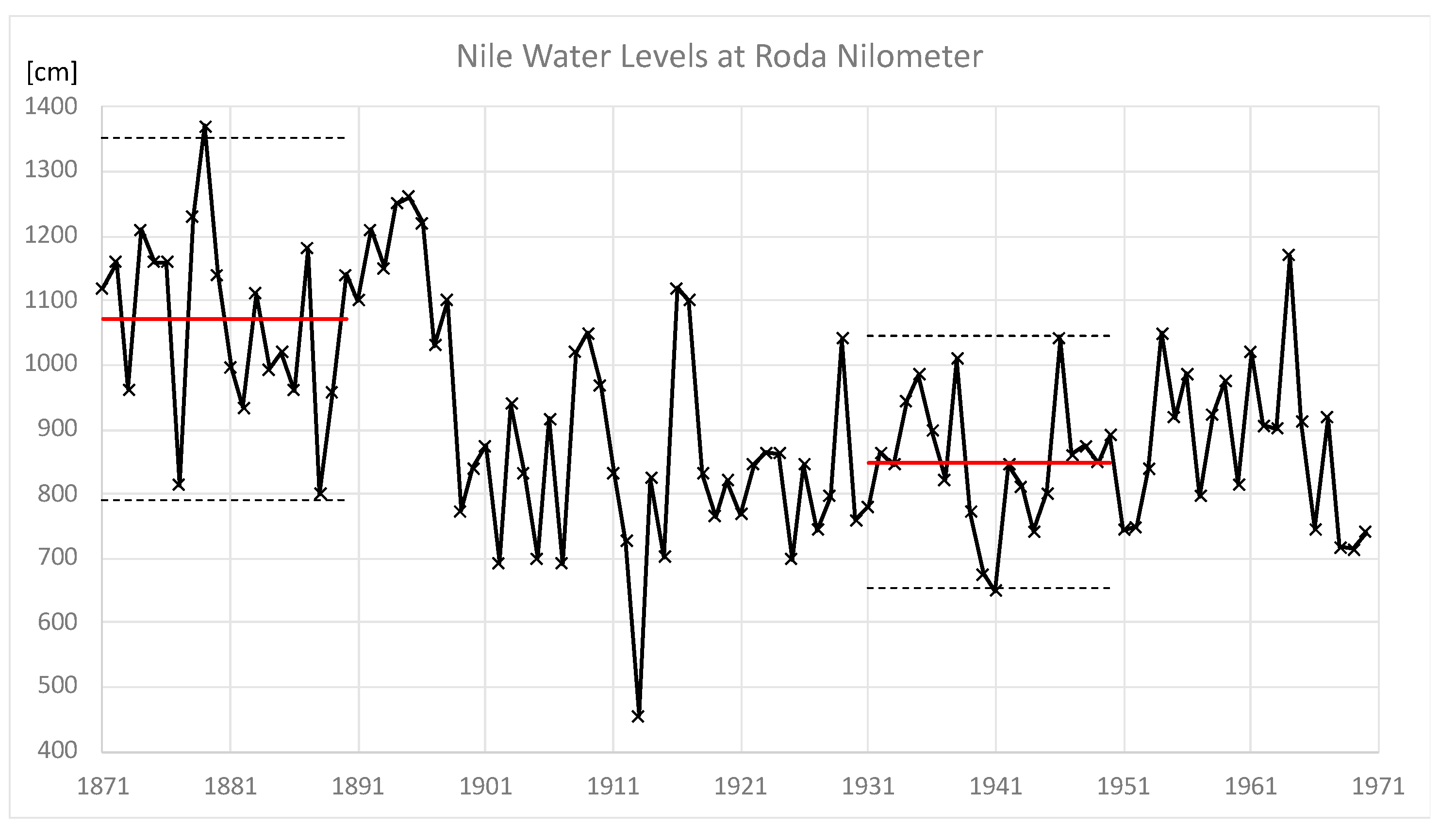
1.1. Management under Stationary Conditions

In a reservoir, the optimized management rules based on stochastic forecasting are generally derived using Dynamic Stochastic Programming (PDS) which acknowledges the distribution of the predictive probability from one time step to the next (generally from month to month) to maximize the expected value of profits or minimize the expected value of both immediate and future losses, depending on any reservoir release assumption. To do this, it is necessary to first estimate the probability distribution of future reservoir inflows as a function of the present value. This procedure, under the assumption of a stationary-type regime, is performed by constructing a stochastic predictive model, usually a first-order autoregressive model, otherwise known as a Markov chain, by which it is possible to derive the probability distribution at a future time step, conditional on the present step. This model is estimated from all the historical data available under the very restrictive assumption of stationarity (i.e., the probability distributions do not vary over time) and ergodicity (whereby is possible to estimate the probability distribution at an instant from the data observed at different time steps).
Thus, knowing the state of the system, such as the volume stored in the reservoir at the present time and the inflow of the current month, it is possible to estimate for each release hypothesis the expected value of future profits or losses. The optimal decision would, therefore, be the one which minimizes this expected value.
For many years of the last century, this approach was indeed the best choice. However, since the 1980s, there has been a sudden change of meteorological regime in many countries, including the Mediterranean region, which has brought down the validity of the stationarity hypothesis, thus reducing the effectiveness of the management rules established thus far. Indeed, adaptive stochastic regulation requires the correct evaluation not only of the expected future value of water inputs, but also of their entire predictive probability distribution, which, in the case of climate change, will be very different from that estimated for the historical period.

1.2. Management under Non-Stationary Conditions

If the stochastic optimization approach of management rules remains valid, what varies in a non-stationary context is the conditional probability distribution, which encounters the following two challenges: (i) it can no longer be derived from historical data, except under certain restrictive assumptions, and, more importantly, (ii) it cannot be used as is for the future precisely because of climate change, the evolution of which is unknown at present.
Regarding the historical period, in order to estimate the probability distributions in a non-stationary regime, if the evolution is not extremely fast, as under climate change conditions, it is possible to identify periods that are not too long (say 20–30 years) in which it is still possible to apply the hypothesis of a weak stationarity (at least limited to the first two or three moments of the probability distribution) and of ergodicity, to proceed by analogy as in the stationarity regime (Figure 2).
However, the problem of extrapolating these probability distributions to the future remains, since it is no longer possible to establish them for future periods by assuming stationarity over long periods of time. Due to loss of stationarity, it is no longer possible to extrapolate outright the estimated probability distributions defined over the historical period. The only sensible way to proceed is, therefore, that linked to the use of one or multiple General Circulation Models (GCMs), which make it possible to extend the chronological series in the future by considering strong non-linearities and the chaotic nature of the global atmospheric system. Unfortunately, these sets of models are incorrectly used to estimate future predictive probability distributions without conditioning them to observations [4]. Only by conditioning the forecasts of one, or better of several, of these models on the basis of actual observations, can we correctly estimate the predictive probability distributions, which acknowledge both the non-stationarity, due to climate change, and the link to the past or current climate. It is finally this probability distribution, conditioned on models and reality [4] that we propose to use in the stochastic optimization phase in adjusting reservoir management rules.

2. Basic Concepts

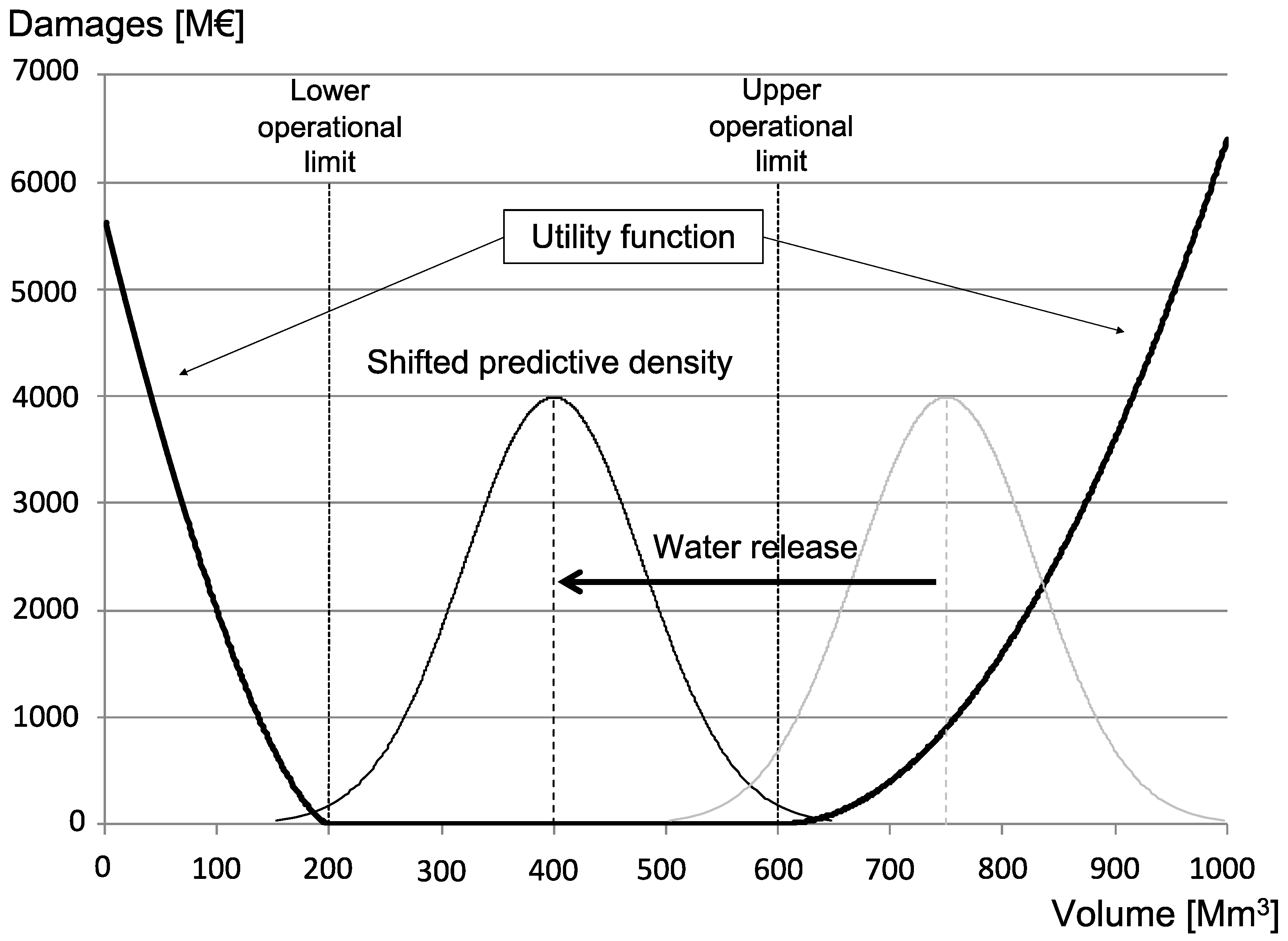
2.1. Decisions under Uncertainty

Traditionally, most water resources management rules and decisions are based on deterministic criteria, such as exceeding a threshold by an observed parameter. For example, reservoir releases are increased if the stored volume exceeds an upper limit volume or reduced if the stored volume drops below a lower limit volume. All this is fine, if the quantity, which triggers the decision, is observed and thus known, except for small measurement errors which are insignificant for decision-making and which make it possible to assume a “perfect knowledge” of the quantity itself. An example can be the issuance of river flood alerts based on progressive level thresholds that trigger the different phases of attention, guard, and alert. Measurement errors of a few centimeters are in fact irrelevant for subsequent decisions and the levels can be considered perfectly known. However, this approach is only useful for large rivers, where the rate of rise of the levels is low enough to allow for the implementation of actions planned and programmed in each of the risk mitigation phases. On the other hand, when dealing with small rivers, where the rate of level rise is high and the time left to overflow short, the decision-making method based on real-time measurements cannot be adopted, because, when a threshold is exceeded, it is often too late for a correct implementation of mitigating actions. In these cases, instead of measurements, predictions of future levels are compared against the trigger thresholds of the different phases. Unfortunately, the uncertainty associated with predictions is significantly higher than the one of measurements, resulting in a significant decrease in efficiency and robustness of subsequent decisions. Likewise, when it is necessary to decide how much water to release from a reservoir in the upcoming 10–30 days, without exact knowledge of how much the natural inflow will be, it is necessary to base the decision on an estimate or, even better, on a forecast of what the state of the reservoir will be at the end of the time horizon of interest. This involves basing decisions on predictions and not on recorded reservoir levels by considering the uncertainty of the future state of the system. Unlike measurements, forecasts provide much more imprecise knowledge about future reservoir levels, with errors (the difference between what is predicted and what will happen) that by far exceed those from measurements and, in particular, to an extent that is non-negligible for decision-making purposes. Therefore, we are in a situation of having imperfect knowledge of the future, and hence the pre-set release levels alone do not provide all sufficient information to correctly make the most optimal decision.
The predicted quantities, such as, for instance, future reservoir levels, represent only expected values, but do not provide additional information, such as how they are distributed and, in particular, an estimate of the spread of the future levels around the forecast values. In other words, the probability of occurrence of values lower or higher than the expected ones is high. On the contrary, probabilistic predictions aim at fully describing, through a probability distribution or an ensemble, the lack of knowledge on the future outcomes, which is the essential information to assess the expected benefits or losses descending from any taken decision.
To better understand this concept, consider the case of deciding whether to release a volume of water from a reservoir in the face of a forecasted flood inflow. If we base our decisions exclusively on a “deterministic” prediction, then, if not explicitly, we still implicitly assume that the future volume will always be “exactly” the same as expected, with the obvious result that each time the future volume substantially differs from the expected value, we inexorably make major decision errors.
Figure 3 shows the case of a reservoir of set storage capacity. If the volume does not exceed a predetermined maximum level, the losses caused by the overspill of the reservoir are zero, otherwise they increase following a second-order power law, as expressed by the cost function. By relying on a forecast, if we assume that the expected value of the volume provided by the forecast is a deterministic quantity, the expected loss estimate L o s s e s ( E { V } ) = 0 will be zero, as shown in the left pane (a) in Figure 3, because the predicted value of the volume does not exceed reservoir capacity. However, the forecast expresses an expected value, meaning that “on average” the future value will be equal to the expected value, but it could also depart from that value with extremely high or low levels being less likely. Therefore, to complete the information, it is necessary to predict not only the expected value, but also the entire density function, which allows one to assess the consequences of events that lie besides the mean, by weighting them with their occurrence probability. This concept is explained in Figure 3. The left pane (a) shows the calculation of spillage losses resulting from the expected value of the reservoir levels (deterministic forecast); here the losses are zero because the single predicted deterministic value triggers no spillage. On the contrary, the right pane (b) shows the expected value of the forecast as well as the entire predictive probability distribution. The probability of excess volumes leading to reservoir spillage (blue-shaded area) is non-zero.
To prevent the exclusion of all those excess reservoir volumes that could potentially induce losses, one needs to estimate the probability-weighted losses instead of those corresponding to an expected value of the reservoir level as in the left pane. In the latter case our evaluation does not acknowledge the uncertainty of the forecast, leading to a no-spillage prediction, that is often proved wrong. To correctly decide whether to release water ahead of an event, we need to estimate the “expected losses”, defined as integral between the spill gate level volume and infinity of the product losses (the function indicated by a black curve in Figure 3) times the probability of occurrence of the corresponding volume (the function indicated in blue):
E { L o s s e s } = V m a x L o s s e s ( V )   P r o b ( V )   d V > 0
The expected value of the losses will differ significantly from zero, as visible in the left pane (a) of Figure 3, because one cannot exclude the occurrence of water levels that are sufficiently high to cause downstream losses. It is obvious that the expected value of losses E { L o s s e s } is something other than the value of losses L o s s e s ( E { V } ) calculated using the expected value of the reservoir volume. While the latter is zero, the same losses estimated by acknowledging the uncertainty that values larger than the reservoir capacity may occur is non-zero. They may even be substantially larger than zero, i.e., E { L o s s e s } > > L o s s e s ( E { V } ) = 0 .
This is a general result in the presence of uncertainty, when the relation between the decision variable (in this case the losses) and the predicted value is of nonlinear or discontinuous type, as in the case of the reservoir, due to the presence of a threshold V m a x and the activation of the nonlinear loss-volume relation for V > V m a x . Deciding not to release water ahead of an event, given that a supposedly deterministic forecast suggests zero-loss, leads inevitably to weak and often wrong decisions, because many alternative values with non-negligible probability of occurrence are a priori excluded. To correctly estimate the expected value of the profits (or losses) resulting from decisions when we are not sure about the future, we need to estimate and provide the entire predictive probability distribution and not just the mean value; then, we need to use the assessed predictive distribution to calculate the expected value of profits or losses. What mostly occurs in practice in the context of probabilistic forecasting is to rather estimate the predictive distribution only to provide an indication of the uncertainty by means of classical confidence limits and rarely to derive stochastically optimized management rules. In practice, the information provided by the entire predicted probability distribution, which can add valuable information if properly used in a decision-making scheme, is replaced by using two values only, the maximum and the minimum. These two extreme values are supposedly representative of the dispersion of the population which have the unwanted collateral effect of fomenting a negative perception among decision makers towards considering uncertainty.
This can be shown through the example shown in Figure 4. The left pane (a) provides information on the average daily temperature across different months in the form of probability densities which, in the event of damage exceeding predetermined thresholds, make it possible to calculate their expected value. On the right pane (b), however, the same information is provided as an average value ±   1 standard deviation. Here the only information that can be obtained is that the average is uncertain, and that the uncertainty varies across months. However, if the predictive distribution is not Gaussian, we have no way of calculating the expected values of the quantities that interest us for informed decision-making. This approach, instead of increasing the confidence of decision makers, generates a sense of indeterminacy and unwarranted additional uncertainty.
The reason why we speak of unjustified lack of confidence is related to the fact that in reality the uncertainty is reduced (say “marginalized”) by the calculation of the expected value of the profits (or losses), which aims at reducing, as far as possible, the effects of chance by integrating the product of profits (or losses) by their corresponding probability of occurrence. To give an idea of this point, one needs to bear in mind that the estimate of the mean value of a sample is less uncertain by a factor 1 / n ,   than the individual observations of the original sample, with n the number of observations. In case of a sample of observations, we start from the definition of the expected value:
E { x } = 0 x   f ( x )   d x
Then, noting that the probability distribution is no longer continuous, but discrete, we go from the integral to the summation and marginalize the uncertainty by assuming that each observation has the same probability of occurrence p ( x i ) = 1 / n , to obtain the classical estimator of the expected value (the mean):
E { x } = i = 1 n x i   p ( x i ) = 1 n i = 1 n x i  
For reasons given above, this value is inherently less uncertain than individual observations. Essentially by taking the expectation over the observations sample we have marginalized the original uncertainty. If we deal with normally distributed variables the mean and the variance fully qualify the probability distribution, but apart from yearly average values most natural variables, and in particular precipitation and discharge, show clear skewed and more complex distributions when sampled at seasonal, monthly, or shorter time intervals. Hence the need to marginalize uncertainty by using the information provided by the predictive density requires the entire probability distribution, not only the mean and at most two confidence limits, to be considered if there are to be robust decisions.

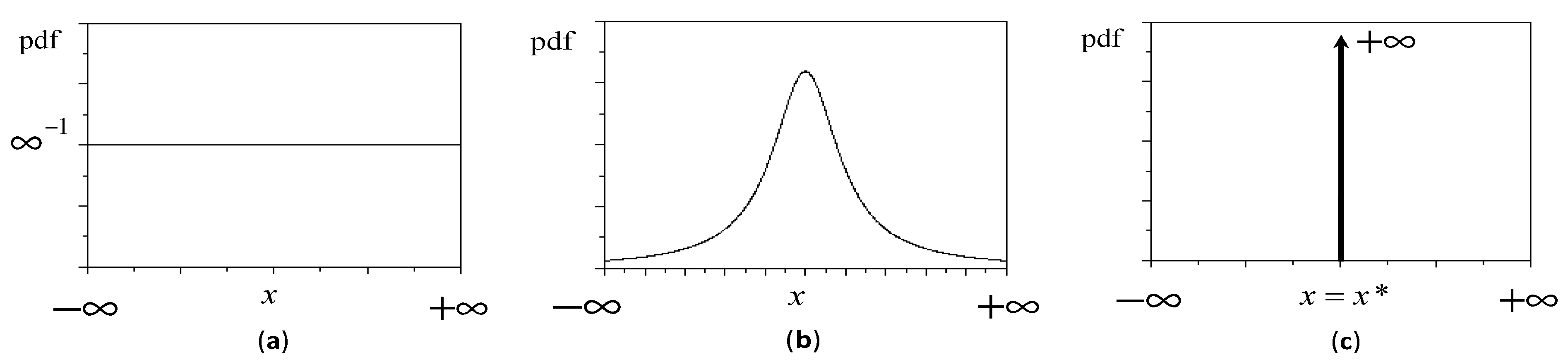
2.2. The Mathematical Representation of Knowledge

Various forms of mathematical approaches exist for the quantification of information about knowledge and its opposite, uncertainty, due to lack of knowledge. Different ways of characterizing knowledge have been proposed, ranging from fuzzy sets [5] to grey sets [6] and are widely used when it comes to non-commensurable quantities. However, when we want to express knowledge of measurable quantities, such as discharge and water volumes, it is useful to define knowledge according to statistical probability density functions.
Total absence of knowledge (i.e., full ignorance) is represented by a uniform probability density of infinitesimal value over the entire field of existence (in the most general case between negative infinity and positive infinity), which indicates that any value has the same probability of being correct, but without knowing the right one [7]. An example of a uniform distribution is given by the left pane in Figure 5. Perfect knowledge (i.e., the complete absence of ignorance) is represented by a mathematical operator of infinite magnitude and infinitesimal thickness over the exact value called the Dirac delta [8] (Dirac, 1958). It represents the fact that all information is concentrated in this value and is shown in the right pane in Figure 5. Each intermediate case of imperfect knowledge (or partial ignorance) is represented by a classical probability density function, usually bell-shaped (middle pane in Figure 5). This curve indicates that we know approximately the correct value, which we expect to coincide with the mean, but that we are unsure about because the exact value could be higher or lower than the mean, and is, in other words, dispersed around the mean. The probability density function describes how the probability mass is distributed across the variable range, over which we acknowledge uncertainty, knowing that the actual value is located somewhere within.
To better grasp this concept, suppose we need to measure the width of a table in a dimly lit room with a measuring instrument (e.g., a tape measure) that is not very readable, so that it is easy to get a wrong reading. If we repeat the readings after measuring the same length, we will find that the measured values will probably differ from each other and that the frequency of observation is distributed according to the bell-shaped Gaussian probability density function, which becomes the most complete representation of our knowledge. The mean of the observations will also be uncertain, although its uncertainty decreases as the number of observations increases, until it collapses into a Dirac delta function on a single value, when an infinite number of observations is reached. This is equivalent to saying that we are in a situation of perfect knowledge. This value will obviously only be exact if our measuring instrument is unaffected by systematic errors, and would, otherwise, be biased.
All this shows that in most situations we possess imperfect knowledge. This means that to be able to provide correct information, this knowledge must be described by a probability distribution and not by a single value, such as the population mean.

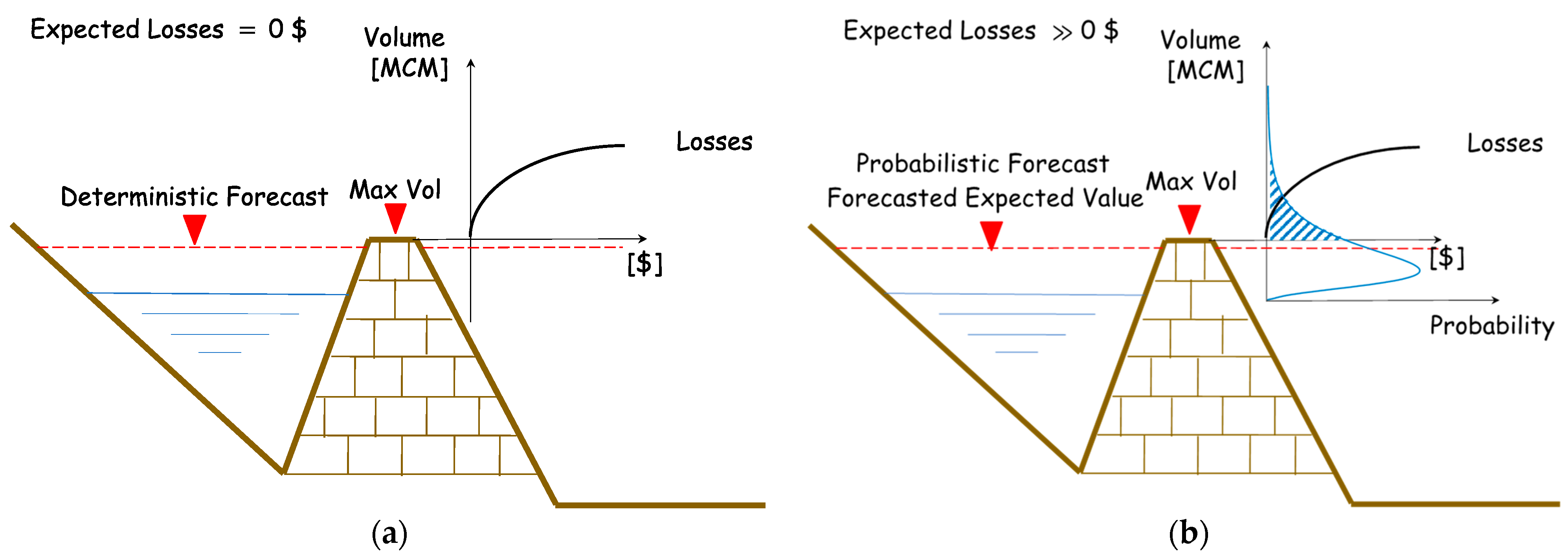
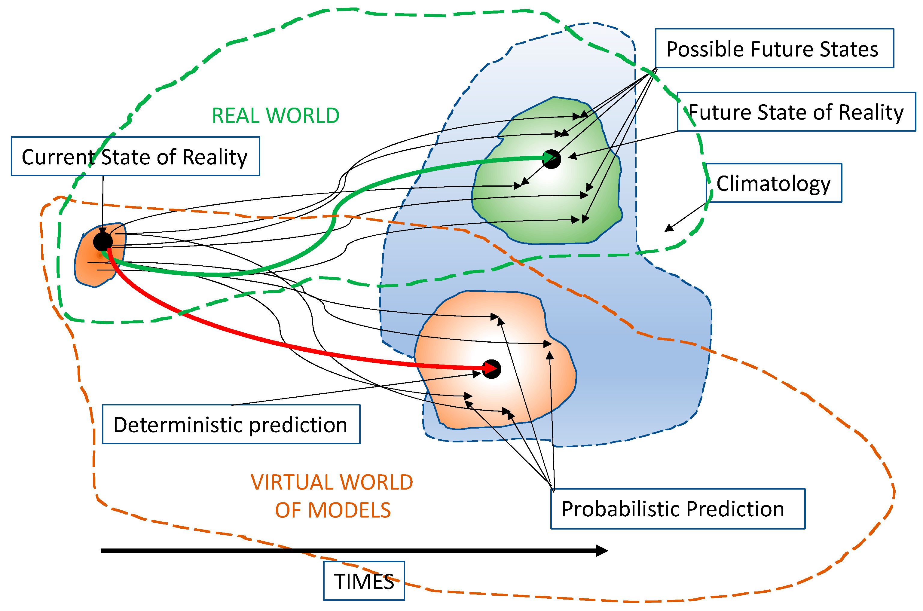
2.3. Deterministic versus Probabilistic Forecasts

To better understand the concept of “forecasting” in the context of planning and managing water resources, especially the risks associated with droughts and floods, it is necessary to consider “forecasting” as the only “measure” (or rather “pseudo-measure”) available of the future state of a system. In other words, what is of interest is not the forecast itself, given by one or multiple predictive models, but the actual state in which the quantity of interest (e.g., the volume of the reservoir) will be found at the end of the time horizon, as the only information, in the form of a “pseudo-measure”, albeit uncertain, provided by a single or multiple models.
Indeed, it is uncertain that the evolution of forecasting models in the future will correctly mimic the evolution of the real system, because of their implicit simplified and approximate representation of system complexities. This concept is visualized in Figure 6, where we show how the actual current state, such as the state of the atmosphere or a water resources system, evolves over time to reach a future state following a given trajectory (green line). The figure also shows a shaded area, which indicates other potential points that are “physically” reachable by the natural (real) system starting from the current state. However, when making a decision, we not only do not know the value, which will be reached by the state variable, but we also do not have a description of all the points towards which the real system can potentially evolve (green shaded zone).
To get an idea of what may occur, we adopt one or multiple models describing the evolution of the physical system, knowing that the future states reached by the models will most likely not coincide with the true ones and that the possible future states of the models (orange shaded zone) will hardly coincide with potential real future states (green shaded zone). From this, two aspects emerge. The first concerns the fact that only the actual future states, and not the future states predicted by the models, will provide information about the uncertainty of the future system state. The second is that a deterministic forecast will neither allow the uncertainty of the future states of the models to be described nor, more importantly, that of the real future states, which is essential when estimating potential benefits or losses.
The benefits or damages are produced by the actual and not by the expected triggering variables. Therefore, estimating the expected value of the consequences of future states requires involving the probability distribution of the actual future states, and not the uncertainty of the states generated by the models. We, therefore, need to build a kind of “translation dictionary” which converts forecast uncertainty estimated by models (orange shaded zone) into the corresponding forecast uncertainty of real future states (green shaded zone). This “translation dictionary” is called “conditioning”. In other words, we must find the probability distribution of real future states depending (conditional) on the knowledge of the probability distribution provided by the models.

3. Probabilistic Predictions

3.1. Short Term Probabilistic Forecasts

Short term forecasts are essential for the day-to-day operation of reservoirs as well as for flood risk management. The forecasting horizon varies from a few hours to several days depending on the time required to assess the effects of decisions to be taken based on the forecasts and the time needed to implement them.
Accuracy of forecasts decays with the length of the forecasting horizon which is limited by the characteristic concentration time of the upstream catchment. Accurate short-term deterministic forecasts can be provided on large rivers using flood routing hydraulic models with upstream flow or water level measurements when the travel time of the flood waves is long enough. Longer forecasting horizons may require a cascade of catchment rainfall-runoff and flood routing models with a corresponding loss of accuracy. When the required forecasting horizon becomes larger, one also requires the use of quantitative precipitation forecasts to extend predictions beyond the concentration time of the catchment, which adds additional degrees of uncertainty.
Sometimes data-driven models, such as artificial neural networks, are also used for short term forecasting with apparently reasonably good results. Nonetheless, there are two reasons that make deterministic models preferable. First, while deterministic models, particularly the ones based on detailed topographic description and mass and energy balance equations, such as the flood routing models, can extend their validity beyond their calibration range, data-driven models often become unreliable. The second reason relates to the fact that when dealing with flood risk attenuation measures, it is common practice to compare the effects of alternative interventions, which may modify the topology or, more generally, the internal structure of the systems under control, such as allowing waters to invade water detention areas or activate a bypass, etc. This is relatively simple to simulate using physically based models, but rather impossible to do if using data-driven models without a time-consuming re-calibration process, which is not possible under the stress of the incoming events.
As discussed in Section 2, deterministic forecasts, which may be considered as expected values, are not sufficient to take informed decisions, a process requiring the assessment and use of the full predictive density. Accordingly, several uncertainty processors were developed in the past decades to describe the predictive distribution function, namely the probability distribution function of the future “real” occurrence conditional on a deterministic forecast, which is now taken not as the real future outcome but rather as its uncertain “pseudo-measurement”. Several uncertainty processors have been developed from the Model Output Statistics approach [9,10], to the Bayesian Model Averaging due to Raftery [11], the Bayesian Forecasting System developed by Krzysztofowicz [12], the Quantile Regression approach due to Koenker [13], and, more recently, the Model Conditional Processor [14].
Most of the above-mentioned approaches deliver the predictive distribution conditional on the “deterministic” prediction, namely the expected forecasted value produced by the predictive model is used, which can be of any type: physically based, conceptual or data driven.
The new generation of uncertainty processors also allows the combining several predictive models of different types [15], as well as accounting for time dependence in predictions (e.g., [16,17,18,19]).

3.2. Medium Term Probabilistic Forecasts

Medium term forecasts of reservoir inflow can be obtained by different approaches, depending on the size of the river basin, data availability and the predictability of the flood wave propagation in the flow channel. The use of the following are possible options: (i) autoregressive models; (ii) rainfall-runoff models, that are forced by long-term weather forecasts; (iii) seasonal forecasts.
Auto-regressive (AR) models [20] establish a linear stochastic relationship between a stochastic process variable and p time-lagged copies of itself, hence the name “auto-regression”. The number of lagged series used in the regression determines the order p of the autoregressive model used. The chosen time-lag is process-dependent and varies for river flow processes between several hours to days or months. The number of predictors at previous time steps that are used to describe the dependency with the predictand are the “order” of the autoregressive model. The AR model can also include the dependency on additional process variables, so-called exogenous variables, leading to ARX models. In the case of flow forecasts on large rivers with slow flood propagation, an ARX model, which uses up-stream stations as exogenous input, works well, because the flood propagation is usually highly predictable. Such data-driven model approaches are operationally used all over the world to forecast the rise of flood waves in slow-varying systems. For instance, the annual flood wave of the lower river Niger caused by seasonal precipitation in the far-distant headwater basins of equatorial West Africa, and flood waters traveling multiple thousands of kilometers on very mild slopes, can be predicted with high accuracy based on pure ARX modeling. The same can be said for the Nile or other large-scale river systems. A major advantage of autoregressive flow modeling is the data-driven approach, which demands only modest computational resources as no solution of physical governing equations.
Other types of regression-based models, like the moving average (MA), have been proposed for flow modeling. MA models base the forecast on a linear combination of lagged forecasting residuals that are added to the long-term observed average with a white noise component. In combination with an AR model, one obtains the so-called ARMA models that can be extended to include exogenous variables (ARMAX). Nevertheless, the ARMAX models are not well suited for flow forecasting applications, as the predictive skill of the MA component collapses in the absence of recent observations and auto-regressive models with exogenous variables (ARX) are then preferred.
If flow observations are too scarce to set up data-driven models, flow forecasts can be obtained with the use of hydrological models that simulate the rainfall-runoff process in the river basin. These parameterized models need to be calibrated over a historical period with observed precipitation and discharge data. In prognostic operation, hydrological models are forced by medium- and extended-term numerical weather predictions (NWP) that are produced by national meteorological services and are available at different temporal scales. Medium-range forecasts cover typical forecasting horizons up to 15 days, extended-range ones up to 6 weeks. Medium- and extended-term forecasts provide predictions of how the average atmospheric ocean and land surface conditions over areas and periods of time are likely to deviate from the average and provide the atmospheric states as means over several days. Smaller-scale temporal resolutions of the variables are also available or can alternatively be obtained by temporal disaggregation of the mean product. The choice of the right forecasting time horizon for medium- to extended-range hydrological flow forecasts is primarily dependent on basin size and concentration time. For small to medium-sized river basins, medium-range precipitation and temperature forecasts may be sufficient for flow forecasting. Continental-sized basins, on the other hand, can have concentration times with lengths of multiple weeks to months, thus requiring extended-range weather predictions or long-range forecasts addressed below.
Seasonal prediction scales are covered by long-range forecasts with typical time horizons between 6 to 7 months. For instance, the rather novel SEAS5 ensemble product for operational seasonal climate forecasting by the European Centre for Medium-Range Weather Forecasts (ECMWF), which replaces the older ECMWF System 4 with a large international community of users, constitutes a new attractive development at the seasonal scale. The research in [21] carried out verifications of SEAS in forecasting precipitation and daily minimum/maximum temperature for the Australian continent, based on 36 years of re-forecast data, pointing out the predictive capabilities. While the benefits of these types of products for small watersheds are limited, due to the high degree of spatial uncertainty, they provide added value in long-term predictions for extensive systems, especially when future liquid precipitation, as well as snow cover area and depth, need to be estimated with sufficient lead time. Such information is especially valuable for the management of large irrigation schemes or for estimating hydropower energy production potential for the upcoming season.
Potential users of short- to long-term weather forecasts must consider that NWP model output is inherently uncertain. In combination with the parameter and initial conditions uncertainty of the hydrological model, this leads to flow predictions that are affected by uncertainty to different degrees, manifesting itself in the spread of the predictive distribution. Various approaches exist to sharpen [22] the predictive distribution. Data assimilation with the aid of Kalman filtering (e.g., [23]) can be used to update model states and, hence, sharpen the posterior distribution of predicted flow.

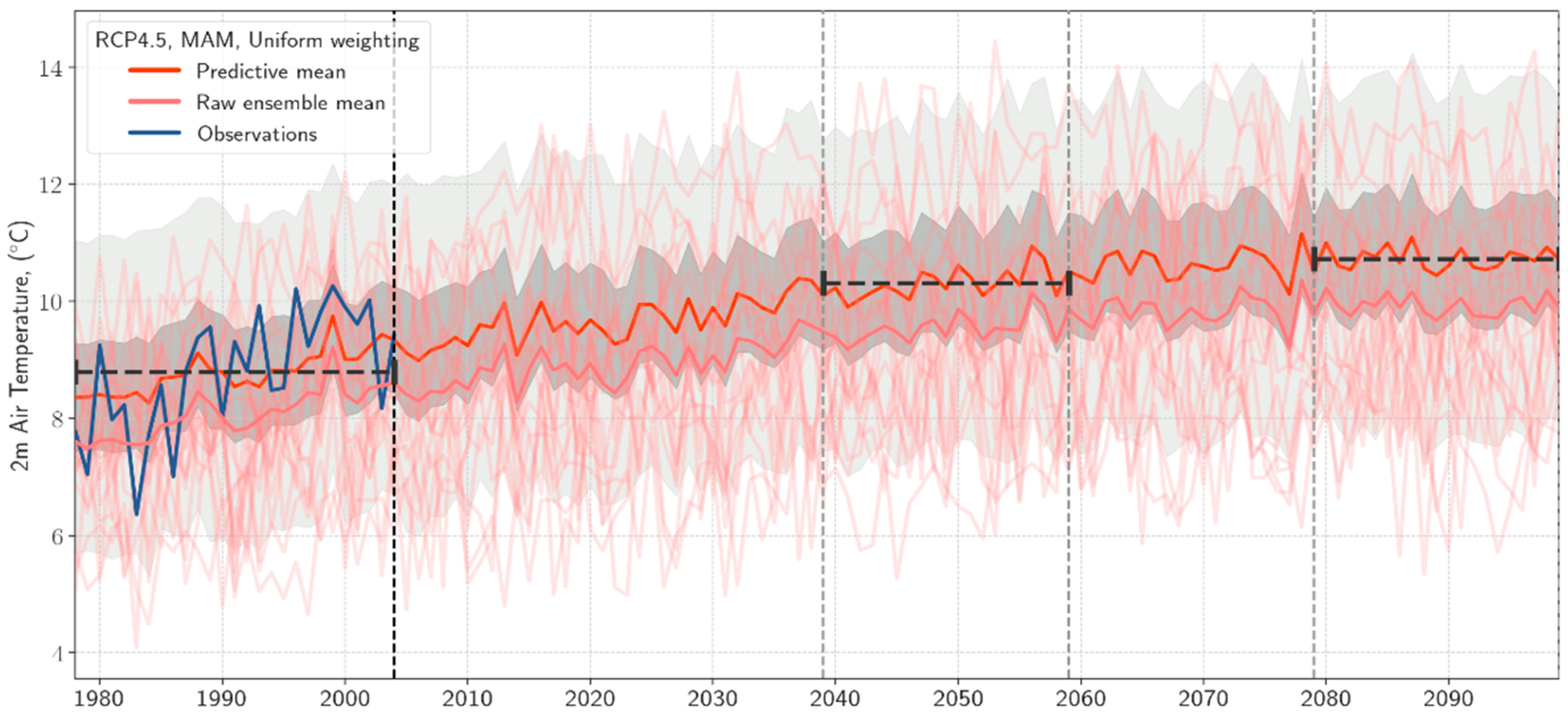
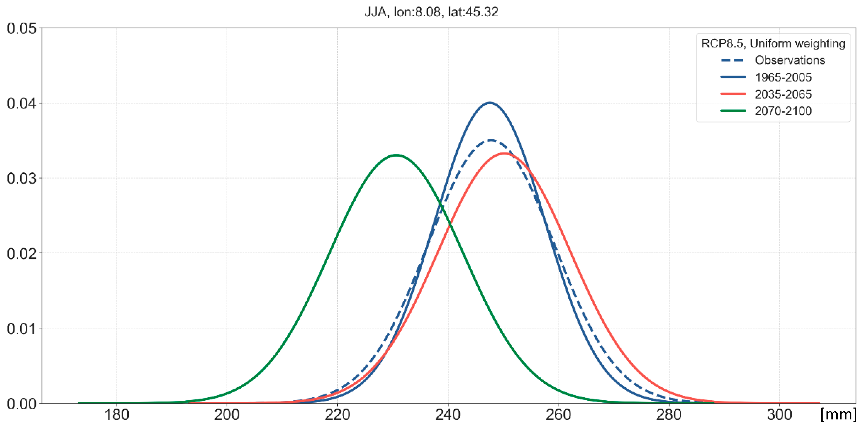
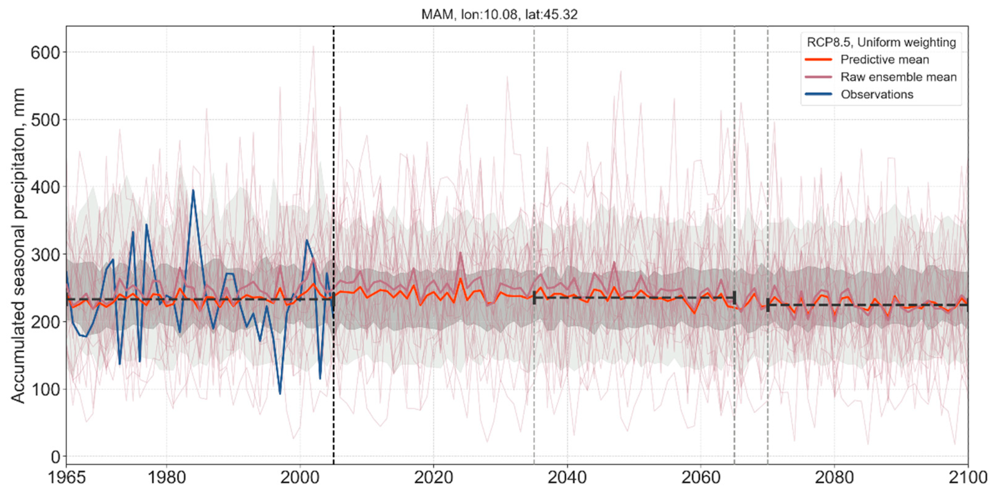
3.3. Long-Term Probabilistic Climate Projections

For predictions at very long climatic time scales, the only option is to rely on the projections of Earth-system models, which simulate, as realistically as possible, the interaction of atmosphere, land, ocean and sea-ice processes. The solutions of the physical governing equations are sensitive to model uncertainties, owing to the fact that complex non-linear thermodynamic processes are simulated in an approximate way, and that the equations are resolved on a finite grid. The time integration of Earth-system models driven by different Representative Concentration Pathways (RCPs) leads to an ensemble of projections that can be used to estimate the response of the Earth’s climate to radiative forcing [24]. We note here that the term ‘projection’ is used instead of ‘prediction’, because future integrations that extend beyond a few years are mainly driven by the particular radiative forcing scenario adopted, rather than by the initial conditions, as is the case with medium range to seasonal weather predictions. Several multi-model ensemble simulations of future climate have been performed as part of the Climate Model Inter-comparison Project (CMIP), which, to date, includes multiple executive phases [25,26,27,28]. One also needs to bear in mind that the principal difference between handling climate projections versus classical short- and medium-range forecasts is that presently available climate projections may be capable of preserving the statistical properties of the simulated Earth-system variables, but not their observed auto- and cross-correlation structures [29] as in medium-range to seasonal weather predictions. Hence, only projections at annual seasonal, or at least monthly, scale are of interest for decision-making processes, while daily-scale fluctuations are near meaningless in a climatic context.
Figure 7 shows post-processed ensemble projections for RCP4.5 seasonal temperature projection, March-April-May, averaged over the river Po basin, Italy. The left-hand side window is the 1979–2005 control period used for data calibration against observations, whereas in the middle and on the right the 2040–2060 and 2080–2100 prognostic windows are visible. The two horizontal dashed lines represent the mean of observations and the predictive means for the two prognostic windows. Figure 8 visualizes the post-processed ensemble projections of precipitation for the pessimistic RCP 8.5 scenario in a CMIP5 1° × 1° reference cell. While temperature in the river Po valley is clearly increasing, precipitation remains overly stable during the 21st century. Figure 9 displays the probability densities of the predictive means and observations for the control period and the two prognostic windows. It is using these predictive densities that one can estimate the expected losses as per Equation (1).

4. Attracting the Interest of Decision Makers

One of the primary objectives of hydrologists involved in prediction is to attract the interest of decision makers to the explained probabilistic aspects. The main reason is that in the case of hydrological predictions, it is only rarely the case that predictions expressed in the form of predictive densities have been fully understood, accepted and introduced in the decision-making process. In most cases, they have been merely used to attach a measure of reliability to a “deterministic” forecast based on the mean (mean forecast, mean of an ensemble of forecasts, etc.).
The reasons for this mostly descend from the following general aspects:
  • inappropriate definition of predictive uncertainty;
  • misunderstanding of the meaning of predictive uncertainty and of its role in decision-making;
  • unclear role and use of epistemic uncertainty (such as parameter uncertainty), which is often confused with predictive uncertainty;
  • incorrect use of ensembles in the assessment of predictive uncertainty;
  • misunderstanding of the mechanism and of the advantages for using predictive uncertainty in the Bayesian decision-making process.
All these points have been discussed at length in the hydro-meteorological literature [3,30,31,32,33,34,35,36], but the most important point on the list, relevant to the Bayesian decision approaches [37], remains number five, because if decision makers could fully grasp the benefits, in terms of increased decision reliability in conjunction with reduction of expected damages and increase of expected benefits, they would unavoidably turn in favor of probabilistic forecasting.
To clarify point number 5, Figure 10 shows a generic example where environmental losses occur if the volume in a reservoir falls below the lower operational limit of 200 Mm3 while environmental, social, and economic losses rapidly increase when the volume overtops the upper operational limit of 600 Mm3. The utility function in Figure 10, expressed in monetary terms (€), is generally set up in cooperation with the decision maker to reflect his or her subjective views and risk propensity.
A forecast of the future stored volume is available at the end of the forecasting horizon in the form of a Gaussian predictive probability density with mean 750 Mm3 and standard deviation 80 Mm3. As can be visually noticed from Figure 10, the integral of the product between the predictive density, represented by the thin, grey, bell-shaped curve, and the utility function gives a large expected loss of about 1 million . By releasing water from the reservoir, although there would be loss of precious water volume, expected losses could be dramatically reduced. Releasing water is equivalent to shifting downwards the predictive density by the released quantity. The situation of Figure 10 after releasing 350 Mm3 shows that the updated predictive density, represented by the black solid line bell shaped curve, is shifted downwards and the expected losses ( ~ 30   ) become practically null.
Prior to clarification with the decision maker, and with regards to the other four and more technical points of the above list, we strongly recommend setting up a simulation environment capable of retrospectively comparing the results of many successive informed decisions obtained through the probabilistic Bayesian scheme against the results obtained using rigid deterministic operating rules commonly used by decision makers. In this way the decision makers would immediately become aware of the advantages and disadvantages of the proposed innovative approach of taking operational decisions by acknowledging the importance of the information introduced through a correct description of the predicted uncertainty.

5. Conclusions

Operational water management is a conservative business, which relies on simple and well-proven rules, whose immediate and long-term consequences must be easily comprehendible for stakeholders and political decision makers. Nevertheless, such rigid rules very often lead to suboptimal water use and poor management of the resource. Over-exploitation of a multi-purpose reservoir leading to lack of water during critical periods is a classic example.
Growing global stresses concerning water resources, partly due to climatic changes, partly due to increasing water demand, make poor management practices increasingly unaffordable and support the concept that more flexible water resources management approaches need to be adopted, in which the use of an increasingly scarce and variable resource is optimized, and bankable benefits reached.
Such an approach must abandon the rigid decision schemes, based on deterministic system predictions, independent of the time horizon, and instead acknowledge the randomness of the forecasted natural flow processes, known as aleatoric uncertainty. The latter outweighs by far the epistemic uncertainty attributable to intrinsic limitations and process parameterizations of numerical models used in forecasting.
Certainly, state variables such as precipitation, temperature and surface water flow that are retrospectively predicted by climate and hydrological models, need to be conditioned on observations first, hence removing biases and adjusting variances, to become useable with more confidence as predictors for the yet to be observed future state variables. The so-obtained predictions are uncertain and characterized by predictive probability distributions. In conjunction with a cost utility function, these predictive distributions enable a probability-weighted expected estimate of management consequences to be traded-off against actual costs, thus supporting objective decision-making.
Without communicating and integrating uncertain weather, climate, and surface water information routinely into the decision processes, objective and cost-effective water resource management decisions will remain an elusive endeavor. This brings us to the need to develop strategies aimed at approaching decision makers by guiding them to recognize the benefits descending from informed decisions. We need to also support them in understanding the indispensability of the proposed approaches with increased water scarcity and climate change impacts.

Author Contributions

Conceptualization, E.T., P.R. and A.T; writing—original draft preparation, P.R. and E.T.; writing—review and editing, E.T., P.R. and A.T. All authors have read and agreed to the published version of the manuscript.

Funding

This research was partly funded by Deutsche Forschungsgemeinschaft (DFG), grant number RE3848/4.

Data Availability Statement

Not Applicable.

Acknowledgments

We would like to acknowledge all organizations that have provided openly available data to complete this research, in particular the CMIP5 group of institutes for the climate projections.

Conflicts of Interest

The authors declare no conflict of interest.

References

  1. Schwanenberg, D.; Fan, F.M.; Naumann, S.; Kuwajima, J.I.; Montero, R.A.; dos Reis, A.A. Short-Term Reservoir Optimization for Flood Mitigation under Meteorological and Hydrological Forecast Uncertainty. Water Resour. Manag. 2015, 29, 1635–1651. [Google Scholar] [CrossRef] [Green Version]
  2. Todini, E. Paradigmatic changes required in water resources management to benefit from probabilistic forecasts. Water Secur. 2018, 3, 9–17. [Google Scholar] [CrossRef]
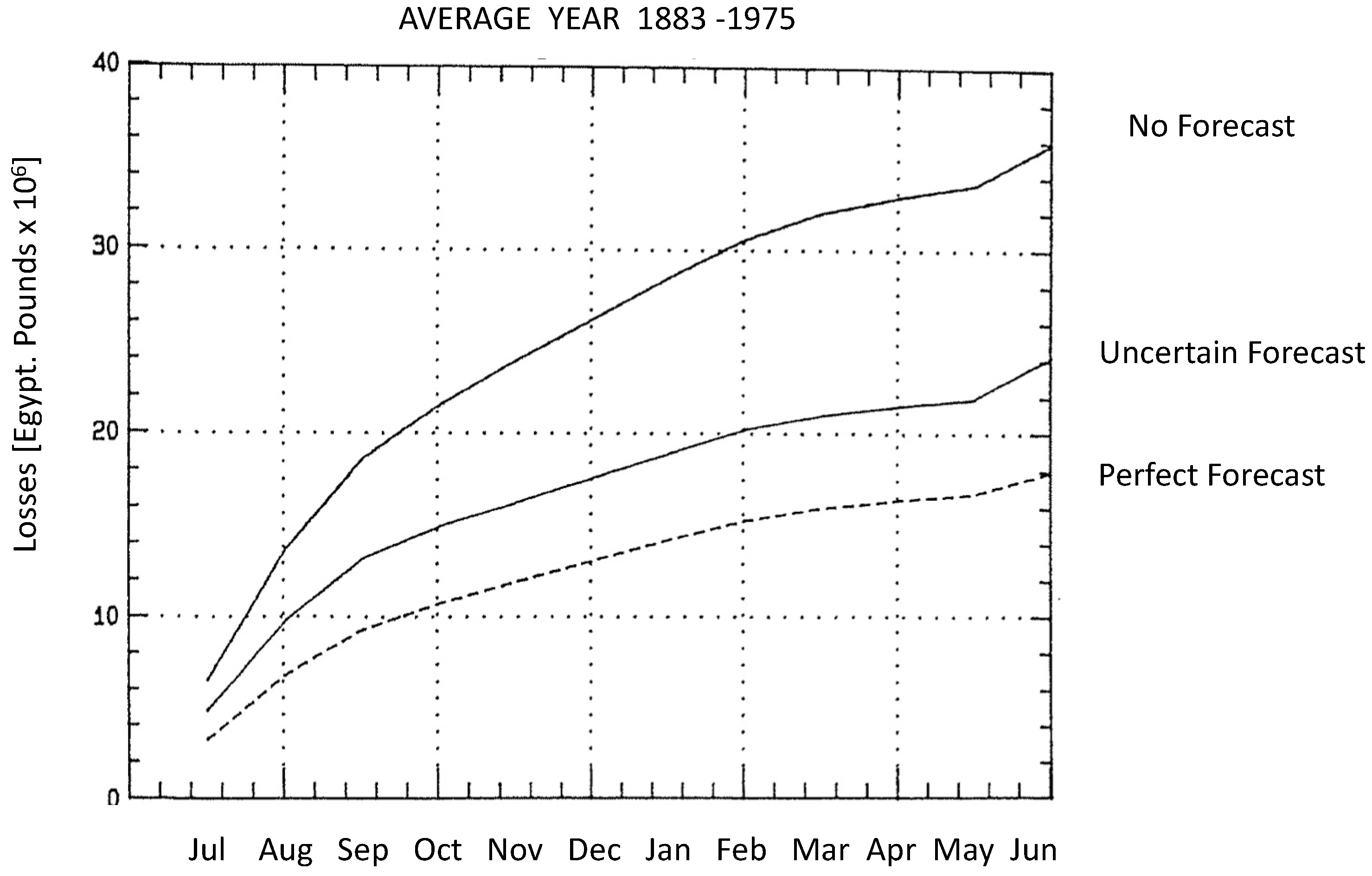
  3. Todini, E. Coupling real time forecasting in the Aswan Dam reservoir management. In Proceedings of the Workshop on Monitoring, Forecasting and Simulation of River Basins for Agricultural Production, FAO and Centro IDEA, Bologna, Italy, 18–23 March 1991; Land and Water Development Division, FAO: Rome, Italy, 1991. Report N. FAO-AGL-RAF/8969. [Google Scholar]
  4. Reggiani, P.; Todini, E.; Boyko, O.; Buizza, R. Assessing uncertainty for decision-making in climate adaptation and risk mitigation. Int. J. Clim. 2021, 41, 2891–2912. [Google Scholar] [CrossRef]
  5. Zadeh, L.A. Fuzzy sets. Inf. Control 1965, 8, 338–353. [Google Scholar] [CrossRef] [Green Version]
  6. Deng, J.L. Control problems of grey systems. Syst. Control Lett. 1982, 5, 288–294. [Google Scholar]
  7. Todini, E. The role of predictive uncertainty in the operational management of reservoirs. In Evolving Water Resources Systems: Understanding, Predicting and Managing Water–Society Interactions, 2014 Proceedings of ICWRS2014, Bologna, Italy, 4–6 June 2014; IAHS Publ. 36X; IAHS Press: Wallingford, UK, 2014. [Google Scholar] [CrossRef]
  8. Dirac, P.A.M. The Principles of Quantum Mechanics, 4th ed.; International Series of Monographs on Physics 27; Oxford University Press: New York, NY, USA, 1958; p. 328. ISBN 978-0-19-852011-5. [Google Scholar]
  9. Glahn, H.R.; Lowry, D.A. The Use of Model Output Statistics (MOS) in Objective Weather Forecasting. J. Appl. Meteorol. 1972, 11, 1203–1211. Available online: http://www.jstor.org/stable/26176961 (accessed on 28 June 2022). [CrossRef] [Green Version]
  10. Wilks, D.S. Statistical Methods in the Atmospheric Sciences: An Introduction; International Geophysics Series; Elsevier: San Diego, CA, USA, 1995; Volume 59, 467p. [Google Scholar]
  11. Raftery, A.E. Bayesian model selection in structural equation models. In Testing Structural Equation Models; Bollen, K.A., Long, J.S., Eds.; Sage: Newbury Park, CA, USA, 1993; pp. 163–180. [Google Scholar]
  12. Krzysztofowicz, R. Bayesian theory of probabilistic forecasting via deterministic hydrologic model. Water Resour. Res. 1999, 35, 2739–2750. [Google Scholar] [CrossRef] [Green Version]
  13. Koenker, R. Quantile Regression. In Econometric Society Monographs; Cambridge University Press: New York, NY, USA, 2005. [Google Scholar]
  14. Todini, E. A model conditional processor to assess predictive uncertainty in flood forecasting. Int. J. River Basin Manag. 2008, 6, 123–137. [Google Scholar] [CrossRef]
  15. Coccia, G.; Todini, E. Recent developments in predictive uncertainty assessment based on the model conditional processor approach. Hydrol. Earth Syst. Sci. 2011, 15, 3253–3274. [Google Scholar] [CrossRef] [Green Version]
  16. Coccia, G. Analysis and Developments of Uncertainty Processors for Real Time Flood Forecasting. Ph.D. Thesis, University of Bologna, Bologna, Italy, 2011. Available online: http://amsdottorato.unibo.it/id/eprint/3423 (accessed on 24 January 2019). [CrossRef]
  17. Krzysztofowicz, R. Probabilistic flood forecasts: Exact and approximate predictive distributions. J. Hydrol. 2014, 517, 643–651. [Google Scholar] [CrossRef]
  18. Barbetta, S.; Coccia, G.; Moramarco, T.; Brocca, L.; Todini, E. The multi temporal/multi-model approach to predictive uncertainty assessment in real-time flood forecasting. J. Hydrol. 2017, 551, 555–576. [Google Scholar] [CrossRef]
  19. Matthews, G.; Barnard, C.; Cloke, H.; Dance, S.L.; Jurlina, T.; Mazzetti, C.; Prudhomme, C. Evaluating the impact of post-processing medium-range ensemble streamflow forecasts from the European Flood Awareness System. Hydrol. Earth Syst. Sci. 2022, 26, 2939–2968. [Google Scholar] [CrossRef]
  20. Box, G.E.P.; Jenkins, G.M. Time Series Analysis: Forecasting and Control; Holden-Day: San Francisco, CA, USA, 1970. [Google Scholar]
  21. Wang, Q.; Shao, Y.; Song, Y.; Schepen, A.; Robertson, D.E.; Ryu, D.; Pappenberger, F. An evaluation of ECMWF SEAS5 seasonal climate forecasts for Australia using a new forecast calibration algorithm. Environ. Model. Softw. 2019, 122, 104550. [Google Scholar] [CrossRef]
  22. Gneiting, T.; Raftery, A.E.; Westveld, A.H.; Goldman, T. Calibrated Probabilistic Forecasting Using Ensemble Model Output Statistics and Minimum CRPS Estimation. Mon. Weather Rev. 2005, 133, 1098–1118. [Google Scholar] [CrossRef]
  23. Evensen, G. The Ensemble Kalman Filter: Theoretical formulation and practical implementation. Ocean Dyn. 2003, 53, 343–367. [Google Scholar] [CrossRef]
  24. IPCC. Climate Change 2013: The Physical Science Basis. Contribution of Working Group I to the Fifth Assessment Report of the Intergovernmental Panel on Climate Change; Cambridge University Press: Cambridge, UK; New York, NY, USA, 2013; Available online: https://www.climatechange2013.org (accessed on 28 June 2022).
  25. Meehl, G.A.; Boer, G.J.; Covey, C.; Latif, M.; Stouer, R.J. The coupled model inter-comparison project (CMIP). Bull. Am. Meteorol. Soc. 2000, 81, 313–318. [Google Scholar] [CrossRef] [Green Version]
  26. Meehl, G.A.; Covey, C.; Delworth, T.; Latif, M.; McAvaney, B.; Mitchell, J.F.B.; Stouffer, R.J.; Taylor, K.E. The WCRP CMIP3 multi-model dataset: A new era in climate change research. Bull. Am. Meteorol. Soc. 2007, 88, 1383–1394. [Google Scholar] [CrossRef] [Green Version]
  27. Taylor, K.E.; Stouer, R.J.; Meehl, G.A. Summary of the CMIP5 experiment design. Bull. Am. Meteorol. Soc. 2012, 93, 485–498. [Google Scholar] [CrossRef] [Green Version]
  28. Eyring, V.; Bony, S.; Meehl, G.A.; Senior, C.A.; Stevens, B.; Stouffer, R.J.; Taylor, K.E. Overview of the Coupled Model Intercomparison Project Phase 6 (CMIP6) experimental design and organization. Geosci. Model Dev. 2016, 9, 1937–1958. [Google Scholar] [CrossRef] [Green Version]
  29. Giorgi, F.; Francisco, R. Uncertainties in regional climate change prediction: A regional analysis of ensemble simulations with the HADCM2 coupled AOGCM. Clim. Dyn. 2000, 16, 169–182. [Google Scholar] [CrossRef]
  30. Palmer, T. Predicting uncertainty in forecasts of weather and climate. Rep. Prog. Phys. 2000, 63, 71–116. [Google Scholar] [CrossRef] [Green Version]
  31. Krzysztofowicz, R. The case for probabilistic forecasting in hydrology. J. Hydrol. 2001, 249, 2–9. [Google Scholar] [CrossRef]
  32. Hamill, T.M.; Whitaker, J.S. Probabilistic Quantitative Precipitation Forecasts Based on Reforecast Analogs: Theory and Application. Mon. Weather Rev. 2006, 134, 3209–3229. [Google Scholar] [CrossRef]
  33. Montanari, A. What do we mean by ‘uncertainty’? The need for a consistent wording about uncertainty assessment in hydrology. Hydrol. Process. 2007, 21, 841–845. [Google Scholar] [CrossRef]
  34. Beven, K.J.; Alcock, R.E. Modelling everything everywhere: A new approach to decision-making for water management under uncertainty. Freshw. Biol. 2011, 57, 124–132. [Google Scholar] [CrossRef] [Green Version]
  35. Beven, K.J. Facets of uncertainty: Epistemic uncertainty, non-stationarity, likelihood, hypothesis testing, and communication. Hydrol. Sci. J. 2016, 61, 1652–1665. [Google Scholar] [CrossRef] [Green Version]
  36. Clark, M.P.; Wilby, R.L.; Gutmann, E.D.; Vano, J.A.; Gangopadhyay, S.; Wood, A.W.; Fowler, H.J.; Prudhomme, C.; Arnold, J.R.; Brekke, L.D. Characterizing Uncertainty of the Hydrologic Impacts of Climate Change. Curr. Clim. Chang. Rep. 2016, 2, 55–64. [Google Scholar] [CrossRef] [Green Version]
  37. Draper, D.; Krnjajic, M. Calibration Results for Bayesian Model Specification; Technical Report; Department of Applied Mathematics and Statistics, University of California: Santa Cruz, CA, USA, 2013; Available online: https://users.soe.ucsc.edu/~draper/draper-krnjajic-2013-draft.pdf (accessed on 1 June 2022).
Figure 1. Losses by the Aswan reservoir accrued over one year, depending on the management strategy (reprinted from [3]). The thicker solid line (No Forecast) represents the results of management based on the historical monthly average Nile inflows; the dotted line represents the results of management based on the hypothetical knowledge of future inputs (Perfect Forecast); the thinner continuous line represents the results of a management based on imperfect knowledge of future inputs provided by a simple AR (1) (Uncertain Forecast) forecasting model, while accounting at each time step for the predictive probability distribution in estimating the volume to be released. Note that the information produced, even by a very simple model such as the AR(1), leads to significantly loss reduction (over 65%) by approaching the lower limit of losses obtainable with a perfect forecast, namely the retrospective perfect knowledge of future reservoir inflows [3].
Hydrology 09 00136 g001
Figure 2. The monthly non-stationary water levels of the Nile at Roda’s Nilometer (in cm) during the period 1871–1971 considered as a weakly stationary stochastic process. We identified two 20-year sub-periods. Within each period, the stochastic process could be thought of as weakly stationary and ergodic, while the process over the 100-year period was clearly non-stationary.
Hydrology 09 00136 g002
Figure 3. Comparison between the expected losses estimated (a) deterministically, according to the expected value of the volume forecast, and (b) probabilistically, by integrating the product between losses and their predictive probability of occurrence.
Hydrology 09 00136 g003
Figure 4. In pane (a), the representation of uncertainty, or rather our knowledge, in the form of probability density allows its informative use in decision-making schemes. In (b), where the expected value surrounded by the limits of ±   1 standard errors are plotted, only the information on the dispersion of the observations is provided, which gives a measure of the uncertainty, but does not allow us to use it in the decision-making phase.
Hydrology 09 00136 g004
Figure 5. The mathematical representation of knowledge: (a) perfect ignorance; (b) incomplete knowledge; (c) perfect knowledge.
Hydrology 09 00136 g005
Figure 6. Uncertainty in the evolution of a chaotic physical system (Real World) and its modeled representation (Virtual World of Models). In green the evolution from the current state to the actual future value (solid line) and to possible alternative future states (green zone). In red, the evolution of the current state to the expected value of the future state (solid line) while the evolution of the model’s predictions from the present to the future (orange zones), is not necessarily coinciding with the real future states (redrawn from [4]).
Hydrology 09 00136 g006
Figure 7. Baseline window and two predictive windows for the prost-processed CMIP5 RCP 4.5 temperature projections, river Po basin, Northern Italy. Seasonal mean observed temperature (blue), unprocessed ensemble output (pink), ensemble mean (light red) and post-processed predictive mean (flash red), spring (MAM). The grey-shaded areas indicate the 50% and 95% credible intervals (redrawn from [4]).
Hydrology 09 00136 g007
Figure 8. Baseline window and two predictive windows for the prost-processed CMIP5 RCP 8.5 precipitation projections, river Po basin, Northern Italy. The precipitation is given as average over a 1° × 1° reference cell centered in 10.08° E and 45.03° N. Seasonal mean observed precipitation (blue), unprocessed ensemble output (brown), ensemble mean (light red) and post-processed predictive mean (flash red), spring (MAM). The grey-shaded areas indicate the 50% and 95% credible intervals.
Hydrology 09 00136 g008
Figure 9. Probability density functions of observed and projected precipitation means (in mm) for a 1° × 1° reference cell centered in 8.08° E and 45.32° N, river Po basin, Northern Italy. Observations (blue dashed), post-processed control period (blue), prognostic window 2035–2065 (red) and 2070–2100 (green) projections, for the summer quarter June, July, August (JJA).
Hydrology 09 00136 g009
Figure 10. A simplified example of how a probabilistic forecast (thin black bell-shaped predictive density) can be used to derive appropriate decisions for reservoir releases. For a given probabilistic prediction (grey bell-shaped solid line), the expected loss, namely, the integral of the product of the density times the utility function of Equation (1) (solid thick black curve), is rather large. By releasing water, thus, reducing the volume in the reservoir, the probabilistic forecast of the cumulated volume is shifted downwards and is represented by the solid line bell shaped curve. As can be noticed, the expected utility value now becomes negligible. The appropriate amount to be released will then be found by comparing the expected utility function value to the cost of lack of future water availability (redrawn from [2]).
Hydrology 09 00136 g010
Publisher’s Note: MDPI stays neutral with regard to jurisdictional claims in published maps and institutional affiliations.

