Partial Desalination of Saline Groundwater, including Flowback Water, to Produce Irrigation Water

Abstract

Globally, more than 50 million ha of arable land is irrigated with saline water. The majority of this saline irrigation water is derived from saline groundwater. Global irrigation requirements may increase from 270 million ha in 2014 to about 750 million ha by 2050 as the global population increases to 9.1 billion people. The majority of this additional irrigation water is likely to come from saline groundwater sources. Desalination of irrigation water increases crop yield. A combination of high water volume requirements and low crop yields requires that, for widespread usage, the desalinated irrigation water product will require a delivery price of <USD 0.5 m³. This study considers five passive desalination routes (n-Fe⁰; n-Fe₃O₄; Fe⁰:Fe(b)@C⁰ polymer; n-Fe⁰:Fe(b) polymer; n-Fe(b) polymer) that may potentially achieve this goal: A common desalination mechanism is identified for the Fe⁰:Fe(b)@C⁰ polymer; n-Fe⁰:Fe(b) polymer; and n-Fe(b) polymer routes. The analysis establishes that the n-Fe(b) polymer route may be able to achieve (with a reaction time of 1 h) an 80% to 90% desalination of saline groundwater or flowback water (12.3 g NaCl L⁻¹; EC = 17.6 dSm⁻¹), to form partially desalinated irrigation water (1.2 to 2.4 g NaCl L⁻¹; EC = 2 to 3.4 dSm⁻¹) with an associated reduction in the sodium adsorption ratio (SAR) from 125 to between 1.2 and 2.5, for a potential material (n-Fe(b) polymer) treatment cost of <USD 0.01 m⁻³, after considering polymer reuse and recycle, but excluding all other plant and other operating costs. The examples demonstrate that the polymers can be used to create: (i) a desalinated stationary hydrodynamic plume, containing 47,123 m³ water (1 to 2.5 g NaCl L⁻¹), within 157,080 m³ porous rock forming a confined, saline aquifer (18.59 g NaCl L⁻¹), to act as a reservoir of desalinated water (96 m³ d⁻¹) for irrigation, with the potential to produce >960 m³ d⁻¹ as required; (ii) a desalinated, perched, stationary, shallow groundwater mound, located above the regional water table, containing >200 m³ of desalinated water.

1. Introduction

Global cropland comprises about 1724.08 million ha, of which about 403 million ha were irrigated during 2019 [1]. Water used for irrigation falls into two categories: (i) rainfall-derived water, which is termed green water [1]; and (ii) surface water + groundwater-derived water, which is termed blue water [1]. Globally, about 72.5% of cropland is rain fed, receiving about 8325.12 km³ a⁻¹ [1], The remaining 27.5% of global cropland is irrigated with blue water, about 1299.19 km³ a⁻¹ [1]. Blue water represents >87% of global consumptive water usage [1]. This consumption is currently split as follows: Asia 72.6% [1]; Africa 6.4% [1]; Europe 7.2% [1]; North America 10.8% [1]; Oceania 0.5% [1]; and South America 2.5% [1]. Total water consumption due to irrigation is 1131.04 km³ a⁻¹, of which 910.83 km³ a⁻¹ is used for crop irrigation [1].

One billion ha of land are adversely affected by salinization, including more than 20% of irrigated land (>80.6 million ha) [2]. Soil is considered to be saline when its electrical conductivity (EC) exceeds 4 dSm⁻¹ (4 mScm⁻¹) [2]. This equates to a pore-water salinity of about 2–2.6 g NaCl L⁻¹. Globally, about 21,368 million ha of salinized land has been identified as being potentially suitable for irrigation using saline or desalinated water [2]. Groundwater irrigation reduces overall global poverty but can increase socioeconomic vulnerability, particularly in arid and semi-arid regions [3].

Groundwater forms a primary buffer for anthropogenic domestic use, industrial use, municipal use, and agricultural use. In 2014, around 270 million ha of arable land was irrigated, of which about 89 million ha was irrigated directly from groundwater [4]. This irrigation requirement has been forecast to rise to >750 million ha by 2050, to assist in meeting the required increase in global food supply, as the global population rises from its current level of around 8 billion to a forecast level of around 9.1–9.9 billion by 2050 [4]. The bulk of the water required to meet the increased irrigation requirement is likely to be obtained from saline groundwater. Saline irrigation (water EC = 0.6 to 15.7 dSm⁻¹) reduces crop yields when compared with freshwater irrigation [5,6,7].

Once aquifer groundwater (or groundwater extracted from shale gas or shale oil wells (flowback water)) is used for irrigation, the associated overland flow and shallow groundwater flow are not returned to the primary originating aquifer. This can result in the depletion of the primary aquifer. Crop irrigation currently provides a low return on investment. While replacing saline irrigation water with desalinated water increases crop yields and the total crop sale value, the total return on investment decreases as the cost of the desalinated water increases [4,6,7].

The predicted increase in global irrigated land area between 2014 and 2050 implies that global consumptive water usage will rise from its current level of about 63% of current global water usage to more than 175% of current global water usage. The majority of this projected increase in water demand (14,300 km³ a⁻¹) is likely to be from saline groundwater.

1.1. Saline Groundwater Sources

Five types of saline groundwater are potentially available to meet this expected increase in water demand. They are: (i) aquifer groundwater abstracted from a borehole, this includes both fossil saline water [8,9,10,11] and groundwater, which is actively recharged by precipitation and riparian interactions [12,13,14,15]; (ii) associated water produced as a by-product of mining [16,17,18] or hydrocarbon production [19,20,21]; (iii) geothermal water produced as a by-product of geothermal energy extraction [22,23,24]; (iv), flowback water associated with oil shale and gas shale hydrocarbon extraction activities [25,26,27]; and (v) aquifer water in areas where the aquifer is subject to seawater incursion [28,29,30]. Additionally, in some areas, saline water may be available from tidally influenced riparian water [31] and saline lakes [32]. In many areas, prolonged irrigation has led to the salinization of both groundwater [33] and downstream lakes [34].

1.2. Desalination Solutions

A number of possible desalination solutions can be constructed for this saline groundwater, which are designed to create an increase in crop yield and an increase in the return on investment for the agricultural holder through the use of partially desalinated groundwater for irrigation. Desalination processes can use a physical process or a chemical process.

Conventional pressure-based desalination systems (e.g., reverse osmosis), thermal-based systems, and electrocoagulation systems can all produce an almost pure (desalinated) water product, but the removed Na⁺ and Cl^- ions are retained in a larger volume of waste (reject) brine, which requires disposal.

These systems are energy intensive and typically consume 3 to 6 m³ of water for each 1 m³ of product water. The residue is discharged as a waste brine. Conventional systems typically produce desalinated water for a cost of >USD 3 m⁻³, and for most agricultural crops, the increased revenue associated with the increased yield resulting from the use of purchased desalinated water is more than offset by the costs associated with purchasing desalinated water.

Since 2008, the patent and academic literature (Figure 1) has identified that passive (chemical) approaches (termed ZVI (zero valent iron) desalination) based on the use of Fe⁰, Feⁿ⁺, or Fe_xO_yH_z polymers (e.g., akageneite, green rust), Fe(a) polymers, Fe(b) polymers, Fe(c) polymers, or Fe-organic polymers could be used to partially desalinate water [4,6,7]. These studies have indicated that it may be possible to create solutions where the provision of partially desalinated water could cost between USD 0.1 and 3 m⁻³. These processes do not produce a reject brine waste product and can be operated without an external energy source. They may therefore create a situation that increases crop yields, increases the agricultural unit’s return on investment, and reduces the overall amount of water required to irrigate a specific acreage.

1.3. ZVI Desalination Considerations

This study considers how five different unsupported ZVI desalination approaches (n-Fe⁰; n-Fe₃O₄; Fe⁰:Fe(b)@C⁰ polymer; n-Fe⁰:Fe(b) polymer; n-Fe(b) polymer (Figure 1)) could be adapted to produce partially desalinated water from saline groundwater or saline flowback water, which may be suitable for irrigation. Two other supported ZVI desalination polymer approaches (Fe⁰:Fe(b)@Urea [4] and SiO₂@Fe(b)@Urea [7]) have been trialed at commercial scale and are not addressed further in this study. They are designed to catalytically convert Fe ions in the water into scavenging polymers (Fe(b,c)), which remove the NaCl from the water [7].

Commercial operation of the five different unsupported desalination approaches will require the use of a number of different reactor trains operating in parallel. The n-Fe(b)—Sol Gel polymers (Figure 1) are designed to be used in a multi-train reactor, which either involves a batch flow process or a continuous flow process. The polymer examples provided in this study are based on batch flow results.

Subsequent, ongoing commercial-scale experiments (utilizing the data from this study) are based on the design concept of a multi-tubular, transport line (moving bed) [35,36] reactor. The commercial-scale test reactors have a tube length of between 3 and 12 m and an outer diameter (O.D.) of 0.0423 m. Each tube has been trialed (in vertical, horizontal, and inclined orientations) at a continuous flow rate of up to 0.2 m³ h⁻¹ (4.3 m³ d⁻¹). A tube bundle of 100 tubes ((0.45 m × 0.45 m + baffle space) × 3 to 12 m length) will be expected to process >400 m³ d⁻¹. Commercial-scale reactors will be constructed using ABS (Acrylonitrile-butadiene-styrene) tubing (3 to 6 m lengths, 0.04–0.2 m O.D.; Class C, E, or T; BS5391; rated to 0.9 MPa and −40 °C to 70 °C) with ABS solvent weld joints and ABS pipe, flange, and valve fittings.

1.4. Production of Irrigation Quality Water

In many agricultural areas, freshwater aquifers are either reserved for domestic use or, when used for irrigation, have become depleted. In these areas, the primary remaining irrigation water source is saline groundwater. This has five impacts on agricultural land. They are: (i) the soil becomes progressively salinized; (ii) the crop yield (t ha⁻¹); (iii) the range of crop varieties that can be grown decreases progressively as the water salinity and soil salinization increase; (iv) the crop value may decrease, particularly with tomatoes, vegetables, and fruit, due to discoloration, skin thickening, and taste changes; (v) reduction in land value due to the reduced economic return from the land. In some cases, the land is rendered valueless and is abandoned, either as a direct result of salinization associated with saline irrigation or due to freshwater aquifer depletion (in areas where the saline aquifer is too saline to be considered an economic irrigation water source).

Irrigation is a major cause of groundwater depletion in many freshwater aquifers. This depletion results in (i) salinization of the soils, accompanied in some areas with a gradual deepening of both the salinization zone and the upper shallow perched (or regional) water table; (ii) a requirement to use saline water from saline groundwater aquifers for irrigation; (iii) a gradual salinization of freshwater aquifers in coastal areas due to seawater incursion. The salinization of this irrigation water, and irrigated soils, associated with agricultural intensification, results in an eventual reduction in agricultural economic activity within the area.

Most agricultural holdings are limited in size and do not have sufficient spare land to accommodate large scale tanks or impoundments (1000–60,000 m³) to accommodate the amount of irrigation water required for a few days’ irrigation. Irrigation requirements typically fall in the range of 1000 to 10,000 ha⁻¹.

The alternative to surface storage (with associated land sterilization) is to either store the desalinated water in a perched shallow groundwater mound or in a stationary hydrodynamic plume within a confined aquifer, located under the ground surface of the agricultural holding. This is the approach considered in this study.

This approach requires the construction of either a stationary hydrodynamic plume within a confined (or unconfined) saline aquifer or a perched shallow groundwater mound in salinized soil. This process desalinates both the salinized soil and aquifer contained within the groundwater mound or stationary plume. This creates a reservoir of mobile desalinated water that can be abstracted as required for irrigation.

A hydrodynamic stationary plume, or perched groundwater mound, is created using a combination of infiltration and abstraction wells, where water is continuously abstracted, desalinated, and reinfiltrated (Figure 2). The hydrodynamic concepts were originally developed in the hydrocarbon industry to both search for hydrodynamically trapped hydrocarbon accumulations and enhance the proportion of mobile hydrocarbon recovered from aquifers.

The results from this study could be used to actively desalinate and reverse the impact of seawater incursion into the groundwater associated with freshwater aquifers.

1.5. Desalination Decision

The decision as to whether to use a batch of desalinated water for irrigation is complex (Figure 2). Once the ZVI desalination technology has been selected and the stationary hydrodynamic plume or perched groundwater mound has been created (Figure 2), the abstracted desalinated water is then checked to determine:

• The expected crop yield and value following the use of the water;
• The expected costs associated with using the water,
• Whether the water complies with local regulations in terms of its chemistry and water quality indicators. Most global regulators have standards that have to be complied with.

2. Terminology, Materials and Methods

2.1. ZVI Terminology, Groundwater Salinity Indices and Patent Terminology

2.1.1. ZVI Definition

The term ZVI is used in this study as a generic basket term to include Fe⁰, Fe_xO_y, FeOOH, Fe_xO_yH_z, Fe inorganic polymers, and Fe-organic polymers. The term Fe⁰ is used in this study to refer to native iron metal. The suffix “n-“denotes a nano-sized-particle, typically between 10 and 100 nm. The suffix “m-“denotes a micron-sized-particle, typically between 1 and 100 microns.

2.1.2. Patent Terminology

Patents are referred to in the text by their patent number. The prefixes used are US = US patent; ES = Spanish patent; FR = French patent; GB = UK patent; TW = Taiwan patent; JP = Japanese patent; and CH = Chinese patent. The standard patent number end terminology is: Letter [A] = application; Letter [B] = awarded patent following examination.

2.1.3. Desalination Pattern Classification

A classification of the different patterns of changing salinity with time that have been observed over the last 14 years associated with ZVI desalination is provided in Appendix B.

2.1.4. Salinity Indices

The various molar geochemical indices, which are used to describe groundwater’s suitability for irrigation water, are summarized in Appendix C. The Sodium Adsorption Ratio (SAR) is the most widely used. ZVI desalination reduces the various indices by reducing the amount of Na⁺ and Cl^- ions in the irrigation (product) water. The sol-gel approaches (Figure 1) may also decrease the various indices by increasing the availability of Ca²⁺ ions in the irrigation (product) water.

2.2. Assessment of Crop Yield Resulting from the Use of Partially Desalinated Irrigation Water

Desalinated (or partially desalinated) irrigation water, when used in place of saline irrigation water, results in an increase in crop yield, a decrease in soil salinization, a decrease in soil waterlogging, and it may result in an increase in crop quality [4,6,7]. The exact yield increase resulting from desalination is a function of crop type, farming practice, soil conditions, crop variety, and climatic conditions.

Yield Increase Assessment Methodology

A simple, easy-to-use screening method for assessing the relative increase in crop yield resulting from the use of partially desalinated irrigation is provided in references [4,7]. The final example in this study takes feed water with a salinity of 12.3 g NaCl L⁻¹; EC = 17.6 dSm⁻¹ to form partially desalinated irrigation water (1.2 to 2.4 g NaCl L⁻¹; EC = 2 to 3.4 dSm⁻¹). This was accompanied by an associated reduction in the sodium adsorption ratio (SAR) from 125 to between 1.2 and 2.5.

The method described in Reference [7] indicates that if this saline (flowback or groundwater-sourced) water (12.3 g L⁻¹) was used for irrigation, then only a few crops may provide a meaningful crop yield (e.g., sugar beet and wheat [7]). Reducing the irrigation water salinity to 1.5 g L⁻¹ would be expected [7] to increase sugar beet yields by 236% and wheat yields by 414%. It would also allow the area to be used (subject to soil conditions and climate) to grow the majority of crops that can be grown in an area receiving freshwater irrigation [7].

Reducing irrigation water salinity will therefore have benefits associated with:

• Increased crop yield and increased gross revenue;
• Increased choice of crops which can be grown on a holding; and
• Increased agricultural land value.

2.3. Polymer Terminology

2.3.1. Initial Polymer Product

Feⁿ⁺ ions in the presence of Na⁺, OH^-, and Cl^- ions initially produce dimers with edge-shaped and corner-shaped octahedral sites [37]. After a short period (about 1 h), distinct trimers are associated with these sites, and coalescence of the trimmers results in the formation of β-FeOOH type polymers [37]. The rate of formation is a function of the NaOH:Feⁿ⁺ ratio (r) in the water at the reaction onset [37]. For r > 1.5, the hydrated polymers are stable and have a similar structure to β-FeOOH [37].

β-FeOOH type polymers are formed when Fe³⁺ ions are mixed with Cl^- ions and one or more of OH^- ions, HCO₃^- ions, and CO₃^2- ions [JP2018020920A; JP2018030748A]. The manufacturing process can require an increase in pH [US20120315479A1]. Individual β-FeOOH type crystallites have a width of 15–18 nm and a length of 100–200 nm [US20120315479A1]. β-FeOOH type polymers can incorporate Mn and Ca ions [US8313653B2].

2.3.2. Polymer Characterization

The characterization of the polymeric desalination catalyst, produced from n-Fe⁰ and Feⁿ⁺ ions, in terms of detailed chemical analyses and detailed morphology, is outside of the scope of this study.

2.3.3. Polymer Terminology

The following polymer terminology is used [38,39,40]. M = metal. M(a), Fe(a), Ca(a), Zn(a) = mononuclear hydroxyl complexes, e.g., HZnOH²⁺, HCaOH²⁺, HFeOH²⁺, HFeOH³⁺, Fe³⁺, Fe(OH)²⁺, Fe(OH)₂⁺, Fe(OH)₃, Fe(OH)₄⁻ (Fe₂(OH)₂⁴⁺ and Fe₃(OH)₄⁵⁺), some small polymers, and instantaneous reaction products. M(b) = polynuclear hydroxyl complexes with medium and high molecular masses, e.g., Fe(OH)₂⁴⁺; Fe(O₂H₆)³⁺; Fe₃(OH)₄⁵⁺; Fe₅(OH)₉⁶⁺, etc. M(c) = larger polymer or colloidal species, which include inert macromolecular coagulation of the forms M(OH)_x and MOOH. In practice, most metal polymers are a mixture of M(a) + M(b) + M(c). [@] signifies physical adsorption on a surface [7]; [:] signifies chemical adsorption on a surface [7].

2.4. ZVI Desalination Measurement

ZVI desalination is observed by comparing the feed water and product water using one or more of the following instruments and methods:

• Electrical conductivity (EC, mScm⁻¹, dSm⁻¹);
• Ion Selective Electrodes (ISE) for Na⁺ ions and Cl^- ions;
• Evaporation of product and feed waters to produce a residual measurable product;
• Ion chromatography and spectroscopy to identify Na⁺ and Cl^- ions;
• Flame emission photometry to identify Na⁺ ions
• Chemical titration to identify Cl^- ions;

The most common tool used globally to measure salinity is the EC. In this study, the primary tools used to measure salinity are Na⁺ ISE and Cl^- ISE. Confirmation or corroboration of the ISE results is provided by both EC and evaporation analyses.

2.4.1. Desalination Assessment

Desalination (D_s), as a fraction of the feed concentration, is determined as:

D_s = 1 − (C_{t = n}/C_{t = 0}),

(1)

C_{t= n} = ion concentration in the product water at time t = n; C_{t = 0} = ion concentration in the feed water at time t = 0.

2.4.2. Relationship between EC and Salinity

EC varies with water salinity but is also influenced by the conductivity of other ion components in the water, where [41]:

NaCl, g L⁻¹ = F (EC),

(2)

F = a constant. F is commonly stated [41] as being in the range of 0.50 to 0.55 for NaCl determination in most EC meter instruction booklets. Chemical tables [42] suggest that the actual relationship between F and EC in pure saline water is:

F = 0.001967(EC) + 0.605453,

(3)

Each ion present in the water provides a contribution to EC [42]. It follows that if two components are present and the desalination process only removes one component, then the resultant product EC at time t = n, will be determined as:

EC_{t = n} = EC_{t = 0} − EC attributable to removed NaCl,

(4)

Consequently, the amount of desalination indicated by an ISE can be higher than desalination measured by an EC when significant concentrations of other ions are present. Most water contains a multiplicity of ion components. Each component has its own value of F.

The other principal dissolved components in saline water are: Na₂SO₄ (F = 0.9732EC [42]) KCl (F = 0.6646EC [42]), CaCl₂ (F = 0.6677EC [42]), Na₂CO₃ (F = 0.878EC [42]), MgSO₄ (F = 1.4416EC [42]), and MgCl₃ (F = 0.6296EC [42]). Organic acids, when present, have high values of F. For example: HCOOH (F = 5.0576EC [42]), CH₃COOH (F = 21.56EC [42]), H₂C₂O₄ (F = 0.5184EC [42]), and H₃C(OH)(COO)₃ (F = 5.5856EC [42]). Organic species, when present, have a disproportionate impact on the EC. Sulphates, when present in significant quantities, can increase F into the range of 0.9 to 1.7 [42]. Carbonates, when present in significant quantities, can increase F into the range of 0.8 to 1.0 [42]. Hydroxides, when present in significant quantities, can reduce F into the range of 0.2 to 0.5 [42].

Since most water is composite, the EC is normally used to define total dissolved solids (TDS) [41], where TDS, g L⁻¹ = F(EC). In the absence of any compositional data, F is commonly set at 0.55 to determine TDS [41]. In most saline water, the concentration of NaCl may represent >95% of the dissolved solids. In these circumstances, the EC becomes a proxy indicator of salinity.

The addition of Fe⁰ to acidic water results in the release of Feⁿ⁺ ions [43,44]. This release is accompanied by an increase in the EC, which can mask any decline in Na⁺ ion and Cl^- ion concentrations [44]. Consequently, the preferred instrument for salinity measurement in this study is an ISE.

Detailed analyses of TDS (20–292 g L⁻¹) in groundwater brines [45] have established that the relationship between TDS and EC for a saline water body typically follows a polynomial function, where:

TDS = a(EC)⁴ + b(EC)³ + c(EC)² + d(EC) + e,

(5)

a to e = polynomial constants that are specific to a water body. In pure sodium chloride solution, the relationship is considered to be exponential [45]:

TDS = a e ^b(EC),

(6)

a and b are exponential constants. The relative concentrations of monovalent and divalent ions in the water have a significant impact on EC [45]. Brine EC, for a specific TDS, decreases as the ratio of monovalent: divalent ions in the water decreases [45].

2.4.3. Significance of Fe⁰ Dissolution to Feⁿ⁺ ions

The dissolution of Fe⁰ to form Feⁿ⁺ ions and associated polymers can be a zero-order reaction [46]. A zero-order reaction is described [6,7] by regression equations of the form:

C_{t= n}/C_{t =0} = k_dissolution × t + [b],

(7)

C_{t= n} = k_dissolution × t + [C_{t = 0}],

(8)

where C_{t = n} = Fe⁰ concentration at time t = n; C_{t = 0} = initial Fe⁰ concentration; t = reaction time; [b] = a constant; k_dissolution = the Fe⁰ dissolution rate constant, for the reaction: Fe⁰ = Feⁿ⁺ + ne^-; C_{t = n}/C_{t = 0} = normalized, or fractional proportion of the original Fe⁰ charge left at time t = n.

2.4.4. Uncoated Fe⁰

Uncoated Fe⁰ (Figure 3) will dissolve (rust) rapidly in water [44,46]. The rate of dissolution is a function of the water composition, temperature, particle size, and particle shape. The zero-order kinetic data [46] for uncoated steel wool dissolution (unadjusted for coating retardation) provides a reasonable indication of the dissolution rates, which might be expected for uncoated n-Fe⁰ (Figure 3).

Uncoated n-Fe⁰ is expected to have a rate of dissolution (and Fe(a,b,c) polymer formation), which is greater than that associated with the median value and perhaps greater than the 3rd quartile (Figure 3). Therefore, if polymer formation (Figure 1) is associated with NaCl removal [4,6,7], then uncoated n-Fe⁰, or functionalized n-Fe⁰ may be required in order to achieve an economic desalination rate.

Figure 3c provides the Eh and pH of a continuous flow of water over 77 days through two fixed bed tubular (0.04 m O.D.) reactors. Reactor 1 contained 0.5 kg m-Fe⁰ (0.02 to 0.08 mm, flow rate, Q_A = 0.9 L h⁻¹). Reactor 2 contained 0.4 kg Fe⁰ (>1 mm, Q_A = 8 L h⁻¹). In both examples, the average product water Eh dropped and the pH increased relative to the feed water.

The bulk of the product water associated with the Fe⁰ (Reactor 2) remained in the Fe²⁺ stability zone [45,46,47,48,49,50] at around the Fe(b) polymer:Fe²⁺ redox fence, indicating that a net dissolution of Fe⁰ was expected and that only part of the dissolved Fe⁰ would be converted to polymer. Oxygenated flow lines and tanks associated with this water are coated with orange Fe(c) polymers (Fe(OH)₃, FeOOH). The bulk of the product water associated with the m-Fe⁰ (Reactor 1) remained in the Fe(b) polymer stability zone [47,48,49,50,51,52]. No dissolved Fe²⁼ ions were detected in the product water. In each example (Figure 2d), the product water was in Hydrogen Stability Zone 0 [52,53], indicating oxygenated conditions. It has been established that: (i) combining Fe⁰ with Al⁰ in saline water can move the metal bed into Hydrogen Stability Zone 2 [52,53]; (ii) decreasing the Fe⁰ particle size increases the pH of the product water. The pH shift moves the water into the H₂O₂ stability zone [52,54] (Figure 2e). This potentially allows Fenton remediation reactions to occur [55].

2.4.5. Coated Fe⁰

Coated n-Fe⁰ (Figure 3f) is expected to have a rate of dissolution and polymer formation that is substantially less than that associated with the 1st quartile (Figure 1). Therefore, if polymer formation is associated with NaCl removal [4,6,7], coated n-Fe⁰ will form a slow-reacting, useful evaluation tool to allow the desalination pattern to be monitored. In this study, it is used to determine if NaCl removal by coated n-Fe⁰ can be described as a zero-order reaction or a first-order reaction.

Coatings can take a number of forms and are placed on the nanoparticles for a number of different reasons. The principal reasons are: (i) to make the particles air stable, and to inhibit oxidation (e.g., TW201504159A; US10329179B2); This coating can be Fe₃O₄ (magnetite (US10329179B2)); activated carbon (e.g., US11103854B2; CN109305684B); tetraethyl orthosilicate (TEOS (US20130058724A1)); ethyl triethoxysilane (ETES (US20130058724A1)); (ii) to prevent the particles from corroding, when placed in water; (iii) add functional sites to the particle surface to aid selectivity and ion removal; (iv) control the dispersibility of nanoparticles to prevent clumping (e.g., US7635236B2). Coated n-Fe⁰ is commonly termed stabilized zero-valent iron nanoparticles. Detailed discussion of Fe⁰ coating approaches, coating types, and functionalized Fe⁰ is outside the scope of this study.

2.5. Desalination Mechanism

The ZVI desalination mechanism is unknown [7]. A number of different hypotheses have been developed. The desalination models used in the 2008/20015 patents (Figure 1) are different from those currently being developed for polymers. Each model will be addressed in this study. The current working model [7] for desalination using polymers is that:

• Fe⁰ surfaces corrode to form Fe_xO_yH_z species and release Feⁿ⁺ ions [56];
• The Feⁿ⁺ ions and Fe_xO_yH_z species interact with the water to form entrained polymer monomers (Fe(a), or Fe(b) or Fe(c)) [4,6,7,56];
• The polymer monomers aggregate to form fluid-filled entrained colloidal spheres [7,39];
• The spheres actively adsorb Na⁺ and Cl^- ions from the water and sequester them within the colloidal structures [6,7,56]. This process creates a zero-order pattern of ion removal [57,58] in Fe⁰:Fe(b)@C⁰ polymer desalination pellets [6,7,59], where:

C_{t = n} = k_obs t_r + C_t = ₀,

(9)

where k_obs = observed rate constant; t_r = reaction time. A first-order pattern of ion removal [57,58] is associated with n-Fe⁰, and both supported and unsupported sol-gel metal polymers [59], where:

Ln[C_{t = n}] = k_obs t_r + Ln[C_t = ₀],

(10)

• The colloidal structure breaks down to produce an amorphous polymer containing dead end porosity, which can include fluids contained within the former colloidal structure [6,59].

This study investigates this morphological desalination model further using n-Fe⁰:Fe(b) and n-Fe(b) polymers (Figure 1).

2.6. Desalination Pattern

The main ion removal patterns observed over the last 14 years are summarized in Appendix B. Each segment of the decline pattern can be defined in terms of a reaction of a specific order [59]. The reason why a decline pattern is not a simple zero, first, second, or higher order reaction [57,58] is unknown. The reason why a specific pattern develops is unknown. The common pattern is composite.

In most instances:

• A plot of ion concentration at time t = n (C_{t = n}) versus reaction time, t_r, or a plot of Ln(C_{t = n}) versus t_r, will equate to a straight line for each time segment, where C_{t = n} either declines with time, or increases with time, indicating that the reaction is zero-order, or pseudo-zero order, or first-order, or pseudo-first order [6,7,59,60].
• A plot of Ln(C_{t = n}/C_{t = 0}) versus t_r, can be described using a trendline regression equation [7,59], e.g.,:

  ∘

  Power function observed [7,59]

  Ln(C_{t = n}/C_{t = 0}) = [a] [t_r][b],

  (11)

  ∘

  Linear function observed [7]

  Ln(C_{t = n}/C_{t = 0}) = [a] [t_r] + [b],

  (12)

  ∘

  Logarithmic function observed [7]

  Ln(C_{t = n}/C_{t = 0}) = [a] Ln([t_r]) + [b],

  (13)

  ∘

  Exponential function observed [7]

  Ln(C_{t = n}/C_{t = 0}) = [a] e([tr])[b],

  (14)

where [a] and [b] are regression constants. [t_r] = time. In this study, the sol-gel, n-Fe(b) polymers remove N^a+ and Cl^- ions using a power function.

2.7. Statistical Methodology Used

The measured data was collated and processed in accordance with the methodology defined by the British Standards Institute [61]. Regression trend lines and associated statistics were calculated in MS Excel 2019. The Monte Carlo analyses were undertaken in MS Excel using the @Rand() random number generator function to generate values between 0 and 1. The polynomial equations, linear equations, and power equations were generated using the Trendline function in MS Excel.

The coefficient of determination, R², is the square of the Pearson Correlation Coefficient (PCC). By definition, R² falls within the range 1 and 0, and PCC falls between +1 and −1 [62,63]. The following interpretations are made [62,63]:

• PCC = 0.9 to 1.0 (R² = 0.81 to 1.00): Interpretation = very strong correlation
• PCC = 0.7 to 0.89 (R² = 0.49 to 0.79): Interpretation = strong correlation
• PCC = 0.4 to 0.69 (R² = 0.16 to 0.47): Interpretation = moderate correlation
• PCC = 0.1 to 0.39 (R² = 0.01 to 0.15): Interpretation = weak correlation
• PCC = 0.0 to 0.10 (R² = 0.00 to 0.01): Interpretation = negligible correlation

2.8. Data

The data generated by this study is provided in the text tables and figures.

2.9. Measurement Equipment

The instruments used were:

• ORP (oxidation reduction potential) meter (HM Digital) calibrated at ORP = 200 mV; Measured ORP (oxidation reduction potential) values are converted to Eh, mV as: Eh, mV = −65.667pH + 744.67 + ORP (mV), using a quinhydrone calibration at pH = 4 and pH = 7.
• pH meter (HM Digital) calibrated at pH = 4.01; 7.0; 10.0.
• EC (electrical conductivity) meter (HM Digital meter calibrated at EC = 1.431 mScm⁻¹).
• Cl^- ISE (Ion Selective Electrode); Bante Cl^- ISE, EDT Flow Plus Combination Cl^- ISE; Cole Parmer Cl^- ISE attached to a Bante 931 Ion meter. Calibration was undertaken using 0.001, 0.01, 0.1, and 1.0 M NaCl calibration solutions.
• Na⁺ ISE (Ion Selective Electrode); Bante Na ISE, Sciquip Na ISE, Cole Parmer Na ISE attached to a Bante 931 Ion Meter. Calibration was undertaken using 0.001, 0.01, 0.1, and 1.0 M NaCl calibration solutions.
• Temperature measurements, were made using a temperature probe, attached to a Bante 931 Ion Meter.

2.10. Reactor Size Used

The standard reactor size used was 1 L for n-Fe⁰ studies and 2.3 L for polymer studies. The reactor was operated as a static flow, static diffusion, and batch reactor. Operating pressure = atmospheric. Operating temperature = external environment temperature. This varies with the time of year and the time of day. At the site location, the operating temperature range was between 0 °C and 25 °C.

2.11. Materials Used

The saline water used was either seawater extracted from the North Sea at Blackness Castle, Firth of Forth, Scotland, or fresh water containing dissolved halite. The halite was purchased from Wickes Ltd., Perth, Scotland, UK.

The [FeSO₄ [H₂O]₇], MgCO₃, CaO, K₂CO₃, MnO₂, ZnO, urea, and tartaric acid powders, together with the formic acid used in this study were purchased from a variety of UK-based commercial agricultural and chemical suppliers.

2.12. Hydrology of a Stationary Plume

The desalination results are used to reconstruct the salinity of a saline aquifer by creating a stationary hydrodynamic plume within the aquifer. The hydrological and hydrodynamic equations and modeled examples are provided in Appendix D.

2.13. Past ZVI Desalination Processes

The ZVI desalination processes, n-Fe⁰; n-Fe₃O₄, and Fe⁰:Fe(b)@C⁰ are addressed in Appendix A. This analysis provides the technical background to the analysis of n-Fe⁰:Fe(a,b,c) and n-Fe(a,b,c) polymers undertaken in this study.

3. n-Fe⁰:Fe(a,b,c) Polymers

The analysis (Appendix A) of the existing n-Fe⁰ desalination route (Figure 1) indicated the presence of substantial technical and economic barriers, which need to be addressed prior to being able to economically utilize n-Fe⁰ to produce partially desalinated irrigation water from saline groundwater. Placement of n-Fe⁰ in water will result in the formation of n-Fe⁰:Fe(a,b,c) polymers and Fe(a,b,c) polymers [6,7,59]. In saline water, the dominant polymers are hydrated variations of the minerals green rust chloride and akageneite. Conventional ZVI water remediation theory does not consider that these polymers are active in the water remediation process; instead, it assumes that the n-Fe⁰ acts as an electron donor to effect remediation [64]. The polymer shell (Figure 3f) is commonly ignored or considered not to be involved in the remediation process [64]. This study considers that the polymer shell plays an active part in the desalination process [4,6,7].

This study reconfigures the conventional n-Fe⁰ desalination model and process (Appendix A) from a general circular process (Figure 4) of desalination followed by magnetic recovery, followed by reprocessing and regeneration, followed by reuse with makeup as appropriate, to a general circular process (Figure 4) of desalination, followed by gravity separation, followed by washing and separation, followed by reuse of the recovered iron polymers.

This section considers desalination using a modified version of the conventional n-Fe⁰ desalination process (Figure 4). The conventional model assumes that the functionalized sites are located on the n-Fe⁰ surface (Appendix A). In this study, it is assumed that the functionalized sites are located on the n-Fe polymer surfaces (Appendix A).

3.1. Functionalized Fe-Polymer Colloids

The functionalized, entrained, and corroding n-Fe⁰ particle aggregates by a form of snowball accretion to form agglomerated, colloidal nodules, constructed from n-Fe polymers. A typical example is provided in Figure 5a. Each of these nodules forms and grows by the accretion of fluid-filled colloidal spheres of n-Fe⁰:Fe(a,b,c) (Figure 5b). In the example illustrated in Figure 5, the average colloid sphere outer diameter was 0.0031 mm (3.1 microns); inner diameter was 0.002 mm; (outer volume = 1.56 × 10⁻⁸ mm³; inner (fluid) volume = 4.19 × 10⁻⁹ mm³; n-Fe⁰:Fe(a,b,c) rim volume = 1.14 × 10⁻⁸ mm³; n-Fe⁰:Fe(a,b,c) rim thickness = 0.00055 mm; sphere porosity = 26.8%).

3.2. Possible Ion Transport Model

If the m-Fe⁰:Fe(a,b,c)@C⁰ polymers [6] extract ions from one water surface and then transport the ions through the polymer to another water or fluid surface (e.g., Appendix D), then the fluid volumes within the fluid-filled colloid spheres (dead-end pores (Figure 5b)), may act as sinks for ion removal [59].

3.3. Fe:Fe(a,b,c) Polymer Spheres

If the n-Fe⁰ is placed in freshwater, it forms amorphous, flocculate aggregates (Figure 6a). In saline water, initially, the n-Fe⁰ aggregates to form hydrogen + water-filled n -Fe⁰:Fe(a,b,c) polymer spheres (Figure 6b), where within the sphere:

H₂O = OH^- + H⁺ = OH^● + 0.5H₂,

(15)

This set of reactions results in a charged internal surface at the fluid-polymer interface, e.g.,

2[n-Fe⁰:Fe(a,b,c)] + H₂O = [n-Fe⁰:Fe(a,b,c)@OH^-] + [n-Fe⁰:Fe(a,b,c)@H⁺],

(16)

[n-Fe⁰:Fe(a,b,c)] + H₂O = [n-Fe⁰:Fe(a,b,c)@OH^●] + H_2(gas),

(17)

3.4. Colloidal Spheres

The initial n-Fe⁰:Fe(b) colloidal spheres have a strong optical refraction contrast between the fluid in the spheres, the water body, and the sphere rim (Figure 6b). This is due to the presence of hydrogen within the spheres. Spheres, where the microscope optics are focused on the sphere center, have a doughnut-like appearance, as the sphere walls above the core are effectively transparent. There is a weak positive statistical trend between sphere diameter and the diameter of the encapsulated fluid core (Figure 7a).

3.5. Colloidal Sphere Diameter

For any specific sphere diameter, there is a wide range of internal fluid core diameters (Figure 7a). There is a positive linear relationship (Figure 7b) between sphere diameter and the thickness of the polymer rim surrounding the internal fluid core. There is a very weakly positive relationship between the sphere diameter and the volume of the internal fluid core (Figure 7c). This probably results from the formation of hydrogen, as the conversion of 1 mole of water to hydrogen will create an increase from 18 cm³ to 11,200 cm³.

3.6. Fluid Core Volume of the Spheres

Each observed doubling in the volume of the internal fluid core could be explained if 0.16% of the water in the fluid core (before the volume increase) was converted to hydrogen. This interpretation indicates that the principal control on the volume of the fluid core is the formation of hydrogen. Hydrogen gas generation by the n-Fe⁰ is therefore essential to increase the volume of dead-end porosity (Figure 7c) and the dead-end porosity as a proportion of total sphere volume (Figure 7d). It will also increase sphere buoyancy and sphere mobility, allowing spheres to aggregate and grow by accretion.

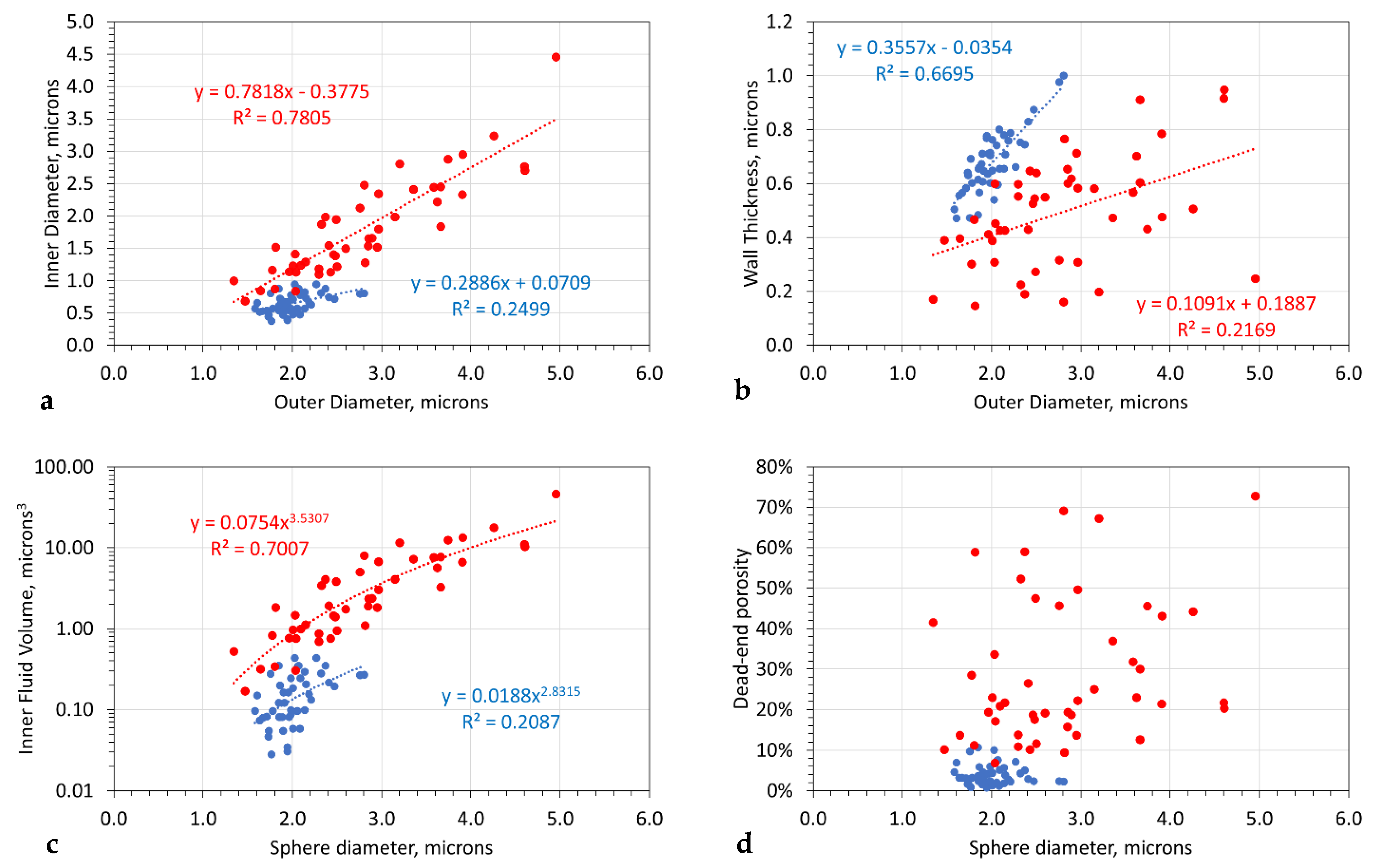
3.7. Change in Sphere Rim Thickness with Time

Analysis of entrained n-Fe⁰:Fe(a,b,c) polymers (Figure 6c) following extraction from saline water after 4000 h established (Figure 6c) that the entrained particles comprised thin-walled spheres containing solid minerals (NaCl, CaCl₂, NaHCO₃, CaCO₃, and NaOH) adsorbed from the water.

If the spheres produced after 2 h (Figure 7b) are compared with those present after 4000 h (Figure 6c), the following observations can be made:

• For a sphere with a specific outer diameter, the inner diameter of the fluid sphere increases with time (Figure 7a);
• The average sphere outer diameter and the sphere size range increase with time (Figure 7a);
• The average sphere wall thickness, when formed, shows a distinct positive correlation between outer diameter and wall thickness (Figure 7b); as time increases, the wall thickness observed for a specific outer diameter decreases relative to the initial regression trend line (Figure 7b);
• Increasing reaction time results in an increase in the internal fluid volume of the spheres and a positive correlation developing between internal fluid volume and sphere size (Figure 7c);
• After about 2 h, the typical sphere has a fluid volume of <10% (Figure 7d); this fluid volume (as a proportion of the sphere volume) can increase to >70% as the sphere grows (Figure 7d).
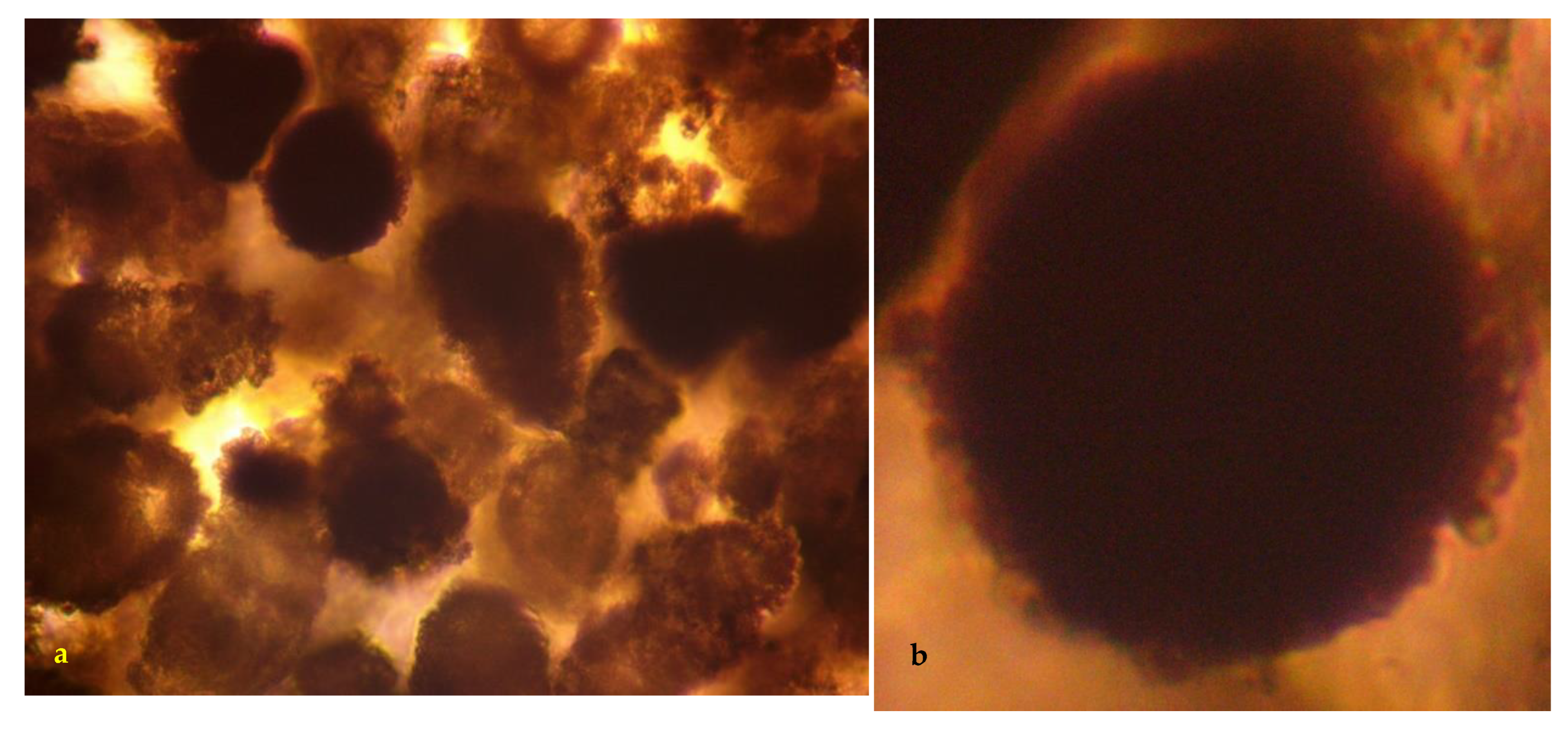
• After 4000 h, the spheres appear to be completely mineralized (Figure 6c).

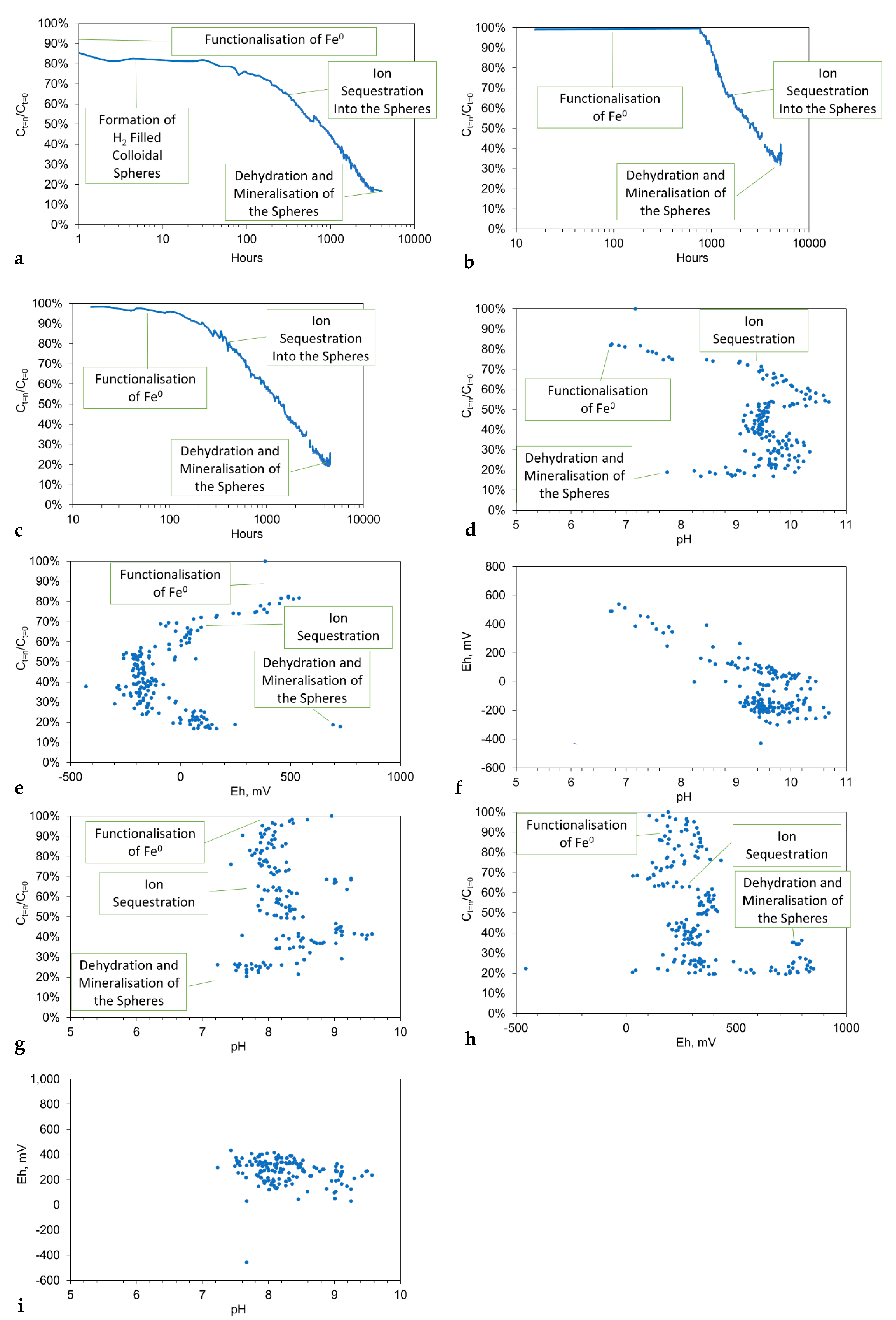
3.8. Model for Desalination by the Polymer Spheres

Comparison of the removal of NaCl from the feed water (Figure 8a–c) with the sphere morphology (Figure 7) suggests that desalination occurs in a number of phases:

• The initial functionalization of the n-Fe⁰ is associated with a pH shift into the range 8.5 to 11, and a decrease in Eh (Figure 8d–f);
• The trend of decreasing salinity continues while the pH remains in the range of 9 to 11, and the Eh is below 0 mV (Figure 8d–f);
• The cessation of salinity removal is associated with a decrease in pH into the range of 7 to 9, combined with an increase in Eh (Figure 8d–f).
• The removal of NaCl occurs in the redox (Eh:pH) regime, where the dominant Fe oxidation number is 3 (Figure 8d–f). This redox regime is consistent with desalination being associated with nFe⁰:n-Fe(a,b,c) polymers.

This analysis indicates that in saline water, the dominant method of ion removal may be in metal polymer colloidal spheres.

3.9. Reuse of n-Fe⁰

If the conventional n-Fe⁰ model is correct (Appendix D), the presence of corrosion products on the recovered n-Fe⁰ will result, if the recovered n-Fe⁰ is reused, in the amount of observed desalination progressively decreasing with time, as the corroding n-Fe⁰ becomes covered in Fe polymers.

This hypothesis was tested using gravity separation to recover a batch of n-Fe⁰ following use (Figure 8b). The recovered n-Fe⁰ + Fe polymers were not magnetic. This indicated that the bulk of the initial magnetic n-Fe⁰ charge had corroded to form polymers during the desalination process.

The recovered n-Fe⁰ was reused (Figure 8c). This reused n-Fe⁰ resulted in a lower increase in pH and a lower decrease in Eh during the desalination phase (Figure 8g,h). The redox regime (Figure 8i) is consistent with desalination being associated with n-Fe⁰:n-Fe(a,b,c) polymers. The reused n-Fe⁰ (Figure 8c) displayed a higher level of ion removal than its initial n-Fe⁰ application (Figure 8b). This observation is not consistent with the conventional n-Fe⁰ desalination model. It suggests that the main ion removal agent is not n-Fe⁰ but instead the Fe-polymer corrosion products that formed on its surface.

The desalination examples illustrated in Figure 8 are too slow to be considered viable options for the desalination of groundwater, or flowback water, to produce irrigation water by a single pass, batch processing, but they do illustrate the key points associated with desalination.

The key redox points are:

• Desalination is associated with a pH within the range of 8 to 11;
• Desalination is associated with an Eh of <500 mV.

The key operating points are:

• All n-Fe⁰, m-Fe⁰ particles and Fe-polymers change the Eh and pH of water flowing through them. The degree of change decreases with increasing throughput and increasing space velocity (SV), where:

SV, m³ t⁻¹ h⁻¹ = J/W,

(18)

J = water flow rate through the reactor, m³ h⁻¹; W = weight of n-Fe⁰ or m-Fe⁰ in the reactor.

3.10. Creating a Viable Desalination Process from the Experimental Results

The practical and economic key to being able to use n-ZVI to desalinate aquifer groundwater, or flowback water, is the ability to rapidly remove Na⁺ and Cl^- ions from the water. Preferably with a contact time of <1 h, combined with the ability to reuse the n-ZVI.

3.10.1. Uncoated n-Fe⁰

Uncoated n-Fe⁰ is pyrophoric in the air. It can generate a temperature of 620–820 °C in less than 1 s if exposed to air [65,66]. n-Fe⁰ will dissolve to form Feⁿ⁺ ions in acidic water [4,52]. In alkali water, it develops an OH^- coating on its surface [4,52]. In acidic waters, it can develop a Cl^- coating on its surface [67,68,69]. In alkali waters, the Cl^- tends to be concentrated within intra-particle porosity associated with the OH^- ions (e.g., within green rust and akageneite precipitates) [69]:

Fe⁰ + OH^- = [Fe³⁺@OH^-]_n,

(19)

Fe⁰ + Cl^- = [Fe³⁺@Cl^-]_n,

(20)

Fe⁰ + H₂O + Cl^- = [[Fe³⁺@OH^-]@[H+ Cl^-]]_n,

(21)

The subscript [n] is used to signify that the product is a metal polymer. The initially functionalized surface comprises a mixture of OH^- sites and Fe⁺ sites.

3.10.2. Coated n-Fe⁰

Iron losses due to dissolution will be reduced if the particles are coated with anionic sites or cationic sites. The particles could be coated with cationic polyethylenimine (PEI) or anionic poly(ethylene glycol) of anionic poly(acrylic acid) (PAA-EG), or another ionic species (e.g., Figure 9) [70,71]. This has five benefits:

• it acts as a protection of the particle from corrosion;
• it allows the removed Na⁺ ions and Cl^- ions to be recovered;
• it allows the nanoparticles to be reused;
• it can allow the nanoparticles to be stable in air, thereby improving safe handling; and
• it can prevent the annealing and cementation of the particles.

This approach will allow any functionalized nanoparticle to replace n-Fe⁰ in a desalination process. Coatings can be relatively simple and quick to add to a particle. For example, polyethylenimine (PEI) is a water-soluble cationic polymer that can be coated onto n-Fe⁰ or Fe_xO_yH_z polymers [71,72]. This results in each polymer chain being positively charged by amino and imino groups [72]. There will be some solubility loss of PEI into the product water during desalination from the n-Fe⁰ or polymer.

A variety of coating approaches for PEI are available. A simple approach, described in reference [72], is to mix (in a weight ratio) 1 part PEI to 100 parts n-Fe⁰/polymer to 600 parts water to 10 parts H₂O₂. After about 1 h, the particles are recovered and washed in deionized water. They are then available for use.

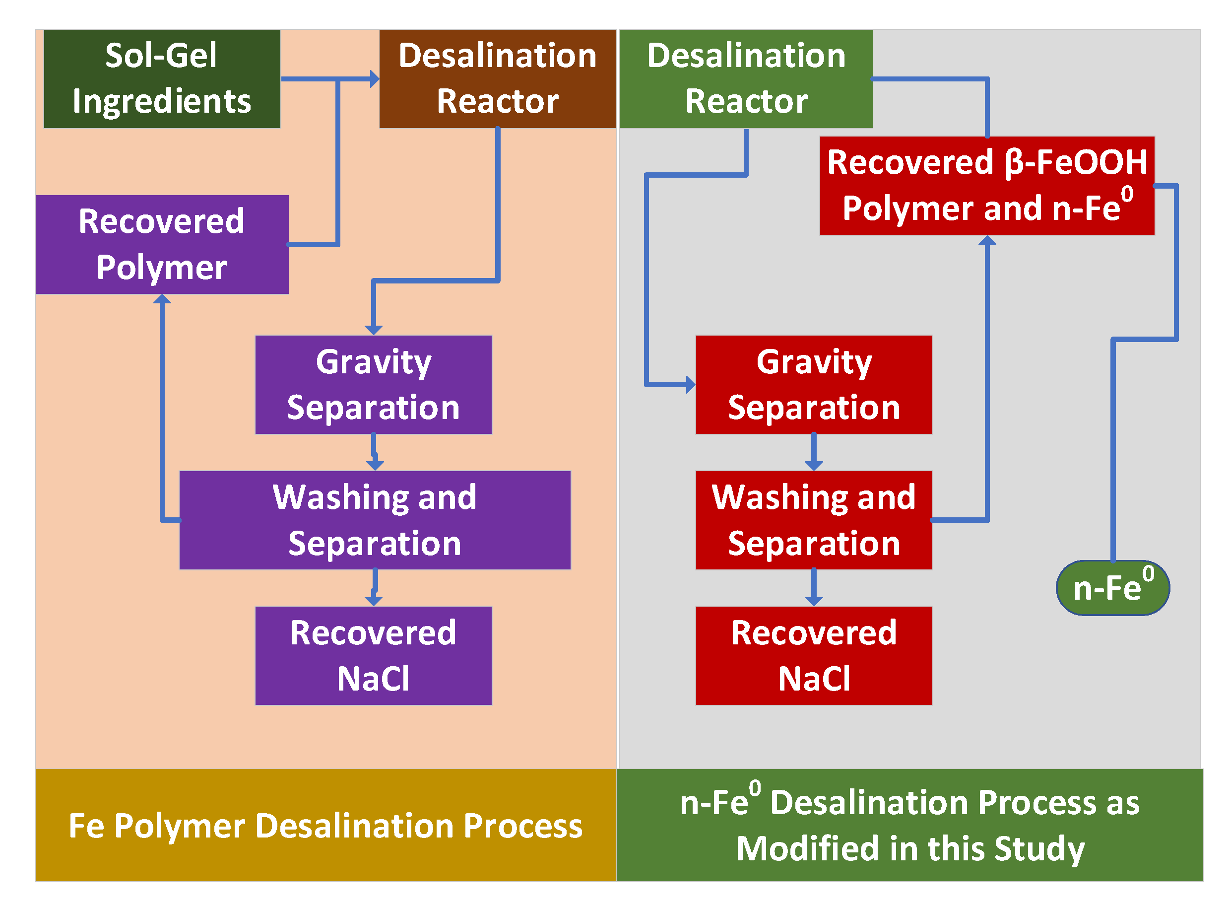
3.10.3. Formation of β-FeOOH and Green Rust Chloride Polymer Spheres

Bare n-Fe⁰ will form, in saline water, an outer coating of β-FeOOH (akageneite) polymers or green rust chloride (Fe(OH)_nCl_y) polymers, commonly termed Fe(a) or Fe(b) or Fe(c) polymers.

The akageneite reacts with saline water as follows:

β-FeOOH + H₂O + Na⁺ + Cl^- = [β-FeOOH @[H⁺ + Cl^-]_{Internal Adsorption}]@[Na⁺ + OH^-]_{external surface adsorption},

(22)

This creates an oxyhydroxide, which contains H⁺ ions and Cl^- ions within its internal tunnel structure [73,74,75,76] and Na⁺ ions and OH^- ions around its periphery. It is an effective adsorber of both anionic and cationic species from water. Compact, β-FeOOH, with 100% occupancy of the internal tunnel sites, has a structure of the form: [≡(OH) ……..Cl^-………(HO) ≡], where the akageneite can be defined as: [β-FeOOH[HCl]_0.256], i.e., 1 g Fe removes 0.16 g Cl^-. Hydrated β-FeOOH, takes the form [β-FeOOH, [H₂O]_n]. This structure allows the hydrated β-FeOOH to absorb more than 1 mole of NaCl for each mole of β-FeOOH. A schematic of the initial particle structuring is shown in Figure 10.

3.10.4. Sphere Growth

The particle flocculates are composed of grains with the structure shown in Figure 10. These flocculates grow by accretion around a particle nucleus (e.g., Figure 11), with a gradual conversion of the n-Fe⁰ core to β-FeOOH (Figure 11). At this point, the structure starts to consolidate with a gradual migration of the β-FeOOH core to the margins and the replacement of the core by both H₂O and H₂ (Figure 11). The fluid-filled sphere grows by accretion, capturing [β-Fe₂(OH)₃]⁺, Fe(OH)ⁿ⁺, and FeOH²⁺] ions. Ion accretion may be expected to increase the thickness of the β-FeOOH rim (Figure 11) as the sphere expands in size. This does not happen (Figure 8b); instead, the rim thickness remains constant or slightly decreases as the particle expands (Figure 8b), and the main expansion of the particle size is associated with an increase in the internal fluid volume (Figure 8c,d). Accreted ions are used to expand the size of the polymer rim.

These observations update and modify the earlier observational models for Fe-polymer colloidal sphere formation documented in references [56,59]. Hollow, self-assembly colloidal spheres, constructed from nanocrystallites/particles, are sometimes termed “superballs” [77].

Hollow β-FeOOH polymer spheres have previously been formulated in experiments, where 0.202 g Fe(NO₃)₃·9H₂O + 0.08 g urea + 0.5 mL 1-n-butyl-3-methyl imidazolium tetrafluoroborate ([BMIM][BF₄]) + 25 mL deionized water were mixed by magnetic stirring at a temperature of 160 °C for a period of 5 to 20 min [78]. The sphere forms from the aggregation of lath-shaped β-FeOOH particles. Dissolution of the laths in within the core, accompanied by migration of the dissolved ions and recrystallization on the outer margins of the laths, may create a hollow core using a form of Otswald ripening [78].

3.10.5. Relationship between Sphere Rim Volume, Fluid Volume and Hydration Shell

The data in Figure 12a indicates that a particle with a rim volume of 10 microns³ will have a fluid core after 2 h of about 0.3 microns³. This increases to >10 micron³ after 4000 h. This analysis indicates that 1 cm³ of β-FeOOH polymer, weighing about 4.25 g, containing 2.8 g Fe, has the potential to directly hold by physical adsorption up to 1.2 g NaCl + 2.14 g NaCl in its core + NaCl in its outer hydration shells. Figure 12b indicates that a 250 nm hydration shell contains more than 3 times the rim volume. It is therefore possible for a charge of n-Fe⁰ to remove more than its own weight, as NaCl adsorbed around a β-FeOOH polymer within the hydration shell.

NaCl can be recovered from a β-FeOOH polymer by simply washing the polymer with deionized water to recover the adsorbed chlorides and sodium [76]. This allows the β-FeOOH polymer to be returned to the reactor for reuse as a desalination agent. An example process flow diagram showing how the n-Fe⁰: n- β-FeOOH polymer or n-Fe⁰:Fe(b) polymer may be commercialized to process saline groundwater or saline flowback water into partially desalinated irrigation water is shown in Figure 13.

The key process requirements are:

• a tank, reservoir, or impoundment to hold the saline groundwater or saline flowback water;
• A reactor that receives water from the tank or impoundment plus a charge of [n-Fe⁰ + n-Fe⁰:Fe polymer + n-Fe polymer];
• A gravity separation unit that recovers the [n-Fe⁰ + n-Fe⁰:Fe polymer + n-Fe polymer] and then discharges a product water (partially desalinated irrigation water). Optionally, part of the product water may be recycled;
• The recovered [n-Fe⁰ + n-Fe⁰:Fe polymer + n-Fe polymer] is recycled, with or without additional processing to remove the adsorbed Na⁺ and Cl^- ions.

This process flow (Figure 13) is relatively simple and robust. It also has a relatively low construction and operating cost. It could easily be constructed on an agricultural unit to convert saline groundwater or saline flowback water held in a tank or impoundment into partially desalinated water.

3.11. Desalination Modeling Associated with n-Fe⁰ or a β-FeOOH Polymer or a Fe(b) Polymer

The primary purpose of the ZVI desalination analyses in this study is to determine how much polymer is required to achieve a specific desalination outcome, the time frame required to achieve the desired outcome, and the reactor size required. This study was designed to understand, for a reactor operating at atmospheric pressure (0.1 MPa) at a temperature in the range of 273 to 298 K, the expected reaction kinetics. This, in turn, defined the required catalyst volume and the required reactor dimensions. This study has also considered the catalyst’s design life and its activity with time (Figure 14). This information is required before the economic viability of the studied desalination routes can be considered.

3.11.1. Example Viability Assessment of the n-Fe⁰:Fe(b) Polymer

An experiment utilizing 25 g L⁻¹ of fresh, Fe₃O₄-coated n-Fe⁰ reduced the water salinity by 15% during the first reaction hour (Figure 8a). The main decline in salinity (Figure 8a) occurred later. The observed relationship (Figure 8a) between Ln(C_{t = n}/C_{t = 0}) versus time, after a reaction time of 100 h (Figure 8a), approximates to:

(C_{t = n}/C_{t = 0}) = e^−0.0116[a] ^−0.3128,

(23)

[a] = water residence time in the reactor, days. C_{t = n} = water salinity at time [a]; C_{t = 0} = initial water salinity. This relationship will differ with the water source and the type of n-Fe⁰ used, but it provides the kinetic data required to size a reactor (Figure 14).

Example Reactor Size Assessment

If a reactor (Figure 13) is to produce 100 m³ d⁻¹ of partially desalinated water using n-Fe⁰ or n-Fe polymer, then, from Figure 8:

• The feed water equates to 4.17 m³ h⁻¹;
• The n-Fe⁰ feed equates to 104.25 kg h⁻¹ (25 g L⁻¹);
• The required desalination in the initial hour is 15% (C_{t = 1h}/C_{t = 0} = 0.85);
• The required reactor volume is 4.17 m³.

1. 

Example Reactor Specification

A suitable reactor (medium density polyethylene, or MDPE) tank (Figure 13 and Figure 14) has dimensions of 2.6 m in diameter; 1.3 m height; 0.14 t of weight; 5 m³ of capacity, 0.62 m access hatch, with ball valve level control, level monitors, and lifting lugs. A typical FOB cost is <USD 1500 (www.directwatertanks.co.uk, accessed on 18 October 2022).

2. 

Example Reactor Operation: Without Recycle

If the reactor is operated without recycle, and with a residence time, t_r, in the reactor of 1 h, then the expected value of (C_{t = n}/C_{t = 0}), from Figure 8, without recycle is about 0.85. The presence, and use, of a recycle loop (Figure 13) will require either the feedwater inflow rate to be decreased or the reactor size to be increased.

3. 

Example Reactor Operation: With Recycle

Recycling 90% of the product water (Figure 13) will require the reactor tank capacity to be increased to about 45 m³. This will require the compact MDPE reactor (Figure 13) to be replaced with a galvanized steel reactor with the following dimensions: 4.6 m diameter; 3.04 m height; capacity 50 m³; EPPM (ethylene propylene diene monomer) liner; 10 cm diameter inlet and outlet pipes; steel cover. A typical FOB, pre-siteworks cost; the pre-installation cost is <USD 5000 (www.directwatertanks.co.uk, accessed on 18 October 2022).

4. 

Example Reactor Operation: With Recycle—Economies of Scale

Increasing the reactor capacity to 500 m³ will require a galvanized steel reactor with dimensions: 12.9 m in diameter; 3.84 m in height; capacity of 500 m³; EPPM (ethylene propylene diene monomer) liner; 10 cm diameter inlet and outlet pipes; steel cover. A typical FOB, pre-siteworks cost; the pre-installation cost is <USD 25,000 (www.directwatertanks.co.uk, accessed on 18 October 2022).

This brief costing analysis indicates that substantial economies of scale may be available as the reactor capacity is increased, with <5-fold increase in I costs for each 10-fold increase in reactor capacity.

Assessing Expected Yield

If 100% of the n-Fe⁰ + β-FeOOH polymer + n-Fe(b) polymer is recovered for recycling (Figure 13), and 90% of the product water is recycled (Figure 13), then:

Ln(C_{t = n}/C_{t = 0})_kinetic = −[a] [a_s] [P_w],

(24)

a_s = particle surface area, m² g⁻¹ = 20 m² g⁻¹ for 50 nm Fe⁰; P_w = particle concentration, g L⁻¹; [a] = normalized rate constant. In Figure 11, the following applies:

Ln(0.85) = −[a],

(25)

In a recycle reactor, where both water and ZVI are recycled (Figure 13), [a] and [a_s] remain constant, but [P_w] increases with time.

Ln(0.85) = −0.16252 = −[a] = [−0.00033],

(26)

This relationship indicates that at t = 1 h, when P_w = 3 g L⁻¹, (C_{t = n}/C_{t = 0}) = 0.98. This is consistent with the observations in Figure 8b,c. This kinetic relationship indicates that if 100% of the n-Fe⁰ + β-FeOOH polymer is recovered for recycling, then P_w and (C_{t = n}/C_{t = 0}) must increase with time while n-Fe⁰ is being added. There will be a loss of activity as some active sites will become blocked during the recycling and regeneration processes (Figure 14), where:

Ln(C_{t = n}/C_{t = 0}) = ([a] [a_s] [P_w])/[d],

(27)

where [d] = site blocking constant where 1 < [d]. [d] will not be known prior to a pilot (or full-scale reactor train) being commissioned, as it is a function of how the feed water interacts with the n-Fe⁰ + β-FeOOH polymer. [d] may vary as a function of time spent in the reaction environment [t], e.g., [d]^[t]. This aging (Figure 14) may be modeled as:

(C_{t = n}/C_{t = 0})_observed = [(C_{t = n}/C_{t = 0})_kinetic [d] ]^[t],

(28)

This model will result in (C_{t = n}/C_{t = 0})_observed initially declining with time before increasing. The n-Fe⁰ + β-FeOOH polymer will be replaced, when (C_{t = n}/C_{t = 0})_observed exceeds a critical value. The life expectancy of a n-Fe⁰ + β-FeOOH polymer in a recycle reactor is not known. This study has only tested a single recycling process.

Impact of Adsorption/Reaction Site Blocking on the Particles

The magnitude of [d] defines the particle life expectancy before either regeneration or replacement is required. The expected modeled operation (Figure 14) of the recycle reactor (Figure 13) for different values of [d] can be used to provide an indication of the expected desalination outcome using Fe₃O₄-coated n-Fe⁰. Bare (uncoated) n-Fe⁰ and other coatings on n-Fe⁰ will have different values for [a] and [d]. They may also have a different relationship between [d] and [t].

• Example Reaction Time and Reactor Size

The reaction time (Figure 14) between the feed water entering the reactor and the product water leaving the separator (Figure 13) is assumed to be 1 h. [R_r] = 0.9; fresh n-Fe⁰ equates to 104.25 kg h⁻¹ for 10 h. No new n-Fe⁰ is added after the initial 10 h. In this model, 100% of the n-Fe⁰ is recycled. This equates to a target n-Fe⁰ + β-FeOOH polymer + n-Fe(b) polymer concentration in the recycle reactor (Figure 14) of around 225 g L⁻¹ (Figure 15a).

In this example, where [R_r] = 0.9, the process water volume within the reactor (Figure 13 and Figure 14) stabilizes at about 41 m³ (Figure 15b). This stabilized volume (required reactor size) increases as [R_r] increases above 0.9 but decreases as [R_r] decreases below 0.9. The product water outflow rises to a stable output level, which equals the feed water flow rate (Figure 15c). The time taken to reach this flow rate is a function of the recycle ratio. This stabilization time increases as [R_r] increases.

• Example Product Water Salinity

The product water salinity is a function of [d] (Figure 14 and Figure 15d). Ideally, [d] = 1. In reality, [d] will be >1. The product water salinity reduces to a base level (Figure 15d). This base level is controlled by the amount of n-Fe⁰ + β-FeOOH polymer (P_w = g L⁻¹) within the recycle reactor. The total amount of desalination increases as P_w increases.

This kinetic modeling (Figure 14) indicates that (C_{t = n}/C_{t = 0})_observed is minimized (i.e., desalination is maximized) by maximizing [a] and minimizing [d]. The parameter [d] controls the economic life expectancy of the n-Fe⁰ + β-FeOOH polymer within the reactor (Figure 14) and the economic viability of the desalination process. The parameter [a] controls the minimum achievable value for (C_{t = n}/C_{t = 0})_observed (Figure 14).

The effectiveness of a β-FeOOH polymer decreases with decreasing water salinity and decreases with decreasing water pH. Initially, the n-Fe⁰ is used to increase the water’s pH (Figure 8). Once the addition of fresh n-Fe⁰ to the reactor ceases (Figure 15a), the pH of the water retained in the reactor will gradually decrease (Figure 8), and [d] will increase (Figure 15d).

3.11.2. Significance of Increasing P_w

The modeling in Figure 15d demonstrated that operating the process (Figure 13 and Figure 14) with recycle and an initial n-Fe⁰ charge of 25 g L⁻¹ (for 10 h) with 100% ZVI recycle thereafter, it may be possible to achieve C_{t = n}/C_{t = 0} of 80%, i.e., 20% desalination. Increasing P_w to 50 g L⁻¹ (for 10 h) allows C_{t = n}/C_{t = 0} to reduce to 61% (Figure 15e). Increasing P_w further to 100 g L⁻¹ (for 10 h) allows C_{t = n}/C_{t = 0} to reduce to 38% (Figure 15f), i.e., 62% desalination.

This analysis indicates that the economic viability of partial desalination (Figure 14) using n-Fe⁰:Fe(b) is a function of [a], [d] and P_w. [a] controls the amount of n-Fe⁰ required (P_w), to achieve a specific C_{t = n}/C_{t = 0} ratio. [d] controls the frequency of n-Fe⁰ replacement, and the decline in catalytic efficiency (Figure 14).

For example, if the maximum acceptable C_{t = n}/C_{t = 0} ratio was 0.5, Figure 15d would indicate the following replacement, or regeneration, intervals:

• [d] = 1.02, replacement is at 15-h intervals (processing 62 m³);
• [d] = 1.01, replacement is at 29-h intervals (processing 120 m³);
• [d] = 1.005, replacement is at 56-h intervals (processing 233 m³).

These parameters are specific to a specific batch and composition of n-Fe⁰, a specific water composition, a specific reactor process, and a specific mode of reactor operation. They may also vary with temperature. Replacing Fe₃O₄ coated n-Fe⁰ with uncoated n-Fe⁰ will increase [a], possibly by several orders of magnitude. This increase in [a] will be accompanied by an increase in [d], requiring more frequent replacement of the n-Fe⁰, but the increase in [a] may allow P_w to be reduced.

This analysis indicates that if the n-Fe⁰ recovery system is switched from magnetic separation to gravity separation, and if it is assumed that the primary agent for ion removal is n-Fe⁰:Fe polymers, then it may be possible to substantially reduce the cost of using n-Fe⁰ to produce partially desalinated irrigation water from groundwater.

4. Boosting Desalination Using Sol-Gel Polymers

The preceding analysis has indicated that n-Fe⁰ can be used to provide a source of β-FeOOH polymer, or Fe(a), Fe(b), and Fe(c) polymer in the water. The principal expenses associated with the process are: (i) the cost of n-Fe⁰; (ii) the large tank sizes associated with the slow reaction rates, and the requirement for a high recycle ratio.

This study has identified that the principal desalination agent may not be n-Fe⁰, but is instead a derivative polymer (Fe(a,b,c)). The formation of these derivative polymers allows the desalination reaction to proceed. These polymers have not been specifically identified, but the redox environment is consistent with the presence of akaganeite (β-FeOOH polymer), other FeOOH polymers, and green rust (Fe_xO_yH_z) polymers. These polymers and associated ions can be formed directly from Fe⁰, e.g., [52],

Fe0 + H2O = HFeOHx+,

(29)

Increasing the rate at which n-Fe⁰ produces polymeric ions (e.g., –[HFeOH^x+]^n-) will increase the desalination rate and reduce the P_w required to achieve a specific desalination rate. Substituting Fe⁰ with Feⁿ⁺ may make it possible to manufacture n-[β-FeOOH polymer] or an equivalent polymer within the reactor, using a substantially smaller quantity of Fe.

Since the materials required to manufacture Feⁿ⁺ ions are perhaps two to four orders of magnitude cheaper to purchase than n-Fe⁰, are widely available, and are safer to handle than n-Fe⁰, it may be more effective to manufacture the Fe-polymers directly from dissolved ions within the reactor, using a sol-gel approach, rather than from n-Fe⁰.

This concept is summarized in Figure 16. This section investigates whether the sol-gel approach may provide a viable route that could allow saline groundwater to provide partially desalinated irrigation water for a cost of <USD 0.5 m⁻³.

4.1. Reactor Process Flow

The initial n-Fe⁰ process flow assumed that Fe-polymers (iron corrosion products) formed no part of the desalination process (Appendix A). Desalination was undertaken by functionalized magnetic n-Fe⁰ (Appendix A). The experimental observations that iron polymers are directly associated with desalination [6] or catalyze desalination [4,7], provided the technical basis for the revisiting of this hypothesis. The experimental data in Figure 8b,c demonstrated that higher desalination rates occur in the reused non-magnetic n-Fe⁰:Fe(b) polymer.

This suggests that many of the operational issues associated with operating a reactor with functionalized magnetic n-Fe⁰ are over complications and that the process could be simplified by replacing the magnetic separators with a simple gravitational separator (Figure 13). This then allows the non-magnetic n-Fe⁰:Fe(b) polymer to be washed to recover bound NaCl prior to reuse (Figure 13). This process restructuring creates an obvious reduction in both processing costs and material requirements in desalinating saline groundwater to produce partially desalinated irrigation water, relative to the prior art (Appendix A).

The principal material cost in the revised n-Fe⁰:Fe(b) polymer desalination process is the cost of the n-Fe⁰. The revised n-Fe⁰:Fe(b) polymer model indicates that the sole function of the n-Fe⁰ is to act as a generating source of Fe(b) polymers. This conclusion is consistent with the operating results of a catalytic pressure swing adsorption/desorption desalination reactor [7], which demonstrated that supported Fe(b) polymers could catalyze the formation of entrained hydrated Fe(b) polymers within the water body. These entrained polymers desalinated the water. A follow-up series of experiments [59] established that sol-gel polymers may have the potential to replace n-Fe⁰ and n-Fe⁰:Fe(b) polymers.

The key feature associated with n-[β-FeOOH polymer] formation associated with n-Fe⁰ is the increase in pH into the range of 8 to 11 (Figure 8). This is associated with the availability of Feⁿ⁺ ions, produced from the corrosion of n-Fe⁰. The sol-gel precipitates used in this study are designed to increase the product water’s pH into the range of 9 to 13.

4.2. Increasing pH to Facilitate Sol-Gel Formation

Adding CaO (or a soluble carbonate) to water increases its pH. Therefore, addition to water of CaO (or another oxide (ZnO), or a soluble bicarbonate/carbonate) to saline water containing Feⁿ⁺ ions will result in the precipitation of β-FeOOH polymer, Fe polymers, and green rust polymers [59]. The addition of Feⁿ⁺ ions to water containing organic species, such as acids or polyphenols, will also result in the precipitation of n-Fe@organic polymer species [56,59]. The target Eh:pH regime for the sol-gel polymer formation is summarized in Figure 3.

4.3. Fe-Ca Polymer

Ion removal for both Cl^- and Na⁺ ions approximate to a relationship of the form [59]:

(C_{t= n}/C_{t =0}) = exp(−(([a] [a_s]) [P_w])[t_r][b])(3600 t_r)),

(30)

where ([a] [a_s] [P_w]) and [b] are derived from a regression plot of Ln(C_{t = n}/C_{t = 0}) versus residence time, [t_r], hours (

Table 1. Fe-Ca polymer.; R² = Coefficient of determination; PCC = Pearson’s Correlation Coefficient. All weights are g L⁻¹. Data Source: Table A5 reference [20]. Trial 1. 1.4 g FeSO₄ + 3.34 g CaO; feed water salinity (FW): = 14.38 g NaCl L⁻¹; Trial 2. 1.4 g FeSO₄ + 1.67 g CaO; FW = 15.27 g NaCl L⁻¹; Trial 3. 1.4 g FeSO₄ + 3.34 g CaO + 1.32 g urea; FW = 30.14 g Cl^- L⁻¹ + 18.38 g Na⁺ L⁻¹; Trial 4. 1 g FeSO₄ + 1.67 g CaO + 2.52 g MnO₂ + 1 cm³ formic acid; FW = 30.14 g Cl^- L⁻¹ + 18.38 g Na⁺ L⁻¹; Trial 5. 1 g FeSO₄ + 3.34 g CaO + 2.52 g MnO₂ + 1 cm³ formic acid; FW = 30.14 g Cl^- L⁻¹ + 18.38 g Na⁺ L⁻¹; Trial 6. 0.8 g FeSO₄ + 3.34 g CaO + 2.71 g ZnO + 0.94 g gallic acid; FW = 22.11 g Cl^- L⁻¹ + 14.33 g Na⁺ L⁻¹; Trial 7. 1.42 g FeSO₄ + 5.61 g ZnO; FW = 30.47 g Cl^- L⁻¹ + 10.3 g Na⁺ L⁻¹. Trial 8. 1.0 g FeSO₄ + 1.67 g CaO + 2.52 g MnO₂ + 2.96 g MgCO₃ + 1 cm³ formic acid; FW = 26.55 g Cl^- L⁻¹ + 17.21 g Na⁺ L⁻¹ Trial 9. 1 g FeSO₄ + 3.34 g CaO + 2.52 g MnO₂ + 1 cm³ formic acid; FW = 22.11 g Cl^- L⁻¹ + 14.33 g Na⁺ L⁻¹; Trial 10. 2.0 g FeSO₄ + 3.34 g CaO + 11.22 g ZnO + 0.9 g tartaric acid; FW = 23.22 g Cl^- L⁻¹ + 19.83 g Na⁺ L⁻¹.

		Cl-				Na+
Polymer	Trial	[a]	[b]	R2	PCC	[a]	[b]	R2	PCC
Fe-Ca	1	0.000120540	−0.9842	0.999	1.000	0.0000851	−0.92801	0.997	0.998
	2	0.000168210	−0.9867	0.999	0.999	0.0000039	−1.61133	1.000	1.000
Fe-Ca-Urea	3	0.000278500	−0.9542	0.954	0.977	0.0001331	−1.01025	1.000	1.000
Fe-Ca-Mn-Formic Acid	4	0.000049800	−0.4236	0.918	0.958	0.0002348	−1.05551	0.842	0.918
	5	0.000135500	−0.7804	0.975	0.987	0.0002164	−0.88604	0.955	0.977
Fe-Ca-Zn-Gallic Acid	6	0.000020820	−0.5451	1.000	1.000	14.4647000	−0.00100	1.000	1.000
Fe-Zn	7	0.000027580	−1.1817	1.000	1.000	0.0000730	−0.86425	0.999	0.999
Fe-Ca-Mn-Mg-Formic Acid	8	0.000179580	−0.7637	0.990	0.995	0.0001411	−0.94756	0.996	0.998
Fe-Ca-Mn-Formic Acid	9	0.000031490	−0.4312	0.732	0.856	0.0001519	−0.92883	0.906	0.952
Fe-Ca-Zn- Tartaric Acid	10	0.000289940	−0.7276	0.963	0.981	0.0003781	−0.86185	0.988	0.994

). This sol-gel combination has an expected low level of Na⁺ removal (<5%) combined with 35–45% Cl^- ion removal after an hour. The expected relationships between (C_{t = n}/C_{t = 0}) and t_r are provided in Figure 17. The amount of desalination increases with increasing P_w and decreases with t_r as [d] increases. The cationic nature of this polymer is consistent with the formation of a β-FeOOH polymer.

4.4. Fe-Ca-Urea Polymer

Replacing n-Fe⁰ with a Fe-Ca-urea and sol-gel combination (Table 1) indicates an expected 38% Na⁺ removal combined with a 63% Cl^- ion removal after an hour. Replacing the 25 g of n-Fe⁰ L⁻¹ with this polymer (1.4 g FeSO₄ L⁻¹) in the recycle reactor increases the polymer’s life (Figure 17c) when compared to the n-Fe⁰ + β-FeOOH polymer (Figure 15d). The addition of urea adds both cationic and anionic sites to the polymer.

4.5. Fe-Ca-Mn-Formic Acid Polymer

Replacing n-Fe⁰ with a Fe-Ca-Mn-Formic acid sol gel combination (Table 1) indicates an expected 54–58% Na⁺ removal combined with a 17–39% Cl^- ion removal after an hour. Replacing the 25 g of n-Fe⁰ L⁻¹ with this polymer (1 g FeSO₄ L⁻¹) in the recycle reactor increases the polymer’s life (Figure 17d,e), when compared to the n-Fe⁰ + β-FeOOH polymer (Figure 15d).

4.6. Fe-Ca-Zn-Galic Acid Polymer

Replacing n-Fe⁰ with a Fe-Ca-Zn-gallic acid sol-gel combination (Table 1) indicates an expected 0% Na⁺ removal combined with a 7% Cl^- ion removal after an hour. Increasing the amount of FeSO₄ from 0.8 g L⁻¹ to 8 g L⁻¹ increases, after 1 h, the Na⁺ removal to 1% and the Cl^- removal to 52%. Replacing the 25 g of n-Fe⁰ L⁻¹ with this polymer (8 g FeSO₄ L⁻¹) in the recycle reactor increases the polymer life (Figure 17f), when compared to the n-Fe⁰ + β-FeOOH polymer (Figure 15d). This polymer initially preferentially removes Cl^- ions before removing Na⁺ ions. This is consistent with the initial Fe@gallic acid polymer being dominated by cationic sites.

4.7. Fe-Zn Polymer

Replacing n-Fe⁰ with a Fe-Zn sol gel combination (Table 1) indicates an expected 23% Na⁺ removal combined with a 9% Cl^- ion removal after an hour. Increasing the amount of FeSO₄ from 1.42 g L⁻¹ to 14.2 g L⁻¹ increases, after 1 h, the Na⁺ removal to 92% and the Cl^- removal to 62%. Replacing the 25 g n-Fe⁰ L⁻¹ with this polymer (14.2 g of FeSO₄ L⁻¹) in the recycle reactor increases the polymer’s life (Figure 17g), when compared to the n-Fe⁰ + β-FeOOH polymer (Figure 15d). This polymer contains a higher proportion of anionic sites relative to cationic sites.

4.8. Fe-Ca-Mn-Mg-Formic Acid Polymer

Replacing n-Fe⁰ with a Fe-Ca-Mn-Mg-formic acid sol gel combination (Table 1) indicates an expected 40% Na⁺ removal combined with a 48% Cl^- ion removal after an hour. Replacing the 25 g of n-Fe⁰ L⁻¹ with this polymer in the recycle reactor increases the polymer’s life (Figure 17h), when compared to the n-Fe⁰ + β-FeOOH polymer (Figure 15d). This polymer has a similar proportion of cationic and anionic sites.

4.9. Fe-Ca-Mn-K-Formic Acid Polymer

Replacing n-Fe⁰ with a Fe-Ca-Mn-K-formic sol gel combination (Table 1) indicates an expected 75% Na⁺ removal combined with a 65% Cl^- ion removal after an hour. Replacing the 25 g n-Fe⁰ L⁻¹ with this polymer in the recycle reactor increases the polymer’s life (Figure 17i), when compared to the n-Fe⁰ + β-FeOOH polymer (Figure 15d).

4.10. Fe-Ca-Zn-Tartaric Acid Polymer

Replacing n-Fe⁰ with a Fe-Ca-Zn-tartaric acid sol gel combination (Table 1) indicates an expected 74% Na⁺ removal combined with a 64% Cl^- ion removal after an hour. Replacing the 25 g n-Fe⁰ L⁻¹ with this polymer in the recycle reactor increases the polymer’s life (Figure 17j) when compared to the n-Fe⁰ + β-FeOOH polymer (Figure 15d). This polymer contains a similar proportion of cationic and anionic sites.

5. Expected Desalination

The amount of desalination that could be achieved in a recycle reactor (Figure 13), for a specific R_r, is a function of the average P_w, and [d] (Figure 14). Any commercial application of this technology for the treatment of groundwater will require the following criteria (Figure 2) to be met:

• The technology should be able to partially desalinate the irrigation water;
• The pH of the irrigation water and composition of the residual polymers and ions in the water should not adversely affect either the plant (crop) growth or the soil structure;
• The technology should improve the standard measures used by the regulatory agricultural authorities to assess the suitability of water for irrigation;
• The amount of desalination achieved should be sufficient to induce an increase in crop yield (t ha⁻¹), without inducing a decrease in crop value (USD t⁻¹);
• Application of the partially desalinated irrigation water should decrease soil salinization and should not contribute to soil salinization. Increasing soil salinization is associated with decreasing agricultural land values (USD ha⁻¹);
• The cost of providing the partially desalinated irrigation water should be less than the increased net revenue resulting from increased crop yields associated with using the water;
• The regulatory authorities provide approval for the use of the appropriate desalination polymer, provide approval for irrigation overland flow to enter the local riparian environment, and provide approval for the resultant soil throughflow to enter both the shallow groundwater environment and the local riparian environment, through field drainage to ditches and streams, etc.

5.1. Environmental Impact

The use of n-Fe⁰ in treating groundwater within aquifers is subject to regulation in many countries. The use of most chemicals for application to the soil, where there is a risk that the chemicals could either reach groundwater or the riparian environment or potentially interfere with potable water supplies, is also subject to regulation in many countries.

In this study, the polymer ingredients were selected from widely available agricultural chemicals. This was to reduce the risk that the chemicals associated with the partially desalinated water would have an adverse impact on plant growth and also to reduce the risk that the regulatory authorities would place impractical requirements on their use to create partially desalinated irrigation water from saline groundwater.

All the chemicals used to form the polymers are used as fertilizers for some agricultural applications: ZnO [79]; CaO [80,81]; MnO₂ [82,83]; Fe_SO₄ [84,85]; MgCO₃ [86,87]; K₂CO₃ [88]; formic acid [89]; tartaric acid [90]; and urea [91,92]. Therefore, excess quantities of these components in the desalinated water are likely to assist crop growth.

5.2. Indicative Costs

If the polymer ingredients for a reactor charge cost USD y, then:

Cost (USD m⁻³) = (y × t_n/10)/(t_nP_r)

(31)

t_n = number of hours (h) of processing using a single polymer charge; P_r = partially desalinated water production rate, m³ h⁻¹. The choice of polymer, and t_n is a function of the feed water composition, required level of desalination. Example polymer costs are provided in

Table 2. Example costs. Material costs are FOB, USD t⁻¹, Source—(www.alibaba.com, accessed on 5 October 2022); Polymer A = 2.0 g FeSO₄ L⁻¹ + 3.34 g CaO L⁻¹ + 11.22 g ZnO L⁻¹ + 0.9 g Tartaric Acid L⁻¹; Polymer B = 1.4 g FeSO₄ L⁻¹ + 3.34 g CaO L⁻¹ + 1.32 g Urea L⁻¹. Polymer A and B ingredient costs (FOB) are USD m⁻³ processed (without polymer recycle).

	FeSO4	CaO	ZnO	Tartaric Acid	Urea	Polymer A	Polymer B
Low	80	60	2900	1500	15	34.25	0.33
High	150	120	3200	30,000	150	63.60	0.81

.

These two example polymers provide an example of the material cost. For the purposes of this study, an of example saline flowback water from the Marcellus Shale (

Table 3. Example flowback water composition from a shale gas well, USA (Marcellus Shale). All measurements are in g L⁻¹. EC1 = EC when F = 0.55; EC2 = EC when F = 0.7. EC units = dSm⁻¹ (mScm⁻¹); FeSO₄ data is excluded from the compositional analysis and the EC calculations. EC and SAR calculations assume that the Ca remains in solution and is not incorporated in the Fe(a,b,c) polymers. Incorporation of Ca in the polymers will result in a lower EC and a higher SAR.

	Ca	K	Mg	Na	Cl	HCO3	SO4	NaCl	SAR	EC1	EC2
Example Well	0.1633	0.0327	0.0262	4.659	7.64	1.036	0.0656	12.3	125.94	24.77	19.46
0% Desalination	2.5490	0.0327	0.0262	4.659	7.64	1.036	0.0656	12.3	35.58	29.11	22.87
20% Desalination	2.5490	0.0327	0.0262	3.727	6.11	1.036	0.0656	9.8	28.47	24.63	19.36
50% Desalination	2.5490	0.0327	0.0262	2.330	3.82	1.036	0.0656	6.1	17.79	17.93	14.08
80% Desalination	2.5490	0.0327	0.0262	0.932	1.53	1.036	0.0656	2.5	7.12	11.22	8.81
100% Desalination	2.5490	0.0327	0.0262	0.000	0.00	1.036	0.0656	0.0	0.00	6.74	5.30

) is used to illustrate the possible outcomes associated with using the Fe-Ca-Urea polymer (Polymer B, Table 2). The data source for this water composition is [59]. The target salinity (Figure 14) is between 1 and 2 g NaCl L⁻¹.

5.3. Regulatory Indices

Regulatory consent procedures and requirements vary between countries. Regulatory consent (Figure 2) to use desalinated irrigation water commonly requires that the irrigation water comply with regulation-defined criteria and compositional indices. Examples of appropriate compositional indices are provided in Appendix C. The most widely considered regulatory criteria for the characterization of irrigation water (apart from electrical conductivity (EC)) is the sodium adsorption ratio (SAR) [41] (Appendix C). The exact values of SAR that are acceptable to a regulatory authority vary globally. The Fe@Ca polymers decrease Na⁺ while increasing Ca²⁺. This has the effect (Appendix C) of reducing SAR as the salinity decreases (Table 3). FAO guidelines recommend regulatory restrictions on irrigation water use when EC > 3 dSm⁻¹ and SAR >3.0. The analysis in Table 3 indicates that the product water EC will be >3 unless measures are adopted to remove Fe-Ca polymers following processing. Their removal from the product water in a gravitational separator (Figure 13) will allow the product water to potentially have EC < 3 dSm⁻¹ and SAR <3.0.

5.4. Example Fe-Ca-Urea Polymer Analysis

The Fe-Ca-urea polymer’s effectiveness is a function of P_w and [d] (Figure 18). The data in Table 3, indicates that the required C_{t = n}/C_{t = 0} should be <16%, to achieve a salinity of <2 g L⁻¹. Modeling (Figure 18) using the data set in Table 2 indicates that this criterion is met, when P_w includes >5.6 g FeSO₄ L⁻¹ (Figure 18d).

Increasing the level of Ca²⁺ ions will assist in reducing the SAR value (Appendix C) into the range 1.83 to 3.67, if the salinity can be reduced into the range of 1.2 to 2.5 g L⁻¹ (

Table 4. Example flowback water composition from a shale gas well, USA (Marcellus Shale), where P_w includes >5.6 g FeSO₄ L⁻¹. All measurements are in g L⁻¹. EC1 = EC, when F = 0.55; EC2 = EC, when F = 0.7. EC units = dSm⁻¹ (mScm⁻¹); FeSO₄ data is excluded from the compositional analysis. Product water composition entering the gravitational separator.

	Ca	K	Mg	Na	Cl	HCO3	SO4	NaCl	SAR	EC1	EC2
Example Well	0.1633	0.0327	0.0262	4.659	7.64	1.036	0.0656	12.3	125.94	24.77	19.46
0% Desalination	9.7062	0.0327	0.0262	4.659	7.64	1.036	0.0656	12.3	18.35	42.12	33.09
20% Desalination	9.7062	0.0327	0.0262	3.727	6.11	1.036	0.0656	9.8	14.68	37.65	29.58
50% Desalination	9.7062	0.0327	0.0262	2.330	3.82	1.036	0.0656	6.1	9.17	30.94	24.31
80% Desalination	9.7062	0.0327	0.0262	0.932	1.53	1.036	0.0656	2.5	3.67	24.23	19.04
90% Desalination	9.7062	0.0327	0.0262	0.466	0.76	1.036	0.0656	1.2	1.83	21.99	17.28
100% Desalination	9.7062	0.0327	0.0262	0.000	0.00	1.036	0.0656	0.0	0.00	19.76	15.52

). The modeled data indicates (Figure 18) that this may occur if P_w includes >5.6 g FeSO₄ L⁻¹ (Figure 18d).

The efficiency of the gravitational separator will define both the SAR value and the EC of the product water. Table 4 indicates the expected water compositions without removal of the polymer precipitate from the water. Removal of the polymer precipitate will reduce the product irrigation water’s EC and SAR.

Example Impact of Polymer Recycle on Product Water Composition

If the reactor (Figure 13) is filled with 4.17 m³ of saline water plus 22.96 kg FeSO₄ + 54.78 kg CaO + 21.65 kg urea (Figure 18d, Table 4), and the reactors’ (Figure 13 and Figure 14) operating conditions are:

• Feed water flow rate = 4.17 m³ h⁻¹;
• Product water flow rate = 4.17 m³ h⁻¹;
• R_r = 0% for product water; R_r = 100% for polymer recovered from the separator;
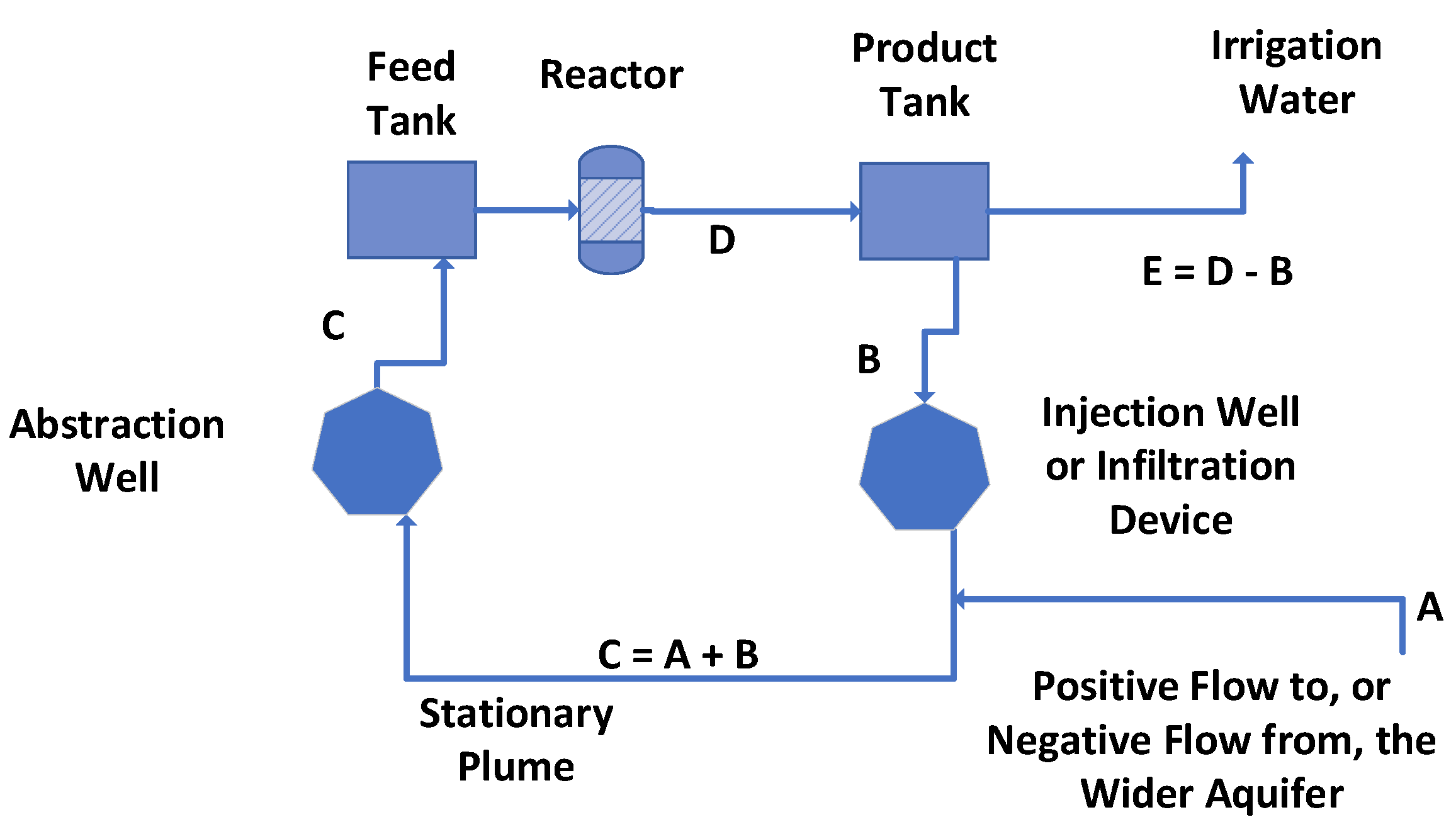
• Reactor volume = 4.17 m³, including flowlines to the separator (Figure 17).
• t_r = 1 h;
• [d] is between 1.005 and 1.01.

Then, the expected product water salinity will be <2 g NaCl L⁻¹ for between 90 h ([d]= 1.01) and 185 h ([d]= 1.005), i.e., a single catalyst (sol-gel polymer) charge costing about USD 3.33 will process between 375 and 770 m³ (Figure 19a,b). Reactivation of the polymer is achieved by washing it in fresh water. This reduces the net polymer cost for the water processing to between USD 0.0044 and 0.0088 m⁻³.

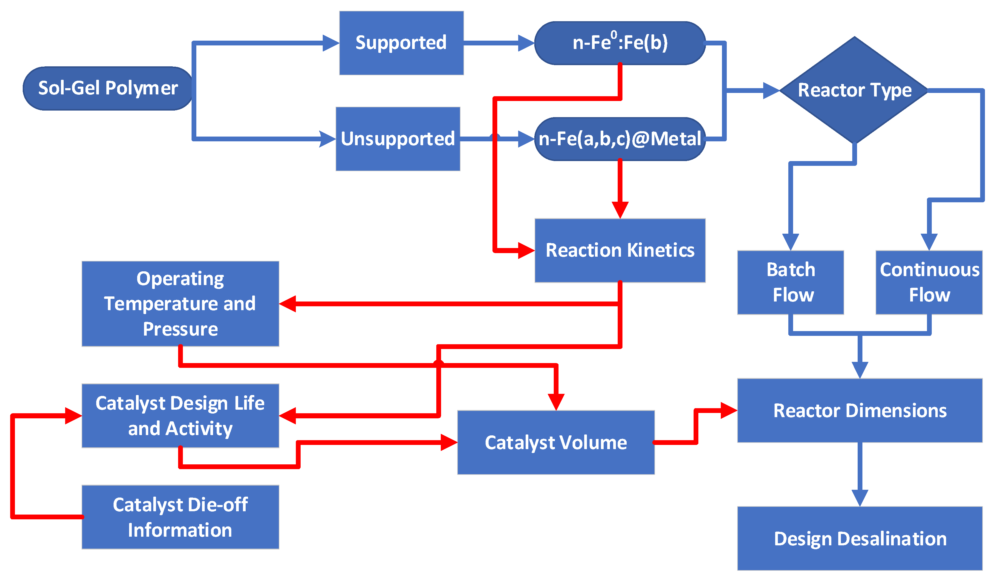
6. Application to Groundwater Management

The discussion and analysis in Section 3, Section 4 and Section 5 have focused on:

• Reaction kinetics (Figure 14) considering:

  ∘

  Polymer Type

  ■

  Supported: n-Fe⁰:Fe(b);

  ■

  Unsupported: n-Fe(b);

  ∘

  Static diffusion operating conditions;

  ∘

  Pressure of 0.1 MPa and temperature of 273–298 K;

  ∘

  Different P_w;

  ∘

  Different activity dieback relationships;

• Reactor Operation (Figure 13) considering:

  ∘

  desalination with no product water recycled to the reactor;

  ∘

  desalination with product water recycled to the reactor;

  ∘

  desalination with polymer recycled to the reactor.

This analysis has established that the polymer desalination process may provide a technically viable solution for the provision of irrigation water from groundwater or flowback water. This product water will either be placed in storage for later use or be used as it is produced. Storage can be:

• Above ground in tanks or impoundments. This is the conventional approach. The typical irrigation requirement is 1000–10,000 m³ ha⁻¹ a⁻¹. An agricultural holding of 100 ha, would require surface-based storage (e.g., 3 m deep) covering 33,000–330,000 m² (3.3 to 33 ha). This large land take for desalinated water storage may be both physically and economically impractical.
• In the subsurface, contained within hydrodynamic mounds or plumes. The latter approach allows the reactor (Figure 13) to be used to desalinate part of an aquifer or soil body (Figure 2 and Figure 20).

The desalinated water created using this process (Figure 2) can be used to reconstruct the groundwater in three areas: (i) the creation of stationary hydrodynamic plumes of desalinated water within saline aquifers; (ii) the creation of shallow pressured mounds (containing desalinated water) within salinized impermeable soils; and (iii) the prevention, stabilization, and reversal of seawater intrusion within an aquifer. The decision process flow used to achieve this is summarized in Figure 20. A more detailed analysis of this process, which demonstrates the potential applications of the polymers for sub-surface storage and for desalinating aquifers and soils, is provided in Appendix D.

7. Commerciality

ZVI desalination technology is at various stages of commerciality. Desalination processes based on n-Fe⁰ have undergone pre-commercial (commercial scale) trials (since 2014) in the USA, tackling waste saline water associated with hydrocarbon extraction and mine waters. The desalination processes based on Fe⁰:Fe(b)@urea polymers and SiO₂@Fe(b)@urea polymers [4,7] have undergone pre-commercial (commercial scale) trials in the UK (since 2015).

This study has focused on a static diffusion and batch flow analysis in order to determine whether this polymer process may provide an alternative route to commerciality. Batch flow trials can be used to design both batch flow reactors and continuous flow reactors. Historically, multi-tubular reactor design and commerciality decisions have normally focused on the performance of a single commercial-scale tube.

The kinetic results (Table 2) established that the catalyst’s effectiveness increases with residence time within the reactor. It had previously been established [93] that the coagulation rate to form polymeric agglomerates increases as:

• The turbulence within the reaction environment increases; and
• The pH in the turbulent environment increased.

The increase in rate constant resulting from a combination of a pH increase and turbulence can be several orders of magnitude [93].

The majority of polymeric catalysts examined in Table 2 resulted in the pH of the product water being higher than the pH of the feed water. n-Fe@Ca@gallic acid polymers (e.g., Trial 6, Table 2; Figure 17f) operate by first reducing the pH (due to the presence of gallic acid and SO₄^2- ions). The pH then slowly rises as the CaO gradually forms Ca(OH)₂. The final pH of the product water can be the same as or similar to the pH of the feed water. An example analysis, processing 240 L of seawater, is shown in Figure 21. This analysis (Figure 21d), when compared with the 2.3 L kinetic data (Figure 17f), indicates that in the 240 L reactor, [d] >1.01.

An initial program of pre-commercial (commercial scale) desalination trials using these polymers, based on a multi-tubular, transport line reactor design, has been commenced. Preliminary results using n-Fe@Ca@Zn@gallic acid polymers at a continuous flow rate of 24 L h⁻¹, through a 3 m long, 0.042 m O.D. uni-tubular reactor (reaction time = 3.14 min) have achieved an average Cl^- removal of 63% and an average Na⁺ ion removal of 38%, from feed water with an average salinity of 11.68 g L⁻¹ (feed water pH = 9.1; product water pH = 10.3; polymer composition: Table 2: Trial 6; continuous run time = 10 h). These observations (when compared with Figure 21) confirm that an increase in the desalination rate constant can be achieved in a transport line reactor from a combination of a rapid pH increase and a turbulent reaction environment, and that the associated increase in the rate constant can be several orders of magnitude when compared with a batch flow example (Figure 17f and Figure 21).

The formation of stationary hydrodynamic plumes and groundwater mounds has been demonstrated in both aquifers and soils (Appendix D). The future field groundwater tests, which adopt the process decision flow shown in Figure 2 and Figure 20, are contingent on the results of both commercial-scale polymer trials and the identification of suitable application areas.

8. Conclusions

Five different groups of ZVI-based partial desalination routes have been compared (n-Fe⁰; n-Fe₃O₄; Fe⁰:Fe(b)@C⁰; n-Fe:Fe(b); n-Fe(b)). These have been subdivided into two basic processing groups based on the mechanism for recovering the ZVI from the product water prior to recycling. These are:

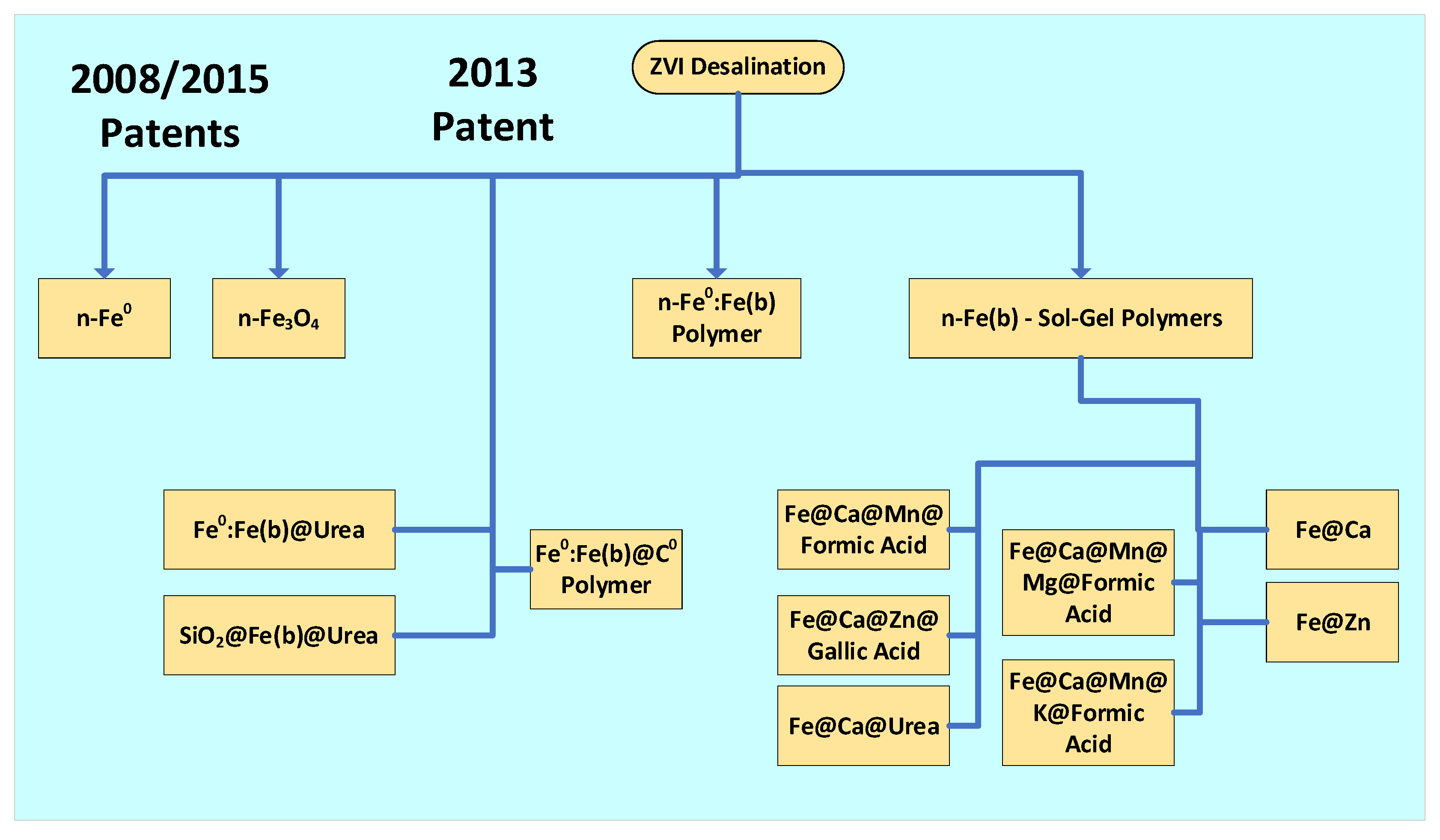
• Magnetic separation route (n-Fe⁰; n-Fe₃O₄);
• Gravitational separation route (Fe⁰:Fe(b)@C⁰; n-Fe:Fe(b), n-Fe(b)).

The analysis concludes that the only potentially economically viable routes (to produce desalinated water for irrigation) involve gravity separation and recycling. The screening analysis indicated that a n-Fe(b) polymer constructed using FeSO₄ + CaO + urea may provide a processing route that could result in 80–90% ion removal in a static diffusion batch flow environment within a 1-h processing time. The examples demonstrate that this route may potentially allow both saline groundwater and flowback water to be desalinated to form partially desalinated irrigation water for a cost of less than USD 0.5 m⁻³.

Batch flow scaleup from a 2.3 L reactor to a 240 L reactor processing seawater using an n-Fe(b)@Ca@Zn@gallic acid polymers demonstrated that:

• The kinetic desalination results from a 2.3 L reactor operation are effectively replicated in a 240 L reactor, indicating that it may be reasonable to expect that the desalination results from a 240 L reactor will be replicated in a 24 m³ reactor;
• The site blocking constant [d] was increased to between 1.01 and 1.015, relative to the 2.3 L reactor;
• Desalination increases as pH increases and Eh decreases.

This information indicated that it may be possible to substantially increase the rate constant by switching to a transport line reactor, processing 24 L h⁻¹ tube⁻¹ over 10 h. This reactor incorporated a rapid pH shift combined with a turbulent environment. This was demonstrated to reduce the time taken to achieve an average Cl^- removal of 63% and an average Na⁺ ion removal of 38% (average 50.5% desalination) from between 23 h (2.3 L reactor) and 120 h (240 L reactor) to 3.14 min. The operation in a transport line reactor reduced [d] to below the normalized value of [1] in the 2.3 L reactor.

These observations suggest that static diffusion reactor scale-up results in an increase in [d], while switching from a static diffusion reactor to a transport line reactor results in a substantial decrease in [d].

A combination of hydrodynamic and adsorption/catalytic modeling has established that a commercial-scale reactor scale-up could be used to desalinate part of a confined or unconfined aquifer containing saline groundwater (18.58 g L⁻¹), where the targeted desalination reduces the aquifer salinity to between 1 and 2.5 g L⁻¹. This analysis indicates that:

• It is technically feasible to use existing saline aquifers to store desalinated water in hydrodynamic stationary plumes, and it will be possible to abstract this water for irrigation use when required.
• This concept could be used to reverse or contain seawater incursion into an aquifer.
• It will be possible to create perched hydrodynamic stationary mounds in some soils, which could be used to desalinate the soil and/or store desalinated water within the mounds for future use as irrigation water.
• This study has highlighted five areas for future investigation:
• The formation of colloids and micron-sized hollow polymer agglomerates and their role in desalination;
• The ability of n-polymers to catalytically remove Na+ and Cl- ions, their selectivity, and associated kinetic controls;
• Scalability and statistical repeatability analysis of desalination observations;
• Influence of reactor type and reactor operating conditions on the desalination outcome;
• Field demonstration of the creation and stability of desalinated hydrodynamic stationary plumes in saline aquifers and desalinated perched hydrodynamic groundwater mounds in saline soil as potential reservoirs and sources of desalinated water.

References

1. Wu, B.; Tian, F.; Zhang, M.; Piao, S.; Zeng, H.; Zhu, W.; Liu, J.; Elnashar, A.; Lu, Y. Quantifying global agricultural water appropriation with data derived from earth observations. J. Clean. Prod. 2022, 358, 131891. [Google Scholar] [CrossRef]
2. Negacz, K.; Malek, Ž.; de Vos, A.; Vellinga, P. Saline soils worldwide: Identifying the most promising areas for saline agriculture. J. Arid. Environ. 2022, 203, 104775. [Google Scholar] [CrossRef]
3. Fischer, C.; Aubron, C.; Trouvé, A.; Sekhar, M.; Ruiz, L. Groundwater irrigation reduces overall poverty but increases socioeconomic vulnerability in a semiarid region of southern India. Sci. Rep. 2022, 12, 8850. [Google Scholar] [CrossRef] [PubMed]
4. Antia, D.D.J. Provision of Desalinated Irrigation Water by the Desalination of Groundwater Abstracted from a Saline Aquifer. Hydrology 2022, 9, 128. [Google Scholar] [CrossRef]
5. Cheng, M.; Wang, H.; Fan, J.; Wang, X.; Sun, X.; Yang, L.; Zhang, S.; Xiang, Y.; Zhang, F. Crop yield and water productivity under salty water irrigation: A global meta-analysis. Agric. Water Manag. 2021, 256, 107105. [Google Scholar] [CrossRef]
6. Antia, D.D.J. Purification of Saline Water Using Desalination Pellets. Water 2022, 14, 2639. [Google Scholar] [CrossRef]
7. Antia, D.D.J. Catalytic Partial Desalination of Saline Water. Water 2022, 14, 2893. [Google Scholar] [CrossRef]
8. Sefelnasr, A.; Ebraheem, A.A.; Faiz, M.A.; Shi, X.; Alghafli, K.; Baig, F.; Al-Rashed, M.; Alshamsi, D.; Ahamed, M.B.; Sherif, M. Enhancement of Groundwater Recharge from Wadi Al Bih Dam, UAE. Water 2022, 14, 3448. [Google Scholar] [CrossRef]
9. Chenoweth, J.; Al-Masri, R.A. Cumulative effects of large-scale desalination on the salinity of semi-enclosed seas. Desalination 2022, 526, 115522. [Google Scholar] [CrossRef]
10. GebreEgziabher, M.; Jasechko, S.; Perrone, D. Widespread and increased drilling of wells into fossil aquifers in the USA. Nat. Commun. 2022, 13, 2129. [Google Scholar] [CrossRef]
11. Mir, R.; Azizyan, G.; Massah, A.; Gohari, A. Fossil water: Last resort to resolve long-standing water scarcity? Agric. Water Manag. 2022, 261, 107358. [Google Scholar] [CrossRef]
12. Singh, A. Long-term (44 Years) regional groundwater recharge estimation for agricultural sustainability. Nat. Resour. Res. 2022, 31, 301–314. [Google Scholar] [CrossRef]
13. Singh, A. Groundwater recharge assessment and long-term simulation for managing the threat of salinization of irrigated lands. J. Hydrol. 2022, 609, 127775. [Google Scholar] [CrossRef]
14. Zhao, M.; Meng, X.; Wang, B.; Zhang, D.; Zhao, Y.; Li, R. Groundwater Recharge Modeling under Water Diversion Engineering: A Case Study in Beijing. Water 2022, 14, 985. [Google Scholar] [CrossRef]
15. Dubois, E.; Larocque, M.; Gagné, S.; Braun, M. Climate Change Impacts on Groundwater Recharge in Cold and Humid Climates: Controlling Processes and Thresholds. Climate 2022, 10, 6. [Google Scholar] [CrossRef]
16. Vendrell-Puigmitja, L.; Proia, L.; Espinosa, C.; Barral-Fraga, L.; Cañedo-Argüelles, M.; Osorio, V.; Casas, C.; Llenas, L.; Abril, M. Hypersaline mining effluents affect the structure and function of stream biofilm. Sci. Total Environ. 2022, 843, 156966. [Google Scholar] [CrossRef]
17. Maritz, L.; Pillay, D.; Branch, G.M. The ecology of coastal wetland ponds created by diamond mining in southern Namibia. 1. Physical conditions. Afr. J. Mar. Sci. 2022, 44, 49–60. [Google Scholar] [CrossRef]
18. Pumjan, S.; Long, T.T.; Loc, H.H.; Park, E. Deep well injection for the waste brine disposal solution of potash mining in Northeastern Thailand. J. Environ. Manag. 2022, 311, 114821. [Google Scholar] [CrossRef]
19. Chen, X.; Sheng, Y.; Wang, G.; Guo, L.; Zhang, H.; Zhang, F.; Yang, T.; Huang, D.; Han, X.; Zhou, L. Microbial compositional and functional traits of BTEX and salinity co-contaminated shallow groundwater by produced water. Water Res. 2022, 215, 118277. [Google Scholar] [CrossRef]
20. Samuel, O.; Othman, M.H.D.; Kamaludin, R.; Sinsamphanh, O.; Abdullah, H.; Puteh, M.H.; Kurniawan, T.A.; Li, T.; Ismail, A.F.; Rahman, M.A.; et al. Oilfield-produced water treatment using conventional and membrane-based technologies for beneficial reuse: A critical review. J. Environ. Manag. 2022, 308, 114556. [Google Scholar] [CrossRef]
21. Emmons, R.V.; Shyam Sunder, G.S.; Liden, T.; Schug, K.A.; Asfaha, T.Y.; Lawrence, J.G.; Kirchhoff, J.R.; Gionfriddo, E. Unraveling the Complex Composition of Produced Water by Specialized Extraction Methodologies. Environ. Sci. Technol. 2022, 56, 2334–2344. [Google Scholar] [CrossRef] [PubMed]
22. Jarma, Y.A.; Karaoğlu, A.; Tekin, Ö.; Senan, I.R.A.; Baba, A.; Kabay, N. Integrated pressure-driven membrane separation processes for the production of agricultural irrigation water from spent geothermal water. Desalination 2022, 523, 115428. [Google Scholar] [CrossRef]
23. Kaczmarczyk, M.; Tomaszewska, B.; Bujakowski, W. Innovative desalination of geothermal wastewater supported by electricity generated from low-enthalpy geothermal resources. Desalination 2022, 524, 115450. [Google Scholar] [CrossRef]
24. Prajapati, M.; Shah, M.; Soni, B. A comprehensive review of the geothermal integrated multi-effect distillation (MED) desalination and its advancements. Groundw. Sustain. Dev. 2022, 19, 100808. [Google Scholar] [CrossRef]
25. Pan, Y.; Wang, J.Y. Analysis of Compositions of Flowback Water from Marcellus Shale Wells by Utilizing Data Mining Techniques. J. Energy Resour. Technol. 2022, 144, 013004. [Google Scholar]
26. Fajfer, J.; Lipińska, O.; Konieczyńska, M. Hydraulic fracturing flowback chemical composition diversity as a factor determining possibilities of its management. Environ. Sci. Pollut. Res. 2022, 29, 16152–16175. [Google Scholar] [CrossRef]
27. Yang, Y.; Tian, L.; Borch, T.; Tariq, H.; Li, T.; Bai, Y.; Su, Y.; Tiraferri, A.; Crittenden, J.C.; Liu, B. Safety and Technical Feasibility of Sustainable Reuse of Shale Gas Flowback and Produced Water after Advanced Treatment Aimed at Wheat Irrigation. ACS Sustain. Chem. Eng. 2022, 10, 12540–12551. [Google Scholar] [CrossRef]
28. Manivannan, V.; Manoj, S.; RamyaPriya, R.; Elango, L. Delineation and quantification of groundwater resources affected by seawater intrusion along the east coast of India. Environ. Earth Sci. 2022, 81, 300. [Google Scholar] [CrossRef]
29. Benaafi, M.; Tawabini, B.; Abba, S.I.; Humphrey, J.D.; AL-Areeq, A.M.; Alhulaibi, S.A.; Usman, A.G.; Aljundi, I.H. Integrated Hydrogeological, Hydrochemical, and Isotopic Assessment of Seawater Intrusion into Coastal Aquifers in Al-Qatif Area, Eastern Saudi Arabia. Molecules 2022, 27, 6841. [Google Scholar] [CrossRef]
30. Selvakumar, S.; Chandrasekar, N.; Srinivas, Y.; Selvam, S.; Kaliraj, S.; Magesh, N.S.; Venkatramanan, S. Hydrogeochemical processes controlling the groundwater salinity in the coastal aquifers of Southern Tamil Nadu, India. Mar. Pollut. Bull. 2022, 174, 113264. [Google Scholar] [CrossRef]
31. Al-Asadi, S.A.; Alhello, A.A.; Ghalib, H.B.; Muttashar, W.R.; Al-Eydawi, H.T. Seawater intrusion into Shatt Al-Arab River, Northwest Arabian/Persian Gulf. J. Appl. Water Eng. Res. 2022, 1–14. [Google Scholar] [CrossRef]
32. Liu, Z.; Hou, P.; Zha, Y.; Muhammad, T.; Li, Y. Salinity threshold of desalinated saline water used for drip irrigating: The perspective of emitter clogging. J. Clean. Prod. 2022, 361, 132143. [Google Scholar] [CrossRef]
33. Said, I.; Salman, S.A.; Elnazer, A.A. Salinization of groundwater during 20 years of agricultural irrigation, Luxor, Egypt. Environ. Geochem. Health 2022, 44, 3821–3835. [Google Scholar] [CrossRef] [PubMed]
34. Pouladi, P.; Nazemi, A.R.; Pouladi, M.; Nikraftar, Z.; Mohammadi, M.; Yousefi, P.; David, J.Y.; Afshar, A.; Aubeneau, A.; Sivapalan, M. Desiccation of a saline lake as a lock-in phenomenon: A socio-hydrological perspective. Sci. Total Environ. 2022, 811, 152347. [Google Scholar] [CrossRef] [PubMed]
35. Varghese, P.; Varma, A. Catalytic reactions in transport-line reactors. Chem. Eng. Sci. 1979, 34, 337–343. [Google Scholar] [CrossRef]
36. Carberry, J.J. Chemical and Catalytic Reaction Engineering; Dover Publications, Inc.: New York, NY, USA, 2001. [Google Scholar]
37. Bottero, J.Y.; Manceau, A.; Villieras, F.; Tchoubar, D. Structure and mechanisms of formation of iron oxide hydroxide (chloride) polymers. Langmuir 1994, 10, 316–319. [Google Scholar] [CrossRef]
38. Spiro, T.G.; Allerton, S.E.; Renner, J.; Terzis, A.; Bils, R.; Saltman, P. The Hydrolytic Polymerization of Iron (III). J. Am. Chem. Soc. 1966, 88, 2721–2726. [Google Scholar] [CrossRef]
39. Dong, H.; Gao, B.; Yue, Q.; Sun, S.; Wang, Y.; Li, Q. Floc properties and membrane fouling of different monomer and polymer Fe coagulants in coagulation–ultrafiltration process: The role of Fe (III) species. Chem. Eng. J. 2014, 258, 442–449. [Google Scholar] [CrossRef]
40. Chen, D.-W.; Liu, C.; Lu, J.; Mehmood, T.; Ren, Y.-Y. Enhanced phycocyanin and DON removal by the synergism of H2O2 and micro-sized ZVI: Optimization, performance, and mechanisms. Sci. Total Environ. 2020, 738, 140134. [Google Scholar] [CrossRef]
41. Misstear, B.; Banks, D.; Clark, L. Water Wells and Boreholes; John Wiley and Sons: Hoboken, NJ, USA, 2007; 498p. [Google Scholar]
42. Lide, D. CRC Handbook of Chemistry and Physics, 2008–2009, 89th ed.; CRC Press: Boca Raton, FL, USA, 2008. [Google Scholar]
43. Konadu-Amoah, B.; Hu, R.; Ndé-Tchoupé, A.I.; Gwenzi, W.; Noubactep, C. Metallic iron (Fe0)-based materials for aqueous phosphate removal: A critical review. J. Environ. Manag. 2022, 315, 115157. [Google Scholar] [CrossRef]
44. Fronczyk, J.; Pawluk, K.; Michniak, M. Application of permeable reactive barriers near roads for chloride ions removal. Ann. Wars. Univ. Life Sci. SGGW Land Reclam. 2010, 42, 249–259. [Google Scholar] [CrossRef]
45. Rebello, L.R.B.; Siepman, T.; Drexler, S. Correlations between TDS and electrical conductivity for high-salinity formation brines characteristic of South Atlantic pre-salt basins. Water SA 2020, 46, 602–609. [Google Scholar]
46. Hildebrant, B.; Ndé-Tchoupé, A.I.; Lufingo, M.; Licha, T.; Noubactep, C. Steel Wool for Water Treatment: Intrinsic Reactivity and Defluoridation Efficiency. Processes 2020, 8, 265. [Google Scholar] [CrossRef] [Green Version]
47. Fu, J.; Jiang, X.; Han, W.; Cao, Z. Enhancing the Cycling Stability of Transition-Metal-Oxide-Based Electrochemical Electrode via Pourbaix Diagram Engineering. Energy Storage Mater. 2021, 42, 252–258. [Google Scholar] [CrossRef]
48. Li, X.; Sheng, A.; Ding, Y.; Liu, J. A model towards understanding stabilities and crystallization pathways of iron (oxyhydr) oxides in redox-dynamic environments. Geochim. Cosmochim. Acta 2022, 336, 92–103. [Google Scholar] [CrossRef]
49. Perry, S.C.; Gateman, S.M.; Stephens, L.I.; Lacasse, R.; Schulz, R.; Mauzeroll, J. Pourbaix diagrams as a simple route to first principles corrosion simulation. J. Electrochem. Soc. 2019, 166, C3186–C3192. [Google Scholar] [CrossRef]
50. Génin, J.M.R.; Ruby, C.; Géhin, A.; Refait, P. Synthesis of green rusts by oxidation of Fe (OH) 2, their products of oxidation and reduction of ferric oxyhydroxides; Eh–pH Pourbaix diagrams. Comptes Rendus Geosci. 2006, 338, 433–446. [Google Scholar] [CrossRef]
51. Beverskog, B.; Puigdomenech, I. Revised pourbaix diagrams for iron at 25–300 °C. Corros. Sci. 1996, 38, 2121–2135. [Google Scholar] [CrossRef]
52. Pourbaix, M. Atlas of Electrochemical Equilibria in Aqueous Solutions, 2nd ed.; Library of Congress Catalog Card No 65-11670; Franklin, J.A., Translator; NACE International: Houston, TX, USA, 1974; p. 644. [Google Scholar]
53. Antia, D.D.J. Remediation of Saline Wastewater Producing a Fuel Gas Containing Alkanes and Hydrogen Using Zero Valent Iron (Fe0). Water 2022, 14, 1926. [Google Scholar] [CrossRef]
54. Sato, M. Persistency-field Eh-pH diagrams for sulfides and their application to supergene oxidation and enrichment of sulfide ore bodies. Geochim. Cosmochim. Acta 1992, 56, 3133–3156. [Google Scholar] [CrossRef]
55. Rezaei, F.; Vione, D. Effect of pH on Zero Valent Iron Performance in Heterogeneous Fenton and Fenton-Like Processes: A Review. Molecules 2018, 23, 3127. [Google Scholar] [CrossRef] [PubMed] [Green Version]
56. Antia, D.D.J. Water Treatment and Desalination Using the Eco-materials n-Fe0 (ZVI), n-Fe3O4, n-FexOyHz[mH2O], and n-Fex[Cation]nOyHz[Anion]m [rH2O]. In Handbook of Nanomaterials and Nanocomposites for Energy and Environmental Applications, 1st ed.; Kharissova, O.V., Torres-Martínez, L.M., Kharisov, B.I., Eds.; Springer: Berlin/Heidelberg, Germany, 2021; pp. 3159–3242. [Google Scholar] [CrossRef]
57. Ebbing, D.D.; Gammon, S.D. General Chemistry, 8th ed.; Houghton Mifflin Company: New York, NY, USA, 2005; ISBN 0618399429. [Google Scholar]
58. Pilling, M.J.; Seakins, P.W. Reaction Kinetics; Oxford Science Publications, Oxford University Press: New York, NY, USA, 1996; 305p. [Google Scholar]
59. Antia, D.D.J. Desalination of irrigation water using metal polymers. Water 2022, 14, 3224. [Google Scholar] [CrossRef]
60. Antia, D.D.J. Desalination of groundwater and impoundments using Nano-Zero Valent Iron, n-Fe0. Meteorol. Hydrol. Water Manag. Res. Oper. Appl. 2015, 3, 21–38. [Google Scholar] [CrossRef]
61. BSI British Standards Institute. Quality Management Systems. In Statistical Interpretation of Data; BSI Handbook; British Standards Institute: London, UK, 1985; p. 318. ISBN 0580150712. [Google Scholar]
62. Schober, P.; Boer, C.; Schwarte, L.A. Correlation Coefficients: Appropriate Use and Interpretation. Anesth. Analg. 2018, 126, 1763–1768. [Google Scholar] [CrossRef]
63. Taylor, R. Interpretation of the Correlation Coefficient: A Basic Review. J. Diagn. Med. Sonogr. 1990, 6, 35–39. [Google Scholar] [CrossRef]
64. Cao, V.; Bakari, O.; Kenmogne-Tchidjo, J.F.; Gatcha-Bandjun, N.; Ndé-Tchoupé, A.I.; Gwenzi, W.; Njau, K.N.; Noubactep, C. Conceptualizing the Fe0/H2O System: A Call for Collaboration to Mark the 30th Anniversary of the Fe0-Based Permeable Reactive Barrier Technology. Water 2022, 14, 3120. [Google Scholar] [CrossRef]
65. Shende, R.; Vats, A.; Doorenbos, Z.; Kapoor, D.; Puszynski, J. Formation of pyrophoric alpha-Fe nanoparticles from Fe (II)-oxalate. NSTI-Nanotech 2008, 1, 692–695. [Google Scholar]
66. Shende, R.V.; Vats, A.; Doorenbos, Z.D.; Kapoor, D.; Martin, D.; Puszynski, J. Formation of pyrophoric iron particles by H2 reduction of oxalate and oxides. Int. J. Energ. Mater. Chem. Propuls. 2008, 7, 87–97. [Google Scholar] [CrossRef]
67. Refait, P.; Benali, O.; Abdelmoula, M.; Génin, J.M. Formation of ‘ferric green rust’ and/or ferrihydrite by fast oxidation of iron (II–III) hydroxychloride green rust. Corros. Sci. 2003, 45, 2435–2449. [Google Scholar] [CrossRef]
68. Génin, J.M.; Olowe, A.A.; Refait, P.; Simon, L. On the stoichiometry and Pourbaix diagram of Fe (II)-Fe (III) hydroxy-sulphate or sulphate-containing green rust 2: An electrochemical and Mössbauer spectroscopy study. Corros. Sci. 1996, 38, 1751–1762. [Google Scholar] [CrossRef]
69. Rémazeilles, C.; Refait, P. On the formation of β-FeOOH (akaganéite) in chloride-containing environments. Corros. Sci. 2007, 49, 844–857. [Google Scholar] [CrossRef]
70. Wang, K.; Zhang, T.; Xiao, X.; Fang, X.; Liu, X.; Dong, Y.; Li, Y.; Li, J. Nature-inspired phytic acid-based hybrid complexes for fabricating green and transparent superhydrophobic and anti-mildew coating on bamboo surface. Colloids Surf. A Physicochem. Eng. Asp. 2022, 651, 129769. [Google Scholar] [CrossRef]
71. Liu, Y.; Yang, J.; Xie, M.; Xu, J.; Li, Y.; Shen, H.; Hao, J. Synthesis of polyethyleneimine-modified magnetic iron oxide nanoparticles without adding base and other additives. Mater. Lett. 2017, 193, 122–125. [Google Scholar] [CrossRef]
72. Zhang, Y.; Zhang, L.; Song, X.; Gu, X.; Sun, H.; Fu, C.; Meng, F. Synthesis of superparamagnetic iron oxide nanoparticles modified with MPEG-PEI via photochemistry as new MRI contrast agent. J. Nanomater. 2015, 16, 31. [Google Scholar] [CrossRef] [Green Version]
73. Cai, J.; Liu, J.; Gao, Z.; Navrotsky, A.; Suib, S.L. Synthesis and anion exchange of tunnel structure akaganeite. Chem. Mater. 2001, 13, 4595–4602. [Google Scholar] [CrossRef]
74. Scheck, J.; Lemke, T.; Gebauer, D. The Role of Chloride Ions during the Formation of Akaganéite Revisited. Minerals 2015, 5, 778–787. [Google Scholar] [CrossRef]
75. Post, J.E.; Buchwald, V.F. Crystal structure refinement of akaganeite. Am. Miner. 1991, 76, 272–277. [Google Scholar]
76. Reguer, S.; Mirambet, F.; Dooryhee, E.; Hodeau, J.-L.; Dillmann, P.; Lagarde, P. Structural evidence for the desalination of akaganeite in the preservation of iron archaeological objects, using synchrotron X-ray powder diffraction and absorption spectroscopy. Corros. Sci. 2009, 51, 2795–2802. [Google Scholar] [CrossRef]
77. Wang, J.; Shui, L.; Segerink, L.I.; Eijkel, J.C.T. Microfluidic Construction of Hierarchically Composite Superballs for Sensing Applications. Proceedings 2018, 2, 750. [Google Scholar] [CrossRef] [Green Version]
78. Cao, S.W.; Zhu, Y.J. Iron oxide hollow spheres: Microwave–hydrothermal ionic liquid preparation, formation mechanism, crystal phase and morphology control and properties. Acta Mater. 2009, 57, 2154–2165. [Google Scholar] [CrossRef]
79. Sabir, S.; Arshad, M.; Chaudhari, S.K. Zinc oxide nanoparticles for revolutionizing agriculture: Synthesis and applications. Sci. World J. 2014, 2014, 925494. [Google Scholar] [CrossRef] [PubMed] [Green Version]
80. Chambers, O.; Sešek, A.; Tasič, J.F.; Trontelj, J. Fertiliser characterisation using optical and electrical impedance methods. Comput. Electron. Agric. 2018, 155, 69–75. [Google Scholar] [CrossRef]
81. Lanauskas, J.; Kvikliene, N. Effect of calcium foliar application on some fruit quality characteristics of ‘Sinap Orlovskij’ apple. Agron. Res. 2006, 4, 31–36. [Google Scholar]
82. Salama, D.M.; Abd El-Aziz, M.E.; Osman, S.A.; Abd Elwahed, M.S.; Shaaban, E.A. Foliar spraying of MnO2-NPs and its effect on vegetative growth, production, genomic stability, and chemical quality of the common dry bean. Arab. J. Basic Appl. Sci. 2022, 29, 26–39. [Google Scholar] [CrossRef]
83. Sadana, U.S.; Manchanda, J.S.; Khurana, M.P.S.; Dhaliwal, S.S.; Singh, H. The current scenario and efficient management of zinc, iron, and manganese deficiencies. Better Crops–South Asia 2010, 4, 24–26. [Google Scholar]
84. Rasht, I. Effect of application of iron fertilizers in two methods’ foliar and soil application on growth characteristics of Spathyphyllum illusion. Eur. J. Exp. Biol. 2013, 3, 232–240. [Google Scholar]
85. Torabian, S.; Zahedi, M.; Khoshgoftar, A.H. Effects of foliar spray of nano-particles of FeSO4 on the growth and ion content of sunflower under saline condition. J. Plant Nutr. 2017, 40, 615–623. [Google Scholar] [CrossRef]
86. Fazekas, C.; Péntek, A.; Vojnich, V.J. effect of foliar fertilizers applications on the nectar production of sunflower (Heliathus annuus L.) and on the foraging behaviour of honeybees (Apis mellifera L.). Ann. Fac. Eng. Hunedoara 2019, 17, 153–160. [Google Scholar]
87. Härdter, R.; Rex, M.; Orlovius, K. Effects of different Mg fertilizer sources on the magnesium availability in soils. Nutr. Cycl. Agroecosystems 2005, 70, 249–259. [Google Scholar] [CrossRef]
88. Song, C.; Liu, C.; Han, G.; Liu, C. Impact of different fertilizers on carbonate weathering in a typical karst area, Southwest China: A field column experiment. Earth Surf. Dyn. 2017, 5, 605–616. [Google Scholar] [CrossRef] [Green Version]
89. Castle, M.E.; Watson, J.N. Silage and milk production, a comparison between grass silages made with and without formic acid. Grass Forage Sci. 1970, 25, 65–71. [Google Scholar] [CrossRef]
90. Ha, C.N.T.; Ngoc, N.D.; Ngoc, C.P.; Trung, D.D.; Quang, B.N. Synthesis and application of rare earth organic fertilizers on cucumbers. Vietnam. J. Catal. Adsorpt. 2021, 10, 17–22. [Google Scholar] [CrossRef]
91. Xiaoyu, N.; Yuejin, W.; Zhengyan, W.; Lin, W.; Guannan, Q.; Lixiang, Y. A novel slow-release urea fertiliser: Physical and chemical analysis of its structure and study of its release mechanism. Biosyst. Eng. 2013, 115, 274–282. [Google Scholar] [CrossRef]
92. Liu, W.; Price, S.; Bennett, G.; Maxwell, T.M.; Zhao, C.; Walker, G.; Bunt, C. A landscape review of controlled release urea products: Patent objective, formulation and technology. J. Control. Release 2022, 348, 612–630. [Google Scholar] [CrossRef]
93. Sugimoto, T.; Kobayashi, M.; Adachi, Y. The effect of double layer repulsion on the rate of turbulent and Brownian aggregation: Experimental consideration. Colloids Surf. A Physicochem. Eng. Asp. 2014, 443, 418–424. [Google Scholar] [CrossRef]
94. Antia, D.D.J. Desalination of Water Using ZVI (Fe0). Water 2015, 7, 3671–3831. [Google Scholar] [CrossRef] [Green Version]
95. Piper, A.M. A graphic procedure in the geochemical interpretation of water-analyses. Eos Trans. Am. Geophys. Union 1944, 25, 914–928. [Google Scholar] [CrossRef]
96. Yidana, S.M. Groundwater classification using multivariate statistical methods: Southern Ghana. J. Afr. Earth Sci. 2010, 57, 455–469. [Google Scholar] [CrossRef]
97. Liu, F.; Zhang, J.; Wang, S.; Zou, J.; Zhen, P. Multivariate statistical analysis of chemical and stable isotopic data as indicative of groundwater evolution with reduced exploitation. Geosci. Front. 2023, 14, 101476. [Google Scholar] [CrossRef]
98. El Osta, M.; Masoud, M.; Alqarawy, A.; Elsayed, S.; Gad, M. Groundwater Suitability for Drinking and Irrigation Using Water Quality Indices and Multivariate Modeling in Makkah Al-Mukarramah Province, Saudi Arabia. Water 2022, 14, 483. [Google Scholar] [CrossRef]
99. Anoop, S.; Sayana, C.; Pillai, R.S. Groundwater quality and chemical characteristics of Bekal watershed, Kasaragod district, Kerala, India. Sustain. Water Resour. Manag. 2022, 8, 42. [Google Scholar] [CrossRef]
100. Agoubi, B.; Kharroubi, A.; Abida, H. Hydrochemistry of groundwater and its assessment for irrigation purpose in coastal Jeffara Aquifer, southeastern Tunisia. Arab. J. Geosci. 2013, 6, 1163–1172. [Google Scholar] [CrossRef]
101. Arulbalaji, P.; Gurugnanam, B. Groundwater quality assessment using geospatial and statistical tools in Salem District, Tamil Nadu, India. Appl. Water Sci. 2017, 7, 2737–2751. [Google Scholar] [CrossRef] [Green Version]
102. Sisodiya, S.; Mehar, R.K.; Mathur, A.K. Datasets for Assessment of Water Quality Indices for Irrigation and Drinking for Hadoti Lakes, Rajasthan. Int. J. Lakes Rivers 2020, 13, 121–130. [Google Scholar]
103. Brutsaert, W. Hydrology an Introduction; Cambridge University Press: Cambridge, UK, 2005. [Google Scholar]
104. Gao, Y.; Du, E.; Yi, S.; Han, Y.; Zheng, C. An improved numerical model for groundwater flow simulation with MPFA method on arbitrary polygon grids. J. Hydrol. 2022, 606, 127399. [Google Scholar] [CrossRef]
105. Atangana, A. (Ed.) Mathematical Analysis of Groundwater Flow Models; CRC Press: Boca Raton, USA, 2022; 634p. [Google Scholar]
106. Dahlberg, E.C. Applied Hydrodynamics in Petroleum Exploration; Springer Science & Business Media: New York, NY, USA, 2012. [Google Scholar]
107. Hubbert, M.K. Entrapment of petroleum under hydrodynamic conditions. AAPG Bull. 1953, 37, 1954–2026. [Google Scholar]
108. Stewart, S.A.; Albertz, M. Hydrostatic pore water pressure revisited. Basin Res. 2022. [Google Scholar] [CrossRef]
109. Wendebourg, J.; Biteau, J.J.; Grosjean, Y. Hydrodynamics and hydrocarbon trapping: Concepts, pitfalls and insights from case studies. Mar. Pet. Geol. 2018, 96, 190–201. [Google Scholar] [CrossRef]
110. Stewart, S.A.; Riddell, L.A. Hydrodynamic invalidation of synformal traps for dissolved CO2. Geology 2022, 50, 1121–1124. [Google Scholar] [CrossRef]
111. Alhama, I.; García-Ros, G.; Icardi, M. Non-Stationary Contaminant Plumes in the Advective-Diffusive Regime. Mathematics 2021, 9, 725. [Google Scholar] [CrossRef]
112. da Silva, D.V.; Oleinik, P.H.; Costi, J.; de Paula Kirinus, E.; Marques, W.C.; Moller, O.O. Variability of the Spreading of the Patos Lagoon Plume Using Numerical Drifters. Coasts 2022, 2, 51–69. [Google Scholar] [CrossRef]
113. Antia, D.D.J. Provision of Desalinated Irrigation Water by the Desalination of Groundwater within a Saline Aquifer. Hydrology 2017, 4, 1. [Google Scholar] [CrossRef] [Green Version]
114. Antia, D.D.J. ZVI (Fe0) desalination: Catalytic partial desalination of saline aquifers. Appl. Water Sci. 2018, 8, 71. [Google Scholar] [CrossRef] [Green Version]
115. Singh, A. Soil salinization management for sustainable development: A review. J. Environ. Manag. 2021, 277, 111383. [Google Scholar] [CrossRef] [PubMed]
116. Singh, A. Soil salinization and waterlogging: A threat to environment and agricultural sustainability. Ecol. Indic. 2015, 57, 128–130. [Google Scholar] [CrossRef]
117. Machado, R.M.A.; Serralheiro, R.P. Soil Salinity: Effect on Vegetable Crop Growth. Management Practices to Prevent and Mitigate Soil Salinization. Horticulturae 2017, 3, 30. [Google Scholar] [CrossRef] [Green Version]
118. Antia, D.D.J. Formation and Control of Self-Sealing High Permeability Groundwater Mounds in Impermeable Sediment: Implications for SUDS and Sustainable Pressure Mound Management. Sustainability 2009, 1, 855–923. [Google Scholar] [CrossRef] [Green Version]
119. Antia, D.D.J. Interpretation of Overland Flow Associated with Infiltration Devices Placed in Boulder Clay and Construction Fill. In Overland Flow and Surface Runoff; Wong, T.S.W., Ed.; Nova Science Publishers Inc.: New York, NY, USA, 2012; Chapter 9; pp. 211–286. ISBN 978-1-61122-868-7. [Google Scholar]
120. Khan, M.Y.; Kirkham, D.; Handy, R.L. Shapes of steady state perched groundwater mounds. Water Resour. Res. 1976, 12, 429–436. [Google Scholar] [CrossRef]
121. Schneider, A.D.; Luthin, J.N. Simulation of groundwater mound perching in layered media. Trans. ASAE 1978, 21, 920–0923. [Google Scholar] [CrossRef]
122. Lu, P.; Sheng, Z.; Zhang, Z.; Miller, G.; Reinert, S.; Huang, M. Effect of multilayered groundwater mounds on water dynamics beneath a recharge basin: Numerical simulation and assessment of surface injection. Hydrol. Process. 2021, 35, e14193. [Google Scholar] [CrossRef]
123. Yihdego, Y. Simulation of Groundwater Mounding Due to Irrigation Practice: Case of Wastewater Reuse Engineering Design. Hydrology 2017, 4, 19. [Google Scholar] [CrossRef] [Green Version]
124. Currie, D.; Laattoe, T.; Walker, G.; Woods, J.; Smith, T.; Bushaway, K. Modelling Groundwater Returns to Streams from Irrigation Areas with Perched Water Tables. Water 2020, 12, 956. [Google Scholar] [CrossRef]
Figure 1. ZVI desalination approaches considered in this study. The n-Fe0 and n-Fe3O4 routes are addressed in Appendix D. The Fe0:Fe(b)@C0 polymer routes are addressed in Appendix A, the n-Fe0:Fe(b) polymer routes are addressed in Section 3. The n-Fe(b) sol-gel polymer routes are addressed in Section 4 and Section 5. The Fe0:Fe(b)@urea and SiO2@Fe(b)@urea polymers are addressed in references [4,7]. Patterns associated with ZVI desalination are summarized in Appendix B.
Hydrology 09 00219 g001
Figure 2. The desalination concept evaluated by this study. An aquifer or soil is used to provide temporary (or permanent) storage for the desalinated water. Blue arrow = saline water source; Green arrow = desalination processing; Brown arrow = decision criterion; Purple arrow = regulatory water quality indicators; Red arrow = water returned for further processing. Patterns associated with ZVI desalination are provided in Appendix B; Regulatory water quality indicators are summarized in Appendix C; The formation and operation of a hydrodynamic stationary plume are addressed in Appendix D; The formation and operation of a perched groundwater mound are addressed in Appendix D.
Hydrology 09 00219 g002
Figure 3. Indicative rates of polymer (rust) formation from uncoated Fe0 placed in water. (a) Ct = n/Ct = 0 versus time; (b) Weight of polymer produced/weight of Fe0 at time t = 0, versus time. Blue line = 1st quartile; red line = median expectation; green line = 3rd quartile.; (c) Pourbaix Diagram for Fe: Red dots = Product water Reactor 1; Blue dots = Product water Reactor 2; Brown dot = feed water; (d) Pourbaix Diagram for Fe + Hydrogen; (e) Pourbaix diagram for Fe, Hydrogen, OH-, H2O2 and O2. Brown arrows indicate reaction direction in the presence of Fe0. (f) Corrosion of iron: Red = Fe0; Yellow = Fe2+, Fe(OH)+, Fe(OH)2; Green = green rust; Brown = Fe(OH)2+, Fe(OH)2+, Fe(OH)3; Purple stripe = layered FeOOH, Fe(OH)3; Orange Diagonal Stripe = Adsorbed oxyhydroxides; Black Diagonal Stripe = Coating.
Hydrology 09 00219 g003
Figure 4. Summary of the desalination of groundwater using n-Fe0 to produce partially desalinated irrigation water.
Hydrology 09 00219 g004
Figure 5. Functionalized n-Fe0:Fe(a,b,c) polymer agglomerates: (a), Settled agglomerated, hydrated, colloidal nodules produced by n-Fe0 (50 nm diameter) in saline water after 2000 h. Transmitted light. Field of view = 0.266 mm. Agglomerate size: Average = 0.037 mm; standard deviation = 0.01014; 1st quartile = 0.027 mm; median = 0.0377 mm; 3rd quartile = 0.044 mm; (b) agglomerated colloidal, hydrated nodule produced by n-Fe0 (50 nm diameter) in saline water (after 2000 h). Nodule size = 0.0498 mm × 0.0459 mm. The nodule grows by the accretion of hydrated colloidal spheres (about 0.003 mm in diameter) around its periphery. Transmitted light. Field of view = 0.05 mm.
Hydrology 09 00219 g005
Figure 6. Colloidal nodules produced by n-Fe0. (a) fresh water. Agglomerated, hydrated, amorphous colloidal nodules produced by n-Fe0 (50 nm diameter) in fresh water after 2 h. Transmitted light. Field of view = 0.057 mm. (b) Gas (hydrogen) and water filled, entrained, hydrated colloidal spheres produced by Fe3O4 coated n-Fe0 (50 nm diameter) in saline water after 2 h. Some of the spheres are starting to agglomerate. Transmitted light. Field of view = 0.04 mm. The relative refractive indices are: Hydrogen = 1.000132; water = 1.333; NaCl = 1.55; β-FeOOH = 2.365. The doughnut structures indicate the presence of a major refractive index contrast between a low refractive index core and a higher refractive index in the doughnut rim. (c), Agglomerated colloidal nodules produced by n-Fe0 (50 nm diameter) in saline water (1.5 g L−1) after 4000 h. The cellular spheres are filled with minerals adsorbed from the water. Transmitted light. Field of view = 0.127 mm.
Hydrology 09 00219 g006
Figure 7. Colloidal spheres produced by n-Fe0 (50 nm in diameter) in saline water. Blue = after 2 h; Red = after 4000 h (a) Outer diameter versus diameter of the fluid core; (b) outer diameter versus the wall thickness of the sphere; (c) sphere diameter versus volume of the fluid core; (d) sphere diameter versus total (percentage) fluid volume as a function of the sphere volume.
Hydrology 09 00219 g007
Figure 8. Examples of n-Fe0 (50 nm, 25 g L−1 Fe3O4 coated) desalination (Ct = n/Ct = 0) versus time. (a) 1.5 g NaCl L−1 feed water (25 g L−1); (b), 8.89 g NaCl L−1 feed water (3 g L−1); (c), 7.43 g L−1 feed water (Resused n-Fe0, 3 g L−1); (d) 1.5 g NaCl L−1 feed water versus pH; (e), 1.5 g NaCl L−1 feed water versus Eh, mV; (f) 1.5 g NaCl L−1 feed water, pH versus Eh, mV; (g) 7.43 g NaCl L−1 feed water versus pH; (h) 7.43 g NaCl L−1 feed water versus Eh, mV; (i) 7.43 g NaCl L−1 feed water, pH versus Eh, mV.
Hydrology 09 00219 g008
Figure 9. Conceptual model for a functionalized n-Fe0 particle.
Hydrology 09 00219 g009
Figure 10. Initial n-Fe0 oxidation to provide a hydrated polymer coating.
Hydrology 09 00219 g010
Figure 11. Evolution of an initial flocculate particle in saline water to form a water or gas-filled sphere coated in β-FeOOH. Red = n-Fe0; blue = water; orange = β-FeOOH. This can include: [β-Fe2(OH)3]+; Blue arrow indicates the direction of evolutionary change.
Hydrology 09 00219 g011
Figure 12. Evolution of an initial flocculate particle between 2 h after placement in water and 4000 h after placement in water. Data set: Figure 11; (a) rim volume versus fluid volume in the particle core; blue = after 2 h; red = after 4000 h; (b) hydration shell volume versus rim volume after 4000 h; blue = hydration shell thickness of 0.25 microns; red = hydration shell thickness of 0.5 microns; green = hydration shell thickness of 1 micron; purple = hydration shell thickness of 2 microns.
Hydrology 09 00219 g012
Figure 13. Process flow diagram for the partial desalination of irrigation water or flowback water using n-Fe0 or a β-FeOOH polymer.
Hydrology 09 00219 g013
Figure 14. Flow diagram showing the various catalyst parameters considered in this study.
Hydrology 09 00219 g014
Figure 15. Modeled desalination outcomes for the reactor shown in Figure 13 with a n-Fe0 charge. Rr = 90%; n-Fe0 is added at a rate of 25 g L−1 for the first 10 h. All n-Fe0 within the reaction environment is recycled. (a) n-Fe0 (kg) provided to the reactor versus hours on line; (b) water volume being processed in the reactor versus time; (c) partially desalinated water production as a function of time; (d) n-Fe0, Pw = 25 g L−1; expected value of Ct = n/Ct = 0 versus hours on line for: [d] = 1: (e), n-Fe0, Pw = 50 g L−1; expected value of Ct = n/Ct = 0 versus hours on line for: [d] = 1: (f), n-Fe0, Pw = 100 g L−1 expected value of Ct = n/Ct = 0 versus hours on line for: [d] = 1; blue; [d] = 1.005: red; [d] = 1.01: purple; [d] = 1.02: green.
Hydrology 09 00219 g015
Figure 16. Comparison of polymer desalination using a sol gel approach to polymer manufacture and n-Fe0 as the polymer source.
Hydrology 09 00219 g016
Figure 17. Expected values of Ct = n/Ct = 0 for different polymers, where C = salinity, versus time. [d] = 1: blue; [d] = 1.005: red; [d] = 1.01: purple; [d] = 1.02: green; [d] = 1.05: orange; Reactor Process flow: Figure 13. (a), Fe-Ca polymer, Table 1, Trial 1; dashed lines = 1.4 g FeSO4 L−1; solid lines = 2.8 g FeSO4 L−1. [Rr] = 0%. (b), Fe-Ca polymer Trial 2 (Table 1); dashed lines = 1.4 g FeSO4 L−1; solid lines = 7 g FeSO4 L−1. [Rr] = 0%. (c), Fe-Ca- urea polymer, Trial 3, Table 1; [Rr] = 0%. (d), Fe-Ca-Mn-Formic Acid polymer Trial 4 (Table 1); [Rr] = 90%; (e), Fe-Ca-Mn-formic acid polymer Trial 5 (Table 1); [Rr] = 90%; (f), Fe-Ca-Zn-gallic acid polymer Trial 6 (Table 1); dashed lines = 0.8 g FeSO4 L−1; solid lines = 8 g FeSO4 L−1. [Rr] = 90%. (g), Fe-Zn-urea polymer, Trial 7, Table 1; dashed lines = 1.42 g FeSO4 L−1; solid lines = 14.2 g FeSO4 L−1; [Rr] = 90%; (h), Fe-Ca-Mn-Mg-formic acid polymer; Trial 8, Table 1; [Rr] = 90%; (i), Fe-Ca-Mn-K-formic acid polymer; Trial 9, Table 1; [Rr] = 90%; (j), Fe-Ca-Zn-tartaric acid polymer. Trial 10, Table 1; [Rr] = 90%.
Hydrology 09 00219 g017
Figure 18. Fe@Ca@urea polymer product water salinity versus hours on line (tr). Assumptions. Process flow: Figure 13; Rr = 90%; 100% of the polymer recovered from the product water is returned to the reactor. tr = time between entering the reactor and leaving the separator. [d] = 1: blue; [d] = 1.005: red; [d] = 1.01: purple; [d] = 1.02: green; [d] = 1.05: orange; (a), Pw = 1.4 g FeSO4 L−1 + 3.34 g CaO L−1 + 1.32 g urea L−1; (b), Pw = 2.8 g FeSO4 L−1 + 6.68 g CaO L−1 + 2.64 g urea L−1; (c), Pw = 4.2 g FeSO4 L−1 + 10.02 g CaO L−1 + 3.96 g urea L−1; (d), Pw = 5.6 g FeSO4 L−1 + 13.36 g CaO L−1 + 5.28 g Urea L−1.
Hydrology 09 00219 g018
Figure 19. Fe@Ca@urea polymer: Flowback water analysis. Rr = 0%; Pw = 5.6 g FeSO4 L−1 + 13.36 g CaO L−1 + 5.28 g urea L−1; (a) product water NaCl g L−1 versus time without polymer replacement. [d] = 1.005: red; [d] = 1.01: purple; green dashed line = maximum acceptable salinity; orange arrow = point at which the polymer needs to be replaced or recharged for [d] = 1.01; blue arrow = point at which the polymer needs to be replaced or recharged for [d] = 1.005; (b) product water NaCl g L−1 versus time with periodic polymer replacement. Feed water contains 12.3 g L−1; Water duration in the reaction environment = 1 h.
Hydrology 09 00219 g019
Figure 20. A flow diagram summarizing the decision process used in this study to reconstruct a hydrodynamic stationary groundwater plume or a perched stationary groundwater mound.
Hydrology 09 00219 g020
Figure 21. Example batch flow analysis for a n-Fe@Ca@Zn@gallic acid polymer, polymer composition: Trial 6, Table 2. Feedwater = seawater (15.83 g Cl- L−1; 10.27 g Na+ L−1). Reactor size = 240 L. (a), = pH versus Eh; (b) pH versus proportion of ions removed; (c) = Eh versus proportion of ion removed; (d) cumulative reaction time, hours, versus proportion of the ions removed; blue dot = feed water; In (bd) the red dots are Cl- ions; the green dots are Na+ ions.
Hydrology 09 00219 g021