Article

Effects of Antecedent Precipitation Amount and COVID-19 Lockdown on Water Quality along an Urban Gradient

1
Department of Geography, Portland State University, Portland, OR 97201, USA
2
Department of Mathematics, California State University Channel Islands, Camarillo, CA 93012, USA
3
Environmental Analysis Program, Pomona College, Claremont, CA 91711, USA
*
Author to whom correspondence should be addressed.
Hydrology 2022, 9(12), 220; https://doi.org/10.3390/hydrology9120220
Submission received: 17 October 2022 / Revised: 28 November 2022 / Accepted: 2 December 2022 / Published: 5 December 2022
(This article belongs to the Section Hydrology–Climate Interactions)

Abstract

:
Water quality is affected by multiple spatial and temporal factors, including the surrounding land characteristics, human activities, and antecedent precipitation amounts. However, identifying the relationships between water quality and spatially and temporally varying environmental variables with a machine learning technique in a heterogeneous urban landscape has been understudied. We explore how seasonal and variable precipitation amounts and other small-scale landscape variables affect E. coli, total suspended solids (TSS), nitrogen-nitrate, orthophosphate, lead, and zinc concentrations in Portland, Oregon, USA. Mann–Whitney tests were used to detect differences in water quality between seasons and COVID-19 periods. Spearman’s rank correlation analysis was used to identify the relationship between water quality and explanatory variables. A Random Forest (RF) model was used to predict water quality using antecedent precipitation amounts and landscape variables as inputs. The performance of RF was compared with that of ordinary least squares (OLS). Mann–Whitney tests identified statistically significant differences in all pollutant concentrations (except TSS) between the wet and dry seasons. Nitrate was the only pollutant to display statistically significant reductions in median concentrations (from 1.5 mg/L to 1.04 mg/L) during the COVID-19 lockdown period, likely associated with reduced traffic volumes. Spearman’s correlation analysis identified the highest correlation coefficients between one-day precipitation amounts and E. coli, lead, zinc, and TSS concentrations. Road length is positively associated with E. coli and zinc. The Random Forest (RF) model best predicts orthophosphate concentrations (R2 = 0.58), followed by TSS (R2 = 0.54) and nitrate (R2 = 0.46). E. coli was the most difficult to model and had the highest RMSE, MAE, and MAPE values. Overall, the Random Forest model outperformed OLS, as evaluated by RMSE, MAE, MAPE, and R2. The Random Forest was an effective approach to modeling pollutant concentrations using both categorical seasonal and COVID data along with continuous rain and landscape variables to predict water quality in urban streams. Implementing optimization techniques can further improve the model’s performance and allow researchers to use a machine learning approach for water quality modeling.

1. Introduction

Urban streams show substantial spatial and temporal variations in water quality due to spatially complex and heterogeneous landscapes. Throughout a city, pollutant concentrations are typically high in highly developed areas, while they are low in open or forested areas [1]. Water quality also varies substantially by season, which is associated with flow variability. A study of urban catchments in Southern California found higher levels of pollution corresponding to higher storm-runoff volumes [2]. Larger amounts of storm runoff and increased potential pollution sources in urban areas leave stormwater runoff susceptible to being greatly polluted, which can be detrimental to public and ecological health [3]. Our goal is to understand the environmental and anthropogenic factors that explain the behavior of total suspended solids (TSS), nitrate, orthophosphate, E. coli, lead, and zinc levels in stormwater runoff throughout the metropolitan area of Portland, Oregon, USA. Understanding the spatial and temporal variations in pollutant concentrations can help manage stormwater systems to minimize the threat to the public and the surrounding ecosystems.
Stormwater-runoff quality can vary substantially within the same season since the storm intensity and duration and soil moisture conditions can affect the source, pathway, and delivery of pollutants [4,5]. Antecedent precipitation has been cited as a principal factor that influences the levels of pollutants in stormwater runoff [1,5,6]. Antecedent precipitation provides the ground surface moisture, which allows for the greater accumulation and mobilization of pollutants [5]. On the other hand, significant antecedent rain amounts can have a diluting effect on pollutants and lower their overall measured levels in stormwater runoff [6]. This demonstrates that antecedent precipitation’s effect on pollutants is situational. While previous studies examined how previous days’ amounts of rainfall are associated with the concentrations of pollutants in the stormwater runoff [1,5,6], no previous studies have examined how the relationship between antecedent precipitation and the pollutant concentration changes with respect to the surrounding land characteristics. Thus, this study seeks to fill the gap in the literature by considering both spatial (land cover and infrastructure) and temporal (antecedent precipitation amount) variables that are likely to be associated with pollutant concentration in urban streams.
The difference in the amount of precipitation an area receives is most noticeable during its wet and dry seasons. The seasons provide a macro-level time frame to observe how stormwater runoff in urban areas changes over time. For example, after a long time without receiving rain, heavy metals accumulated on developed land surfaces will experience higher levels of concentration in the storm runoff after the first major rain event due to a flushing effect. This was shown by the study conducted by Ferreira et al. [6], who investigated the patterns of surface water quality patterns in a Portuguese suburban catchment. However, a study by Ortiz-Hernandez et al. [7] observed higher mean values for total suspended solids, lead, and zinc in the dry season than in the wet season across all of their sampling sites at a university in the semi-arid region of Pachuca, Hidalgo, Mexico. Given such contrasting findings in previous studies, this study investigated whether these seasonal behaviors of lead and zinc also occur in a climatically different region and relate to antecedent precipitation amounts and landscape variables. Additionally, the current study examined whether other more naturally occurring pollutants (total suspended solids, nitrate, and orthophosphate) exhibit either flushing (higher concentration) or dilution (lower concentration) effects during the wet season [8].
When there is a major disruption in human activities in urban regions, water quality is likely to exhibit differences between the pre-disruption and post-disruption periods. The COVID-19 pandemic provided us with a unique opportunity to examine a time frame with unprecedented shifts in human/environmental activities. Before the pandemic, the city’s annual average daily traffic for all highways that travel through the city ranged from 15,000 to 75,000+ vehicles [9]. Once the pandemic spread across the country and travel restrictions were implemented, the state of Oregon experienced major changes in vehicle miles traveled, with a 10.77% decrease in 2020 compared to 2019 [10]. After the Oregon Governor’s stay-at-home order was issued on 23 March 2020, the traffic volume substantially declined in late March and early April. While traffic volume gradually bounced back after April 6, traffic volumes in the summer of 2020 were 10–15% lower than those in the summer of 2019 [10].
With the primary source of many heavy metals found in urban storm runoff being car traffic emissions [11,12], this large decrease in driving activity due to the Coronavirus Disease 2019 (COVID-19) lockdown could have lowered the heavy metal concentrations in storm runoff. Deposits of metals such as copper, iron, lead, and zinc come from vehicle undercarriage deterioration and brake system wear [13]. Beasley and Kneale [11] also stated that “heavily trafficked catchments produce more pollutants than lightly trafficked catchments [14,15]”. Analyzing pollutant levels before and after the COVID-19 lockdown can show how the quality of stormwater runoff responds to a large decrease in terrestrial and atmospheric inputs of pollutants on roadways.
These constantly changing driving forces contribute to a pollutant’s concentration in urban stormwater runoff. It is for this reason that many turn to machine learning models to better predict water quality [16,17,18,19]. Machine learning models can account for complex, nonlinear relationships between multiple inputs without having to explicitly define the function a priori [17]. Wang et al. developed a Random Forest to model water quality in a spatially heterogeneous watershed and identified the key driving factors for three water quality indicators [18]. A Random Forest model was used for 13 out of the 15 best-performing models when tasked to model water quality indices between Random Forest and sequential minimal optimization-support vector machine (SMO-SVM) models [19]. The authors compare the Random Forest performance with the ordinary least-squares (OLS) performance to test the effectiveness of using a Random Forest model to predict water quality using both spatial and temporal factors.
The objectives of this study were as follows:
  • To observe whether the study area experiences different levels of pollutants between seasons and COVID-19 lockdown period.
  • To identify the relationship between pollutant concentration and precipitation and landscape variables in the urban environment.
  • To quantify the Random Forest model’s ability to model water quality compared to OLS.

2. Materials and Methods

2.1. Study Area

The study area is the city of Portland, Oregon, located in the Pacific Northwest region of the United States. According to Koppen’s climate classification system, the city is in a dry-summer subtropical (Mediterranean) climate. The city experiences its wet season from October to April and its dry season from May to September, and receives approximately 965 mm of precipitation annually [20]. Portland was selected for this study because the city has precipitation intensity and water quality monitoring stations while representing heterogeneous landscape patterns with different degrees of land development. Hourly rain data were collected from 32 stations that are part of the City of Portland HYDRA network [21]. Water quality data were compiled from 36 eligible stations for seasonal analysis and 21 eligible stations for the COVID-19 period. These stations qualified from the 132 stations that are a part of the Portland Area Watershed Monitoring and Assessment Program (PAWMAP) [22]. These stations were considered eligible because they had at least three samples collected across seasons and COVID-19 lockdown period, which were necessary for the statistical tests. Figure 1 shows the distribution of all the eligible stations and their placement with regards to the city’s borders and waterways. Portland’s widespread rain gauge network and its consistent monitoring of the water quality of storm runoff through PAWMAP stations provided an in-depth record of hourly precipitation going as far back as 1998 and storm runoff water samples beginning in 2015. The city’s climate patterns contribute to the interest of the investigation. Cooley and Chang [23] detected that regional precipitation in the Portland metropolitan area has been experiencing longer dry period durations paired with sporadic and more intense days of rainfall in the wet seasons. They projected this behavior to continue through the 21st century and noted that it is most noticeable at the event or monthly timescales. Access to hourly precipitation from the HYDRA network allows for an analysis of water quality fluctuations at scales as refined as storm events or as broad as the seasonal scale.

2.2. Data Preparation

Our data consisted of samples taken at various PAWMAP stations ranging from 2015 to 2021. A subset of pollutants originating from anthropogenic sources (E. coli, lead, and zinc) and pollutants originating from more natural sources (TSS, nitrate, and orthophosphate) were selected for this investigation based on data availability and their importance to aquatic health. Precipitation data were assigned to samples from all water quality sampling stations depending on their proximity to the nearest rain gauge. While this method of using spatial proximity is reasonable for most stations located in relatively flat areas in the east of the Willamette River, it may either overestimate or underestimate precipitation amounts for some stations on the west side of the city, where Forest Hills could potentially block (rain shadow) or enhance precipitation (orographic). For every water quality sample, the sum of the antecedent precipitation was determined based on 1 day, 3 days, 5 days, 7 days, and 30 days prior to its sampling date using the Python package pandas [24]. These days were chosen to represent various short-term storms with different durations and their memory effects on the soil water content, which contributes to streamflow and pollutant concentrations in the study streams [1]. Compared to the previous study [1], we added 30 days of antecedent precipitation to our analysis since it can take a few weeks for storm events to saturate soils in the wet season. Samples collected during the months from October to April were considered wet season samples, while the rest of the samples (May to September) were assigned to the dry season. For COVID-19 period classification, samples taken from 23 March 2020 through 26 May 2021 were considered to have been collected during the COVID-19 lockdown period. All those collected prior were considered samples from before the COVID-19 lockdown period.
Environmental variables were adapted from Gelsey et al. [25], who examined the spatial variations in wet season pollutant concentrations for 128 stations at two different spatial scales using spatial regression analysis. The variables included percent imperviousness, road length, percent developed, percent forested, pipe length, mean slope, standard deviation of slope, and standard deviation of elevation. The surrounding landscape values were determined considering a 250 m circular buffer around all the sampling stations in the study. As such, these variables take into account the spatially heterogeneous urban landscape. However, they do not consider the landscape conditions of upstream contributing areas of some monitoring stations that are located along the mainstem.

2.3. Methodology

This study aimed to quantify the impacts that different spatial and temporal variables have on pollution concentrations in storm runoff across the seasons as well as with respect to the COVID-19 lockdown. First, the Mann–Whitney U test was used to determine whether each pollutant’s concentrations were statistically different across seasonal and COVID-19 time frames. The Mann–Whitney U test detects statistically significant differences between two sets of data that are not assumed to follow a normal distribution with relatively small sample sizes. Water samples taken at an eligible station meant that the station had at least three samples tested for the same pollutant for all six pollutants in both respective time-frame periods. This left 36 water quality monitoring stations eligible for seasonal comparison, and 21 stations were eligible for the pre-COVID-19 and COVID-19 lockdown period comparison.
Second, Spearman’s rank-order correlation test was used to investigate the relation between pollutant concentrations and different days’ antecedent precipitation amounts and other landscape and infrastructure variables for all stations. Spearman’s correlation was used because water quality data and many explanatory variables are not normally distributed, which violates the assumptions of parametric tests such as Pearson’s correlation analysis.
Finally, ordinary least-squares regression and a Random Forest (RF) model were used to explain the variation in wet season pollutant concentrations using a combination of antecedent precipitation amounts and landscape variables. A Random Forest is a type of machine learning model that can be described as an ensemble model. Capable of both classification and regression tasks, a Random Forest is a collection of simpler models that collectively relate a set of input features to predict a desired output. Random Forest regressors can simultaneously include categorical and continuous values as inputs and effectively prevent overfitting compared to other machine learning models [26]. The Random Forest regressor and data preprocessing were conducted using libraries from scikit-learn [27].
A Random Forest regressor was compiled for each pollutant individually for an easier analysis of feature importance. The input data were always normalized prior to fitting the model. The available data for each pollutant were split into two—80% for training and 20% for testing. In order to identify the best-performing and least complex model, features that had a correlation coefficient with the pollutant measurement that was greater than 0.1 in absolute value were selected as the input features of the Random Forest. The performance of the Random Forest was evaluated using the Root-Mean-Square Error (RSME), Mean Absolute Error (MAE), Mean Absolute Percentage Error (MAPE), and R2 values. Since the range of the pollutant concentrations varied greatly between pollutants, some performance metrics were more appropriate than others to evaluate the performance of the models for each pollutant. The results were compared to the results of an ordinary least-squares model, which was used as a benchmark for the performance of the Random Forest.

3. Results

3.1. Seasonal Differences in Water Quality

Comparing the median concentration values describes the general pollutant levels in urban storm runoff across seasons. The Mann–Whitney test showed statistically significant differences between the wet and dry seasons at the 1% significance level for E. coli, lead, nitrate, orthophosphate, and zinc. Table 1 summarizes each pollutant’s median concentration levels in the wet season and dry season. E. coli, nitrate, lead, TSS, and zinc had higher median values in the wet season than in the dry season. Orthophosphate was the only pollutant to exhibit higher median values in the dry season than in the wet season.
Figure 2 illustrates the distribution of pollutant concentrations sampled in both seasons. Skewed median values in the interquartile range suggest that seasonal pollutant concentration levels cannot be described by a normal distribution. This demonstrates the complexity of each pollutant’s seasonal behavior. Furthermore, each pollutant’s boxplot has numerous outliers, representing abnormally high levels of the pollutant’s concentration that must be investigated on a case-by-case basis for a better understanding.

3.2. Effects of COVID-19 Lockdown on Water Quality

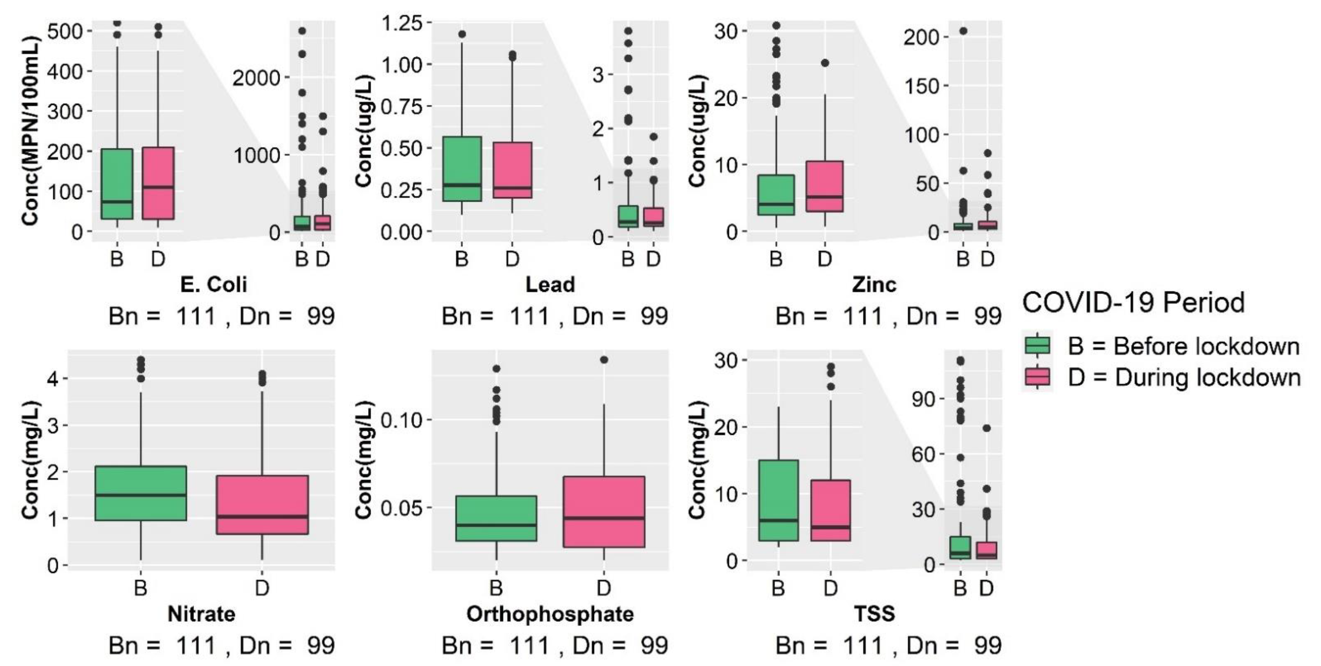
Similar to the seasonal analysis, the boxplots in Figure 3 demonstrate the distribution of all samples taken during the different periods from eligible stations. The smaller number of samples taken during the pandemic reflects fewer cases of extremely high concentrations as outliers in the boxplots. Table 2 reports the results of the Mann–Whitney test, as well as median pollutant values across COVID-19 periods. The test shows that nitrate is the only pollutant that received a statistically significant difference between the two periods (p < 0.05). The median nitrate concentration before COVID-19 was 1.5 mg/L, and it decreased to 1.04 mg/L in samples collected during the COVID-19 lockdown period.

3.3. Correlation between Water Quality and Explanatory Variables

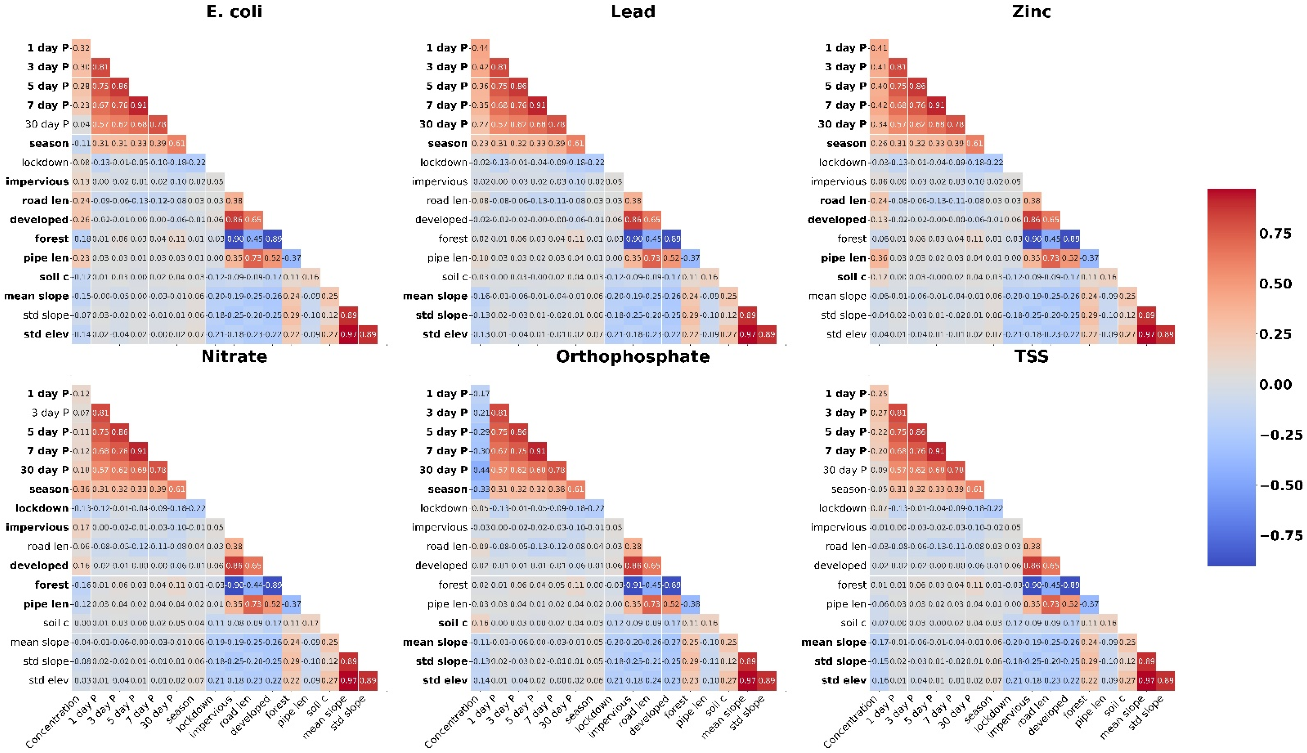
As shown in Figure 4, in nearly all cases, antecedent precipitation amounts are significantly correlated with all pollutants, although the strength of the relationship varies by pollutant. Nitrate’s correlation coefficients with all antecedent precipitation values are the lowest among all pollutants. Additionally, nitrate was the only pollutant that included the COVID-19 lockdown period as an input feature, reinforcing the findings in Table 2. Orthophosphate was the only pollutant that was negatively associated with the precipitation variables. Road length is positively associated with E. coli and zinc concentrations. Developed land and pipe length are positively related to the E. coli concentration, while forested land and soil C are negatively associated with the E. coli concentration. Topographic variables such as the mean slope, standard deviation of the slope, and standard deviation of elevation are statistically significantly related to the orthophosphate concentration.

3.4. Random Forest Regression Results

With the massive number of combinations that are possible as input features and desired output pairs, the Random Forest performs the best when the number of training data points is largest while the variance of the output is minimal [19]. In the models using correlated features as inputs, lead was the most difficult pollutant to make predictions for. It received an R2 value of 0.04 for the OLS model and an R2 value of 0.08 for the Random Forest, which were the poorest values for both models. The Random Forest achieved its best performance with orthophosphate, producing an RSME = 0.0, MAE = 0.01, MAPE of 25.3, and R2 values of 0.58. With the Random Forest model, TSS and nitrate follow orthophosphate with R2 values of 0.54 and 0.42, respectively.
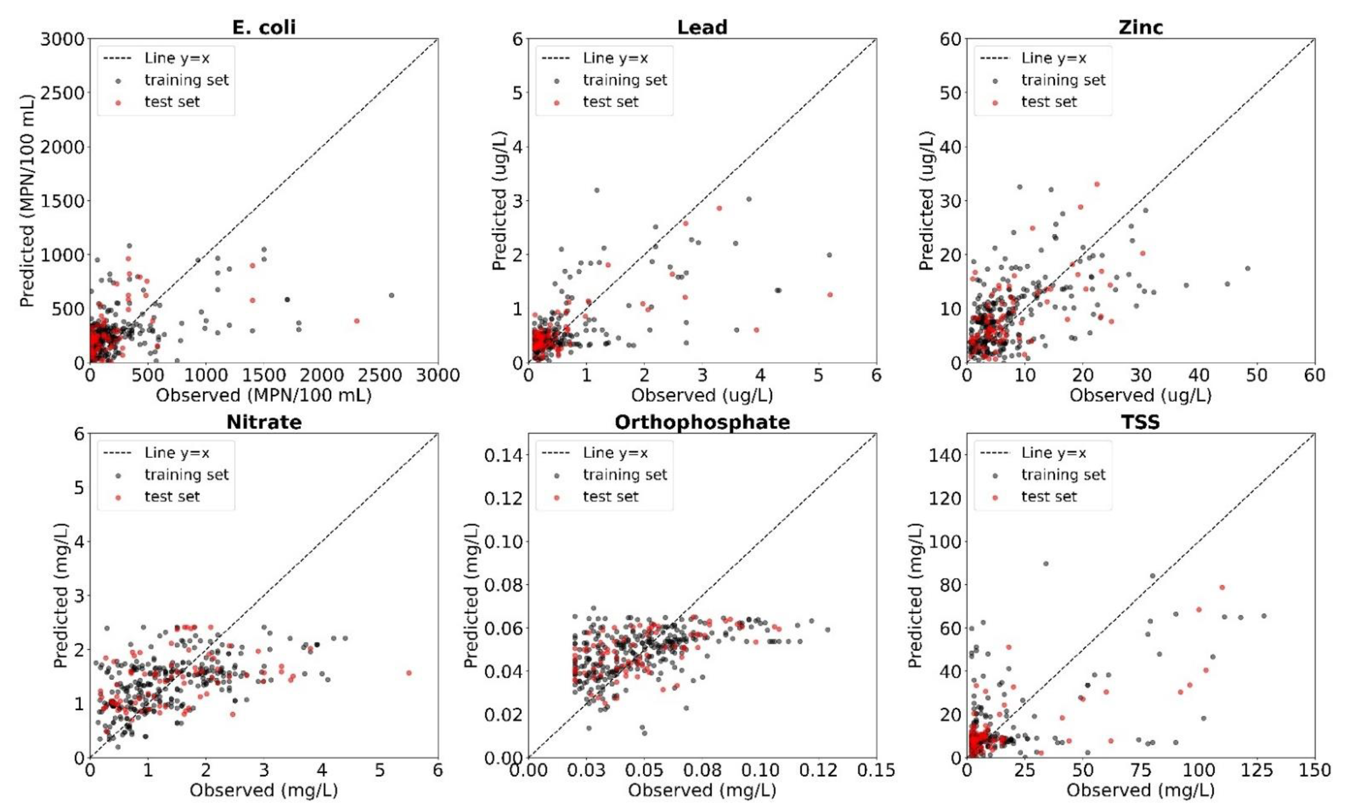
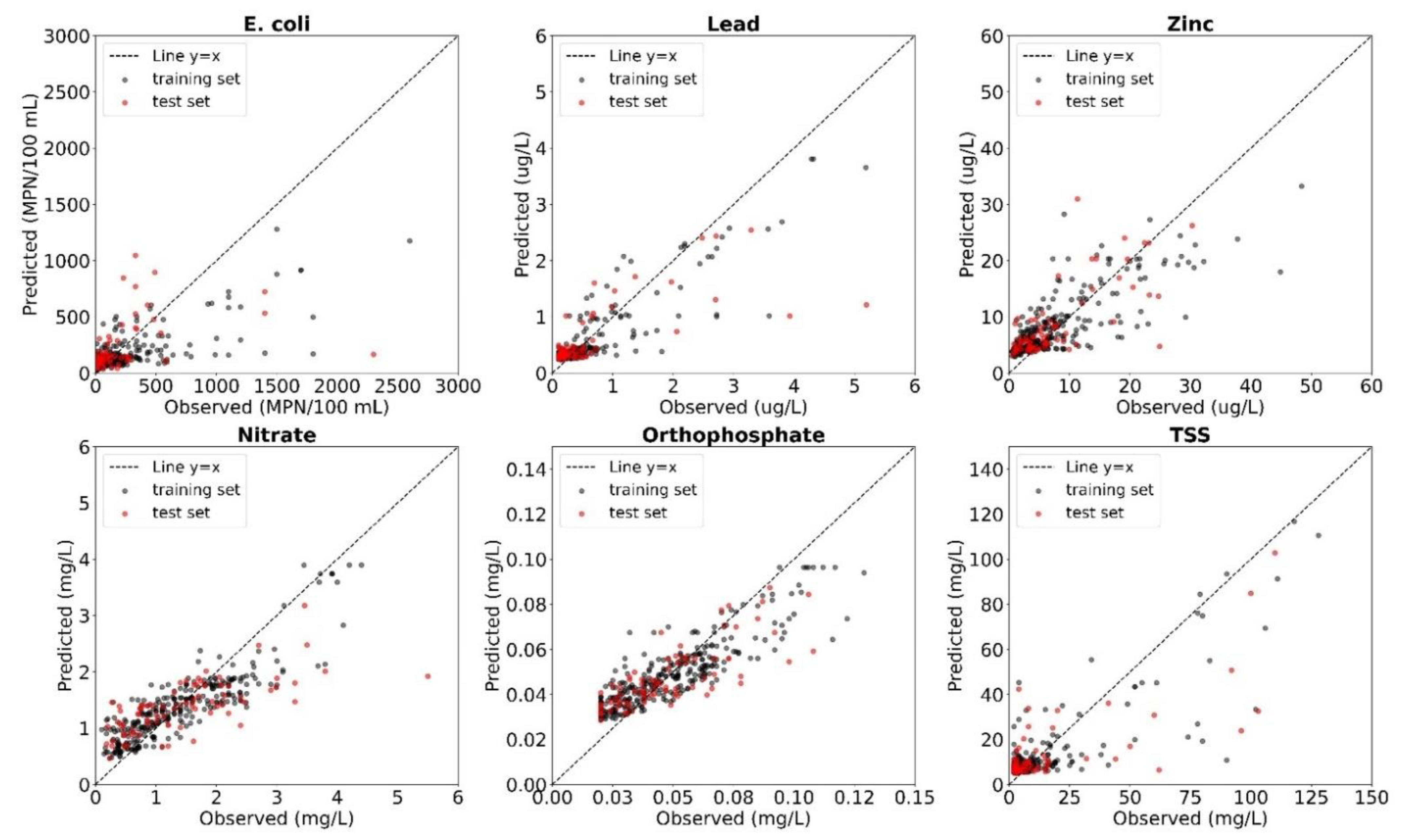
Comparing the R2 values for E. coli, the OLS model’s R2 value of 0.149 slightly outperformed the Random Forest’s R2 value of 0.13. For every other pollutant’s performance metrics, the Random Forest performed better than OLS, with lower RMSE, MAE, MAPE, values and a higher R2 value (Table 3). As shown in Figure 5 and Figure 6, the predictions made by the Random Forest are more clustered by the line of identity (Y = X). This fit is desired, as all the performance metrics calculate the total error from the predictions and their actual ground-truth values.

4. Discussion

E. coli and orthophosphate were the pollutants that had higher median values in the dry season. For E. coli, this confirms previous investigations of seasonal differences that found higher concentrations of the microorganism in urban watersheds in the summers in the Pacific Northwest [1]. With orthophosphate being negatively correlated with all five precipitation variables, it follows that the higher median value was achieved during the dry season. While the findings agree with a previous study in Johnson Creek in Portland [28], the results contradict other studies in humid temperate climates that reported higher concentrations of orthophosphate in the wet season [29,30]. Given that the main sources of orthophosphate in urban runoff are plant decay and plant fertilizers [7], climate plays a significant role in the orthophosphate concentration. During the wet winter season, fewer plants are decaying, and fertilizer usage diminishes because of the lower demand for lawn fertilizers. Together with fewer sources, more frequent winter precipitation could have resulted in the dilution of orthophosphate found in urban runoff, while groundwater might be a major source of orthophosphate in the dry season [28]. The heavy metals lead and zinc experienced higher median levels in the wet season with statistical significance. A flushing effect may be the cause of the increased heavy metal levels in the wet season in the study region. Similarly, a study in the Greater Vancouver region in Canada shows higher concentrations of lead and zinc in the wet season [31]. These findings are in contrast with the higher readings of both lead and zinc in the dry season in a semi-arid zone [7]. Differences between these investigations are likely to be attributed to differences in climate, the intensity of human activities, and the number of samples utilized for analysis.
The COVID-19 pandemic placed limitations on human activity, yet our analysis did not confirm many statistically significant changes in pollutant levels during the COVID-19 period, similar to the conclusion from a study on US coastal watershed health throughout the COVID-19 lockdown period [32]. Nitrate was the sole pollutant to have a statistically significant decrease in its measured concentration in urban storm runoff during the COVID-19 period. It is likely that the diminished car traffic might have resulted in lower emissions and atmospheric deposition of NOx, as reported in major Chinese cities [33,34]. The smaller number of samples taken during the lockdown period might have limited the detection of how urban streams responded to this sudden shift. Legislative responses and human attitudes toward following travel restrictions fluctuated temporally throughout different stages of the pandemic [35]. Changes in travel activity significantly varied spatially between areas defined as finely as the county level. This nonuniform response to the pandemic may have decreased the possibility for heavily trafficked areas to experience a clear improvement associated with the COVID-19 lockdown. Continually monitoring pollutant levels over a longer period as restrictions are lifted during the response to COVID-19 can provide a better understanding of how changes in human activities impact stormwater-runoff quality.
Spearman’s rank correlation analysis indicated one-day antecedent precipitation as an important explanatory variable for all pollutants, suggesting that the chosen pollutants are sensitive to short rainfall events. Other studies reported similar findings that turbidity and pathogen concentrations are highly correlated with the previous day’s precipitation in Tennessee, USA [36]. The positive correlation between zinc concentration and road length also confirms previous studies indicating that traffic on roads (e.g., car brake and tire wear) is the main source of zinc in urban streams [11,12,13]. The positive correlation between storm-pipe length and E. coli concentration indicates possible sources of human and animal wastes [37].
The Random Forest model outperformed standard OLS in modeling pollutant concentrations using a subset of the initial input features. Being allowed to include categorical data along with continuous precipitation and landscape data allows for a complete understanding of the factors that impact pollutant levels. While the RF model predicted naturally occurring pollutants (orthophosphate, TSS, and nitrate) reasonably well, it did not adequately predict anthropogenically generated pollutants (E. coli, lead, and zinc), suggesting that additional predictors are needed to improve the accuracy of the model. Further model-refining techniques such as boosting or interpreting the feature importance can allow a deeper understanding of how the Random Forest outperformed OLS, since both were trained using the same input features for each pollutant. Connecting a spatial aspect to a temporal analysis can offer a more complete understanding to devise a targeted plan to restore urban runoff and associated water quality to a more natural regime [38,39].
To improve the reliability and efficiency of the model, future research endeavors will consider conducting an uncertainty analysis to identify the best set of input variables and ensemble models [40]. Once continuous hydrometeorological data (e.g., precipitation and flow) are available, different lead times can be considered for inputs to machine learning models. For example, different wavelet-ANN models using the least-squares boosting ensemble and Bates–Granger techniques resulted in the more reliable and accurate forecasting of chlorophyll and salinity in Hilo Bay, Hawaii, USA [40].

5. Conclusions

Using a unique set of spatially intensive monitoring data in urban streams, the study’s main findings are summarized below.
(1) Pollutant concentrations in urban runoff demonstrated pronounced differences across seasons and marginal differences with respect to COVID-19 travel restrictions. E. coli and orthophosphate experienced higher median values in the dry season, with different sources being more common during that period. Nitrate was the only element that showed statistically significantly lower amounts after the introduction of COVID-19 restrictions, most likely resulting from reduced traffic emissions due to lower driving volumes during this period.
(2) Antecedent rainfall variables were correlated with the measurements of all the pollutants and were thus used as inputs to the Random Forest model. The one-day antecedent precipitation amount has the highest correlations with E. coli, lead, zinc, and TSS. Road length is positively associated with E. coli and zinc concentrations, suggesting that roads are the primary sources of these pollutants. The standard deviation of the slope is positively associated with both nitrate and orthophosphate concentrations.
(3) The Random Forest demonstrated a better capability to utilize both temporal (antecedent precipitation) factors and spatial (land cover) variables to predict pollutant concentrations compared to the standard OLS model. The Random Forest achieved lower RMSE, MAE, and MAPE values and higher R2 values for the predictions of every pollutant except E. coli. E. coli was the pollutant with the highest variance during the study periods, contributing to the difficulty of modeling it by both the Random Forest and OLS. Orthophosphate was best estimated with the given inputs.
Future studies can include improvements to the Random Forest model with boosting or cross-validation. Feature importance can be analyzed to correlate input features to learn whether the correlation is an optimal condition for feature selection.
Regardless, the current study demonstrates the utility of using both landscape and weather variables as inputs for the Random Forest model for predicting water quality in urban streams.

Author Contributions

Conceptualization, D.R. and H.C.; methodology, D.R. and H.C.; software, D.R. and K.G.; validation, D.R., H.C. and K.G.; formal analysis, D.R.; investigation, D.R. and H.C.; resources, D.R., K.G. and H.C.; data curation, D.R.; writing—original draft preparation, D.R.; writing—review and editing, D.R., H.C. and K.G.; visualization, D.R. and K.G.; supervision, H.C.; project administration, H.C.; funding acquisition, H.C. All authors have read and agreed to the published version of the manuscript.

Funding

This research was supported by the National Science Foundation under grant number 1758006.

Data Availability Statement

The data are available from the corresponding author.

Acknowledgments

The authors appreciate the National Science Foundation for supporting this research. Christof Teuscher and Adrian Jimenez provided informal feedback on the initial version of the manuscript. Chris Prescott at the City of Portland provided water quality data, without which this research would not have been possible. Thanks also go to three anonymous reviewers and editor, whose comments helped strengthen the manuscript.

Conflicts of Interest

The authors declare no conflict of interest. The funders had no role in the design of the study; in the collection, analyses, or interpretation of data; in the writing of the manuscript; or in the decision to publish the results.

References

  1. Chen, H.J.; Chang, H. Response of discharge, TSS, and E. coli to rainfall events in urban, suburban, and rural watersheds. Environ. Sci. Process. Impacts 2014, 16, 2313–2324. [Google Scholar] [CrossRef] [PubMed]
  2. Dwight, R.H.; Caplan, J.S.; Brinks, M.V.; Catlin, S.N.; Buescher, G.; Semenza, J.C. Influence of Variable Precipitation on Coastal Water Quality in Southern California. Water Environ. Res. 2011, 83, 2121–2130. [Google Scholar] [CrossRef] [PubMed]
  3. Fish, N.; Jordan, M. Portland Area Watershed Monitoring and Assessment Program. Executive Summary—Findings from Years 1–4. 2018. Available online: https://www.portlandoregon.gov/bes/article/689921 (accessed on 27 July 2021).
  4. Yazdi, M.N.; Sample, D.J.; Scott, D.; Wang, X.; Ketabchy, M. The effects of land use characteristics on urban stormwater quality and watershed pollutant loads. Sci. Total Environ. 2021, 773, 145358. [Google Scholar] [CrossRef] [PubMed]
  5. Guo, D.; Lintern, A.; Webb, J.A.; Ryu, D.; Liu, S.; Bende-Michl, U.; Leahy, P.; Wilson, P.; Western, A.W. Key Factors Affecting Temporal Variability in Stream Water Quality. Water Resour. Res. 2019, 55, 112–129. [Google Scholar] [CrossRef] [Green Version]
  6. Ferreira, C.S.S.; Walsh, R.P.D.; de Lourdes Costa, M.; Coelho, C.O.A.; Ferreira, A.J.D. Dynamics of surface water quality driven by distinct urbanization patterns and storms in a Portuguese peri-urban catchment. J. Soils Sediments 2016, 16, 2606–2621. [Google Scholar] [CrossRef] [Green Version]
  7. Ortiz-Hernández, J.; Lucho-Constantino, C.; Lizárraga-Mendiola, L.; Beltrán-Hernández, R.I.; Coronel-Olivares, C.; Vázquez-Rodríguez, G. Quality of urban runoff in wet and dry seasons: A case study in a semi-arid zone. Environ. Sci. Pollut. Res. 2016, 23, 25156–25168. [Google Scholar] [CrossRef] [PubMed]
  8. Mainali, J.; Chang, H.; Chun, Y. A review of spatial statistical approaches to modeling water quality. Prog. Phys. Geogr. Earth Environ. 2019, 43, 801–826. [Google Scholar] [CrossRef]
  9. Oregon Department of Transportation. TRAFFIC FLOW MAP 2020 [WWW Document]. Flow_Map_2020. 2020. Available online: https://www.oregon.gov/odot/Data/Documents/Flow_Map_2020.pdf (accessed on 30 July 2021).
  10. Oregon Department of Transportation. Impacts of COVID-19 on Traffic [WWW Document]. Region1 Covid-19 Traffic Report 20 08.03.20-09.23.20. 2021. Available online: https://www.oregon.gov/odot/Projects/Project%20Documents/Region1%20Covid-19%20Traffic%20Report%2020%2008.03.20-09.23.20.pdf (accessed on 30 July 2021).
  11. Beasley, G.; Kneale, P. Reviewing the impact of metals and PAHs on macroinvertebrates in urban watercourses. Prog. Phys. Geogr. Earth Environ. 2002, 26, 236–270. [Google Scholar] [CrossRef]
  12. Alexakis, D.E. Multielement Contamination of Land in the Margin of Highways. Land 2021, 10, 230. [Google Scholar] [CrossRef]
  13. Sansalone, J.J.; Buchberger, S.G. Partitioning and First Flush of Metals in Urban Roadway Storm Water. J. Environ. Eng. 1997, 123, 134–143. [Google Scholar] [CrossRef]
  14. Andoh, R.Y.G. Urban Runoff: Nature, Characteristics and Control. Water Environ. J. 1994, 8, 371–378. [Google Scholar] [CrossRef]
  15. Marsalek, J.; Rochfort, Q.; Brownlee, B.; Mayer, T.; Servos, M. An exploratory study of urban runoff toxicity. Water Sci. Technol. 1999, 39, 33–39. [Google Scholar] [CrossRef]
  16. Arefinia, A.; Bozorg-Haddad, O.; Chang, H. Chapter 4: The Role of Data Mining in Water Resources Management. In Essential Tools for Water Resources Analysis, Planning, and Management; Bozorg-Haddad, O., Ed.; Springer: Singapore, 2021. [Google Scholar]
  17. Nourani, V.; Molajou, A.; Tajbakhsh, A.D.; Najafi, H. A Wavelet Based Data Mining Technique for Suspended Sediment Load Modeling. Water Resour. Manag. 2019, 33, 1769–1784. [Google Scholar] [CrossRef]
  18. Wang, F.; Wang, Y.; Zhang, K.; Hu, M.; Weng, Q.; Zhang, H. Spatial heterogeneity modeling of water quality based on random forest regression and model interpretation. Environ. Res. 2021, 202, 111660. [Google Scholar] [CrossRef]
  19. Sakaa, B.; Elbeltagi, A.; Boudibi, S.; Chaffaï, H.; Islam, A.R.M.T.; Kulimushi, L.C.; Choudhari, P.; Hani, A.; Brouziyne, Y.; Wong, Y.J. Water quality index modeling using random forest and improved SMO algorithm for support vector machine in Saf-Saf river basin. Environ. Sci. Pollut. Res. 2022, 29, 48491–48508. [Google Scholar] [CrossRef]
  20. Chang, H. Comparative streamflow characteristics in urbanizing basins in the Portland Metropolitan Area, Oregon, USA. Hydrol. Process. 2007, 21, 211–222. [Google Scholar] [CrossRef]
  21. United States Geological Survey, 2021. City of Portland HYDRA Rainfall Network. Available online: https://or.water.usgs.gov/non-usgs/bes/ (accessed on 28 June 2021).
  22. City of Portland Environmental Services, n.d. Portland Area Watershed Monitoring and Assessment Program (PAWMAP). Available online: https://www.portlandoregon.gov/bes/article/489038 (accessed on 28 June 2021).
  23. Cooley, A.K.; Chang, H. Detecting change in precipitation indices using observed (1977–2016) and modeled future climate data in Portland, Oregon, USA. J. Water Clim. Change 2021, 12, 1135–1153. [Google Scholar] [CrossRef]
  24. McKinney, W. Data Structures for Statistical Computing in Python. In Proceedings of the 9th Python in Science Conference, Austin, TX, USA, 28 June–3 July 2010; Available online: https://conference.scipy.org/proceedings/scipy2010/pdfs/mckinney.pdf (accessed on 28 June 2021).
  25. Gelsey, K.; Chang, H.; Ramirez, D. Effects of Landscape Characteristics, Anthropogenic Factors, and Seasonality on Water Quality in Portland, Oregon; Portland State University: Portland, OR, USA, 2021. (In review) [Google Scholar]
  26. Breiman, L. Random Forest. Mach. Learn. 2001, 45, 5–32. [Google Scholar] [CrossRef] [Green Version]
  27. Pedregosa, F.; Varoquaux, G.; Gramfort, A.; Michel, V.; Thirion, B.; Grisel, O.; Blondel, M.; Prettenhofer, P.; Weiss, R.; Dubourg, V.; et al. Scikit-learn: Machine Learning in Python. J. Mach. Learn. Res. 2011, 12, 2825–2830. [Google Scholar]
  28. Sonoda, K.; Yeakley, J.A. Relative Effects of Land Use and Near-Stream Chemistry on Phosphorus in an Urban Stream. J. Environ. Qual. 2007, 36, 144–154. [Google Scholar] [CrossRef]
  29. Yang, Y.-Y.; Toor, G.S. Stormwater runoff driven phosphorus transport in an urban residential catchment: Implications for protecting water quality in urban watersheds. Sci. Rep. 2018, 8, 11681. [Google Scholar] [CrossRef] [PubMed]
  30. Hobbiea, S.E.; Finlaya, J.S.; Jankea, B.D.; Nidzgorskia, D.A.; Milletb, D.B.; Baker, L.A. Contrasting nitrogen and phosphorus budgets in urban watersheds and implications for managing urban water pollution. Proc. Natl. Acad. Sci. USA 2017, 114, 4177–4182. [Google Scholar] [CrossRef] [PubMed] [Green Version]
  31. Huang, J.Y.; Gergel, S.E. Landscape indicators as a tool for explaining heavy metal concentrations in urban streams. Landsc. Urban Plan. 2022, 220, 104331. [Google Scholar] [CrossRef]
  32. Wetz, M.S.; Powers, N.C.; Turner, J.W.; Huang, Y. No widespread signature of the COVID-19 quarantine period on water quality across a spectrum of coastal systems in the United States of America. Sci. Total Environ. 2022, 807, 150825. [Google Scholar] [CrossRef] [PubMed]
  33. Chen, H.; Huo, J.; Fu, Q.; Duan, Y.; Xiao, H.; Chen, J. Impact of quarantine measures on chemical compositions of PM2.5 during the COVID-19 epidemic in Shanghai, China. Sci. Total Environ. 2020, 743, 140758. [Google Scholar] [CrossRef]
  34. Yang, Y.; Zhao, T.; Jiao, H.; Wu, L.; Xiao, C.; Guo, X.; Jin, C. Atmospheric Organic Nitrogen Deposition in Strategic Water Sources of China after COVID-19 Lockdown. Int. J. Environ. Res. Public Health 2022, 19, 2734. [Google Scholar] [CrossRef]
  35. Bamney, A.; Gupta, N.; Jashami, H.; Megat-Johari, M.-U.; Savolainen, P. An Analysis of Changes in County-Level Travel Behavior Considering COVID-19–Related Travel Restrictions, Immunization Patterns, and Political Leanings. J. Transp. Eng. Part A Syst. 2022, 148, 04022096. [Google Scholar] [CrossRef]
  36. Hamilton, J.L.; Luffman, I. Precipitation, pathogens, and turbidity trends in the Little River, Tennessee. Phys. Geogr. 2009, 30, 236–248. [Google Scholar] [CrossRef]
  37. McCurdy, P.; Luffman, I.; Joyner, T.A.; Maier, K. Storm sampling to assess inclement weather impacts on water quality in a karst watershed: Sinking Creek, Watauga watershed, East Tennessee. J. Environ. Qual. 2021, 50, 429–440. [Google Scholar] [CrossRef]
  38. Chang, H.; Makido, Y.; Foster, E. Effects of land use change, wetland fragmentation, and best management practices on total suspended solids concentrations in an urbanizing Oregon watershed, USA. J. Environ. Manag. 2021, 282, 111962. [Google Scholar] [CrossRef]
  39. Fletcher, T.; Andrieu, H.; Hamel, P. Understanding, management and modelling of urban hydrology and its consequences for receiving waters: A state of the art. Adv. Water Resour. 2003, 51, 261–279. [Google Scholar] [CrossRef]
  40. Shamshirband, S.; Jafari Nodoushan, E.; Adolf, J.E.; Abdul Manaf, A.; Mosavi, A.; Chau, K.W. Ensemble models with uncertainty analysis for multi-day ahead forecasting of chlorophyll a concentration in coastal waters. Eng. Appl. Comput. Fluid Mech. 2019, 13, 91–101. [Google Scholar] [CrossRef]
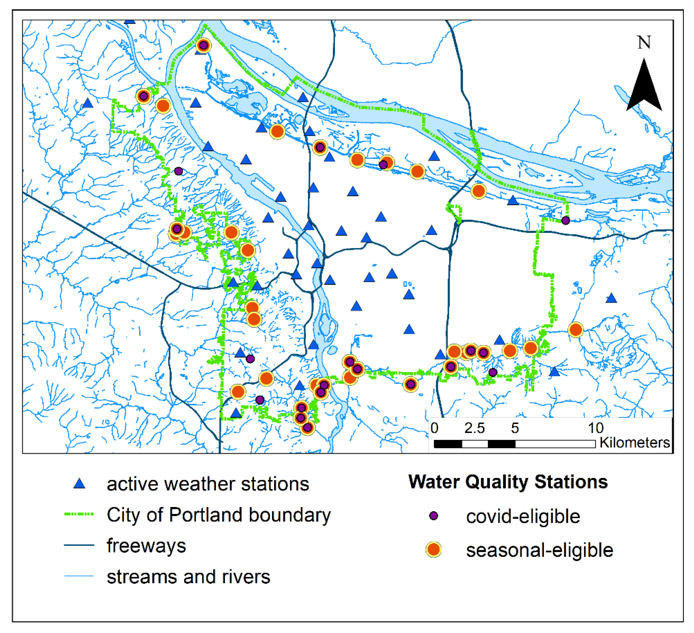
Figure 1. Study area: the city limits and locations of water quality monitoring and weather stations in Portland, OR, USA.
Hydrology 09 00220 g001
Figure 2. Boxplots showing the seasonal distributions of E. Coli, lead, zinc, nitrate, orthophosphate, and TSS concentration from 36 eligible stations.
Hydrology 09 00220 g002
Figure 3. Sample distribution across COVID-19 periods for E. Coli, lead, zinc, nitrate, orthophosphate, and TSS from 21 eligible stations.
Hydrology 09 00220 g003
Figure 4. Spearman’s rank correlation coefficient values among pollutant concentrations and explanatory variables. Statistically significant variables are shown in bold.
Hydrology 09 00220 g004
Figure 5. Comparison between observed and OLS-predicted pollutant concentrations.
Hydrology 09 00220 g005
Figure 6. Comparison between observed and Random-Forest-predicted pollutant concentrations.
Hydrology 09 00220 g006
Table 1. Median seasonal concentrations and Mann–Whitney U test p-values for samples originating from 36 eligible stations. Pollutants from anthropogenic sources are shaded yellow, while pollutants from more natural sources are shaded green. Bolded entries signify statistical significance (p < 0.05).
Pollutant (Units)Dry Season SamplesWet Season SamplesDry Season Median ConcentrationWet Season Median ConcentrationMann–Whitney
p-Value
E. coli (MPN/100 mL)14123612085.00.0029
Lead (μg/L)1412360.2240.315<0.001
Zinc (μg/L)1412363.785.705<0.001
TSS (mg/L)1412364.04.00.351
Nitrate (mg/L)1432360.721.5<0.001
Orthophosphate (mg/L)1422360.0540.038<0.001
Table 2. Mean concentrations and Mann–Whitney p-values for samples originating from 21 eligible stations during the COVID-19 period. Pollutants from anthropogenic sources are shaded yellow, while pollutants from more natural sources are shaded green. Bolded entries signify statistical significance (p < 0.05).
Pollutant (Units)Pre-COVID-19 SamplesCOVID-19 Lockdown SamplesPre-COVID-19 Median ConcentrationCOVID-19 Lockdown Median ConcentrationMann–Whitney Test p-Value
E. coli (MPN/100 mL)1119974.0110.00.75
Lead (μg/L)111990.2770.2610.61
Zinc (μg/L)111994.095.150.32
TSS (mg/L)111996.05.00.93
Nitrate (mg/L)111991.51.040.02
Orthophosphate (mg/L)111990.040.0440.71
Table 3. Comparison of model goodness-of-fit between Random Forest and OLS.
OLS
PollutantRSMEMAEMAPER2
E. coli321.09205.265.200.149
Lead2.110.570.970.042
Nitrate0.950.720.810.105
Orthophosphate0.000.0150.390.29
TSS18.2110.871.230.499
Zinc12.136.341.200.284
Random Forest
PollutantRSMEMAEMAPER2
E. coli323.68159.152.910.13
Lead2.070.530.770.08
Nitrate0.770.550.620.42
Orthophosphate0.000.010.250.58
TSS17.359.521.160.54
Zinc11.354.970.930.37
Publisher’s Note: MDPI stays neutral with regard to jurisdictional claims in published maps and institutional affiliations.