Hydrological and Hydraulic Flood Hazard Modeling in Poorly Gauged Catchments: An Analysis in Northern Italy

Abstract

Flood hazard is assessed for a watershed with scarce hydrological data in the lower plain of Northern Italy, where the current defense system is inadequate to protect a highly populated urban area located at a river confluence and crossed by numerous bridges. An integrated approach is adopted. Firstly, to overcome the scarcity of data, a regional flood frequency analysis is performed to derive synthetic design hydrographs, with an original approach to obtain the flow reduction curve from recorded water stages. The hydrographs are then imposed as upstream boundary conditions for hydraulic modeling using the fully 2D shallow water model PARFLOOD with the recently proposed inclusion of bridges. High-resolution simulations of the potential flooding in the urban center and surrounding areas are, therefore, performed as a novel extensive application of a truly 2D framework for bridge modeling. Moreover, simulated flooded areas and water levels, with and without bridges, are compared to quantify the interference of the crossing structures and to assess the effectiveness of a structural measure for flood hazard reduction, i.e., bridge adaptation. This work shows how the use of an integrated hydrological–hydraulic approach can be useful for infrastructure design and civil protection purposes in a poorly gauged watershed.

1. Introduction

Among the most frequent and destructive disasters, floods annually hit people in many countries all over the world. Flooding is the cause of up to 40% of natural disasters in the world, entailing almost half of the fatalities related to natural hazard, with a rising trend [1,2,3,4]. Flood risk management, therefore, has to be implemented on the basis of a proper and aware estimation of flood hazards under the consciousness that, due to global warming, the occurrence of extreme flood events will probably increase in the future, even if some recent studies show a situation that, at least in Europe, seems very patchy [5,6,7,8]. This task can be challenging, as it requires the careful consideration of many factors related to catchment properties, hydrological inputs, and characteristics of rural, urban, and productive areas that are potentially floodable [9]. Inaccurate hazard and risk assessments may result in poor risk management interventions, ranging from insufficient protection to squandering of public resources. Accurate flood hazard and risk assessments, on the contrary, can valuably support decisions on land use, design of infrastructure, and drafting and organization of emergency response for civil protection purposes. Inundation mapping allows capturing of the extent of the flooded area and can also represent a tool of primary importance to support first responders [10,11]. Whatever type of model is used for the purpose, a key element in flood risk assessment is the identification of the hydrological stresses to be adopted as input. Unfortunately, the definition of the hydrological inputs is strongly hindered by the fact that, very often, the watersheds of interest are devoid of reliable field observations. Adopting the definition of Sivapalan et al. [12], ungauged or poorly gauged basins are those in which quality and quantity of hydrological observations are inadequate to allow a reliable evaluation of streamflow. Always the object of ongoing investigation, the prediction or forecasting of the hydrological responses of these basins and the evaluation of the associated uncertainty were the subject of a significant research activity (Prediction in Ungauged Basins—PUB) by the scientific community through the decade 2003–2012 [12]. Rather disheartening results emerged from that analysis, according to which the majority of rivers and stream reaches, and tributaries in the world are ungauged or poorly gauged [13]. Indeed, the knowledge of continuous water stages and discharges in rivers is a crucial factor in watershed analyses and water resource management, due to the need to evaluate flood peaks, flow reduction factors, and duration curves at the basis of the design of engineering structures, such as defense systems, flood detention reservoirs, etc. Very often, unfortunately, even for watersheds with a good consistency of water stage observations, both as regards the length of the measured series and the density of the gauging stations along the river network, the poor reliability or even the unavailability of the stage–discharge relationships affects the potential of the observed database. This could be obviated by developing methodologies capable of extracting useful information for the construction of flow hydrographs directly from water-stage-observed time series.

A possible solution to overcome the lack of direct observations is to resort to regionalization techniques that allow the necessary information to be derived from the knowledge of quantitative data in nearby gauged watersheds or with reference to a region homogeneous with the ungauged or poorly gauged catchment under investigation [14]. Behind the concept of a homogeneous region, there is the assumption that the similitude in climatic, geologic, vegetative, topographic, etc., characteristics would give origin to similar responses in terms of runoff. This does not necessarily imply the neighborhood of the basins [15]. Regionalization can be intended as the process of transferring hydrological information from gauged to poorly gauged watersheds, also, in terms of frequency [16,17,18]. It is obviously advisable to use any direct information available for the area of interest, even if scarce and fragmentary, to validate, to some extent, its belonging to the identified homogeneous region [19,20]. Many sources of uncertainty can affect the prediction reliability due to data and to the regionalization procedure itself, and this issue is constantly subject to attention given the importance that regionalization procedures play in hydrology [21,22,23,24].

In general, once the hydrological inputs of assigned probable frequency have been identified, inundation mapping can be performed through distinct approaches [25]: simplified conceptual procedures, empirical methods, and physically based models. The latter are often run at low resolution to allow reasonable computational times with the aim of creating flooding maps, sometimes also at a continental scale [26,27,28,29]. Even if a line of research [30,31,32] argued that inundation mapping performed at high spatial resolution can lead to useless and even counterproductive detail, there is evidence that high-resolution meshes derived from LiDAR-based DTMs allow a detailed description of the relevant terrain features typical of man-made landscapes (e.g., roads, railways, channels, and embankments) that dominate flow patterns and that would be undetectable at a coarse resolution [33,34,35,36]. The use of GPU-accelerated 2D shallow water numerical models and the adoption of nonuniform grids represent a powerful analysis tool, allowing a drastic reduction in the computational costs [11,37]. Care has to be devoted, anyway, to an in-depth analysis of the terrain model, which, even in the presence of high spatial resolution, could be affected by non-negligible descriptive deficiencies, such as those occurring during vegetation filtering along streams with densely vegetated banks [38]. Anyway, the most accurate results for flood modeling are obtained adopting a fine spatial resolution, also, thanks to the accurate description of local terrain features and hydraulic structures that can be achieved [34,39].

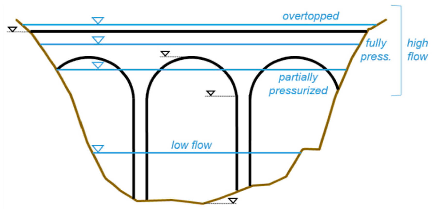
Flood propagation in rivers and channels is significantly affected by the presence of bridges and other crossing structures, which represent an obstruction to the flow due to lateral and vertical constrictions and increase the hazard in upstream areas as a consequence of the backwater effect. Moreover, in the presence of high return period flood events, bridge decks may even experience overtopping; it is, therefore, appropriate that all the elements interfering with the flow would be properly considered in numerical simulations aimed at flood management purposes [40]. Different approaches can be adopted to include the presence of bridges in 2D shallow water models [41,42], and the choice of the modeling approach should also consider the possible additional computational burden consequent to the introduction of the necessary solution algorithms. A possible way to simulate the presence of bridges and other hydraulic structures in 2D domains is the implementation of internal boundary conditions [43]. Recent studies investigated the possibility to also implement this approach in GPU-accelerated numerical codes [44], and the validations performed provided good results, both in low- and high-flow conditions for bridges, without affecting the performance of the calculation tools. It is, in fact, very important to preserve the computational efficiency of the numerical codes, both with a view to effectively simulate flooding phenomena on very extensive computing domains and to achieve efficient and accurate 2D simulations in ever shorter calculation times.

With the aim of assessing flood hazard in a poorly gauged watershed in Northern Italy, an integrated hydrologic–hydraulic approach is adopted here. A regional flood frequency analysis is performed to derive synthetic design hydrographs (SDH) to be imposed as upstream boundary conditions for fully 2D high-resolution hydraulic modeling in a domain in which an urban center is located at the confluence of two streams. An original approach is studied to obtain indispensable information for the construction of SDHs by exploiting the knowledge of the behavior of water stage hydrographs instead of discharge ones. Water stage hydrographs are, indeed, usually more accessible and reliable than discharge hydrographs due to the unavailability or uncertainty of the stage–discharge relationships.

The area of interest is characterized by the presence of over 20 crossing structures. This then leads to an extensive application of bridge modeling in a truly 2D framework for each different scenario. Thanks to the high efficiency of the code architecture and bridge computational approach, this entails only a negligible increase in the calculation times compared to the simulation of the same scenario in the absence of the crossing structures. Therefore, the computed flooded areas and water levels, in the actual state and in the hypothetical absence of bridges, are compared for each return period to quantify the influence exerted by the interfering structures upon flooding extent and to assess the effectiveness of a structural measure for flood hazard reduction, i.e., bridge rebuilding.

The paper is organized as follows. The study area is introduced in Section 2, while the hydrological analysis is presented in Section 3. In Section 4, the characteristics and set-up of the model and of the different flooding scenarios considered are illustrated. The results thus obtained are presented in detail in Section 5. The discussion and conclusions are then drawn in Section 6.

2. Study Area

The Chiavenna is a left tributary of the Po River (the main Italian watercourse). It is about 52 km long and flows in the northwest of the Emilia-Romagna region (Northern Italy); its narrow and elongated catchment, which also collects the waters of the Riglio and Chero streams, has a total area of 340 km² (Figure 1 and

Table 1. Watershed characteristics and mean annual rainfall for contributing areas at the gauging stations of interest for the period 1997–2018.

Watercourse	Gauging Station	Area, A (km2)	Main Branch Length, Lmb (km)	Average Altitude 1, Hmed (m)	Mean Annual Rainfall (mm)
Chero	Ciriano	56	25	323	962
Chiavenna	Saliceto	161	37	235	876
Riglio	Montanaro	116	30	227	846

¹ Above the gauging station.

), about 40% of which is hilly and mountainous. The character of the river system is typically torrential, and not infrequently, in summer, the riverbeds are totally dry.

3. Hydrological Analysis

With the aim of assessing the hydrological inputs for the hydraulic simulations, design hydrographs of an assigned return period have to be evaluated. They can be completely determined once the peak discharge frequency distribution and the shapes of the hydrographs are identified at the sites of interest. Of course, these features should be inferred from the analysis of historical flood hydrographs at the chosen boundary condition sections, if available. However, the fragmentary or not totally reliable knowledge of the historical flood waves makes it necessary to partly resort to regional techniques.

3.1. Available Data

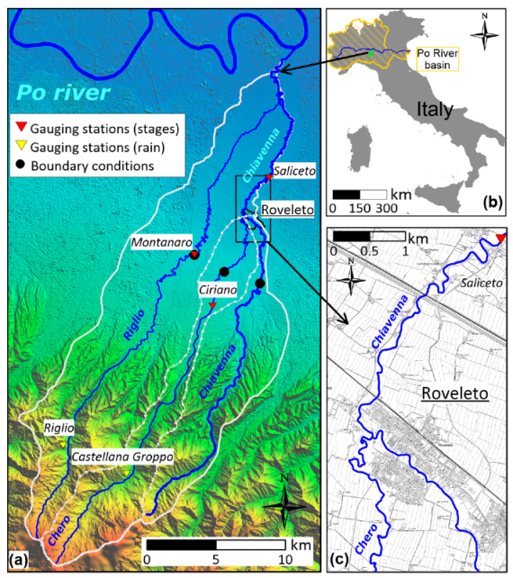
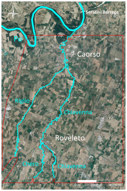
The historical rainfall data available for the Chiavenna basin refer to the gauging stations of Castellana Groppo (1983–2001) and Riglio (2003–2018). The available records at the two sites were joined into a unique sample of 35 years due to the proximity and similar properties. The gauging sites are, in fact, only about 5 km away (Figure 1) and at the same altitude above sea level (434 m and 432 m for Castellana Groppo and Riglio, respectively), without any noteworthy difference in topographic parameters, such as slope gradient and exposition, capable of significantly influencing the local rainfall patterns. The main characteristics of the rainfall data samples confirm the possibility of merging them in a unique sample (

Table 2. Characteristics of the rainfall data samples.

Data Sample	Period	Size	1-h Rainfall		Daily Rainfall
			Mean (mm)	St. Dev. (mm)	Mean (mm)	St. Dev. (mm)
Castellana Groppo	1983–2001	19	24.3	11.2	66.9	14.5
Riglio	2003–2018	16	23.9	9.5	64.6	17.0
Unique	1983–2018	35	24.1	10.3	65.9	15.5

).

With reference to the analysis of the historical rainfall unique sample, it is worthwhile stressing two significant values, namely the average values of the 1-h m(h₁) and daily m(h_d) maximum annual rainfall, equal to 24.1 mm and 65.9 mm, respectively (Table 2). These values may be of some interest if regionalization techniques at the outlet of contributing areas along the watercourses have to be adopted in the absence of reliable direct flow records.

Three hydrometric stations are present on the three main streams (Figure 1). For these outlets, watershed main characteristics, together with the mean annual rainfall are reported in Table 1.

For the gauging station on the Chero at Ciriano, frequent lacks and anomalies throughout the available water stage records (since 2002) and the absence of a reliable stage–discharge relationship made the data hardly usable.

The water stage records on the Riglio at Montanaro, instead, provide sufficient accuracy and completeness to determine average values. In particular, a series of 18 historical flood events can be identified. Unfortunately, for this station, the official stage–discharge relationships show excessive variability over the years, probably due to the difficulty in acquiring direct discharge measures. It was, therefore, decided not to rely on the flow records derived through the stage–discharge conversions, but, rather, only on the water stages.

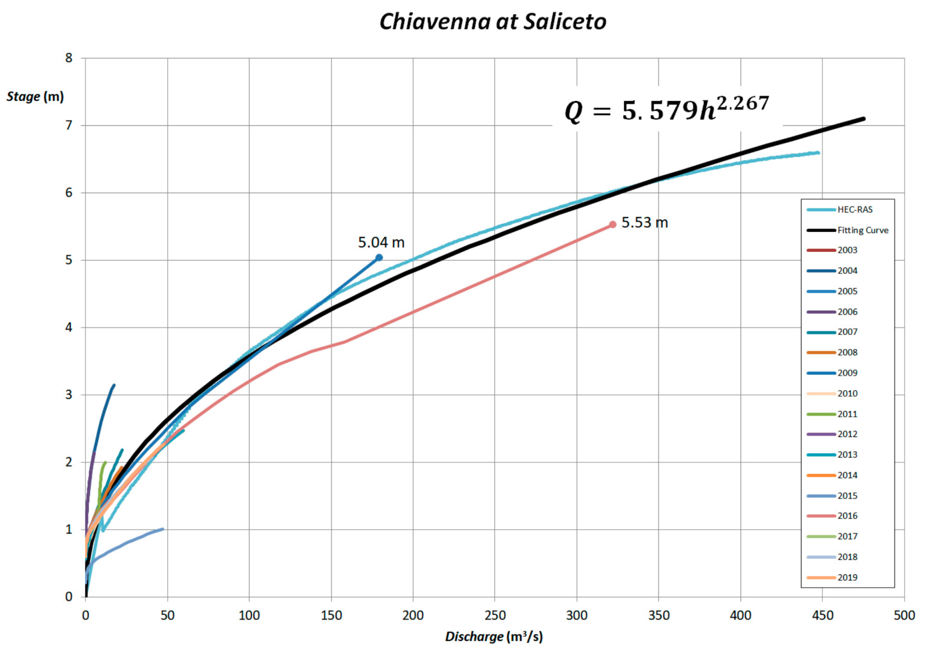
Moreover, the water stages recorded on the Chiavenna at Saliceto appear to be of fairly good quality, and this encourages their analysis with the aim of determining SDHs. As for the previous gauging station, however, the stage–discharge relationships show discordant and sometimes anomalous trends over the years (Figure 2). For this reason, a rating curve was derived through 1D hydraulic modeling, thanks to the availability of river cross-sectional surveys made specifically for this study. Values for Strickler’s roughness coefficient equal to 30 and 15 m^1/3 s⁻¹ were assumed for the main channel and the floodplains, respectively, and a monomial function of the form Q = aℎ^𝑏 was fitted to the numerical stage–discharge relation computed at the gauging site (a = 5.579 m^3−b s⁻¹, and b = 2.267). From Figure 2, it can be observed that this numerical rating curve is in fairly good agreement with the 2009 official stage–discharge relationship. From the conversion of the recorded hydrographs using the interpolated stage–discharge relationship, the average value of the annual maximum series (AMS) of N flood peaks (N = 18 events) was evaluated, resulting in 94.8 m³ s⁻¹. It is good to keep this value in mind for considerations that will be made in the following.

Due to the size of the available sample, the observed flood hydrographs can, of course, be trusted for the evaluation of reliable average values and for the identification of a shape of the hydrographs typical of the site of interest. On the other hand, such a reduced sample size is not enough to allow a reliable estimate of maximum values for the high return periods to be investigated in flood hazard assessment. It is, therefore, advisable to resort to alternative methodologies. As a consequence, the peak flow quantiles were estimated through a regional analysis, which requires the evaluation of an index flood and of a growth factor, a dimensionless function increasing with the return period, that allows the identification of the peak flow values for the return periods of interest once multiplied by the index flood.

3.2. Peak Discharge Estimation

3.2.1. Index Flood

Regionalization procedures allow exploitation of the observations available for a group of watersheds sharing similar behavior and gathered in a homogeneous region to which the catchment of interest is believed to belong, due to geographic location or characteristics. In general, a regionalization procedure is accomplished, first of all, through the determination of a flow scale factor proper of the site of interest, independent of the return period, namely the index flood [45,46]. Index flood is often assumed to be equal to the average of the annual maximum peak flows at the site of interest. Alternatively, it is possible to resort to indirect methods. Among others, multi-regressive models that express the index flood as a function of some significant features of the basin and of the watercourse can be adopted [45,46,47,48].

With reference to [45,46,47,48], two multi-regressive expressions for the index flood at the river sections of interest were evaluated. In the first, the area A of the catchment, the length L_mb of the main branch, and the hourly rain value m(h₁) are taken into consideration:

$$Q_{I1}=2.797·{10}^{-5}{A}^{1.235}m{\left(h_1\right)}^{3.513}{L}_{mb}^{-0.72},$$

(1)

while, in the second, the index flood is calculated with reference to the area A of the catchment, the average altitude H_med of the basin at the section of interest, and the pluvial average value relating to the daily rainfall m(h_d):

$$Q_{I2}=2.1·{10}^{-4}{A}^{1.082}m{\left(h_d\right)}^{2.416}{H}_{med}^{-0.469}$$

(2)

For the Chiavenna basin (from [45,49]), it is possible to estimate the values of 26 mm and 66 mm, respectively, for m(h₁) and m(h_d). These values are in very good agreement with the corresponding values of 24.1 mm and 65.9 mm obtained from the rain sample introduced in Section 3.1.

The application of Equations (1) and (2) leads to the values shown in

Table 3. Index floods for the gauging stations of interest (selected values in bold type).

Watercourse	Gauging Station	Index Flood Equation (1) QI1 (m3 s−1)	Index Flood Equation (2) QI2 (m3 s−1)
Chero	Ciriano	37	27
Chiavenna	Saliceto	103	98
Riglio	Montanaro	80	70

. For the Chiavenna at Saliceto, it is observed that the index flood obtained with the two different multi-regressive relationships is in good agreement with the value obtained analyzing the at site flood waves, equal to 94.8 m³ s⁻¹, evaluated in Section 3.1. As a precautionary choice, the maximum values provided by the regressive relations at the sections of interest, which correspond to the outcome of Equation (1), will be adopted (bolded in Table 3).

3.2.2. Growth Factor

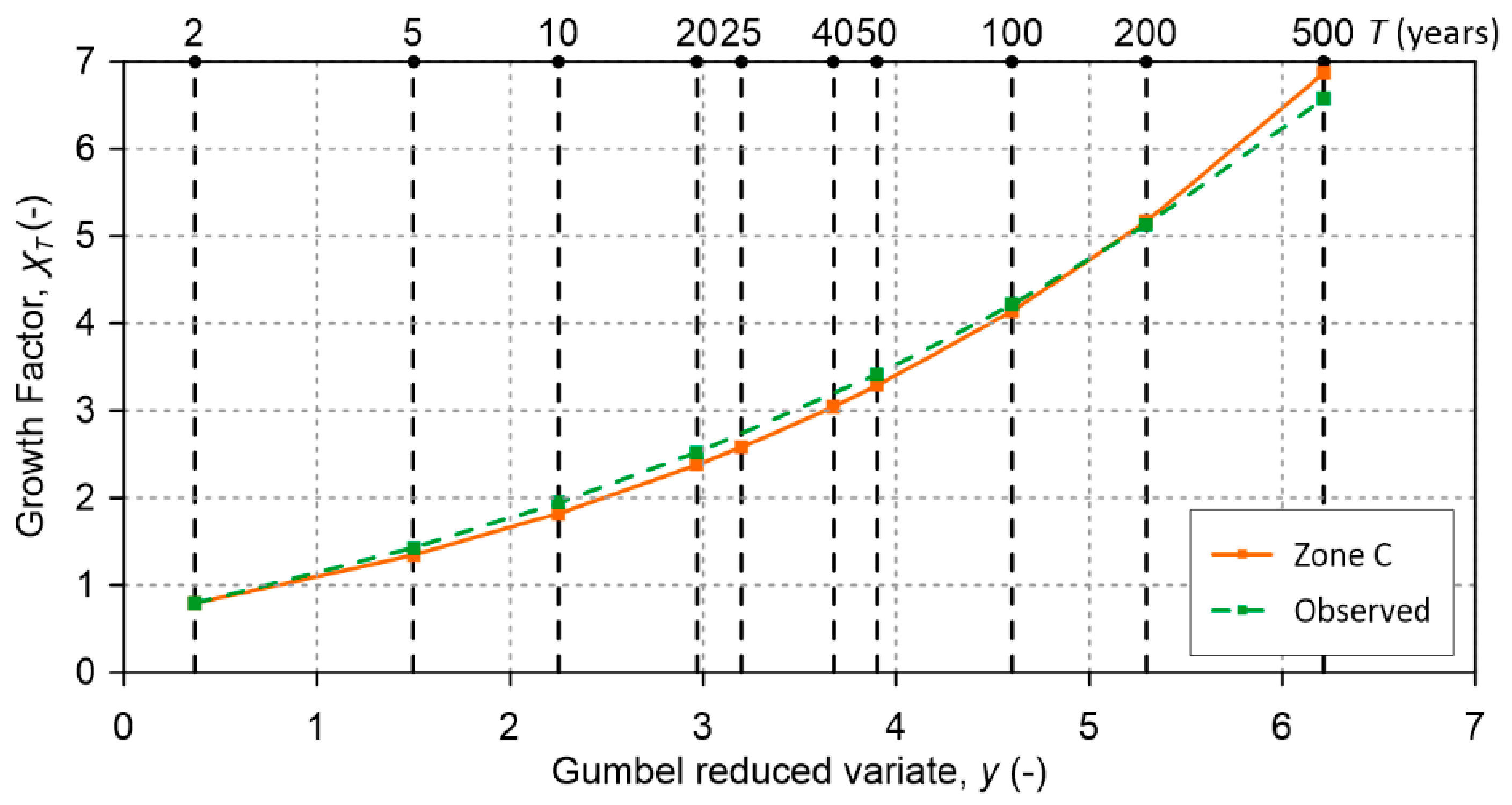
The VA.PI. project [48] and the following in-depth studies divided the Italian territory into different macro-regions that were, in turn, subdivided into homogeneous zones, each characterized by a different growth factor. For the different areas of the macro-regions, the growth curves were obtained from the analysis of the multiple gauging stations present in the considered territory and provided with reliable stage–discharge relationships. The growth factor is identified on the basis of a GEV distribution having expression:

$${\chi }_T=\xi +\frac{\alpha }{\kappa }\left[1-e^{-\kappa y}\right]$$

(3)

in which y is the Gumbel reduced variate. With regard to Zone C, the closer to the Chiavenna basin, the three parameters $\xi , \alpha \mathrm{and} \kappa$ in Equation (3) assume the values 0.643, 0.377, and −0.276, respectively.

Other studies have been based on an updated version of the original database of the VA.PI. project and have further divided the Emilia-Romagna–Marche region into sub-regions, each with its own growth curve [45,46,47,50].

The growth curve relating to the Zone C region can be compared with that deduced from the analysis of the series of maximum annual peak flows in Saliceto. The sample is well interpreted by a GEV distribution from which a growth factor close to that of Zone C is derived, as shown in Figure 3.

From the index floods and growth factors derived from the previous analyses, the peak discharges were obtained at the sites of interest simply by multiplying the maximum index flood by the growth factor for the chosen return periods of 20, 50, 200, and 500 years (

Table 4. Peak discharges for the chosen return periods at the sites of interest.

Watercourse	Gauging Station	Max. Index Flood QI Max (m3 s−1)	Peak Discharges
			Q20 (m3 s−1)	Q50 (m3 s−1)	Q200 (m3 s−1)	Q500 (m3 s−1)
Chero	Ciriano	37	88	122	191	254
Chiavenna	Saliceto	103	245	339	532	707
Riglio	Montanaro	80	190	263	413	549

).

3.3. Definition of the Design Hydrographs

3.3.1. Flow Reduction Curve and Peak Position Ratio

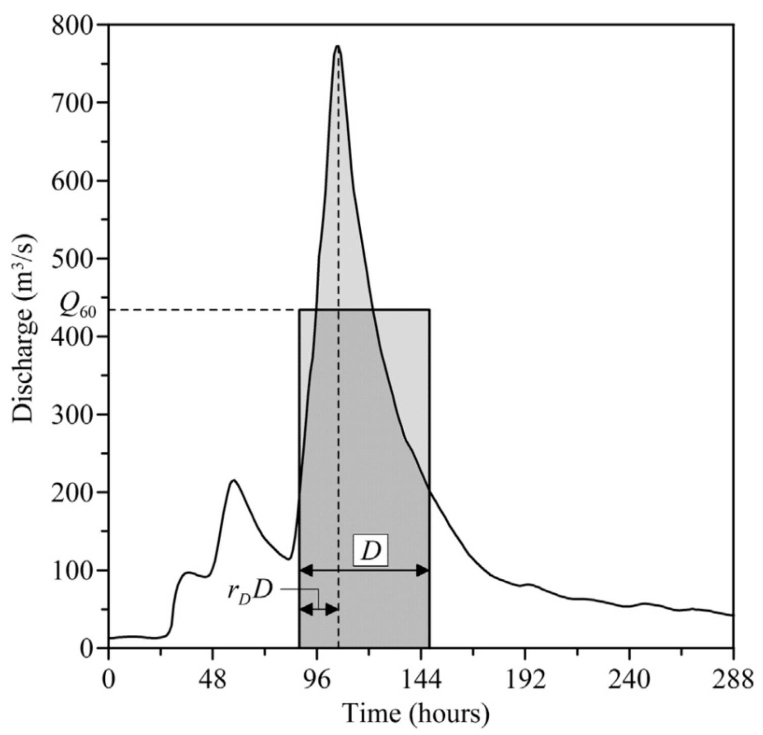
In order to evaluate hazard and risk maps, it is also necessary to estimate the characteristic volumes of the floods and their shape at the site of interest. These features are well represented by the reduction factor ε_D(T):

$${\epsilon }_D\left(T\right)=\frac{{\overline{Q}}_D\left(T\right)}{Q_0\left(T\right)}$$

(4)

where $Q_0\left(T\right)$ is the peak discharge of T years return period and ${\overline{Q}}_D\left(T\right)$ is the average discharge over the duration D of the same return period, and by the position r_D (0 ≤ r_D ≤ 1) of the peak of the hydrographs in the same intervals (Figure 4). Some methodologies for identifying the reduction factor and peak position are available for instrumented river sections, where a series of historical floods has been recorded, and for which a reliable stage–discharge relationship is available. In the absence of the second condition, the reduction curve can be inferred, after appropriate processing, on the basis of the trend of the water stages instead of discharges. If water stages are also not available, as for the majority of non-instrumented river sections, some indirect methods still allow the estimation of the reduction factor and peak position through empirical regional relations, which express them as a function of some characteristics of the basin under consideration [51].

In the present case, the water stage series recorded at Saliceto was analyzed directly and after its conversion into discharges through the rating curve previously derived. By analyzing the N available flow hydrographs with N_D moving windows, it was then possible to extract N_D samples with the size N for the value of the maximum annual average flow and (N_D − 1) samples for the peak position ratio for the durations of interest (for the duration 0 the position of the peak is, in fact, not defined). The choice of the maximum window duration D_f must derive from a preliminary examination of the characteristic durations of the most significant historical flood hydrographs. For the Chiavenna stream at the gauging site of Saliceto, durations from 0 to 96 h on an hourly basis were considered (D_f = 96 h, N_D = 97).

Although, in the general case, the reduction ratio ε_D is a function of duration D and return period T, in many practical cases, it can be assumed independent of the latter. This is strictly true only if—neglecting the influence of the statistical moments higher than the second—the coefficient of variation $CV\left({\overline{Q}}_D\right)$ and the probability distribution type of ${\overline{Q}}_D$ can be considered independent of D. Under these assumptions, ε_D becomes independent of T and reduces to the ratio of the averages of ${\overline{Q}}_D$ and $Q_0$:

$${\epsilon }_D=\frac{\mu \left({\overline{Q}}_D\right)}{\mu \left(Q_0\right)}$$

(5)

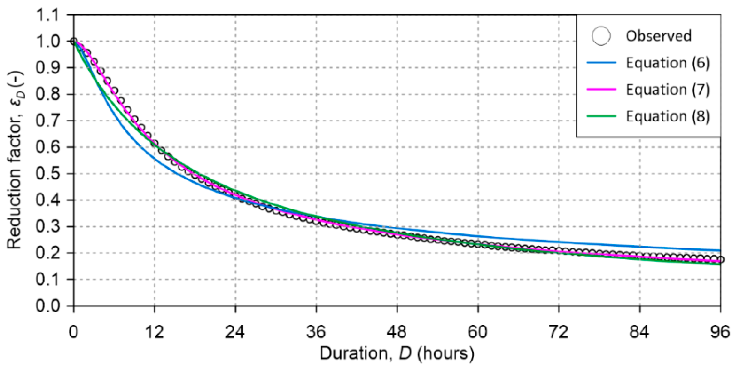
The expression of the reduction curve through a continuous and differentiable function of D, depending on the fewest possible parameters, can be advantageous. Based on the crossing properties of a given threshold value from continuous Gaussian stationary stochastic processes, [52] derived the following theoretical formulation:

$${\epsilon }_D=\sqrt{\frac{\theta }{2D}\left[2+e^{-\frac{4D}{\theta }}-\frac{3\theta }{4D}\left(1-e^{-\frac{4D}{\theta }}\right)\right]}$$

(6)

Besides the advantages coming from a theoretical basis and from the presence of a unique time parameter $\theta$, Equation (6) is particularly suitable to fit the empirical reduction ratios of large catchments. Moreover, [53] showed that $\theta$ can be strictly correlated to the time of concentration of the catchment.

For medium-size catchments (area between 100 and 1000 km²) [54], like the one considered here, Equation (6) does not accurately fit the empirical reduction factor (Figure 5). It was, therefore, decided to adopt the following generalized form:

$${\epsilon }_D={\left[\frac{\theta }{2D}\left[2+e^{-\frac{4D}{\theta }}-\frac{3\theta }{4D}\left(1-e^{-\frac{4D}{\theta }}\right)\right]\right]}^{\beta }$$

(7)

The higher flexibility given by the two parameters (θ and β) allows a better fit for the sample values (here β = 0.7 and θ = 7.95 h) (Figure 5). It is worth noting that other commonly adopted two-parameter functions, such as the one suggested by [16]:

$${\epsilon }_D={\left(1+\gamma D\right)}^{-\delta }$$

(8)

where $\gamma$ and $\delta$ are positive parameters, do not fit the empirical data in this case as well (Figure 5).

An interesting result can be obtained applying the same procedure to the water stage time series instead of to the discharge time series. If the stage–discharge relationship can be expressed by means of a monomial function of the type adopted in Section 3.1, a very good agreement between the reduction curve determined from the discharges and the one determined on the basis of the flood stages is achieved if the following transformation is adopted:

$${\epsilon }_{D\left|Q\right.}\cong {\epsilon }_{D\left|h\right.}{}^{\lambda b}$$

(9)

where b is the exponent of the stage–discharge relationship expressed in monomial form and λ is a corrective coefficient close to 1. For the Chiavenna at Saliceto, Equation (9) is satisfied in a very good way when λ is equal to the value 0.91 (Figure 6).

This result, even if it must be confirmed with further studies, allowed expansion of the analysis, also, to the station on the Riglio stream, for which a reliable stage–discharge relationship was not available.

In the almost total lack of useful observations for the Chero stream, and given the similarity among the watercourses under investigation, it was decided to adopt the same flow reduction factor and peak position ratio relations (i.e., the same waveform) obtained for the Saliceto gauging station for the Chero stream also.

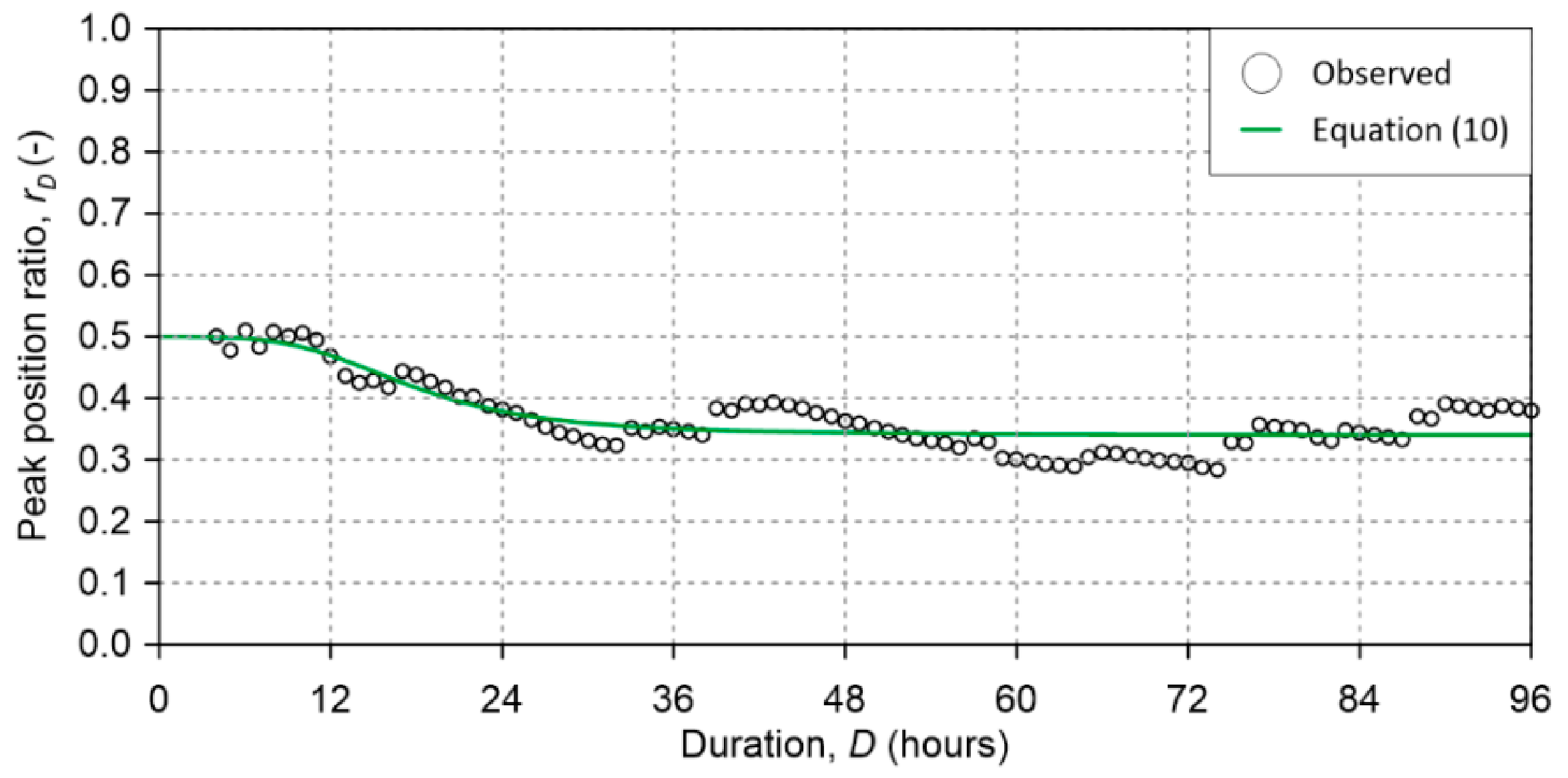
With regard to the expression of the peak position ratio introduced above, a continuous and differentiable function of D can be useful. N_D time series of observed peak position ratios are available for the Saliceto gauging station, one for each duration considered. For the purpose of the evaluation of the SDH, the average value of each series was calculated and the N_D values thus achieved were interpolated with the expression:

$$r_D\left(D\right)=a_1+\frac{a_2}{a_3+{\left(D\right)}^{a_4}}$$

(10)

imposing r_D(0) = 0.5 (Figure 7).

3.3.2. Evaluation of the SDHs

Following [55], the evaluation of the synthetic design hydrographs (SDHs) is carried out by imposing that the maximum average discharge in each duration coincides with the one predicted by the reduction curve. The shape of the hydrographs is then determined by the peak position ratio behavior.

The synthetic hydrograph is, therefore, defined by the conditions:

$$\underset{-r_{D}D}{\overset{0}{{\displaystyle \int }}}Q\left(\tau ;T\right)d\tau =r_D{\overline{Q}}_D\left(T\right)D; \underset{0}{\overset{\left(1-r_D\right)D}{{\displaystyle \int }}}Q\left(\tau ;T\right)d\tau =r_D\left(1-r_D\right){\overline{Q}}_D\left(T\right)D$$

(11)

The evaluation of the two branches of the hydrograph Q(t; T), before and after the peak, is obtained by differentiating Equation (11) with respect to duration D [55] once the expression for the quantiles of the average maximum flow rate as a function of the reduction factor is introduced:

$${\overline{Q}}_D\left(T\right)={\epsilon }_D{Q}_0\left(T\right)$$

(12)

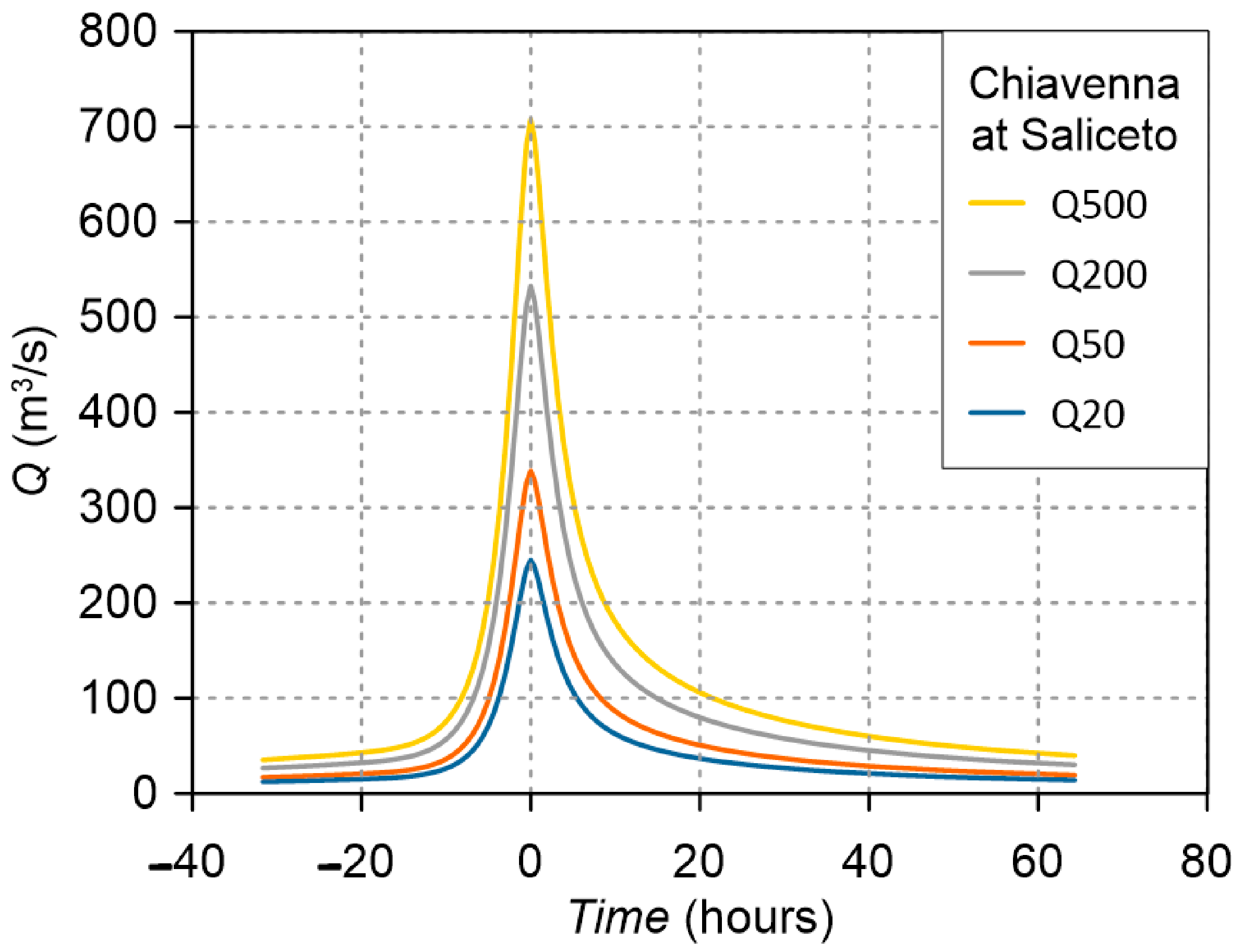
Once the index flood, the growth factor, the reduction factor, and the peak position are evaluated, it is possible to identify the set of SDHs for each section of interest and for the chosen return periods. As an example, Figure 8 shows the SDHs obtained through the adoption of the described procedure for the gauging station of Saliceto.

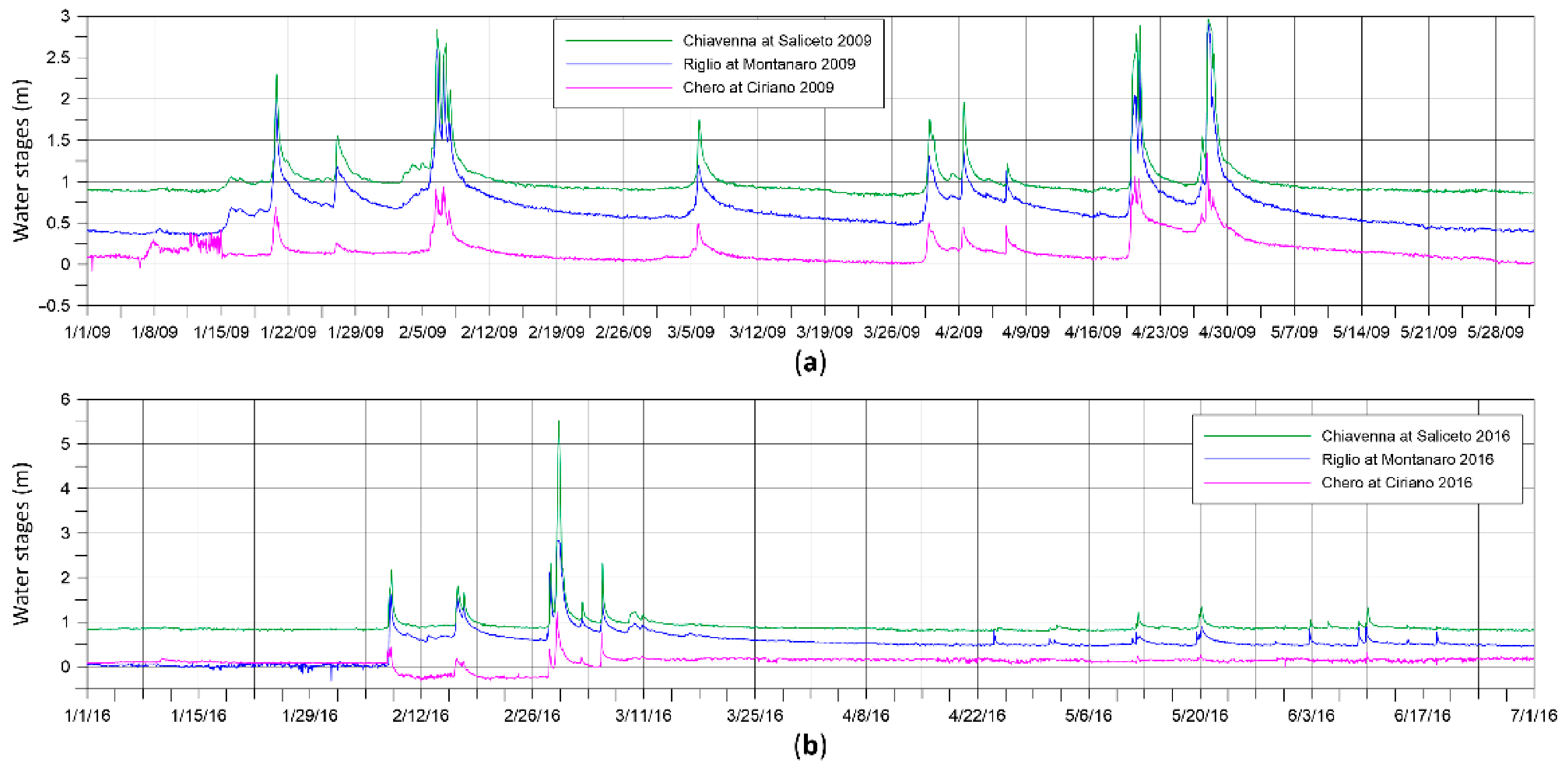
3.3.3. Water Stage Record Behavior

Riglio, Chero, and Chiavenna streams are usually subject to simultaneous floods. Negligible time lags between the peaks of the flood hydrographs, in the order of one to three hours, were, in fact, inferred by observing the historical water stage records (Figure 9). In the setting up of flooding scenarios, a synchronous behavior of the hydrological inputs will, therefore, be assumed.

4. Hydraulic Analysis

Hydraulic analyses focused on the hydrographic network, including the main reach of the Chiavenna stream and of the Chero and Riglio tributaries (Figure 10). The Riglio stream flows in a rather engraved riverbed and is provided with discontinuous embankments of modest height (1–2 m). The Chero stream has almost negligible embankments (<1 m) and runs through an alluvial plain characterized by a rather modest incision, unlike the Chiavenna, which flows upstream of Roveleto in a rather deep valley. The levee system of the Chiavenna stream originates at Roveleto and develops for about 10 km, with increasing height up to the confluence with the main Po River. All watercourses are crossed by several bridges.

4.1. Numerical Model

4.1.1. Hydraulic Model

The 2D hydraulic simulations were performed using the PARFLOOD code [37,39], developed at the University of Parma. This numerical model is based on an explicit finite volume discretization of the fully 2D shallow water equations (SWEs) [56], expressed using the well-balanced formulation proposed by [57]. The model is second-order accurate in both time and space, thanks to the adoption of the second-order Runge–Kutta method and of a depth-positive MUSCL extrapolation, while fluxes are evaluated using the HLLC approximate Riemann solver [56]. The model is compatible with both Cartesian grids and structured nonuniform grids, named Block-Uniform Quadtree (BUQ), as detailed in [37]. The adoption of an unevenly distributed spatial resolution is useful for reducing the number of computational cells in the domain and, consequently, the computational burden, while ensuring high accuracy in the areas of greatest interest (e.g., rivers, channels, buildings, hydraulic structures, embankments). Moreover, the code is developed in the compute unified device architecture (CUDA) environment, which enables parallel computing on graphics processing units (GPUs), leading to a drastic reduction in runtimes (of about two orders of magnitude) compared to serial codes, even for domains of several million cells [39]. The good performances of the PARFLOOD model in both simulations of theoretical cases and practical applications over complex bathymetries are well documented in previous works [11,34,58,59,60,61,62], to which the reader is referred for further details.

4.1.2. Bridge Modeling

Among the approaches available for the inclusion of bridges and other hydraulic structures in the 2D numerical models, internal boundary conditions (IBC) were favored in PARFLOOD thanks not only to their applicability to different flow conditions and structure types, but also to their suitability to predict the field-scale backwater effects induced by the fluid/structure interaction in case of high flows.

The IBC implementation is described in detail by [44] and, here, only very briefly recalled. In summary, each bridge is represented as a segment in the plane, which separates “upstream” and “downstream” IBC cells. The average water levels upstream and downstream of the bridge are computed over these cells, and then used to identify the current flow condition (free-surface flow, partially or fully pressurized flow, overtopping, Figure 11). If levels are below the bridge deck, the IBCs are not activated and only the bridge pier obstructions are considered. Otherwise, the discharge flowing through the structure is evaluated using available formulae from the literature [63] and imposed as specific discharge values at upstream IBC cells (redistributed according to the area available to flow). The same values are imposed in the corresponding downstream IBC cells, while water surface elevations are not modified, so that mass conservation is not impaired. Finally, the special flux treatment adopted at the edges between upstream and downstream IBC cells allows the bridge discontinuity to be naturally taken into account. An example of the application of IBCs to bridges in urban flood modeling is reported in [61].

4.2. Model Setup

4.2.1. DTM and Building Treatment

The study area covers over 180 km². A recent LiDAR survey provided a digital terrain model (DTM) with a resolution of 1 m × 1 m, which was converted to a raster map with a grid size of 2 m × 2 m, considered adequate for this test case. In the grid coarsening process, particular attention was paid to preserving the elevation of retaining structures along the streams and other thin linear topographic features in the domain. A further preprocessing of the DTM was necessary to restore the embankment crest elevations that were not correctly described due to the removal of the bank vegetation cover from the raw LiDAR data, and to integrate in the DTM the bathymetric portion of the riverbed not correctly detected due to the presence of water at the time of the survey.

The presence of buildings in urban areas was included by adopting the building hole (BH) approach [64]. This strategy requires that the computational cells falling within the footprints of buildings are removed from the mesh, which may be achieved by superimposing the shapefile containing the outlines of buildings on the DTM. Such a detailed building treatment is possible thanks to the high mesh resolution. Moreover, a total number of 21 bridges (Figure 12) were introduced in the hydraulic model.

4.2.2. Mesh

Starting from the DTM at 2 m × 2 m, a multiresolution grid with cells of variable size, from a minimum value of 2 m to the maximum of 2⁴ = 16 m, was built. In order to model the flood propagation accurately, all the main waterways, urban areas, and road and rail communication routes were described with the highest resolution (Figure 13). Elsewhere, the spatial resolution is automatically relaxed by the preprocessing algorithm, as described in [37]. The calculation grid thus identified is made up of a total of 6.8 million cells.

4.2.3. Domain Roughness

For the river beds, in the absence of data for calibration, a value of the Strickler’s roughness coefficient of 25 m^1/3 s⁻¹ was assumed based on local inspections, literature suggestions [65], and previous studies conducted by the authors concerning neighboring watersheds with similar characteristics [62]. Moreover, this value allowed the reproduction of, at best, the numerical rating curve previously obtained at Saliceto through 1D hydraulic modeling.

For the flooded areas, data for the calibration of roughness are usually unavailable. In literature applications, values for rural areas are highly variable, covering a range between 10 and 40 m^1/3 s⁻¹ [66,67,68,69]. For the low plain areas of Emilia-Romagna, indications can be obtained from the work by [34], where a Strickler’s coefficient equal to 20 m^1/3 s⁻¹ was calibrated to reproduce the well-known dynamics of the inundation caused by an embankment breach. Preliminary simulations of the present study indicated no significant differences in maximum water depths if values equal to 20 or 25 m^1/3 s⁻¹ were adopted outside the riverbeds, while flooding propagation times are slightly more influenced. As far as the time of arrival of the flooding is important in the emergency management phase during a real event, it is completely irrelevant for the identification of potentially floodable areas. In the absence of further information, it was, therefore, decided to adopt a uniform Strickler’s coefficient equal to 25 m^1/3 s⁻¹ over the whole domain.

4.2.4. Boundary and Initial Conditions

The SDHs obtained through the hydrological analysis were imposed as upstream boundary conditions at the sections indicated in Figure 12. At the confluence of the Chiavenna with the Po River, a constant water level was imposed as a downstream boundary condition, due to the presence of a power plant on the Po River just two kilometers downstream of the confluence. The water level upstream of the barrage of the power plant is constantly kept at 41.00 m a.s.l. [70], except for very high floods on the Po River, which never occur simultaneously with the floods of the Chiavenna stream, due to the enormous difference in size of the two river basins.

A steady flow of 10, 15, and 20 m³ s⁻¹ for the Chero, Chiavenna, and Riglio streams, respectively, was assumed as the initial condition.

5. Results

Four flooding scenarios were considered, adopting as inflow boundary conditions the synthetic design hydrographs estimated for T = 20, 50, 200, and 500 years. For the sake of space, only the main results of the study related to the T = 200 years reference scenario (the current flood protection standard in Italy) are presented here and discussed in detail. For this reference scenario, an additional corresponding simulation in the absence of all bridges was performed, in order to evaluate the obstruction effect exerted by these structures. The comparison between the numerical results in the presence and absence of bridges allows an immediate assessment of their influence on the flooding dynamics and on the extent of the flooding upstream and downstream of the urban area of Roveleto.

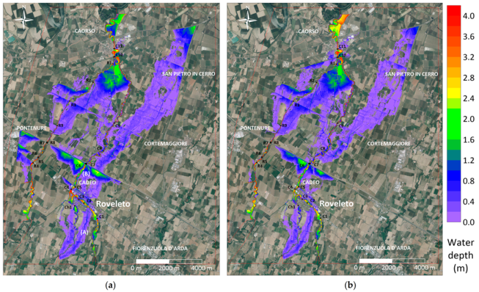
For the 200 years scenario in the current state, the extension of the flooded areas is remarkable (Figure 14a). Flooding due to the insufficient conveyance of the Chero extends downstream, reaching Roveleto and partly reflowing into the Chiavenna stream (A in Figure 14a). The flooding involves almost the entire town of Roveleto, where pressurized flow is observed at all the bridges, some of which are also overtopped, albeit to a modest extent. The flooded waters also lean against the railway embankment, which is largely overtopped. Proceeding northwards, the flooding extends further downstream, reaching the motorway and the high-speed railway (B in Figure 14a), with depths higher than 2 m. Both the infrastructures are overtopped, and the flooding spreads in the northeast direction towards San Pietro in Cerro and is retained by other motorway embankments. Additional inundations due to outflows from the Riglio stream are also observed, and the water depths are particularly high in the rural area bounded by the two streams, upstream of Caorso. Overall, the scenario is extremely severe in terms of flooded urban and suburban areas and of the crucial transport infrastructures involved.

The same hydrological scenario has been simulated in the hypothetical situation of the absence of all bridges. In this case, a minor extension of the flooding and lower water depths occurs in the areas upstream of the removed crossing structures. At the same time, larger flooding areas are estimated downstream due to the higher discharge released, which exceeds, to a greater extent, the conveyance of the downstream river branches (Figure 14b).

The differences in the flooding extent are even more evident if we focus on the urban area. Figure 15a shows the detail inside Roveleto in the current state, showing that urban areas are totally flooded due to the backwater effect induced by the presence of crossing structures with insufficient conveyance. With reference to the northernmost portion of the inhabited area between the two streams, close to the confluence, the water depths on the ground are still quite low (less than 0.6 m, waterways and underpasses excluded). However, it should be noted that the presence of even a few tens of centimeters on the ground necessarily implies the total flooding of the underground floors, a circumstance that is not immediately evident due to the lack of description of these elements in the DTM.

Even in the hypothetical scenario of absence of all the bridges, the majority of the urban area of Roveleto is flooded, but with almost halved water depths compared to the current situation. The reduction in the maximum levels, of the order of several tens of centimeters, would result in a significant reduction in the areas involved, preserving more than half of the urban area from flooding. From Figure 15b, it can be appreciated that the portion of Roveleto, bounded by the Chero and the Chiavenna immediately upstream of their confluence, would be almost entirely unaffected by the flooding. It then follows that, even if the railway is still overtopped, the flooding spreading towards the northeast involves a smaller area. This is obviously due to the lower level of the flooding originating upstream of the highway as a result of the free outflow at the section of the bridge (here removed). The overtopping of the embankments of the highway and of the high-speed railway would be, in this case, minimal. In the absence of bridges, the decrease in maximum water levels ranges from a few tens of centimeters up to one meter and more, with an extreme benefit in terms of population and assets involved. However, the solution of rebuilding the majority of the bridges, increasing their deck level and removing abutments (situation similar to this hypothetical scenario), does not appear to be easily achievable due to the elevation constraints induced by the existing main infrastructures, such as roads, motorways, and railways. Moreover, the removal of the crossing structures, due to the consequent absence of the obstruction effect, allows greater discharges to propagate downstream, giving rise to an increase in water levels in the lower stretch of the stream compared to the current situation, possibly inducing additional outflows. For this reason, the rebuilding of the bridges, besides being difficult to implement, does not even seem appropriate to secure the entire territory from the risk of flooding.

Bridges’ Conveyance

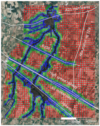
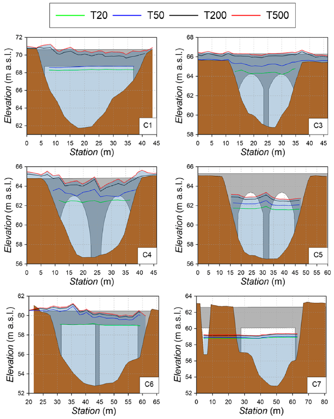
Figure 16 shows a few examples of the maximum water levels upstream of six of the more than twenty bridges present in the computational domain (see Figure 12 and Figure 14 for their location).

It is worth noting that each profile does not refer to a particular instant, but represents the envelope of all the results obtained during each transient simulation, possibly including flooding outside of the river (see bridge C4 for the 200- and 500-years scenarios). For the most upstream bridges, incipient (C1) or weak (C3) pressurization is already estimated for the T = 20 years scenario. The conditions become slightly less severe further downstream (C4) due to the reduced discharge caused by the upstream flooding. For T = 50 years, complete pressurization conditions are estimated at the bridges inside Roveleto (C1, C3, and C4). Free outflow instead occurs from the railway crossing onwards (C5, C7), with few exceptions (C6). For the scenario with return period T = 200 years, for all bridges inside Roveleto, pressurization and incipient overflow conditions occur. Again, free outflow is observed along the Chiavenna from the railway onwards, with the exception of the motorway bridge that is slightly overtopped on the left side (C6). With reference to the catastrophic scenario for T = 500 years, a general worsening of the outflow conditions inside Roveleto is observed. Free outflow is still observed along the Chiavenna at the railway crossing, while the outflow conditions at the bridges further downstream worsen appreciably.

6. Discussion and Conclusions

The case study analyzed here can be considered a reference example of the many challenges faced in hydrologic/hydraulic flood hazard modeling when dealing with poorly gauged watersheds. In this work, some improvements in already consolidated literature methodologies are introduced as regards the hydrologic analysis, while a recently proposed approach for bridge inclusion in fully 2D hydrodynamic models solving the complete SWEs is applied for the first time, with the purpose of assessing the adequacy of bridge conveyance in a complex urban environment.

As regards the hydrologic analysis, due to the scarcity of reliable field observations, the flooding scenarios simulated for different return periods were conducted with reference to synthetic design hydrographs, the peak discharges of which were estimated through a regional approach. Of course, this procedure can lead to results affected by an uncertainty that is difficult to quantify. Nevertheless, the choice to rely on estimates based on regional procedures seems appropriate and promising. Recent studies have, in fact, shown that, in this region, the methodologies adopted for the estimation of the discharge quantiles are characterized by a good reliability [47]. It will be very important in the future to deepen the analyses at a regional scale by expanding the database of direct observations of the reference hydrological variables as much as possible. Some difficulties arising in the fitting of the empirical reduction ratios through the well-known Equation (6) suggested adopting a generalized form of the same relation, in which the presence of an additional parameter allowed a better fit for the available observed values. Moreover, the possibility of deriving the reduction factor on the basis of the analysis of water stages (therefore, not relying on the stage–discharge conversion) could dramatically increase the set of observations available for regional analyses. This would make it possible to exploit historical information available at gauging stations devoid of reliable rating curves, but sometimes rich in several decades of reliable hydrometric water stage records instead. Large-scale analyses that cannot be undertaken at the present time since, in the vast majority of watersheds, only a small percentage of gauging stations is equipped with a reliable stage–discharge relationship would, therefore, be allowed. Both of these aspects seem to be worthy of further investigation.

As regards hydrodynamic modeling, all flooding scenarios are simulated here adopting a GPU-parallelized model based on an explicit shock-capturing finite volume method for the solution of the fully 2D shallow water equations. The river and the flood-prone areas belong to a unique computational domain, and the flow is modeled avoiding the special treatments required by other simplified numerical schemes (quasi 2D, 1D–2D, etc. [71]). Moreover, the hydraulic modeling of the many bridges present in the flow field is here conducted following a truly 2D approach. This prevents significant flow field distortions that can occur in case contiguous crossing structures are modeled following too simplified approaches. Thanks to an efficient parallelization, the issues related to long computational times are overcome, even in the case of high-resolution grids and even when a very large number of crossing structures are introduced. This is of great importance since preserving computational efficiency without affecting the accuracy of the description of the interfering elements is a fundamental objective to lay the foundations for an increasingly advanced ultra-fast modeling that allows real-time detailed simulation to be achieved in the near future.

The strategy of comparing flooding scenarios with and without bridges is used here to investigate possible structural measures to reduce the flood hazard in the study area, e.g., the rebuilding of bridges with increased deck elevation and in the absence of abutments. Indeed, it is evident that most of the bridges are inadequate to convey floods with large return periods. In the absence of bridges, the reduced backwater upstream of the crossing structures would result in a significant decrease in the inundated areas, preserving from flooding at least half of the inhabited center of Roveleto. However, this solution does not appear to be easily practicable due to the elevation constraints induced by the existing infrastructures, roads, and railways. Furthermore, this intervention would not be sufficient to prevent the urban inundation completely, and does not even appear entirely desirable, given the proven worsening of the downstream conditions due to the greater discharge released. Therefore, further structural interventions have to be designed, and the high-resolution 2D model setup for this study can be an extremely powerful tool for assessing the effectiveness of any adaptation measure to reduce the exposure to flood of Roveleto without increasing flood hazard in downstream territories. Examples may include the local adjustments of the embankments’ elevations or the identification of temporarily floodable areas upstream of the urban center.

In summary, the flood hazard assessment conducted here with reference to a poorly instrumented watershed has highlighted how the use of an integrated approach of hydrological and hydraulic methodologies can lead to results useful for the design of infrastructures and civil protection purposes. The methodology proposes a series of good practices that can also be applied in those circumstances in which the essential assessment of the flood hazard in highly urbanized areas may, at a first glance, appear strongly discouraged by the scarcity of reliable local hydrological information.