Estimation of Peak Discharges under Different Rainfall Depth–Duration–Frequency Formulations

Abstract

One of the main signatures of short duration storms is given by Depth–Duration–Frequency (DDF) curves. In order to provide reliable estimates for small river basins or urban catchments, generally characterized by short concentration times, in this study the performances of different DDF curves proposed in literature are described and compared, in order to provide insights on the selection of the best approach in design practice, with particular reference to short durations. With this aim, 28 monitoring stations with time series of annual maximum rainfall depth characterized by sample size greater than 20 were selected in the Northern part of the Puglia region (South-Eastern Italy). In order to test the effect of the investigated DDF curves in reproducing the design peak discharge corresponding to an observed expected rainfall event, the Soil Conservation (SCS) curve number (CN) approach is exploited, generating peak discharges according to different selected combinations of the main parameters that control the critical rainfall duration. Results confirm the good reliability of the DDF curves with three parameters to adapt on short events both in terms of rainfall depth and in terms of peak discharge and, in particular, for durations up to 30 min, the three-parameter DDF curves always perform better than the two-parameter DDF.

1. Introduction

The investigations about the increasing of extreme events at a global level carried out in last decades generated a debate on the need of revisiting the risk management approach, in particular with regard to rainstorms and floods. Concerns and possible consequences deriving from changes in an extreme rainfall regime led scientists and practitioners to investigate the influence of these events on the current design practice. One of the most used tools in water management are the Depth–Duration–Frequency (DDF) and Intensity–Duration–Frequency (IDF) curves, which have the valuable quality of being analytical relationships able to provide a design rainfall depth (or intensity) for an assigned duration and return period [1,2]. The underlying theoretical framework of these curves has been widely discussed and assessed in hydrological literature (e.g., [2,3,4,5,6]). However, concerns about past changes and possible evolutions of climate on the phenomenology of rainfall raised questioning about the opportunity of retaining the still valid adoption of stationary hypothesis during the IDF/DDF deriving procedure [7,8,9,10]. Implications arising from the adoption of nonstationary probability distributions for modelling changes in extremes and applications of related statistical tests for trend detection were discussed in several studies (e.g., [11,12,13,14,15,16,17,18]).

Starting from the middle of the 20th century, the first relationships between depth (or intensity) and duration of rainfall were studied above all in developed countries such as the USA, the UK and Ireland [19]. The results of these analyses can be applied in water resources engineering for the mitigation of hydraulic risk and are particularly needed for urban areas with poorly permeable surfaces and small catchment and, consequently, very short run-off times. Typically, two- or three-parameter DDF/IDF formulations are considered in design practice [5], in a balance between an enhanced model structure and parameter uncertainty [2]. Obtaining analytical results that are compatible for reliable design purposes, requires the availability of recorded time series for durations critical of the same order of magnitude of physical processes having place in the environment. As in the case of urban basins and small catchments, often mass transfer phenomena require durations less than 1 h, making essential the availability of rainfall series which span this time domain [3]. These data were very difficult to retrieve in the past, but refinements in recording technology together with new technologies (such as satellite and radar observations) are providing scientists and practitioners with new updated and consistent datasets of data. However, it should be noted that databases of rainfall time series in short durations (5, 15 and 30 min) are generally less extensive than hourly data. In this sense, short-duration rainfall data constitute a precious source of information for investigating if remodulation in the extreme rainfall regime is happening, and their use in the context of a test for trend detection (and the consequent adoption of a nonstationary probabilistic model) may deserve particular attention, because the low magnitude of the trend and the reduced sample size of recorded data may lead to low power statistical tests [14,15].

Disregarding the stationary/nonstationary problem (whose discussion is outside the aim of this paper), as remarked before, the increased availability of short-duration series constitutes an important support for building DDF/IDF curves that are more consistent with observed data and for improving design operations, often based on the classical two-parameter ‘Montana curve’. With respect to Italian case studies, we mention the work of Di Baldassarre et al. [2] (Emilia Romagna and Marche regions) and of Rossi and Villani [20] (Campania region), where DDF curves with more than two parameters were applied.

The study of short storm durations that extend from a few minutes to an hour is interesting for several design purposes. They may trigger flash floods characterized by short durations and occurring on small catchments such as a part of cities such as residential areas or infrastructures. Design practice often leads to the need to define drainage and disposal systems for rainwater for small drainage surfaces intended for urban, commercial or industrial use. Therefore, the small size of the drainage area in addition to the low permeability of the soil, may produce hydrological responses characterized by short lag times, with a preponderant runoff with respect to the infiltration component. Furthermore, often rainfall and discharge observations are not available, addressing the practitioner to apply empirical approaches [21].

With the aim of providing a quantitative discussion on the influence of different DDF formulations on the evaluation of peak discharges, an extended analysis is conducted exploiting the widely used SCS-CN method (e.g., [22,23]), in order to test the ability of different DDF/IDF curves in reproducing the peak discharge corresponding to an observed rainfall event. In the SCS-CN method, the critical rainfall duration depends on three parameters: the catchment area, basin slope and CN. The application to urban basins is carried out through the choice of a parameters range, i.e., high values of the CN from 50 to 100, small areas from 0.1 to 10 km² and an average slope of the basin from 3% to 18%. For each combination of these parameter values, the corresponding concentration time is calculated using the SCS-CN method. After obtaining the concentration time values, the peak discharge is calculated with the observed rainfall depth compared with those obtained from different DDF formulations.

Furthermore, peak flow curves based on a sensitivity analysis were created to compare results obtained from the two-parameter and three-parameter DDF curves. The study also provides an evaluation of the relative error of DDF on peak discharge, highlighting the benefits of the use of three-parameter DDF curves in practical applications.

The paper is structured as follows: In Section 2 the case study of Northern Puglia (South-Eastern Italy) and dataset consistence are illustrated, while in Section 3, DDF and IDF curves used for the analysis are described, including steps for the evaluation of peak discharge obtained from the corresponding DDF curves and estimated by means of the SCS-CN method. In Section 4, results of illustrated applications are critically discussed and in Section 5 conclusions are reported.

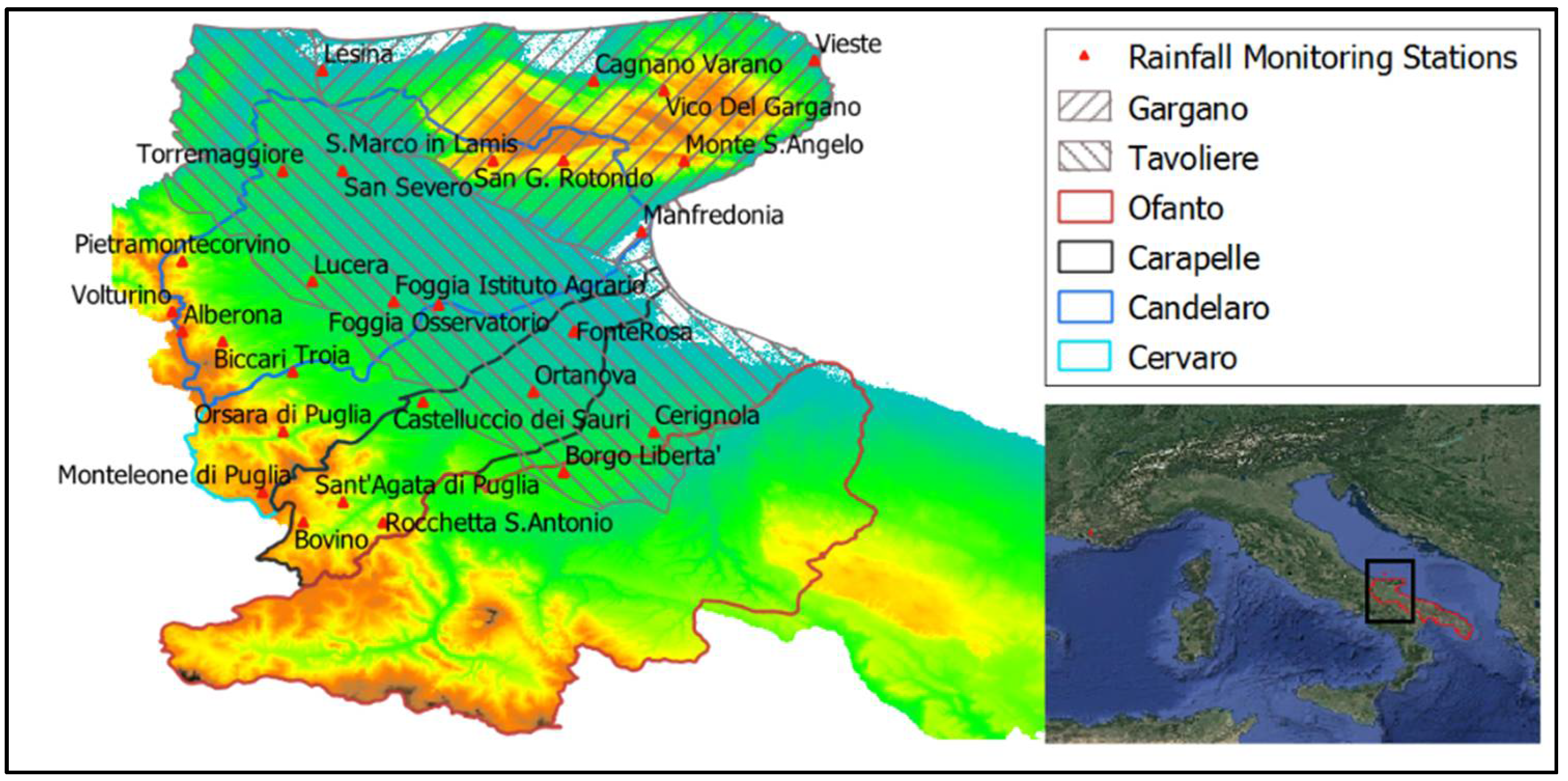
2. Study Area and Dataset

Puglia is the region of peninsular Italy with the greatest coastal development and its territory is covered by 1.5% of mountains, 45.2% by hills and 53.3% by plains. The study area is located in the northern part of the Puglia region (Southern Italy) and, moving from South-West to North-East, is constituted by the Daunian Apennine, the Tavoliere plain and the Gargano promontory (Figure 1). The highest peak of the Daunian Mountains is Monte Cornacchia (1151 m a.s.l.) and is located on the border with the Campania region, followed by the 1055 m high Monte Calvo in the Gargano promontory.

The most important rivers inside and surrounding the study area are Fortore, Candelaro, Carapelle, Cervaro and Ofanto, whose main streams cross or delimit the Tavoliere plain. Due to the steep change in slope, from mountains to the plain, the regime of rivers in the area is torrential, and urban areas are prone to flash floods that may be triggered by frontal events, convective storms or Mediterranean cyclones [24,25]. Moreover, low-lying coastal areas are often affected by inundation phenomena due to the combined effect of heavy rainfalls and severe storm surges [26].

The analyses were carried out exploiting rainfall data recorded by a gauges network managed by the Civil Protection of Puglia Region. For this study, annual maximum series with a duration of 5, 15 and 30 min and 1, 3, 6, 12 and 24 h were employed, with a recording period comprised between 1921 and 2019. Data are freely available and can be downloaded by accessing the website of the Civil Protection of Puglia Region [27]. In order to provide more reliable evaluations, only stations with time series greater than 20 data for all durations were selected. In Figure 1, positions of selected stations in the study area are illustrated, while in

Table 1. Rainfall monitoring stations.

Rainfall Monitoring Stations	Altitude (m a.s.l.)	River Basin/Area	Installation Year
Alberona	663	Candelaro	1917
Biccari	484	Candelaro	1922
Borgo Liberta’	235	Ofanto	1924
Bovino	623	Carapelle	1917
Cagnano Varano	165	Gargano	1921
Castelluccio dei Sauri	190	Carapelle	1922
Cerignola	118	Tavoliere	1921
Foggia Osservatorio	99	Candelaro	1873
Foggia Istituto Agrario	85	Candelaro	1949
Fonte Rosa	25	Tavoliere	1925
Lesina	6	Gargano	1928
Lucera	246	Candelaro	1917
Manfredonia	68	Tavoliere	1900
Monte Sant’Angelo	799	Gargano	1920
Monteleone di Puglia	828	Cervaro	1920
Orsara di Puglia	689	Cervaro	1921
Ortanova	53	Carapelle-Tavoliere	1921
Pietramontecorvino	441	Candelaro	1928
Rocchetta Sant’Antonio	724	Carapelle	1922
Sant’Agata di Puglia	703	Carapelle	1917
San Giovanni Rotondo	619	Candelaro-Gargano	1923
San Marco in Lamis	566	Candelaro-Gargano	1917
San Severo	114	Candelaro-Tavoliere	1928
Torremaggiore	195	Candelaro-Tavoliere	1917
Troia	469	Candelaro	1907
Vico Del Gargano	459	Gargano	1921
Vieste	96	Gargano	1921
Volturino	615	Candelaro	1964

their main characteristics are reported.

3. Methodology

3.1. Formulations of DDF/IDF Curves

As recalled in the Introduction, several formulations have been used for characterizing DDF/IDF relationships. Following Di Baldassarre et al. [2], we limited our analysis to the DDF with two and three parameters, considering the consistency of the available dataset inadequate for other formulations.

Among two-parameter DDF curves, we focused our attention on the following:

$$h=a{d}^b$$

(1)

Known also as ‘Montana curve’, Equation (1) expresses the rainfall depth h (mm) by means of a power law of storm duration d (h), using parameters a and b. Despite its simplicity, it can be considered the standard relationship implemented when approaching the problem of DDF estimation. However, several criticisms have been moved to this formulation. Turning to the intensity i, defined as the ratio between the rainfall depth h and its duration, this value goes to infinity when the duration d of the event approaches to zero [2]. In the context of the two-parameter formulation, starting from Equation (1), two specific case studies were identified for the purposes of this work: in the first, we indicated with D2P-1 Equation (1) when parameters a and b were estimated considering both the hourly and sub-hourly data, while in the second case, we indicated with D2P-2 Equation (1) when parameters a and b were estimated considering only the hourly data. This choice was motivated by the need of providing a comparison with the practice of using hourly data, widely diffused in the real world due to the limited amount of short-duration rainfall data diffused in the past decades.

In the realm of three-parameter formulations, the following DDF equations were analyzed starting from the available datasets, respectively, called D3P-1, D3P-2 and D3P-3:

$$\mathrm{h}=\frac{ad}{{\left(d+c\right)}^b}$$

(2)

$$\mathrm{h}=\frac{ad}{\left(d^b+c\right)}$$

(3)

$$\mathrm{h}=\left(c+\frac{a}{d+b}\right)d$$

(4)

with a, b and c parameters to be estimated. All parameters of DDFs were estimated by using the least squares technique. Equations (2)–(4) are the same formulations of DDF with three parameters investigated in Di Baldassarre et al. [2]; our choice was also motivated by the opportunity of having a similar investigation of a geographically similar area, which ranges from the Apennine chain to the Adriatic Sea.

3.2. Error Measures

Stands that $h=h\left(d\right)$, a quantitative evaluation of the goodness of estimate of rainfall depth $h_j$ obtained using each of the selected DDF curves in comparison with the observed average rainfall depth $\overline{h_j}$ was carried out for all the $j=1,2,\dots ,N$ monitoring stations and for all $i=1,2,\dots ,M$ durations of recorded event. Analysis is performed by applying: (i) the relative error ${\epsilon }_j\left(d_i\right)$ for each monitoring rainfall station and duration; (ii) the mean absolute percentage error $E\%$ calculated for each duration and averaged over all the monitoring rainfall stations and (iii) the Root Mean Square Error (RMSE), integrated over all the durations and monitoring station. In particular, the observed rainfall depth $\overline{h_j}$ was evaluated considering the average value on the time series for each duration and for each monitoring station. The evaluation of these error indicators represents a reliability test as also analyzed in Di Baldassarre et al. [2], but, in this case, was considered independent from the return period. The relationships was hereafter reported:

$${\mathbf{\epsilon }}_j\left(d_i\right)=\frac{h_j\left(d_i\right)-\overline{h_j}\left(d_i\right)}{\overline{h_j}\left(d_i\right)}$$

(5)

$$E \left(d_i\right)\%=\frac{100}{N}·{\displaystyle \sum }_{j=1}^N\frac{\left|h_j\left(d_i\right)-\overline{h_j}\left(d_i\right)\right|}{\overline{h}\left(d_i\right)}$$

(6)

$$RMSE=\frac{1}{M}·{\displaystyle \sum }_{i=1}^M\sqrt{{\displaystyle \sum }_{j=1}^N\frac{{\left[h_j\left(d_i\right)-\overline{h_j}\left(d_i\right)\right]}^2}{N}}$$

(7)

3.3. SCS-CN Method

In order to test the effect of the investigated DDF/IDF curves in reproducing the design peak discharge corresponding to an observed rainfall event, the Soil Conservation (SCS) curve number (CN) method was applied. The SCS-CN is a conceptual method, widely used in many hydrologic applications for predicting runoff from watersheds. The first publication of SCS-CN method dates back to 1956 and was proposed by the U.S. Department of Agriculture in the National Engineering Handbook of Soil Conservation Service [23]. This method was originally elaborated to predict runoff volumes for a given rainfall event and for the evaluation of storm runoff in small agricultural watersheds [28]. Rallison [22] describes the origin and development of SCS method, based on infiltrometer tests and measures of rainfall and runoff. The SCS-CN method was developed well beyond its original scope and was adopted for different land uses and climate conditions [29,30,31,32,33,34,35,36]. This approach has been taken as procedure by many users (professionals or public administrations) in numerous hydrological applications for design flood estimation and/or for runoff evaluation for a particular storm event (e.g., [37]). More details about the theoretical background are given in Pilgrim et al. [38].

The peak discharge was computed using a triangular hydrograph method developed by Mockus [39] and reported in Pilgrim et al. [38], with rainfall characterized by duration equal to D. Considering the definition of lag time, t_l (distance between the centroid of excess precipitation and the peak of the hydrograph) provided by the Natural Resource Conservation Service (NRCS, [40]), the peak discharge, q_p, was reached in a duration T_P (i.e., time of rise).

Application of SCS-CN Method

In order to test the performances of the three-parameter DDF curves, in this work, the SCS-CN method was used for calculating the runoff volume and the triangular hydrograph method for evaluating the expected value of peak discharge, using both the three three-parameter and the two classic two-parameter expected DDF curves described in Section 3.1. In this way, according to Equation (8), the evaluation of peak discharge depended on the rainfall volume, V, drainage basin area, A, and lag-time$, t_l$; according to Equation (10), lag time $t_l$ depends on the mainstream length, L, the river basin’s slope, s, and the Curve Number, CN.

The peak discharge q_p (m³/s) is given by:

$$q_p=\frac{0.208AV}{0.5D+t_l}$$

(8)

A (km²) is the area of the drainage basin and V (mm) is the depth of runoff.

Assuming D equal to a concentration time and considering the empirical relationship between the concentration time and lag-time proposed by Ward and Elliot [41]:

$$D=t_c=t_l/0.6$$

(9)

$$t_l=0.342\frac{L^{0.8}}{s^{0.5}}{\left(\frac{1000}{CN}-9\right)}^{0.7}$$

(10)

L is connected to basin area through an empirical equation introduced by Hack [42] and hereafter reported:

$$L=1.4 A^{0.6}$$

(11)

This relation was also discussed in recent scientific literature such as Maritan [43] and Rinaldo [44].

Different combinations of parameter values A, s and CN were selected (considering usually observed ranges in small river basin) leading to the definition of different lag time values, according to Equation (10) and, consequently, rainfall durations (D), assumed equal to the concentration time t_c. Thus, for each selected duration, in according to Equation (9), the expected rainfall depth, evaluated through the D2P-1, D2P-2, D3P-1, D3P-2 and D3P-3 curves, was used for calculating the runoff and, consequently, the expected peak discharge$, q_p$, according to Equation (8).

The different combinations of these parameters simulated the conditions of urban basin characterized by small area and high impermeability. For this reason, a basin area with range from 0.1 to 10 km², CN values from 50 to 100 and slope from 3% to 18% were chosen.

4. Results and Discussion

For each of the 28 investigated rainfall monitoring stations, all DDF/IDF formulations described in Section 3.1 were fitted. Results are shown in graphical form in Figure 2. only for six rainfall monitoring stations selected, each falling within a basin or zone of the study area. The curves D2P-1, D2P-2, D3P-1, D3P-2 and D3P-3 were plotted on the left side of each subplot, in addition to the observed (mean) values of rainfall depth for all durations; in the right part of the subplots, the relative IDF curves (I2P-1, I2P-2, I3P-1, I3P-2 and I3P-3) are shown on the basis of the estimated parameters of the corresponding DDF curves.

Focusing on the short durations from 5 min to 1 h, the intensity evaluated using three-parameter DDF curves was lower and more reasonable than that obtained with two-parameter DDF curves, as shown in Figure 3. Additionally, in this case, shown only are the results of the same rainfall monitoring stations selected for the Figure 2.

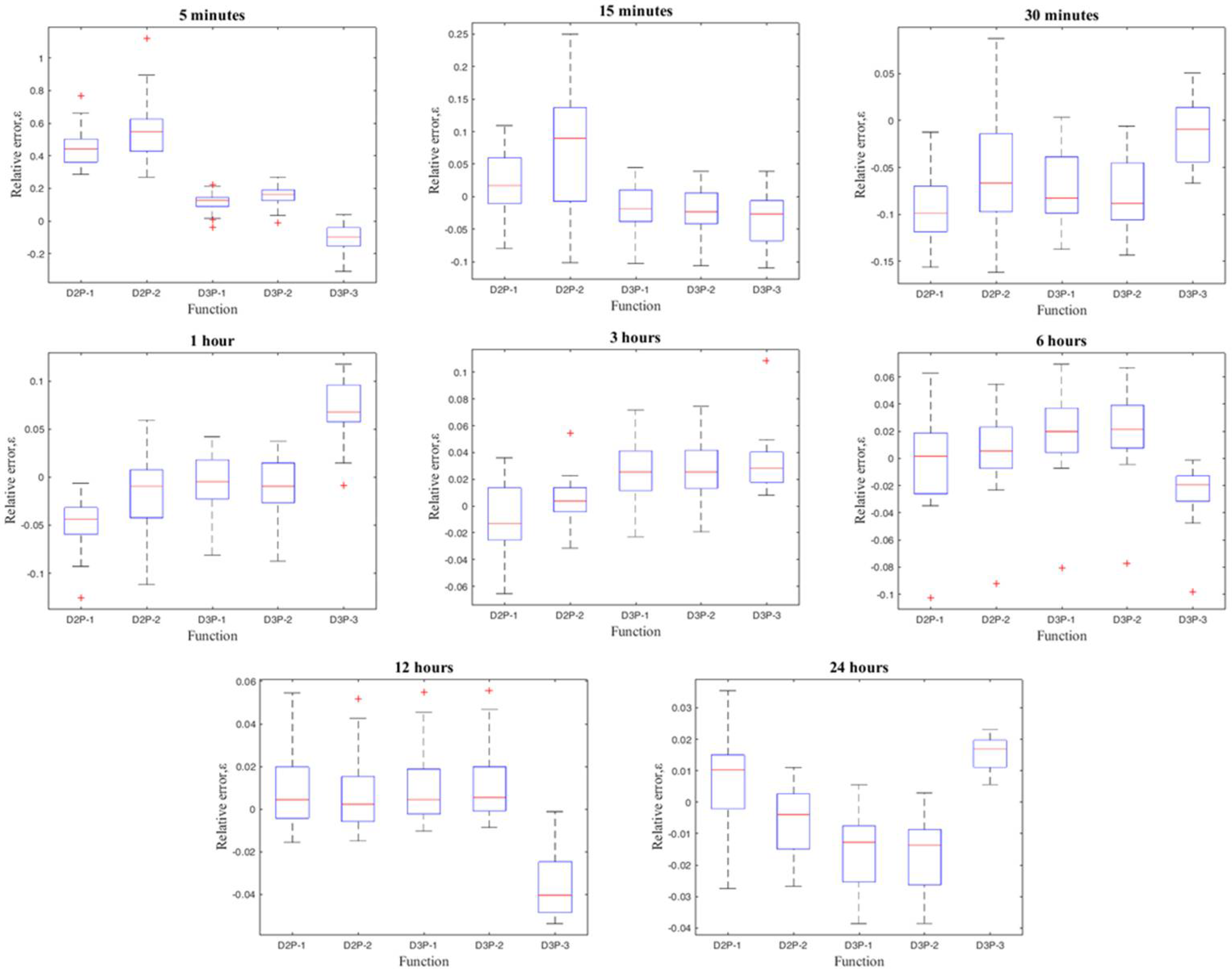
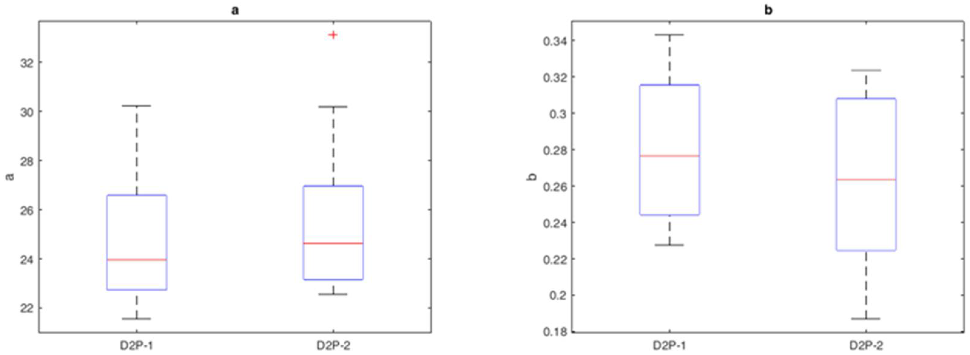
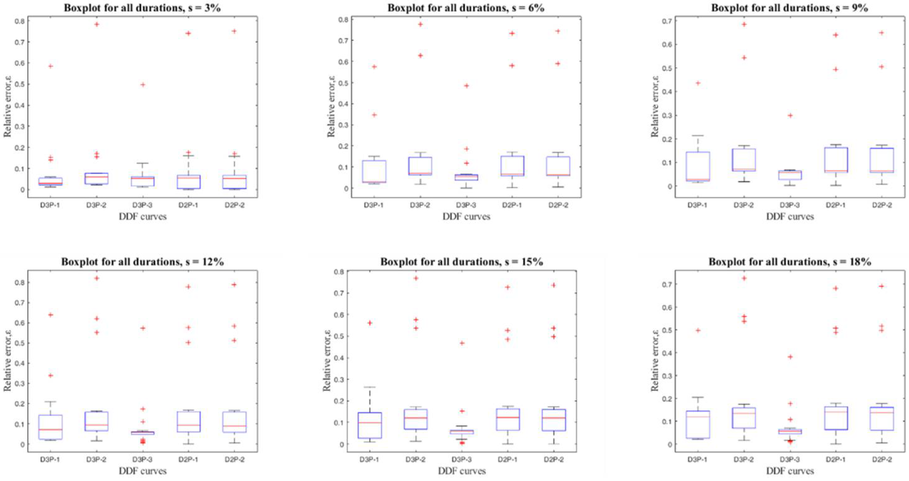
4.1. Results of DDFs Error Measures

In Figure 4, the box plots of the relative errors (with reference to all the investigated monitoring stations) for the considered DDF equations are reported. Focusing on the boxplot of D2P-1 and D2P-2, it was interesting to observe the poorer performance of the two-parameter curves for short durations; the worst, between them, was the D2P-2 equation, which presented a greater variability of the relative error, for short durations (5, 15 and 30 min). For durations equal to or greater than one hour, the D2P-2 showed less uncertainty than D2P-1. The comparison between D2P-1 and D2-P-2 was further explored through Figure 5. The three-parameter DDF curves seemed to have a far better performance than the two-parameter DDF curves especially for durations of 5 and 15 min.

Figure 5 shows the boxplot for the D2P-1 and D2P-2 parameters (a and b). The subplot on the left compares the parameter aestimated considering in the first case sub-hourly and hourly data and in the second case only hourly data; on the right the same comparison is shown for the parameterb. It is interesting to note that the estimated parameter, a, which represented the expected rainfall depth of duration equal to one hour, presented a higher uncertainty when estimated from a greater range of durations (i.e., including short durations). The parameter b had, in both cases, an extremely low variability.

The Mean Absolute Percentage Error $\left(\mathrm{E}\%\right)$ and the Root Mean Square error (RMSE) averaged over all the durations and the monitoring stations are, respectively, reported in

Table 2. Mean Absolute Percentage Error.

	D2P-1	D2P-2	D3P-1	D3P-2	D3P-3
E (d5)%	44.58	55.26	11.82	15.36	11.63
E (d15)%	4.40	9.54	3.11	3.21	3.99
E (d30)%	9.26	7.47	7.34	8.00	2.82
E (d60)%	4.76	3.03	2.26	2.43	7.17
E (d180)%	2.40	1.19	2.73	2.80	3.12
E (d360)%	2.15	1.87	2.57	2.67	2.38
E (d720)%	1.54	1.45	1.48	1.48	3.48
E (d1440)%	1.41	0.96	1.55	1.64	1.54

and

Table 3. Root Mean Square Error.

	D2P-1	D2P-2	D3P-1	D3P-2	D3P-3
RMSE	1.64	1.68	1.14	1.21	1.33

.

It is possible to note from Table 2, that the worst performance for durations of 5 and 15 min in terms of the mean absolute percentage error were given by D2P-2, followed by D2P-1, both characterized by two parameters. On the other hand, for rainfall events with durations greater than or equal to one hour, the performance of both D2Ps improved, while the D2P-2 remained the best performing DDF, among all. The better performance of DDF with three parameters which is visible in Table 3 in terms of RMSE, was mainly attributed to their better fit of short rainfall events.

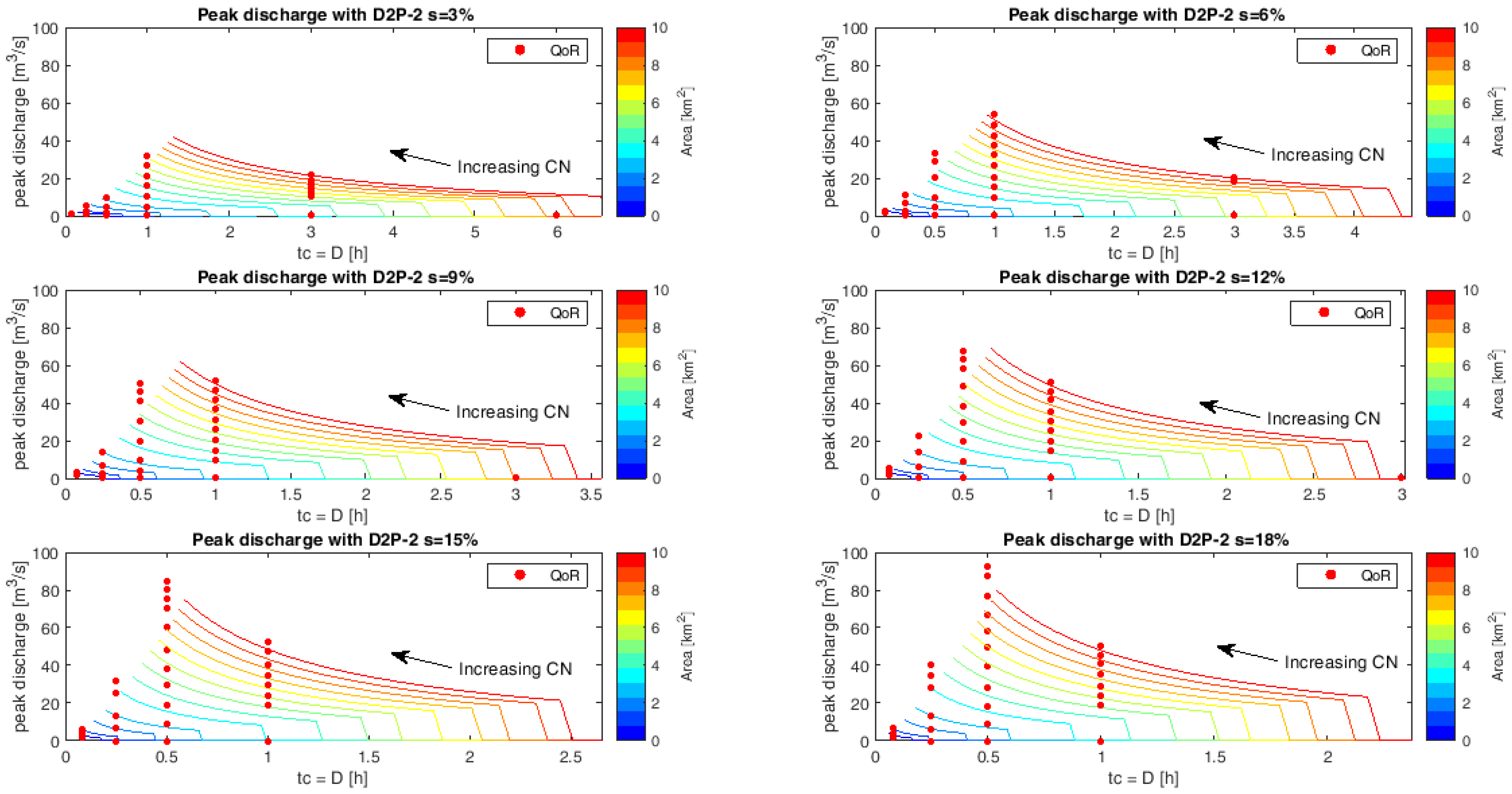
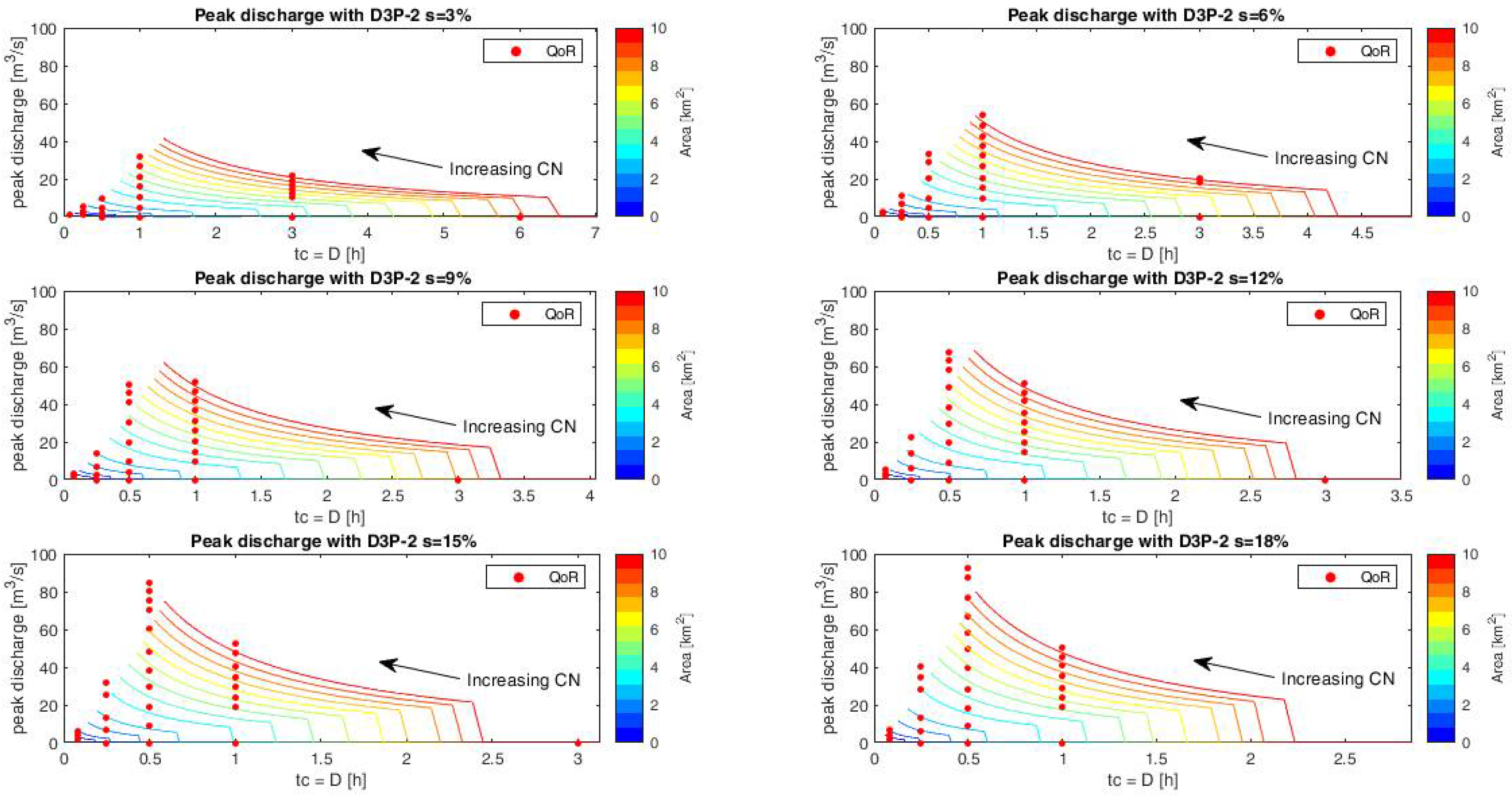
4.2. Results of Applications of SCS-CN Method

As previously explained, the application of the SCS-CN method was conducted for understanding the effect of DDF curves with three parameters on the expected peak discharge for short-duration rainfall events. All the monitoring stations were examined, but for the sake of brevity, only one example case was reported. In particular the results for the Alberona monitoring station are shown and the graphs were obtained as explained in Section 3.3. Figure 6, Figure 7, Figure 8, Figure 9 and Figure 10 report the peak discharge values, obtained using rainfall input from the DDF equations and different combinations of quantities A, s and CN on which the rainfall duration was set. As remarked before, the rainfall duration D was assumed equal to the concentration time t_c. Each figure, corresponding to a selected DDF curve was composed of six sub-plots which referred to different selected values of slope s. Each curve in the graph was obtained for a fixed drainage area, A, varying the CN value; in particular, according to Equations (9) and (10) the concentration time decreased with an increasing CN. The different curves reported in each subplot, were generated changing the catchment area; therefore, a curve beam was obtained where each color corresponded to a value visible in the legend of the plot. Red points, called QoR “Q-Peak evaluated with observed Rainfall”, represented the peak discharge values obtained, for each observed duration, by applying the same SCS-CN method for each combination of the three quantities (CN, A and s) and considering the gauged input rainfall volume. It was also necessary to observe that, for a chosen value of basin area and basin slope, a minimum concentration time was obtained corresponding to CN = 100.

Figure 6, Figure 7, Figure 8, Figure 9 and Figure 10 illustrate the results on peak discharge, for the case study of Alberona monitoring station, applying the SCS-CN method with different DDF curves highlighting the capability to adapt to the observed peak discharge, in particular for durations lower than one hour. The Figures highlight that, for short durations, a comparison was possible only for the basins with a high value of CN, and performances may depend significantly from the basin size and average slope. In general, these results confirmed the good reliability of the DDF curves with three parameters to adapt on short events, both in terms of rainfall depth and in terms of peak discharge.

To evaluate, in terms of error, the fit of the known curves to the QoR, the mean absolute percentage error was calculated on all the stations for the different slopes examined, focusing on the short durations (5, 15, 30 and 60 min). These results are shown in graphical form in Figure 11. The best fit corresponded to the least error and showed that, for durations up to 30 min, the three-parameter DDF curves always performed better than the two-parameter DDF curves. Among the three-parameter DDFs, the worst performance was given by D3P-2 with E% between 20% and 30%, while the best one was provided by the D3P-3 with errors always below 10%. Figure 11 also shows that there was a significant dependence on the slope of the basin in the calculation of the peak flow related to the lag time and, hence, on the propagation of the error from the rainfall input to the peak flow output. For durations equal to or greater than an hour, the best DDF curve may have changed with duration, looking both to the rainfall depth (as in Figure 4) and to the peak discharge. Nevertheless, in design practice, for concentration times equal to or greater than one hour, the traditional two-parameter curve 2DP-2 remained a robust choice.

Figure 12 shows the boxplot on relative errors on peak discharge calculated for different DDFs and all durations in the range 5 min to 24 h, related to the Alberona monitoring station. All of them presented a positive bias with respect to values obtained with the observed expected rainfall depth. It can be noted that for the gradually increasing slopes, the D3P-3 presented a reduced variability of the relative error, in the range 0–0.1, with respect to the other mentioned DDF curves.

Table 4. Mean Absolute Percentage Error on peak discharge.

	D2P-1	D2P-2	D3P-1	D3P-2	D3P-3
E (s = 3%)%	8.90	8.93	7.53	10.24	6.75
E (s = 6%)%	12.91	12.94	9.36	13.95	7.48
E (s = 9%)%	13.31	13.31	8.90	14.11	5.99
E (s = 12%)%	16.46	16.49	11.45	17.37	7.89
E (s = 15%)%	15.94	15.94	11.07	16.76	7.07
E (s = 18%)%	15.47	15.52	10.71	16.35	6.78

also shows the mean absolute percentage error for each slope considered, confirming what was stated for Figure 12, but, quantitatively, we found the close dependence between the mean absolute percentage error and the basin slope which generally tended to increase as the slope increased.

5. Conclusions

In small river basins (or urban catchments), characterized by short concentration times, the traditional approach based on the use of two-parameter Depth–Duration–Frequency curves for the evaluation of the rainfall design fails for durations close to zero, as the rainfall intensity diverges and tends to have unreliably high values. In this context, recent literature [2,5] proposes the use of three-parameter DDFs, being more reliable in the design practice for durations closing to zero.

In this study, the aforementioned approaches for the rainfall design evaluation were described and compared, in order to provide users with general information useful for the selection of the best approach in design practice. With this aim, a number of rainfall monitoring stations, with time series characterized by sample size greater than 20, were selected in the study area located in the Northern part of the Puglia region (South-Eastern Italy).

Among the analyzed three-parameter DDF curves, the one that gave the best performance by evaluating the cumulative relative errors over short durations for all monitoring station was D3P-3, as seen in the previous Section. By the evaluation of the peak discharge using the SCS-CN method, it was possible to obtain a series of peak discharges according to the different selected combinations of the three parameters CN, A and s, using the investigated DDF curves (D2P-1, D2P-2, D3P-1, D3P-2 and D3P-3). The range of values adopted for each of these three parameters was obtained considering wide ranges covering those usually observed in urban catchments, characterized by small dimensions. The best results evaluated in terms of relative errors were obtained with D3P-3 curves for durations below one hour. On the other hand, the use of an enlarged dataset and of equations with three parameters, in most cases, did not produce a reduction in the output uncertainty, when the critical rainfall duration was equal to or greater than one hour. Then, in such a case, the classical two-parameter power law estimated on rainfall data in the range 1–24 h remained a reliable choice. This investigation may be useful for practitioners and designers for selecting the best approach for the definition of the rainfall design depending on the duration of the critical precipitation for the investigated river basin.

Several insights can arise from this study. Among these, there is the opportunity of revisiting DDF/IDF relations in the light of changes in the rainfall extremes phenomenology, with the consequence of the possibility of implementing a nonstationary parametric procedure. A wide number of procedures is currently available for this type of modelling. At the same time, a growing number of papers criticized the traditional tools for assessing nonstationarity, both with parametric and non-parametric tests [14,15,16,17], in particular with respect to their statistical power. This is not a trivial issue because of, as recognized by Vogel et al. [18], when moving in the field of infrastructure decision committing a type II error means incurring in under-preparedness.

Possible developments in this field of research can also be carried out by using, in addition to the monitoring stations that provide ground data, radar systems which allow to obtain data on a large spatial scale, calibrating the maps with the precise data of the rain gauges on the ground. This procedure is well defined in [45], where the radar maps were obtained by combining empirical and physical adjustments and comparing the IDF curves obtained by fitting the GEV on the series of annual maximums lasting twenty minutes, one hour and four hours. In [46], from the estimation of the radar quantities of precipitation on case studies in Germany, the IDF curve was studied with a time scale of five minutes and a spatial scale of 1 km. Instead, in [47], the comparison between the traditional two-parameter IDF curve and the satellite maps was studied for the first time, the power law that links the rainfall depth to the duration of the event, therefore, showing similarities. This may represent an interesting direction addressing the comparison of investigated models based on ground data with grid models that exploit radar or satellite data.

References

1. Sun, Y.; Wendi, D.; Kim, D.E.; Liong, S.Y. Deriving intensity–duration–frequency (IDF) curves using downscaled in situ rainfall assimilated with remote sensing data. Geosci. Lett. 2019, 6, 17. [Google Scholar] [CrossRef] [Green Version]
2. Di Baldassarre, G.; Brath, A.; Montanari, A. Reliability of different depth-duration-frequency equations for estimating short-duration design storms. Water Resour. Res. 2006, 42, 1–6. [Google Scholar] [CrossRef]
3. García-Bartual, R.; Schneider, M. Estimating maximum expected short-duration rainfall intensities from extreme convective storms. Phys. Chem. Earth Part B Hydrol. Ocean. Atmos. 2001, 26, 675–681. [Google Scholar] [CrossRef]
4. Burlando, P.; Rosso, R. Scaling and multiscaling models of depth-duration-frequency curves for storm precipitation. J. Hydrol. 1996, 187, 45–64. [Google Scholar] [CrossRef]
5. Koutsoyiannis, D.; Kozonis, D.; Manetas, A. A mathematical framework for studying rainfall intensity-duration-frequency relationships. J. Hydrol. 1998, 206, 118–135. [Google Scholar] [CrossRef]
6. Veneziano, D.; Furcolo, P. Multifractality of rainfall and scaling of intensity-duration-frequency curves. Water Resour. Res. 2002, 38, 42-1–42-12. [Google Scholar] [CrossRef]
7. Agilan, V.; Umamahesh, N.V. Is the covariate based non-stationary rainfall IDF curve capable of encompassing future rainfall changes? J. Hydrol. 2016, 541, 1441–1455. [Google Scholar] [CrossRef]
8. Silva, D.F.; Simonovic, S.P.; Schardong, A.; Goldenfum, J.A. Assessment of non-stationary IDF curves under a changing climate: Case study of different climatic zones in Canada. J. Hydrol. Reg. Stud. 2021, 36, 100870. [Google Scholar] [CrossRef]
9. Vu, T.M.; Mishra, A.K. Nonstationary frequency analysis of the recent extreme precipitation events in the United States. J. Hydrol. 2019, 575, 999–1010. [Google Scholar] [CrossRef]
10. Ganguli, P.; Coulibaly, P. Does Nonstationarity in Rainfall Requires Nonstationary Intensity-Duration-Frequency Curves? Hydrol. Earth Syst. Sci. Discuss 2017, 21, 6461–6483. [Google Scholar] [CrossRef] [Green Version]
11. Salas, J.D.; Obeysekera, J. Revisiting the Concepts of Return Period and Risk for Nonstationary Hydrologic Extreme Events. J. Hydrol. Eng. 2014, 19, 554–568. [Google Scholar] [CrossRef] [Green Version]
12. Coles, S. An Introduction to Statistical Modeling of Extreme Values; Springer: London, UK, 2001. [Google Scholar]
13. Cooley, D. Return Periods and Return Levels under Climate Change. In Extremes in a Changing Climate; AghaKouchak, A., Easterling, D., Hsu, K., Schubert, S., Sorooshian, S., Eds.; Springer: Dordrecht, The Netherlands, 2013; pp. 97–113. [Google Scholar] [CrossRef]
14. Gioia, A.; Bruno, M.F.; Totaro, V.; Iacobellis, V. Parametric assessment of trend test power in a changing environment. Sustainability 2020, 12, 3889. [Google Scholar] [CrossRef]
15. Totaro, V.; Gioia, A.; Iacobellis, V. Numerical investigation on the power of parametric and nonparametric tests for trend detection in annual maximum series. Hydrol. Earth Syst. Sci. 2020, 24, 473–488. [Google Scholar] [CrossRef] [Green Version]
16. Yue, S.; Pilon, P.; Cavadias, G. Power of the Mann-Kendall and Spearman’s rho tests for detecting monotonic trends in hydrological series. J. Hydrol. 2002, 259, 254–271. [Google Scholar] [CrossRef]
17. Wang, F.; Shao, W.; Yu, H.; Kan, G.; He, X.; Zhang, D.; Ren, M.; Wang, G. Re-evaluation of the Power of the Mann-Kendall Test for Detecting Monotonic Trends in Hydrometeorological Time Series. Front. Earth Sci. 2020, 8, 14. [Google Scholar] [CrossRef]
18. Vogel, R.M.; Rosner, A.; Kirshen, P.H. Brief Communication: Likelihood of societal preparedness for global change: Trend detection. Nat. Hazards Earth Syst. Sci. 2013, 13, 1773–1778. [Google Scholar] [CrossRef] [Green Version]
19. Yarnell, D.L. Rainfall Intesity-Frequency Data; U.S. Department of Agricolture: Washington, DC, USA, 1935; p. 35. [Google Scholar]
20. Rossi, F.; Villani, P. Valutazione Delle Piene in Campania; CNR-GNDCI: Salerno, Italy, 1995. [Google Scholar]
21. Grimaldi, S.; Nardi, F.; Piscopia, R.; Petroselli, A.; Apollonio, C. Continuous hydrologic modelling for design simulation in small and ungauged basins: A step forward and some tests for its practical use. J. Hydrol. 2021, 595, 125664. [Google Scholar] [CrossRef]
22. Rallison, R.E. Origin and evolution of the SCS runoff equation. In Symposium on Watershed Management 1980; American Society of Civil Engineers: New York, NY, USA, 1980; Volume II, pp. 912–924. [Google Scholar]
23. SCS. Section 4: Hydrology. In National Engineering Handbook; Soil Conservation Service, USDA: Washington, DC, USA, 1956. [Google Scholar]
24. De Luca, C.; Furcolo, P.; Rossi, F.; Villani PVitolo, C. Extreme rainfall in the Mediterranean. In Proceedings of the International Workshop Advances in Statistical Hydrology, Taormina, Italy, 23–25 May 2010. [Google Scholar]
25. Alpert, P.; Neeman, B.U.; Shay-El, Y. Climatological analysis of Mediterranean cyclones using ECMWF data. Tellus A Dyn. Meteorol. Oceanogr. 1990, 42, 65–77. [Google Scholar] [CrossRef] [Green Version]
26. Bruno, M.F.; Saponieri, A.; Molfetta, M.G.; Damiani, L. The DPSIR Approach for Coastal Risk Assessment under Climate Change at Regional Scale: The Case of Apulian Coast (Italy). J. Mar. Sci. Eng. 2020, 8, 531. [Google Scholar] [CrossRef]
27. Protezione Civile Puglia—Centro Funzionale Decentrato. Available online: https://protezionecivile.puglia.it/centro-funzionale-decentrato/ (accessed on 1 July 2021).
28. Soulis, K.X. Soil Conservation Service Curve Number (SCS-CN) Method: Current Applications, Remaining Challenges, and Future Perspectives. Water 2021, 13, 192. [Google Scholar] [CrossRef]
29. Baltas, E.A.; Dervos, N.A.; Mimikou, M.A. Technical note: Determination of the SCS initial abstraction ratio in an experimental watershed in Greece, Hydrol. Earth Syst. Sci. 2007, 11, 1825–1829. [Google Scholar] [CrossRef] [Green Version]
30. Mishra, S.K.; Singh, V.P. Another look at SCS-CN method. J. Hydrol. Eng. ASCE 1999, 4, 257–264. [Google Scholar] [CrossRef]
31. Holman, P.; Hollis, J.M.; Bramley, M.E.; Thompson, T.R.E. The contribution of soil structural degradation to catchmentflooding: A preliminary investigation of the 2000 floodsin England and Wales. Hydrol. Earth Syst. Sci. 2003, 7, 755–766. [Google Scholar] [CrossRef] [Green Version]
32. Hua, J. Application of SCS model in Lanhe watershed. J. Taiyuan Univ. Technol. 2003, 34, 735–762. (In Chinese) [Google Scholar]
33. Romero, P.; Castro, G.; Gómez, J.A.; Fereres, E. Curve number values for olive orchards under different soil management. Soil Sci. Soc. Am. J. 2007, 71, 1758–1769. [Google Scholar] [CrossRef]
34. Lewis, M.J.; Singer, M.J.; Tate, K.W. Applicability of SCS curve number method for a California Oak Woodlands Watershed. J. Soil Water Conserv. 2000, 55, 226–230. [Google Scholar]
35. Soulis, K.X.; Valiantzas, J.D. SCS-CN parameter determination using rainfall-runoff data in heterogeneous watersheds—The two-CN system approach. Hydrol. Earth Syst. Sci. 2012, 16, 1001–1015. [Google Scholar] [CrossRef] [Green Version]
36. Xianzhao, L.; Jiazhu, L. Application of SCS Model in Estimation of Runoff from Small Watershed in Loess Plateau of China. Chin. Geogr. Sci. 2008, 18, 235–241. [Google Scholar] [CrossRef] [Green Version]
37. Hoesein, A.A.; Pilgrim, D.H.; Titmarsh, G.W.; Cordery, I. Assessment of the US Conservation Service method for estimating design floods. In New Directions for Surface Water Modeling (Proceedings of the Baltimore Symposium, May 1989); International Association of Hydrological Sciences: Wallingford, CT, USA; Oxfordshire, UK, 1989. [Google Scholar]
38. Pilgrim, D.H.; Cordery, I. Flood Runoff. In Handbook of Hydrology; Maidment, D.R., Ed.; McGraw-Hill: New York, NY, USA, 1992. [Google Scholar]
39. Mockus, V. Use of Storm and Watershed Characteristics in Synthetic unit Hydrograph Analysis And Application; USSCS: Washington, DC, USA, 1957. [Google Scholar]
40. Folmar, N.D.; Miller, A.C.; Woodward, D.E. History and Development of the NRCS Lag Time Equation. J. Am. Water Resour. Assoc. 2007, 43, 829–838. [Google Scholar] [CrossRef]
41. Ward, A.D.; Elliot, W.J. Environmental Hydrology; CRC Press: New York, NY, USA, 1995. [Google Scholar]
42. Hack, J.T. Studies of Longitudinal Stream Profiles in Virginia and Maryland; United States Geological Survey Professional: Washington, DC, USA, 1957; pp. 259-B, 45–97. [Google Scholar]
43. Maritan, A.; Rinaldo, A.; Rigon, R.; Giacometti, A.; Rodriguez-Iturbe, I. Scaling Laws for River Networks. Phys. Rev. E 1996, 53, 1510. [Google Scholar] [CrossRef] [Green Version]
44. Rinaldo, A.; Banavar, J.R.; Maritan, A. Trees, Networks, and Hydrology. Water Resour. Res. 2006, 42. [Google Scholar] [CrossRef]
45. Marra, F.; Morin, E. Use of radar QPE for the derivation of Intensity–Duration–Frequency curves in a range of climatic regime. J. Hydrol. 2015, 531, 427–440. [Google Scholar] [CrossRef]
46. Pöschmann, J.M.; Kim, D.; Kronenberg, R.; Bernhofer, C. An analysis of temporal scaling behaviour of extreme rainfall in Germany based on radar precipitation QPE data. Nat. Hazards Earth Syst. Sci. 2021, 21, 1195–1207. [Google Scholar] [CrossRef]
47. Breña-naranjo, J.A.; Pedrozo-acuña, A.; Rico-ramirez, M.A. World’s greatest rainfall intensities observed by satellites. Atmos. Sci. Lett. 2015, 16, 420–424. [Google Scholar] [CrossRef] [Green Version]
Figure 1. Study area.
Hydrology 08 00150 g001
Figure 2. Fitted DDF and IDF curves.
Hydrology 08 00150 g002
Figure 3. IDF curves for short durations.
Hydrology 08 00150 g003
Figure 4. Boxplots of the relative errors evaluated for sub hourly and hourly rainfall durations, with reference to all considered DDFs.
Hydrology 08 00150 g004
Figure 5. Boxplot with comparison of D2P-1 and D2P-2 estimated parameters.
Hydrology 08 00150 g005
Figure 6. Peak curves obtained with D2P-1 vs. Q-Peak (red dots) evaluated with observed Rainfall.
Hydrology 08 00150 g006
Figure 7. Peak curves obtained with D2P-2 vs. Q-Peak (red dots) evaluated with observed Rainfall.
Hydrology 08 00150 g007
Figure 8. Peak curves obtained with D3P-1 vs. Q-Peak (red dots) evaluated with observed Rainfall.
Hydrology 08 00150 g008
Figure 9. Peak curves obtained with D3P-2 vs. Q-Peak (red dots) evaluated with observed Rainfall.
Hydrology 08 00150 g009
Figure 10. Peak curves obtained with D3P-3 vs. Q-Peak (red dots) evaluated with observed Rainfall.
Hydrology 08 00150 g010
Figure 11. E% on Peak discharge for short durations.
Hydrology 08 00150 g011
Figure 12. Boxplot on peak discharge.
Hydrology 08 00150 g012