Water and Energy Balance Model GOES-PRWEB: Development and Validation

Abstract

In 2009, the University of Alabama-Huntsville configured their GOES satellited-based solar radiation product to include Puerto Rico, the US Virgin Islands (USVI), Dominican Republic, Haiti, Jamaica, and Cuba. The half-hourly and daily integrated data are available at 1 km resolution for Puerto Rico and the USVI and 2 km for Hispaniola, Jamaica, and Cuba. These data made it possible to implement estimates of satellite radiation-based evapotranspiration methods on all of the islands. The use of the solar radiation data in combination with estimates of other climate parameters facilitated the development of a water and energy balance algorithm for Puerto Rico. The purpose of this paper is to describe the theoretical background and technical approach for estimating the components of the daily water and energy balance. The operational water and energy balance model is the first of its kind in Puerto Rico. Model validation results are presented for reference and actual evapotranspiration, soil moisture, and streamflow. Mean errors for all analyses were less than 7%. The water and energy balance model results can benefit such diverse fields as agriculture, ecology, coastal water management, human health, renewable energy development, water resources, drought monitoring, and disaster and emergency management. This research represents a preliminary step in developing a suite of gridded hydro-climate products for the Caribbean Region.

1. Introduction

Hydrologic water budgets are essential because they provide the information needed to evaluate a region or country’s water resources. The regional-scale evaluation helps forecast floods and droughts, maintain sustainable water supplies, and assess the impacts of changing climate and land-use changes on water resources ([1,2]). Tropical island nations are especially vulnerable to environmental disasters ([3]). Floods and droughts are common occurrences in the Caribbean region ([4]). To better understand the hydrologic processes in these islands, tools are needed to estimate the temporal and spatial distribution of the components of the hydrologic cycle, along with other relevant agro-hydro-meteorological variables. Accurate methods are needed to estimate rainfall, evapotranspiration, runoff, aquifer recharge, and soil moisture. The need becomes more critical with the increasing manifestations of climate change ([5]).

Numerous studies around the world have performed hydrologic analyses applying the water balance method; a few examples include Australia ([6,7]), Greece ([8,9,10,11]), India ([12]), Italy ([13]), China ([14,15,16]), Brazil ([17]), Thailand ([18]), and Puerto Rico, USA ([19,20,21,22,23]). The studies have addressed a wide range of topics including drought indices modeling ([6]) and drought monitoring ([20]), sustainable water management ([12]), water supply management ([19]), aquifer recharge estimation ([9]), stream flow estimation for ungauged watersheds ([19]), irrigation scheduling ([7]), crop yield reduction estimation under climate change conditions ([23]), and nitrogen leaching evaluation ([21,22]).

Water budgets performed using remote sensing data have several significant advantages over traditional methods, such as: (1) the higher spatial resolution allows the incorporation of detailed land information (e.g., cover, soils, elevation), solar radiation and rainfall information; (2) numerous watersheds can be evaluated simultaneously; and (3) operational remote sensing data (i.e., data that is routinely available from the National Aeronautics and Space Administration (NASA) or the National Oceanic and Atmospheric Administration (NOAA) on an hourly or daily basis) arrive at frequent time intervals, and are readily available. Regarding the advantages of using remote sensing technology for solar radiation [24], there is large spatial cover, high spatial resolution, and data availability in remote, inaccessible regions. In Puerto Rico, for example, there are often less than 50 functional pyranometers on the island, but practically speaking, data from less than half are available at any one time. The Geostationary Operational Environmental Satellite (GOES)-based solar radiation (R_s) product described by [20,25,26] and [27] provides solar radiation at up to 1-km spatial resolution and, therefore, simulates approximately 9000 pyranometers distributed over the surface of the approximately 9000 km² island. Data from GOES–16 are used most recently, which allow for 500 m resolution 0.64 µm visible data to form 1–2 km resolution R_s fields.

Actual evapotranspiration (ET_a) is a vital nexus moderating the flow of energy and mass between the land and atmosphere [28]. After rainfall, evapotranspiration is usually the largest term in the hydrologic water balance [29]. A number of the algorithms reported in the literature use an energy balance approach for estimating ET. The energy balance components include net radiation, latent heat flux, sensible heat flux, and soil heat flux. Some of these models include the two-source model (TSM [30]), simplified surface energy balance index (S-SEBI [31]), surface energy balance system (SEBS [32]), surface energy balance algorithm for land (SEBAL [33,34]), mapping evapotranspiration at high resolution with internalized calibration (METRIC [35]), atmosphere land exchange inverse model (ALEXI [36]), disaggregated atmosphere land exchange inverse model (DisELEXI [37]), radiation method and Gautier-Diak-Masse (GDM) radiative transfer model [20], and the simplified surface energy balance (SSEBop [38,39]). Generally, these methods provide reliable estimates of ET_a; however, none provide operational daily estimates in the Greater Antilles region. Furthermore, these models do not include water budget calculations, or the various agro-hydro-meteorological variables (e.g., effective precipitation, crop stress factor, etc).

A tool is needed in the Caribbean region that can help answer critical hydrologic questions for the islands. In this study, we describe a model that can be used for this purpose. No such modeling platform existed in the Caribbean region prior to the model developments described here and, therefore, an operational model was created. It is quite likely that the combination of methodologies used for the water and energy balance is unique. The existence of such a model has filled numerous data gaps in the hydrologic information within the study area (Puerto Rico). The objective of this study is to describe the development of the water and energy balance algorithm, and to present results of several validation studies. In the methods section, the theoretical equations for the water and energy balance and reference evapotranspiration are presented. The operational model products, data, and study area are then described. Finally, the validation studies are explained, including pixel-scale comparison studies of soil moisture and actual evapotranspiration; basin-scale analyses of stream flow and actual evapotranspiration; and island-scale evaluations of actual evapotranspiration and the water balance.

2. Materials and Methods

An energy balance methodology is described to estimate ET_a, which relies heavily on a GOES-based estimate of R_s at the ground surface. The method also depends on the surface and aerodynamic resistance factors and several other meteorological and soil parameters. Finally, ET_a and rainfall are used in a water balance to obtain estimates of the other balance components (runoff, aquifer recharge, and soil moisture) at 1-km spatial resolution. The various gridded products and data are used in the algorithm, and an overview of the study area, Puerto Rico, is given. Methods are provided for validation studies of reference ET and related model input data, actual ET, soil moisture, and streamflow. For convenience, the algorithm described in this section will be referred to as GOES-PRWEB, which stands for “Geostationary Operational Environmental Satellite-Puerto Rico Water and Energy Balance.”

2.1. Energy Balance

The surface energy balance is shown below ([40]):

R_n − LE − H − G = 0

(1)

where R_n is net radiation, the sensible heat flux (H) is

$$\mathrm{H}=\frac{\mathsf{\rho }·{\mathrm{C}}_{\mathrm{p}}·\left({\mathrm{T}}_{\mathrm{s}}-{\mathrm{T}}_{\mathrm{a}}\right)}{{\mathrm{r}}_{\mathrm{a}}}$$

(2)

where C_p is the specific heat [MJ kg⁻¹ °C⁻¹] and ρ is the mean air density at constant pressure (kg/m⁻³), T_s is surface temperature [°C], T_a is air temperature [°C], and r_a is aerodynamic resistance (sm⁻¹). Latent heat flux (LE) is estimated similar to [40],

$$\mathrm{LE}=\frac{\mathsf{\rho } ·{\mathrm{C}}_{\mathrm{p}}·(\mathrm{e}\left({\mathrm{T}}_{\mathrm{s}}\right)-\mathrm{e}\left({\mathrm{T}}_{\mathrm{a}}\right)}{\mathsf{\gamma }·\left({\mathrm{r}}_{\mathrm{a}}+{\mathrm{r}}_{\mathrm{s}}\right)}$$

(3)

where r_s is surface resistance (sm⁻¹), γ is psychrometric constant [kPa °C⁻¹]. Vapor pressures were estimated with the equation: e = 0.6108 (exp [(17.27T)/(T + 237.3)]) [41], where T is T_a for the above-canopy vapor pressure, and T is T_s for the within-canopy vapor pressure. The soil heat flux (G) is assumed to be zero for the daily analysis. The units of all terms in equation 1 are [MJ m⁻² day⁻¹].

Equation (1) has only one unknown variable, T_s, which is determined by an implicit approach described by [42], which makes no assumption as to the temperature of the evaporating surface. T_s is obtained using the recursive root function fzero in MatLab^® (http://www.mathworks.com, accessed on 15 May 2021). The advantage of solving directly for T_s is that it eliminates the need to measure surface temperature, which can be hindered by cloud cover ([43]), and to correct for elevation, slope, and aspect of the surface ([44]).

R_n is obtained from the calculation procedure, as presented by [41], which requires R_s. In this study, R_s is estimated using NOAA’s GOES satellite visible imagery. R_s is derived from a radiative transfer model first proposed by Gautier et al. [45] (see also [20,24,46,47]), using daily integrated solar radiation data, currently available from the visible channel 2 (0.64 µm) of NOAA’s GOES–16 satellite. Before GOES–16, 1 km GOES-12, and –13 visible channel 1 data were used over Puerto Rico. Albedo is obtained from a look-up table [48], assigning the parameters’ values to 32 different land covers. The ground-level, 1-km resolution R_s product was validated at two locations in Puerto Rico by [25].

Aerodynamic resistance is calculated with the following equation [40]:

$${\mathrm{r}}_{\mathrm{a}}={\mathrm{r}}_{\mathrm{ao}}·\mathsf{\varphi }+{\mathrm{r}}_{\mathrm{bh}}$$

(4)

where r_ao [s m⁻¹] is the aerodynamic resistance under conditions of neutral atmospheric stability [s m⁻¹]:

$${\mathrm{r}}_{\mathrm{ao}}=\frac{\ln \left[\frac{\left(\mathrm{z}-{\mathrm{z}}_{\mathrm{disp}}\right)}{{\mathrm{z}}_{\mathrm{o}}}\right] ·\ln \left[\frac{\left(\mathrm{z}-{\mathrm{z}}_{\mathrm{disp}}\right)}{\left(0.1\right)·{\mathrm{z}}_{\mathrm{o}}}\right]}{{\mathrm{k}}^2·\mathrm{u}}$$

(5)

In Equation (5), z is the virtual height at which meteorological measurements are taken [m], assumed to be 1.5(z_o/0.13) [49]. The 10-m NDFD- or WRF-derived wind speeds are adjusted to the “virtual instrument height,” depending on the vegetation’s height. The roughness length (z_o) [m] and the zero plane displacement (z_disp) [m] for various land use/vegetation categories were obtained from [48]. z_o/0.13 is equal to the canopy height (h) [m]. k is the Von Karman’s constant (k = 0.41) [dimensionless]. Wind speed at height z is the wind velocity (u) [m]. The atmospheric stability coefficient [dimensionless] is estimated from [40]:

$$\mathsf{\varphi }=\left[1-\frac{\left[\mathsf{\eta }·\left(\mathrm{z}-{\mathrm{z}}_{\mathrm{disp}}\right)·\mathrm{g}·\left({\mathrm{T}}_{\mathrm{s}}-{\mathrm{T}}_{\mathrm{a}}\right)\right]}{{\mathrm{T}}_{\mathrm{o}}·{\mathrm{u}}^2}\right]$$

(6)

where g is the gravitational constant [m s⁻²], and the coefficient η is commonly taken as 5 [40] [dimensionless]. T_o is the average of T_s and T_a [°C].

The excess resistance [s m⁻¹] in Equation (4) is given by the following equation:

r_bh = 4/(k u/ln[(z − z_disp)/z_o])

(7)

The surface or canopy resistance (r_s) is given by [50]:

$${\mathrm{r}}_{\mathrm{s}}=\frac{\mathsf{\rho }·{\mathrm{C}}_{\mathrm{p}}·\mathrm{VPD}}{\mathsf{\Delta }·\left({\mathrm{R}}_{\mathrm{n}}-\mathrm{G}\right)·{\mathrm{C}}_{\mathrm{f}}}·{\left(\frac{\mathsf{\theta }-{\mathsf{\theta }}_{\mathrm{WP}}}{{\mathsf{\theta }}_{\mathrm{FC}}-{\mathsf{\theta }}_{\mathrm{WP}}}\right)}^{-1}$$

(8)

VPD is the vapor pressure deficit [KPa], C_f is a coefficient equal to 1 for root depth < 1 m and 5 for root depth > 1 m in this study [dimensionless], θ is root zone volumetric soil moisture content [m³/m³], and θ_FC and θ_WP are the θ values at field capacity and wilting point [m³/m³], respectively. Pedotransfer functions, based on percent sand, silt, and clay, were used to estimate field capacity and wilting point ([51]). Sand, silt, and clay were obtained from the Soil Survey Geographic Database (SSURGO) of the USDA Natural Resource Conservation Service (NRCS) (https://datagateway.nrcs.usda.gov/, accessed on 15 May 2021).

2.2. Water Balance

Actual evapotranspiration is obtained by converting LE for each pixel using the latent heat of vaporization (2.45 MJ kg^–1). The water balance equation used in this study is presented below ([20]):

SMD2 = P − ET_a − RO − DP + SMD1

(9)

where SMD1 and SMD2 are the water depth within the soil profile [mm] at the beginning and end of each day, respectively, P is precipitation [mm], RO is surface runoff [mm], and DP is deep percolation [mm]. The water balance is conducted over a depth equal to the root depth (R_depth). Root depth [m] for various land use/vegetation categories was obtained from [48]. Twenty-four-hour rainfall is obtained from NOAA’s Advanced Hydrologic Prediction Service (AHPS) website (https://water.weather.gov/precip/, accessed on 15 May 2021). Currently the formulation does not account for soil freezing/thawing and snow storage/melt, although these processes could be added.

RO is estimated using the curve number (CN) method of the soil conservation service [52]:

RO = (P − 0.2S)²/(P + 0.8S)

(10)

S = [(25400/CN) − 254]

(11)

where S represents the maximum possible difference between P and RO at the moment of rainfall initiation [mm] and CN is a proportion of rainfall converted to runoff [dimensionless] and is adjusted for antecedent rainfall conditions. In this study, CN values were derived for Puerto Rico using the method described by [52], based on hydrologic soil group and land use. Adjustments for antecedent rainfall condition (ARC) were made to CN values based on the following criteria: for 0 ≤ soil saturation (Sat) ≤ 0.33, ARC is I; and for 0.66 ≥ Sat ≥ 1, ARC is III, with units of Sat [dimensionless]. For values of Sat between 0.33 and 0.66, ARC is II. For ARC I, CN table values are reduced (dry conditions) according to [52]; for ARC III, CN table values are increased (wet conditions) according to [52]; and for ARC II, CN table values are not adjusted (average conditions). In this study we define Sat = 1 for θ = θ_FC and Sat = 0 for θ = θ_WP. We recognize that the upper limit of Sat is not precisely correct, as it should be equal to the total porosity; however, because the model distributes water to deep percolation at the end of each day, θ_FC is effectively the largest value possible in the model.

SMD2 is initially estimated as SMD2_i = P − ET_a − RO + SMD1. If SMD2_i exceeds the field capacity (FCD), then DP = SMD2_i − FCD, and the value of SMD2 is equal to FCD. If, however, SMD2_i < FCD, then DP = 0, and SMD2 = SMD2_i.

2.3. Reference Evapotranspiration

GOES-PRWEB calculates reference evapotranspiration using the Penman–Monteith (PM) equation [41,53]:

$${\mathrm{ET}}_{\mathrm{o}}=\frac{0.408·\mathsf{\Delta }·\left({\mathrm{R}}_{\mathrm{n}}·\mathrm{G}\right)+\mathsf{\gamma }·\left(\frac{900}{\mathrm{T}+273}\right)·{\mathrm{u}}_2·\left({\mathrm{e}}_{\mathrm{s}}-{\mathrm{e}}_{\mathrm{a}}\right)}{\mathsf{\Delta }+\mathsf{\gamma }·\left(1+0.34·{\mathrm{u}}_2\right)}$$

(12)

where Δ is the slope of the saturated vapor pressure curve [kPa °C⁻¹], T is mean daily T_a at 2 m height [°C], u₂ is the wind speed at 2 m height [m s⁻¹], e_s is the saturated vapor pressure, and e_a is the actual vapor pressure [kPa]. Equation (1) applies specifically to a hypothetical reference crop with an assumed crop height of 0.12 m, a fixed r_s of 70 s m⁻¹, and an albedo of 0.23.

2.4. GOES-PRWEB Products and Data

Currently, water and energy balance calculations are performed daily for the island of Puerto Rico. Twenty-seven hydro-agro-climate variables are available to the public for download as images (jpg), or in comma-separated values (CSV) and Matlab^® formats, and include: ET_a, reference ET (ET_o, three methods), minimum, maximum, and average air temperature (T_a), dew point temperature (T_d), effective surface temperature (T_s), saturated and actual vapor pressures (e), relative humidity (RH), wind speed (u), solar radiation (R_s), net radiation (R_n), photosynthetically active radiation (PAR), water stress coefficient (K_s), effective crop coefficient (K_c,eff), rainfall (P), effective rainfall (P_eff), surface runoff (RO), deep percolation (DP), soil moisture (θ), soil saturation (Sat), surface resistance (r_s), aerodynamic resistance (r_a), latent heat flux (LE), sensible heat flux (H), and Bowen Ratio (β). Monthly and annual averages or totals for all variables are available.

Harmsen et al. [54] have described the methodology for estimating ET_o. Daily minimum, maximum, and average T_a values were calculated from a lapse rate method developed by Goyal et al. [55]. The method works well in PR, where the maximum topographic elevation (MTE) is 1340 m. Other islands with significant topographic relief include Hispaniola (MTE 3098 m) and Jamaica (MTE 1072 m). T_d data were assumed to be equal to the minimum daily T_a [56]. These simplified methods continue to be used for estimating daily values of ET_o for the USVI, Hispaniola, Jamaica, and Cuba, including the use of the worldwide average 2-m wind speed of 2 m s^–1 in the Penman–Monteith method [41]. Various modifications have been implemented in the algorithm since 2009 (applicable to Puerto Rico), which are described below.

Two sets of wind speed data were used during the life of the operational model. Data set 1: from1 January 2009 to 30 September 2015. An average of eight 3-h wind speed values obtained from the National Weather Service’s National Digital Forecast Database (NDFD) ([57]). Data set 2: from 1 October 2015 to the present. An average of 24-hourly values of wind speed obtained from the Caribbean Coastal Ocean Observing System (CARICOOS) Weather Research Forecast (WRF) 1-km resolution model. These data are used to estimate the average daily wind speed. The 10-m wind speeds are adjusted to 2 m ([41]) for the ET_o calculation.

Three-hourly minimum, average, maximum T_a, and T_d data were obtained from the NDFD website [57] from 1 January 2009 to 31 December 2016. Starting on 1 January 2017, hourly weather parameters were obtained from the CARICOOS operational gridded WRF model. Average air temperature, dew point temperature, and wind speed from the two sources were converted to daily averages for input into GOES-PRWEB. Occasionally, estimates of the weather parameters from the WRF model were not available. In those cases, the NDFD T_a and wind speed were used. When these data were not available, a lapse rate method was used for T_a, and wind speed from the previous day was used.

2.5. Study Area

The highly diversified tropical conditions of Puerto Rico represent an interesting test case. The island has climate zones that vary from tropical rainforest (4500 mm rainfall per year) to semi-arid dry forest (750 mm rainfall per year). The region has a wet season from May to November and a dry season from December to April. Capiel and Calvesbert [58] attributed the dry season to a temperature inversion that acts as a general circulation valve, opposing vertical cloud development. There is also a dry period in late June/early July, known as the mid-summertime drought, affecting much of the northern Caribbean region. This drier period during the mid-summer has been attributed to the increase in aerosol concentrations, primarily due to Saharan dust and upper-level vertical wind shear, which tends to inhibit tropical storm formation [59]. Hurricanes and extreme weather events are common on the island (e.g., 2014–2016 drought and Hurricane María in 2017). Wet air carried by the easterly trade wind moves from the northeast to the southwest of the island. Much of this moist air produces orographic rainfall due to mountains that run frp, east to west through the middle of the island (Cordillera Central), with maximum elevation of 1340 m above mean sea level (amsl) at Cerro de Punta; the rain shadow effect results in an arid southern and southwest coastal region. In the west, the sea breeze effect carries wet air from the Mona Channel eastward, converging with the trade wind and resulting in intense convective rainstorms almost every afternoon during the wet season. Jury et al. [60] have described the diurnal cycle and the sea/land breeze’s mesoscale features in western Puerto Rico during undisturbed weather conditions (see also [61]).

Puerto Rico has various data sources available for supporting hydrologic analyses. The National Weather Service (NWS) operates the next generation radar (NEXRAD), known as Weather Surveillance Radar 1988 Doppler (WSR−88D), located at Cayey, PR, and maintains 63 rain gauges. The USGS maintains 84 rain gauges, 124 stream gauges, 20 groundwater observation wells and 26 lake/reservoir level gauges.

2.6. Evaluation of ET_o and Other Weather Parameters

Estimates of ET_o from GOES-PRWEB were compared with ET_o estimates based on measured data from a NRCS Soil and Climate Analysis Network (SCAN) weather station at the University of Puerto Rico (UPR) Agricultural Experimental Station near Juana Díaz, Puerto Rico. Information about the weather station can be obtained at the NRCS SCAN website: https://wcc.sc.egov.usda.gov/nwcc/site?sitenum=2122, accessed on 15 May 2021. For the validation study, ET_o was estimated using the Penman–Monteith method. Comparisons of estimated maximum and minimum T_a (T_max and T_min, respectively), T_d and u₂ (obtained from gridded forecast models), and R_s (obtained from satellite) are provided. The remotely sensed R_s data were compared with pyranometer data in a previous study by [25] in Puerto Rico, who reported that the uncorrected data produced reasonably accurate results with a maximum 6.22% error between the mean daily estimated and measured R_s. In this study, observed and simulated means were evaluated for significant difference at the 0.05 significance level using the two-tailed Student’s t-test (www.socscistatistics.com/tests/studentttest/, accessed on 15 May 2021). Test results will be presented as: t (degress of freedom) = the t statistic, p = p value.

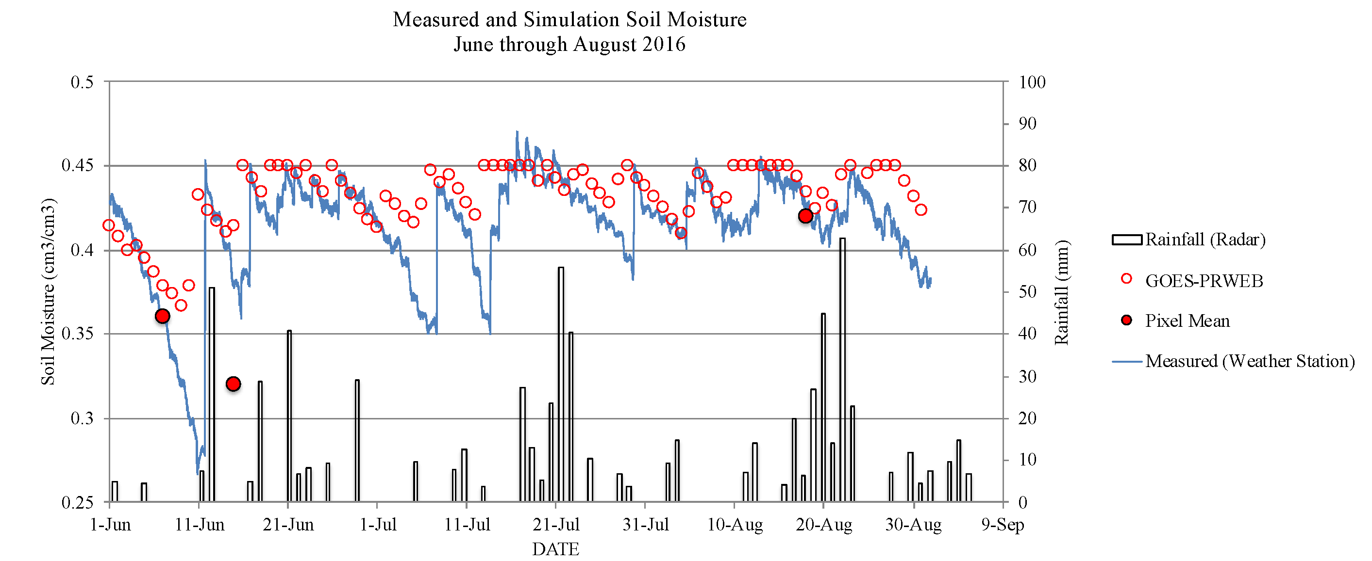
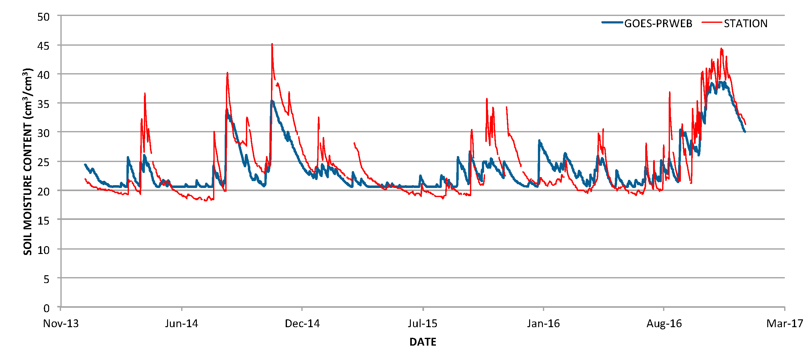
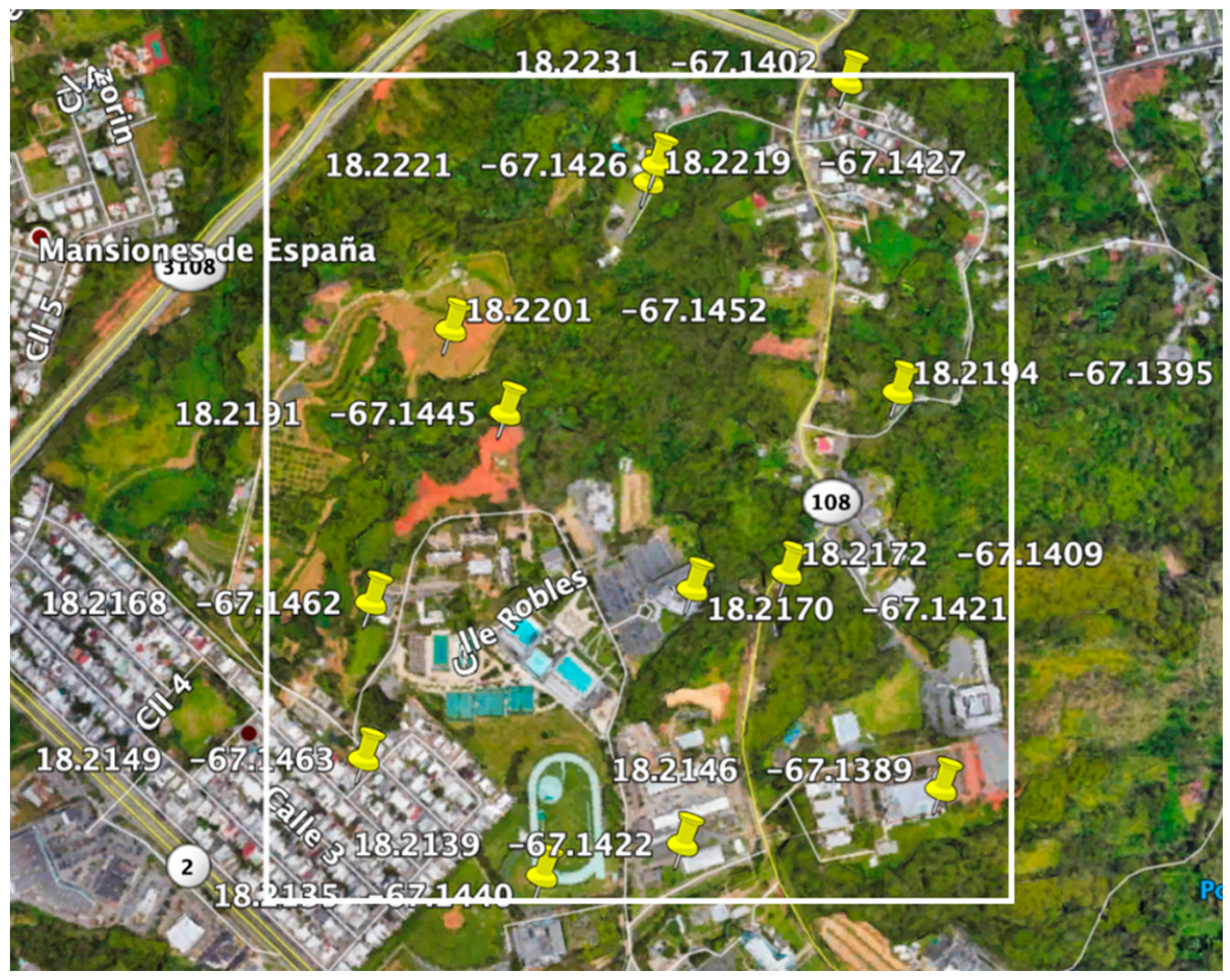
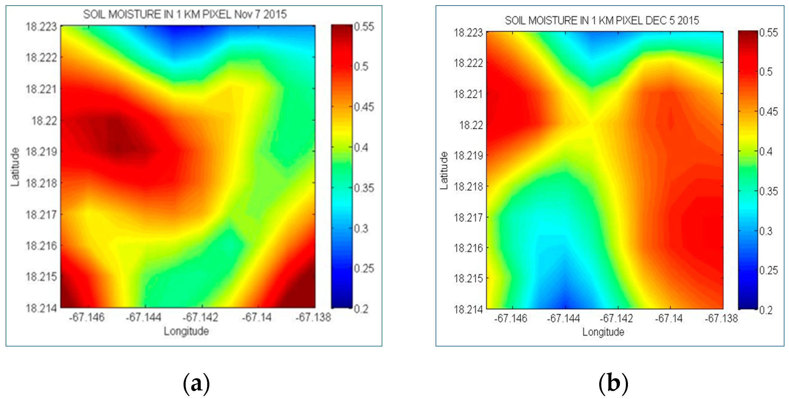
2.7. Evaluation of Soil Moisture Estimates

GOES-PRWEB produces a single value of θ for the 1-km² pixel area. We hypothesized that there was high variability in θ within a 1-km² GOES pixel. Notwithstanding the measured variability, we further hypothesized that GOES-PRWEB could estimate the average measured θ for the 1-km² area. Undisturbed soil samples were taken to measure the water content at various locations within the studied pixel to test these hypotheses. The study area is located on the University of Puerto Rico-Mayaguez (UPRM) campus in western Puerto Rico. Samples were obtained on 1 October, 13 October, 7 November, and 5 December 2015, and 7 June, 27 June, and 18 August 2016.

Sample locations are presented in Figure 1; some areas of the study pixel in the southwest and the northeast fall outside the UPRM campus. The study area was selected because it corresponded with a GOES visible channel pixel. Soil cores were used to collect soil samples within the study pixel for water content analyses. GPS coordinates were obtained, and organic matter was cleared from the area upon arrival. The metal cores were hammered into the soil with a mallet until the top rim of the core was level with the surface, and a shovel was used to carefully extract the soil-filled core from the ground. Soil samples were quickly removed from the soil core, inserted into a labeled plastic bag, and weighed in the field to record the exact weight of the wet or damp soil. Later, the soil samples were dried with a microwave oven for approximately 20 min, and the dry weight was recorded.

The undisturbed θ was estimated from the following equation: θ_v [cm³ cm⁻³] = (WW_nudist − DW_undist)/(Vol ρ_H2O), where WW_undist is undisturbed soil wet weight (gm), DW_undist is undisturbed soil dry weight (gm), Vol is the volume of the sample core (cm³), and ρ_H2O is the density of water (1 gm cm^–3). Average θ estimates from weather station sensors (Watchdog ET900, Spectrum Technology, Inc., Aurora, IL, USA) located at the Agricultural Engineering Building on the UPRM Campus were also compared with the gravimetric and GOES-PRWEB estimates. The soil moisture sensors were installed at 0.3 m and 0.6 m depths.

Another soil moisture comparison study was conducted over three years at the UPR Agricultural Experimental Station near Juana Díaz, Puerto Rico. The 1-km² GOES-PRWEB pixel was assigned a root depth of 1 m, while the station data were based on a weighted average of θ sensors (Time Domain Reflectometry) at depths of 0.0508 m, 0.1016 m, 0.2032 m, 0.508 m, and 1.016 m.

2.8. Island-Scale Comparisons

Two island-scale validation studies were conducted:

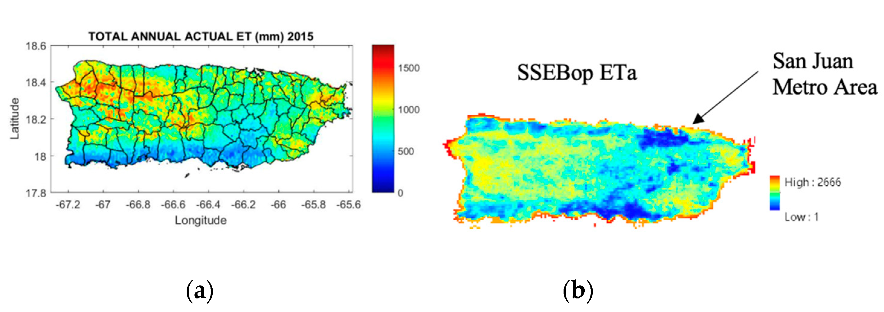
• Annual ET_a from GOES-PRWEB and the SSEBop model were compared for 2009–2020;
• Annual values of the water balance components from GOES-PRWEB and the USGS ([62]) were compared for 2009–2020.

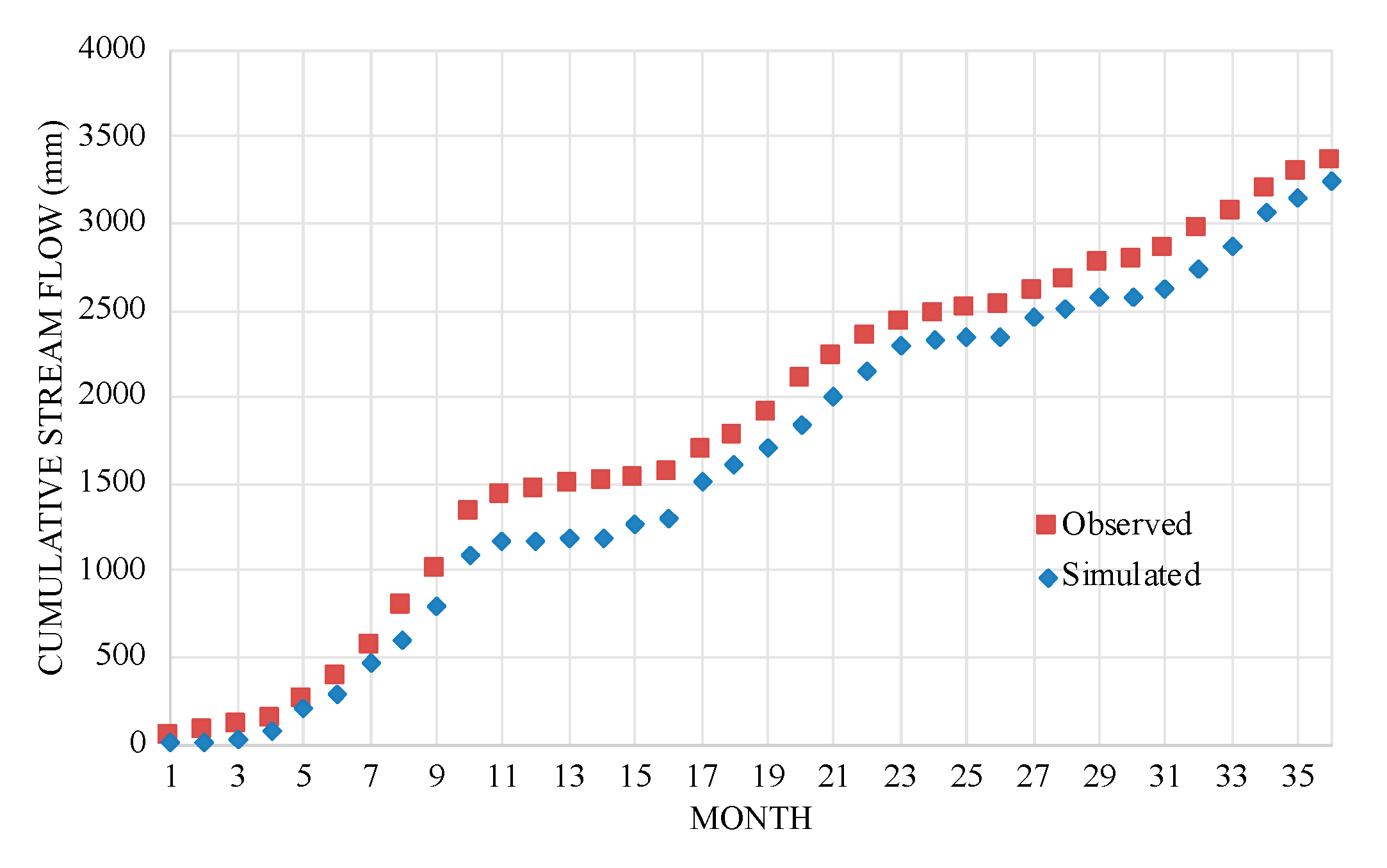
2.9. Basin-Scale Comparisons

Two basin-scale validation studies were conducted:

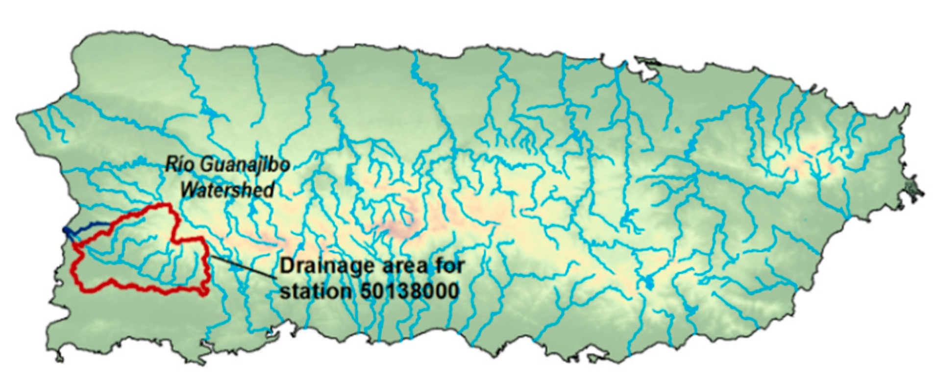
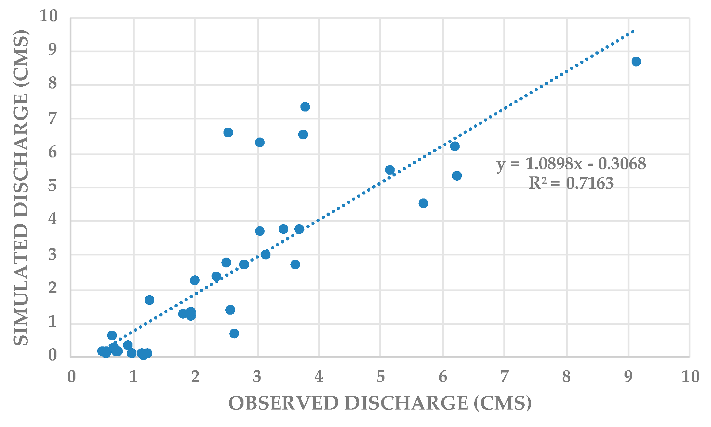
• Comparisons of cumulative monthly streamflow were made for GOES-PRWEB and the US Geological Survey (USGS) stream gage located at the outlet of the Guanajibo watershed in southwest Puerto Rico for the years 2010, 2011, and 2012. Total streamflow was assumed to be the combined flow from surface runoff and deep percolation, where the latter contributes to the stream base flow. Since the model does not explicitly account for groundwater storage, this may be a source of error during short periods. However, over more extended periods, such as a year and during hydrologically normal years, the change in storage was small.
• GOES-PRWEB and USGS-based annual ETa estimates were compared for the Guanajibo watershed for 2009–2020. The USGS-based ETa was estimated as P − (RO + DP), where (RO + DP) is considered to be equal to the total measured streamflow.

2.10. Pixel Scale Comparison

A pixel-scale validation study was conducted:

A comparison of monthly ET_a at three locations in Puerto Rico from January 2010 to December 2012 was conducted.

2.11. Water Balance Error Analyses

To verify the numerical correctness of the model, island-scale and pixel-scale water balance error analyses are presented.

3. Results

In this section we present results to support the validation of the model.

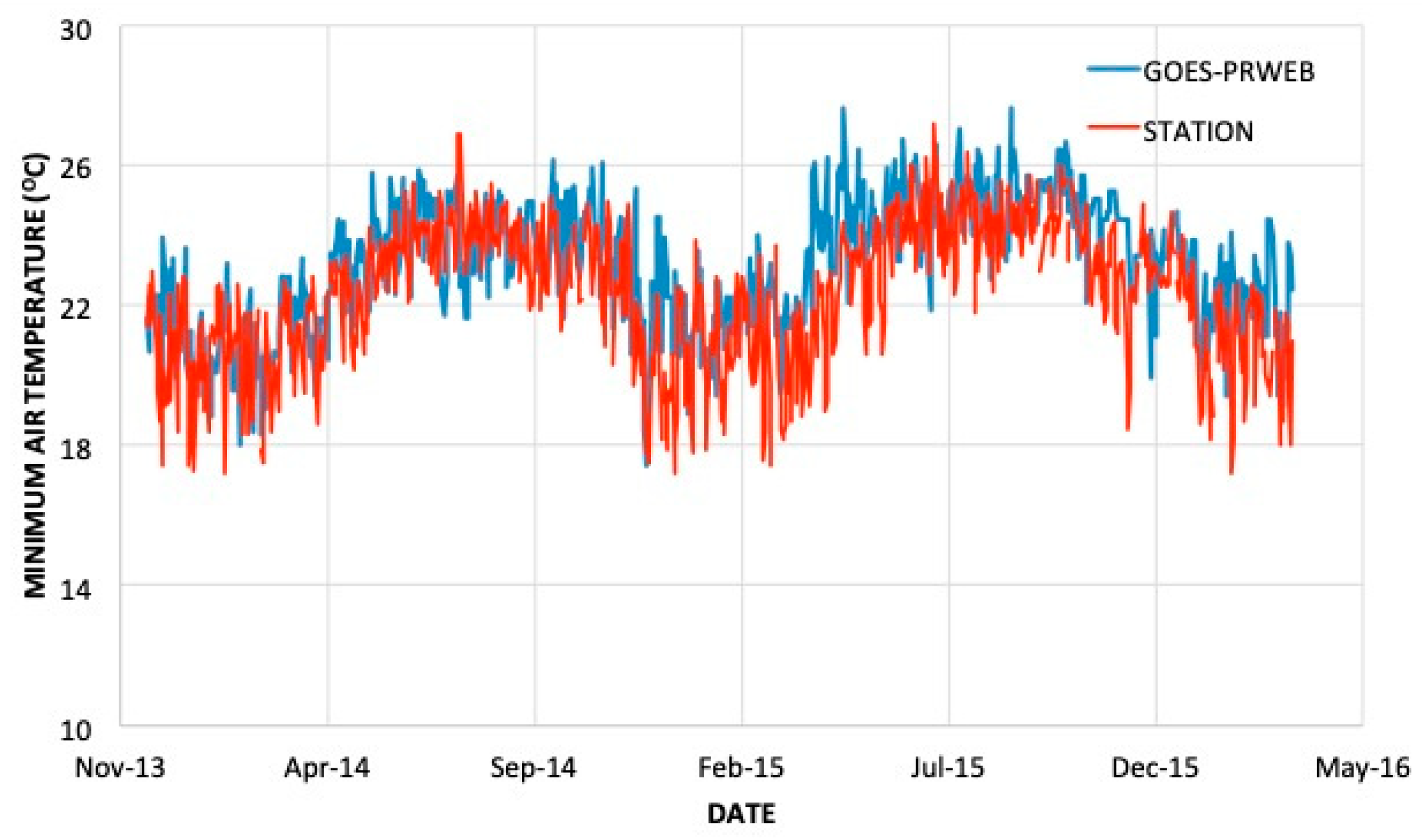
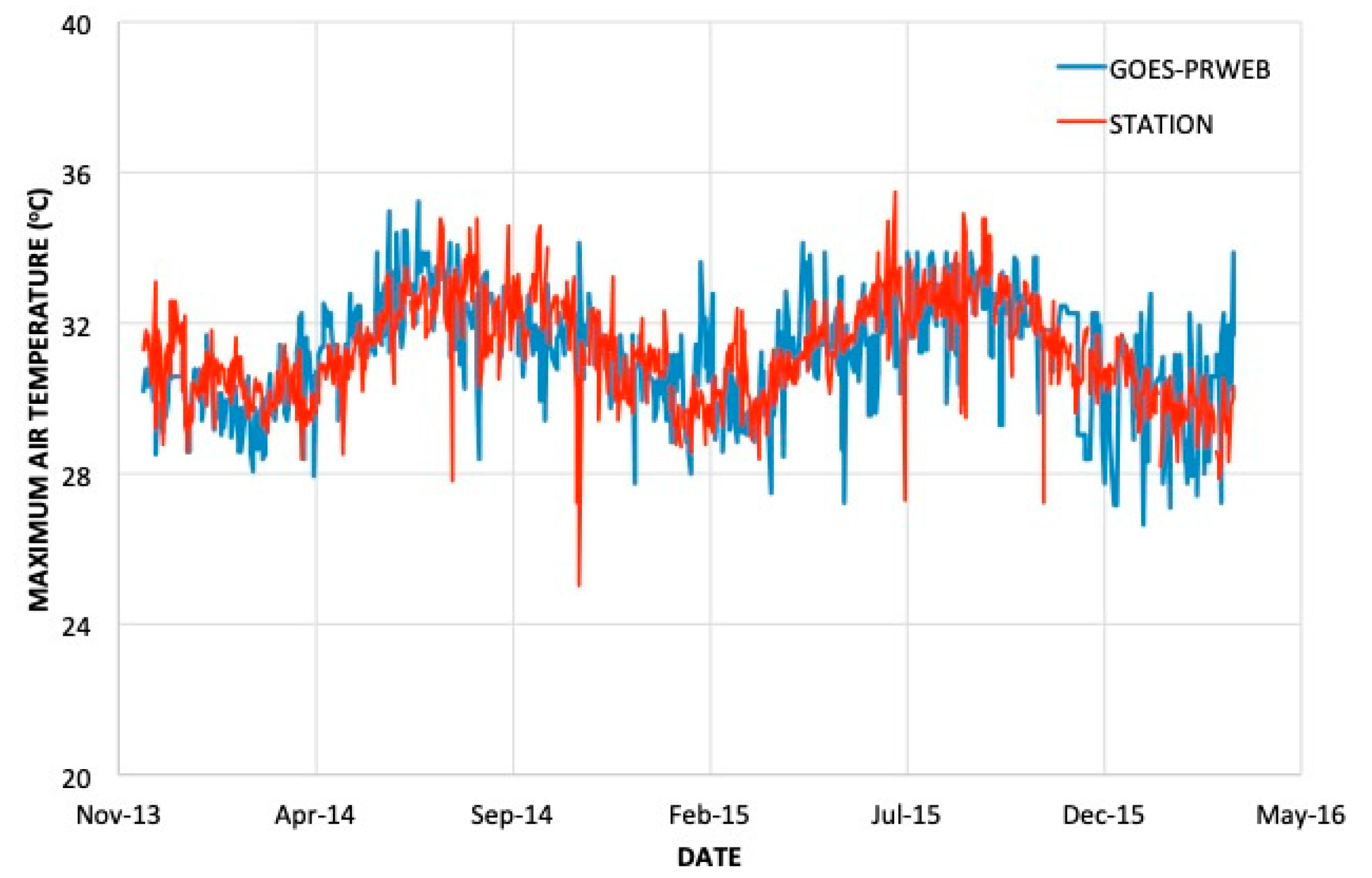
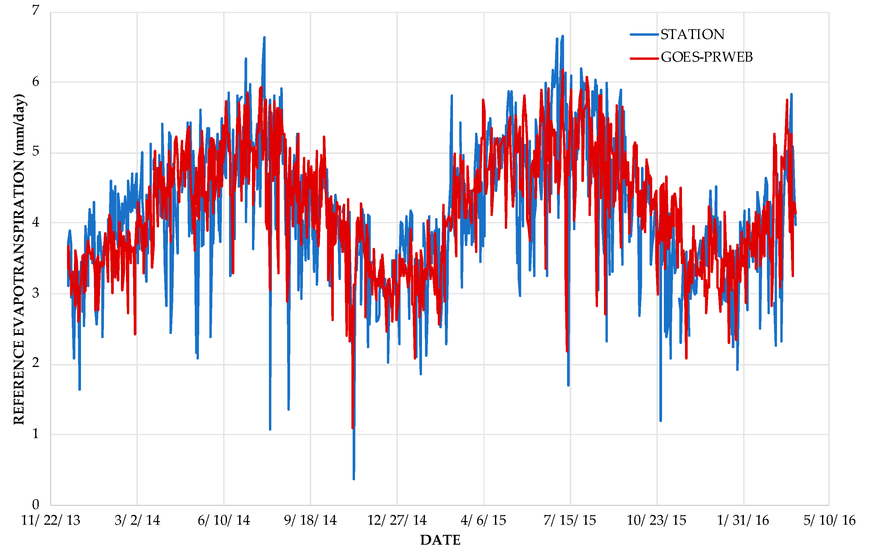
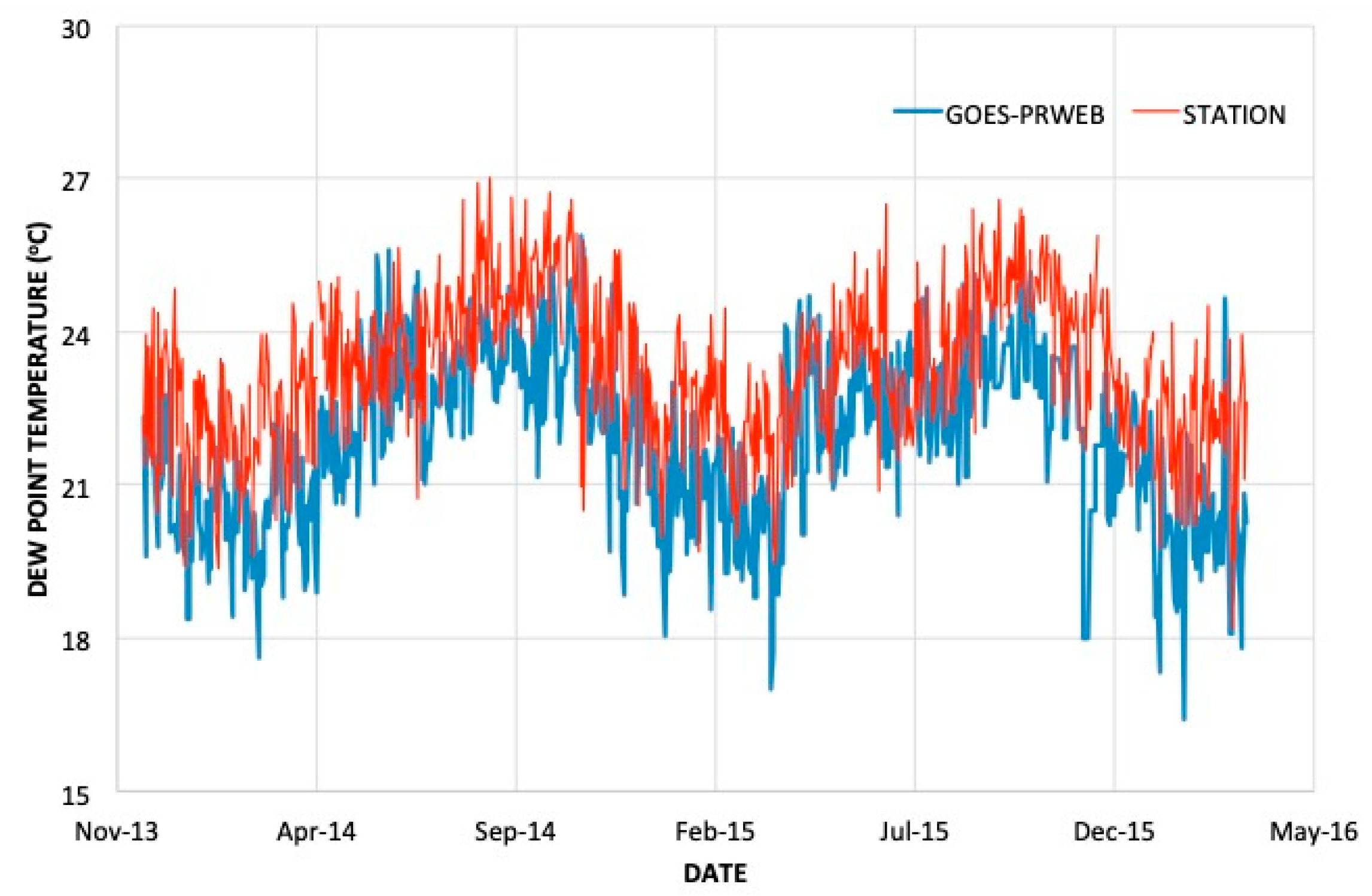
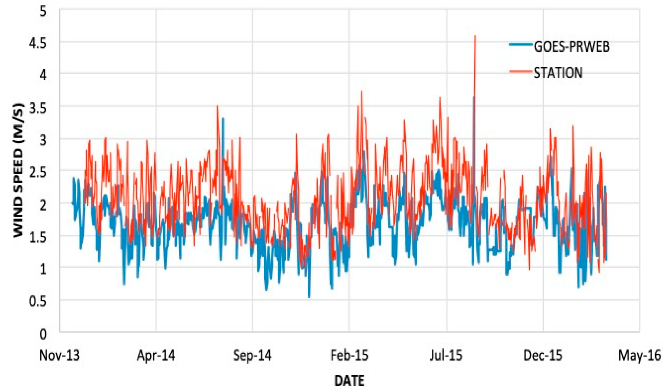
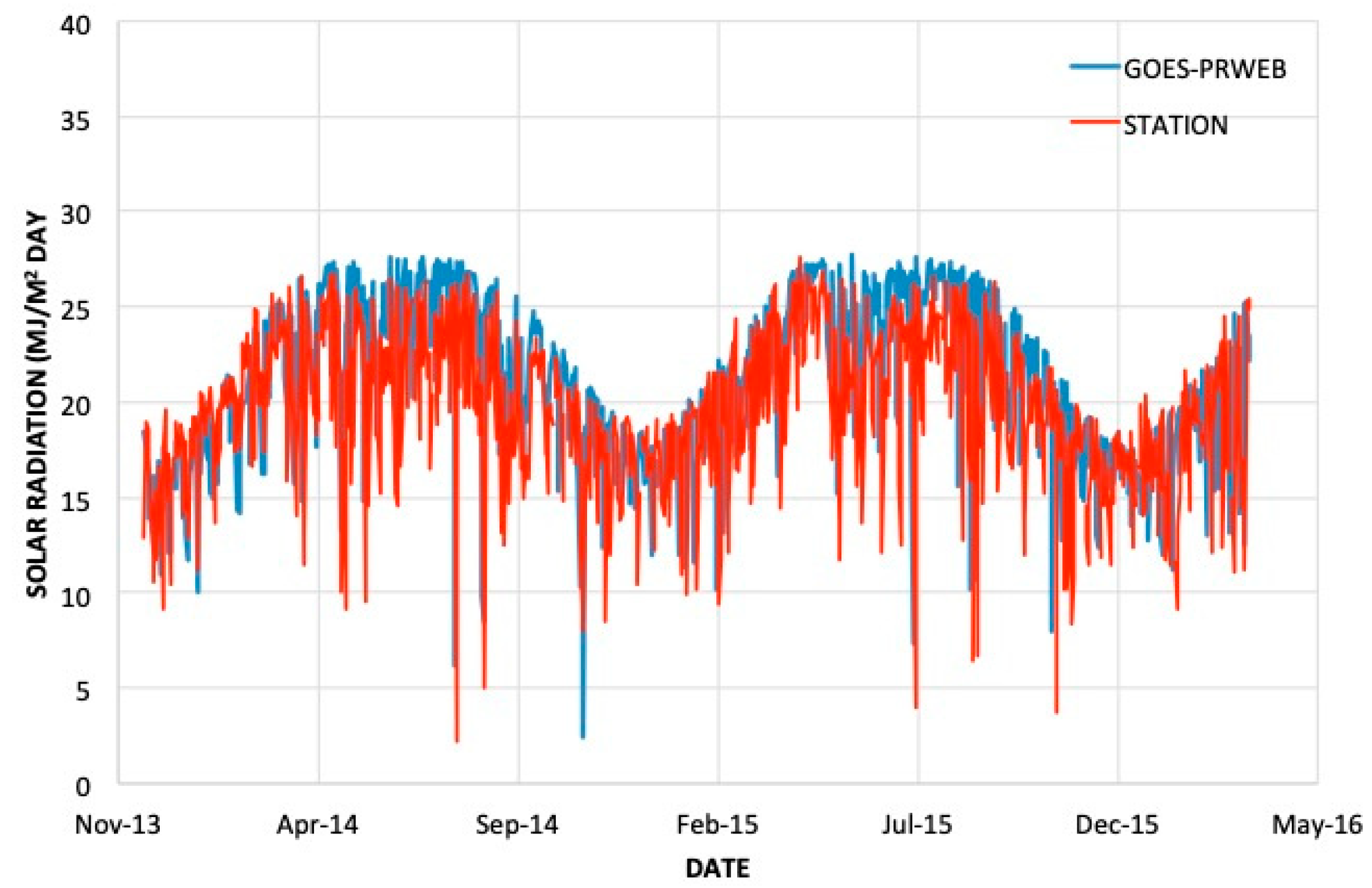
3.1. Evaluation of ETo and Other Weather Parameters

Figure 2 shows a time series of the estimated ET_o at the UPR Agricultural Experimental Station near Juan Diaz, Puerto Rico (latitude 18.033 degrees, longitude −66.533 degrees) from January 2014 to April 2016. The GOES-PRWEB-derived ET_o is in good agreement with the ET_o from the NRCS SCAN weather station. To better understand the model-estimated ET_o, it is necessary to consider the model’s climate input data. For the interested reader, graphs of the associated T_min, T_max, T_d, u₂ and R_s are presented in Appendix A. The temperature and wind speed data used as input to GOES-PRWEB were derived from gridded model data from NOAA’s NDFD website, and R_s was derived from the GDM radiative transfer method using GOES-13 satellite data. The T_min (Figure A1) was slightly overestimated relative to the weather station data. On average, T_max (Figure A2) was consistent with the station data; however, gridded data was characterized with more significant variability during specific periods. T_d (Figure A3) was under-estimated relative to the weather station data. u₂ data (Figure A4) was under-estimated relative to the weather station data, and R_s data (Figure A5) was reasonably accurate relative to the weather station.

Table 1. Statistical results of ET_o and weather parameters associated with data presented in Figure 2 and Figure A1, Figure A2, Figure A3, Figure A4 and Figure A5.

	GOES-PRWEB Average	Station Average	Average % Error	Significant Difference
ETo (mm day−1)	4.22	4.18	0.96	No
Tmin (°C)	23.16	22.37	3.51	Yes
Tmax (°C)	31.15	31.24	−0.14	No
Td (°C)	21.24	23.27	−8.72	Yes
u2 (m s−1)	1.69	2.08	−18.85	Yes
Rs (MJ m−2 day−1)	18.94	21.03	−9.93	No

summarizes the statistics related to the comparison data presented in Figure 2 and Figure A1, Figure A2, Figure A3, Figure A4 and Figure A5. The average error was calculated as follows: 100 [(GOES-PRWEB Average − Station Average)/Station Average]. The average error in the ET_o was 0.96%, and the weather variable with the most significant average error was u₂ with 18.94%. Statistical significance was determined based on forty random samples from each of the variables’ time series. Observed and modeled ET_o, T_max, and R_s were not significantly different at the 0.05 level. Observed and modeled T_min, T_d, and u₂ were significantly different.

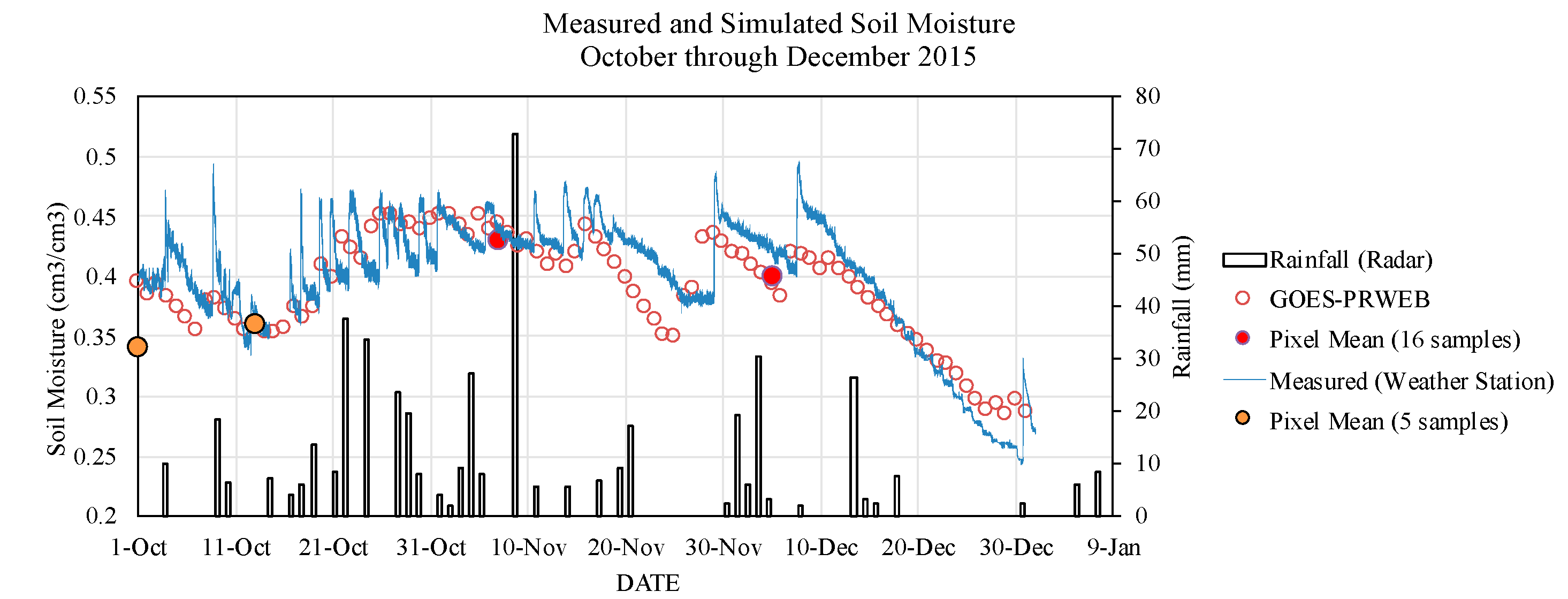
3.2. Evaluation of Soil Moisture Estimation

Figure 3 shows the distribution of measured soil water content on 7 November and 5 December 2015, respectively, within a 1-km² GOES pixel on the UPRM campus. The results confirmed that there was indeed high variability in the soil water content within the studied pixel, as hypothesized. Figure 4 and Figure 5 compare θ from GOES-PRWEB (daily values), undisturbed soil samples (pixel average), and the average of two weather station sensors located at the Agricultural Engineering Building on the UPRM campus. Pixel average water content values were obtained during October, November, December 2015, and June and August 2016. Five samples were obtained during October 2015, and thirteen samples were obtained during all other months. The θ values from the pixel average agreed with the estimates of θ from GOES-PRWEB for six of the seven sampling events. The period corresponding with Figure 4 was rainy, and the soil was relatively wet. This is observable because the GOES-PRWEB θ reached the soil field capacity of 0.45 on numerous occasions. During one sampling event on 18 June 2016 (Figure 5), the measured pixel average θ was significantly lower than GOES-PRWEB (difference approximately 0.08). During the summer of 2016, θ from the weather station sensors frequently dropped below GOES-PRWEB. However, this discrepancy is not of great concern, considering that the weather station water content represents only a single point within the 1-km² pixel area. It should be noted that the undisturbed core samples were taken from the top 0.127 m, the two weather stations sensors were installed at 0.3 and 0.6 m, and the GOES-PRWEB assigned root depth was from 0 to 0.87 m. These differences in the three methods’ soil control volumes may have contributed to the observed discrepancies.

As another check on the ability of the model to simulate θ, Figure 6 shows a comparison of the estimated and measured (depth-averaged) daily volumetric moisture content at the UPR Agricultural Experiment station near Juana Diaz, Puerto Rico, from 1 January 2014 to 31 December 2016. Soil moisture sensors were located at the following depths: 0.0508 m, 0.1016 m, 0.2032 m, 0.508 m, and 1.016 m. The average GOES-PRWEB θ, average station θ, average percent error, and R² for the data presented in Figure 6 were 23.9%, 24.39%, −2.13%, and 0.75, respectively. A Student t-test was performed on 40 randomly selected soil moisture pairs from the 3-year dataset, indicating no significant difference at the 0.05 level between the mean observed and simulated values (t(39) = 0.42104, p = 0.674854).

3.3. Basin-Scale Streamflow Comparison

The cumulative simulated and observed stream flows from the Guanajibo watershed (USGS gage station at Hormigueros, No. 50138000, catchment area 310.9 km²) were compared. Figure 7 shows the location of the gaged catchment area (red) and the entire watershed (black).

Figure 8 shows a comparison of the cumulative GOES-PRWEB (simulated) and observed stream flows for the Guanajibo catchment area for 36 months (2010, 2011, and 2012). The streamflow results are presented in millimeters, obtained by dividing the monthly flow volume by the applicable catchment area (310.5 km²).

The mean error in the monthly flow for the Guanajibo River for the 36-month comparison is −2.6%, indicating that simulated streamflow was, in general, less than the observed. In general, the simulated vs. observed streamflow was in good agreement. Applying a two-tailed Student t-test, no significant difference was found between the observed and simulated mean monthly streamflow at the 0.05 level (t(35) = 0.17268, p = 0.863403). Figure 9 shows the simulated versus the observed stream discharge and Figure 10 shows the monthly simulated versus observed stream discharge. The results show generally good agreement; however, there were four months (months 5, 17, 33 and 34) when the model significantly overestimated the stream discharge. It is also noted that the model tended to underestimate stream flow during periods of low flow. The calculated coefficient of determination for the monthly analysis was r² = 0.7136.

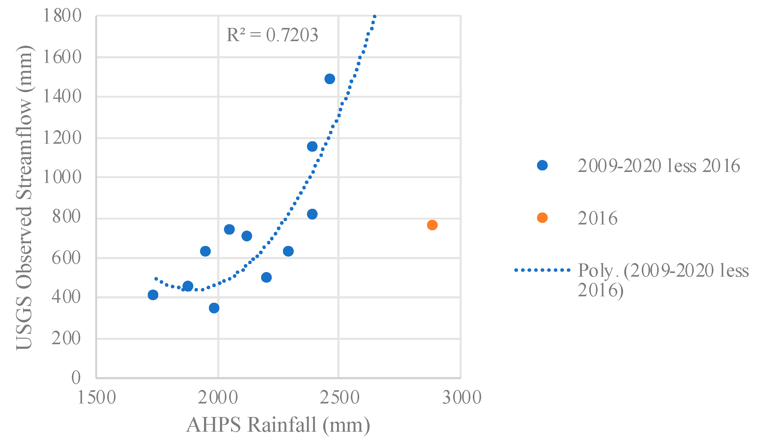
3.4. Basin-Scale Actual Evapotranspiration Comparison

Independent flux tower data are not available for the period of the study in Puerto Rico. As an alternative, we compared the basin-scale annual average GOES-PRWEB ET_a with a USGS-based ET_a. In the latter case, ET_a = P − (RO + DP), where RO + DP is the total streamflow derived from the USGS stream gage on the Guanajibo River near Hormigueros, Puerto Rico (Figure 7), and P data were obtained from NOAA’s AHPS website, which is bias-corrected radar rainfall.

Table 2. Comparison of the Guanajibo watershed annual ET_a derived from AHPS rainfall and USGS Streamflow data * with GOES-PRWEB ET_a for 2009–2020.

Year	AHPS Rainfall (mm)	USGS Stream-Flow (mm)	USGS ETa (mm)	GOES-PRWEB ETa (mm)	Error (%)
2009	2130	703	1335	1317	−1.35
2010	2398	1144	1151	1311	13.90
2011	2396	808	1485	1276	−14.07
2012	2301	621	1540	1337	−13.18
2013	1890	445	1357	1259	−7.22
2014	1997	343	1577	1278	−18.96
2015	1746	400	1271	1226	−3.54
2016	2886	757	2129	1304	−38.75
2017	2473	1483	990	1060	7.07
2018	2205	487.9	1717	1369	−20.27
2019	1961	621	1340	1277	−4.70
2020	2054	732	1322	1350	2.12
		Average	1371	1278	−6.80

* USGS ETa = AHPS Rainfall − USGS Stream flow.

shows the annual basin analyses for 2009–2020 (2016 was removed; see explanation below). The minimum, maximum, and mean errors in the model ET_a for the 12 years were −1.35% (2009), −18.96% (2014), and −6.8%, respectively. Error is equal to 100 (GOES-PRWEB ET_a − USGS ET_a)/USGS ET_a. When applying a two-tailed Student t-test, no significant difference at the 0.05 level was found between the observed and simulated mean annual ET_a (t(11) = 1.40728, p = 0.174695).

The 2016 ET_a estimate from AHPS rainfall and USGS streamflow data was abnormally high and therefore was discarded from the analysis. The cause of the high estimated ET_a was the anomalously low value of streamflow, despite that year having the highest recorded rainfall for all the years considered. Figure 11 shows that the 2016 streamflow was an outlier, hence justifying its removal from the dataset.

3.5. Actual Evapotranspiration Evaluation

3.5.1. Island-Wide ETa Evaluation

Annual actual evapotranspiration from the Simplified Surface Energy Balance (SSEBop) model [38] was compared with GOES-PRWEB for 2009–2020 (

Table 3. Comparison of SSEBop and GOES-PRWEB annual ETa for 2009–2020.

Year	AHPS Rainfall (mm)	SSEBop ETa (mm)	GOES-PRWEB ETa (mm)	Error (%)
2009	2130	1204	1223	1.58
2010	2398	1244	1250	0.48
2011	2396	1232	1247	1.22
2012	2301	1229	1250	1.71
2013	1890	1193	1190	−0.25
2014	1997	1137	1182	3.96
2015	1746	1116	999	−10.48
2017	2473	1178	1201	1.95
2018	2205	1155	1045	−9.52
2019	1961	1182	1167	−1.27
2020	2054	1109	1130	1.89
Average	2141	1180	1171	−0.73

). SSEBop, a product of the Famine Early Warning Systems Network (FEWS NET), estimates ET_a based on a fractional weighting of ET_o using Moderate Resolution Imaging Spectrometer (MODIS) thermal imagery, obtained every eight days. The original formulation of the SSEBop model is based on the SEBAL ([63]) and METRIC ([35]) algorithms.

In most years, the percent difference (error) between the two models was small. The largest errors occurred in 2015 and 2018. Puerto Rico experienced a devastating drought during 2015 (AHPS rainfall 1746 mm). On the other hand, 2018 was a relatively wet year (AHPS rainfall 2205 mm). The overall average error was −0.73 percent, and there was no significant difference at the 0.05 level between the mean SSEBop and GOES-PRWEB annual ET_a (Student-t statistics: t(11) = 0.30016, p = 0.767154).

Figure 12 shows the GOES-PRWEB and SSEBop annual ETa spatial distribution for 2015. SSEBop produced lower values of ETa in the San Juan Metropolitan area. It has been observed that the SSEBop model produces low values of ET_a in coastal urban areas (personal communication, Nick Sepulveda, USGS). On the other hand, GOES-PRWEB may be overestimating ETa in the Metro area. Note that the SSEBop model produced very high values all around the coast (2666 mm) in the pixels adjacent to the ocean. Presumably, SSEBop produces high values of ETa in these pixels because the MODIS thermal image combines ocean and land within the same pixels. Consequently, the estimate is approaching the potential evapotranspiration. GOES-PRWEB does not suffer from this problem because the land surface temperature estimation is based only on the energy balance of the land properties. For the comparison in this study (Table 3), the high SSEBop ETa values along the coasts were removed.

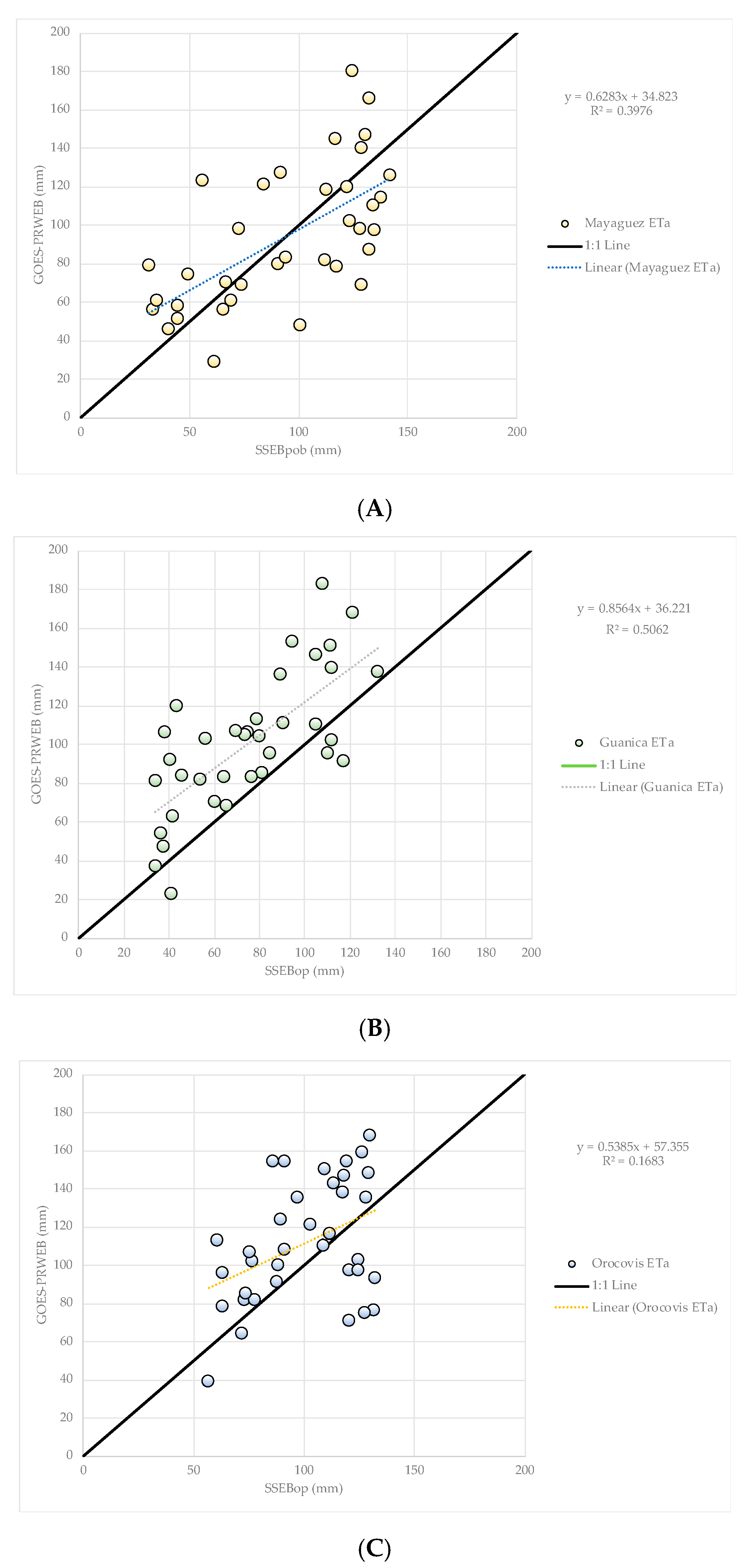
3.5.2. ET_a Evaluation at Three Locations

Here, we compare the GOES-PRWEB and SSEBop ET_a at three locations in Puerto Rico: Mayagüez, Guánica, and Orocovis. The conditions at each pixel are summarized in

Table 4. Conditions at the three ET_a comparison sites.

Site	Lon	Lat	Elevation (m)	Land Cover	Climate
Mayagüez	18.22	−67.146	36	Urban and Built up	Humid
Guánica	17.95	−66.940	30	Woodlands	Semi Arid
Orocovis	18.20	−66.470	985	Deciduous Forest	Humid

. Figure 13A–C show the GOES-PRWEB versus SSEBop ET_a for Mayagüez, Guánica and Orocovis, respectively. It should be noted that the 1-km resolution SSEBop ET_a product is not calibrated for PR. Consequently, we will use the term “Deviations” instead of errors. Deviations were estimated as 100(GOES-PRWEB ET_a − SSEBop ET_a)/SSEBop ET_a. The mean monthly deviations were 0.07%, 25.14%, and 9.8% for Mayagüez, Guánica, and Orocovis, respectively.

Paired comparisons of the mean GOES-PRWEB and mean SSEBop for the three locations, using the Student’s t-test, were performed. While there was no significant difference at the 0.05 significance level between the Mayaguez means (t(35) = −0.00731, p = 0.99419) and Orocovis means (t(35) = −1.6481, p = 0.103813), there was a significant difference between the means for Guánica (t(35) = −3.29467, p = 0.000774). Because the SSEBop ET_a product is not calibrated for PR, it is not possible to determine which model is more accurate. Nevertheless, there is a degree of correlation between the two models (Figure 13A–C), which provides credibility to the GOES-PRWEB results for the relatively diverse environmental conditions evaluated (i.e., elevation, land cover and climate).

3.6. Island-Wide Water Balance Component Comparison

The USGS published estimates of the average water balance components for Puerto Rico ([62]) as follows: P 1829 mm, ET_a 1168 mm, streamflow (RO + base flow [=DP]) 635 mm, groundwater discharge from coastal aquifers to wetlands, estuaries and seabed 25 mm, groundwater withdrawals from coastal aquifers 25 mm, and soil moisture and groundwater storage 25 mm. In terms of rainfall percentages: ET 63.9%, total streamflow (RO + DP) 34.7%, groundwater discharge from coastal aquifers to wetlands, estuaries, and seabed 1.3%, groundwater withdrawals from coastal aquifers 1.3%, and soil moisture and groundwater storage 1.3%.

GOES-PRWEB-estimated water balance components for Puerto Rico from 2009–2020 are presented in

Table 5. Water balance components for Puerto Rico, 2009–2020.

Year	Rainfall (mm)	ETa (mm)	RO + DP * (mm)	Runoff (mm)	Deep Percolation (mm)	Balance: Rainfall − ETa − (RO + DP) (mm)
GOES-PRWEB
2009	1631	1223	446	360	86	−38
2010	2204	1250	967	741	227	−14
2011	2246	1247	1020	790	230	−21
2012	1837	1250	614	498	116	−27
2013	1830	1190	637	483	154	3
2014	1611	1182	500	417	83	−71
2015	1415	999	407	335	73	8
2016	2140	1201	925	677	248	14
2017	2653	1045	1644	1122	523	−37
2018	1729	1167	622	447	181	−66
2019	1584	1130	407	343	64	47
2020	1785	1234	551	427	124	0
Standard Deviation	353.9	81.5	359.5	236.1	127.1	33.9
Average	1888.8	1176.5	728.3	553.3	175.8	−16.8
Percent of Rainfall	100.0%	62.3%	38.6%	29.3%	9.3%	−0.9%
USGS [62]
Average	1829.0	1168.0	635.0			27.0
Percent of Rainfall	100.0%	63.9%	34.7%			1.5%

* DP for the USGS includes aquifer recharge, groundwater discharge from coastal aquifers to wetlands, estuaries, seabed, and groundwater withdrawals from coastal aquifers.

and compared with the USGS estimates (included in the table). The table shows the water balance components in depths of water in mm and as percentages of rainfall. Average GOES-PRWEB P was 1888.8 mm, ET was 1176.5 mm, and total streamflow (RO + DP) was 728.3 mm.

The GOES-PRWEB and USGS island-wide average ET_a, as a percentage of rainfall, were 62.3% and 63.9%, respectively; and the RO + DP were 38.6% and 34.7%, respectively. The island-wide average ET_a and RO + DP results from GOES-PRWEB and the USGS are in good agreement.

3.7. Water Balance Error Analyses

3.7.1. Pixel-Scale Water Balance Error Analyses

In this section, the water balance errors are analyzed at the pixel-scale at Mayagüez, Guánica and Orocovis (Table 4). Ideally, P_i − ET_ai − RO_i − DP_i + (SM_i−1 − SM_i) should equal zero; however, due to numerical errors in the algorithm, water balance errors can occur. Numerical errors may include rounding errors or lack of convergence by the recursive root function employed in the methodology. The subscripts i and i − 1, represent the current and previous time steps.

Table 6. Annual overall mean, minimum and maximum water balance errors for Mayaguez, Guánica and Orocovis for 2009–2020. All values are in millimeters.

	Mean Error (mm)	Minimum Error (mm)	Maximum Error (mm)
Mayagüez
Mean (2009–2020)	0.01	−1.5	20.78
Std. Dev.	0.07	0.93	8.33
Guánica
Mean (2009–2020)	0.05	−1.38	21.6
Std. Dev.	0.04	0.98	8.49
Orocovis
Mean (2009–2020)	0.04	−0.73	16.49
Std. Dev.	0.03	1.28	8.04

presents the average overall mean, minimum, and maximum balance errors for the three locations. The sample size was n = 12 (2009–2020). All values are in millimeters. The overall mean annual errors for the three locations are all less than 0.05 mm and can be considered negligible. The largest overall mean annual negative error was −1.38 mm, while the largest overall mean annual positive error was 21.6 mm. The results in Table 6 are based on mean annual estimated errors presented in Appendix B (

Table A1. Daily mean, standard deviation, minimum and maximum water balance e errors at Mayaguez, Puerto Rico. Table also includes annual values. All values are in millimeters.

Year	Daily Mean Error (mm)	Std Dev. (mm)	Minimum Error (mm)	Maximum Error (mm)
2009	−0.07	2.13	−3.06	14.91
2010	−0.06	2.00	−2.22	13.20
2011	0.02	2.26	−2.21	10.37
2012	0.05	2.45	−2.03	16.88
2013	0.02	2.11	−2.25	8.03
2014	−0.01	2.42	−2.01	13.83
2015	0.01	2.42	−1.96	13.87
2016	0.01	2.28	−2.40	11.31
2017	−0.02	2.54	−2.25	13.02
2018	−0.05	2.06	−1.85	8.18
2019	0.06	2.23	−1.84	14.24
2020	−0.02	2.19	−2.04	12.44
Annual Mean Error	0.00	2.26	−2.18	12.52
Std. Dev.	0.04	0.17	0.33	2.65

,

Table A2. Daily mean, standard deviation, minimum and maximum water balance e errors at Guanica, Puerto Rico. Table also includes annual values. Table also includes annual values. All values are in millimeters.

Year	Daily Mean Error (mm)	Std Dev. (mm)	Minimum Error (mm)	Maximum Error (mm)
2009	0.01	3.42	−1.87	33.16
2010	0.04	3.19	−2.54	22.69
2011	0.01	3.38	−2.39	24.11
2012	−0.02	3.29	−2.24	22.20
2013	0.07	3.00	−1.97	26.69
2014	−0.02	3.22	−2.31	38.00
2015	−0.10	1.61	−1.57	11.11
2016	0.10	3.02	−1.95	22.45
2017	−0.04	2.62	−2.17	23.58
2018	−0.10	1.68	−1.41	13.87
2019	0.10	2.32	−1.79	27.55
2020	0.04	3.12	−1.95	27.91
Annual Mean Error	0.01	2.82	−2.01	24.44
Std. Dev.	0.07	0.63	0.33	7.32

and

Table A3. Daily mean, standard deviation, minimum and maximum water balance e errors at Orocovis, Puerto Rico. Table also includes annual values. Table also includes annual values. All values are in millimeters.

Year	Daily Mean Error (mm)	Std Dev. (mm)	Minimum Error (mm)	Maximum Error (mm)
2009	−0.04	1.86	−2.93	11.82
2010	−0.02	1.88	−2.47	17.29
2011	−0.01	1.72	−1.65	12.44
2012	0.03	1.95	−1.63	15.47
2013	0.02	1.99	−1.94	13.78
2014	−0.02	2.42	−2.20	25.28
2015	−0.02	1.86	−1.79	10.66
2016	0.04	1.81	−2.72	9.64
2017	−0.08	1.96	−2.39	13.80
2018	−0.01	1.68	−2.04	9.41
2019	0.08	2.10	−2.67	13.18
2020	−0.02	2.21	−2.39	18.15
Annual Mean Error	0.00	1.95	−2.23	14.24
Std. Dev.	0.04	0.21	0.43	4.43

).

3.7.2. Island-Wide Water Balance Error Analysis

Table 7. GOES-PRWEB water balance (Rainfall − ET_a − RO + DP-change in soil moisture).

1	2	3	4	5	6
Year	θJan 1	θDec 31	θJan 1 − θDec 31	Rainfall − ETa − RO+DP (% of Rainfall)	Water Balance Error (col 5 − col 4, % of Rainfall)
2009	30.9%	30.0%	−0.9%	−2.3%	−1.4%
2010	29.9%	28.5%	−1.4%	−0.6%	0.8%
2011	28.7%	27.9%	−0.7%	−0.9%	0.2%
2012	29.9%	30.9%	1.0%	−1.5%	−2.5%
2013	30.7%	30.2%	−0.4%	0.2%	0.6%
2014	30.3%	26.7%	−3.5%	−4.4%	0.9%
2015	26.3%	27.4%	1.1%	0.6%	−0.5%
2016	27.2%	31.4%	4.2%	0.7%	−3.5%
2017	32.3%	28.8%	−3.5%	−1.4%	2.1%
2018	28.8%	26.3%	−2.5%	−3.8%	−1.3%
2019	26.2%	29.8%	3.6%	3.0%	−0.6%
2020	29.9%	29.8%	−0.1%	0.0%	0.1%
Average	29.2%	29.0%	−0.2%	−0.9%	−0.7%

compares the model water balance error as a percent of rainfall from 2009–2020. Annual change in soil moisture is the difference between the soil moisture on the first and last day of the year. If the model has no water balance error, then the value in column 6 would be zero. The average water balance error is −0.7%. The annual water balance errors are sufficiently small, indicating that the island-wide water balance is acceptable.

4. Discussion and Conclusions

4.1. Model Applications

The model has been used for various practical applications. For example, [64] reported a web-based GOES-PRWEB method for scheduling irrigation in PR, USVI, Hispaniola, Jamaica, and Cuba. The USGS used GOES-PRWEB to estimate water use by agricultural crops as part of a water withdrawal and use study in Puerto Rico ([65]). The Scientific Drought Committee of Puerto Rico uses data from the model in their weekly reports [66]. NOAA’s National Weather Service (NWS) in San Juan links the near-real-time soil moisture and soil saturation products on their Climate and Drought Information page (https://www.weather.gov/sju/dss_climo, accessed on 15 May 2021). The U.S. Forest Service and the National Integrated Drought Information System (NISDIS) uses soil moisture, soil saturation, and rainfall deficit information from the model for their bi-monthly reports in Puerto Rico and the USVI. Soil saturation from the model was recently used in a Hurricane María flood modeling study in western Puerto Rico ([67]).

4.2. Discussion of Selected Validation Results

Figure 3 shows considerable variability in θ within the 1-km × 1-km study pixel. This finding illustrates the importance of obtaining a multiple soil samples within a study pixel when attempting to validate the soil water content derived using a satellite method. A validation study in which only a single value of soil moisture is used may be insufficient. The need for a greater number of samples increases with coarser resolution soil moisture remote sensing products, such as the Advanced Microwave Scanning Radiometer 2 (AMSR2) with a 25 km spatial resolution ([68]) and the soil moisture active passive (SMAP) mission with a 9 km spatial resolution ([69]).

The modeled and measured θ for the three years, presented in Figure 6, are in reasonably good agreement. However, the model did not produce θ values as high as the station immediately after most rainfall events. A possible explanation for the higher observed θ values is that the mean observed θ is weighted towards the shallow sensors because more sensors are near the surface. Another possible reason is that the observed data reflect moisture contents near the total porosity, whereas the maximum possible moisture content in the model is the field capacity. The above explanation may apply to the slight underestimation of θ by the model during wet periods shown in Figure 4 and Figure 5. It is essential to keep in mind precisely what is being compared in Figure 6, namely the average of five θ sensors installed at a single point with an estimate of θ over an area of 1-km². For this reason, it is not reasonable to expect that the model and measured data would ever be in complete agreement.

Ref. [68] compared the AMSR2 soil moisture product with the NRCS SCAN stations in Puerto Rico. They used two down-scaling techniques to improve the comparisons relative to the raw AMSR2 soil moisture data. The mean error for the Juana Diaz Experimental station was −7.5% for the AMSR2 model vs. −2.13% for GOES-PRWEB in this study (Figure 6). It should be noted that [68] filtered the soil moisture data not using days when the difference between the satellite and station soil moisture values were greater than +/− 0.15. Furthermore, [70] developed an algorithm to estimate soil moisture using a self-organized artificial neural network (ANN) and a stochastic transfer function model for estimating soil moisture at 20 cm depth. Testing the model in Puerto Rico showed that the monthly model had a mean error equal to 2.72%, and the hourly model had mean errors averaging −2.49%. The results from GOES-PRWEB are comparable or better than from the two referenced studies.

For the comparison of monthly stream flow in the Guanajibo Watershed, the mean error for the 36-month period was −2.6%. According to [71], a mean error in stream flow of less than 10% is very good. In addition, [72] calibrated the Vflo model ([73]) for a one-year period (2003) for the same watershed and obtained a mean monthly error 1.8%. Moreover, [74] calibrated a MIKESHE model ([75]), which included surface and groundwater flow for the Añasco, Yagüez and Guanajibo watersheds, and obtained a mean monthly error of 11.7%. Finally, [19] compared stream flow from several models, including GOES-PRWEB, with an improved version of the Water Supply Stress Index (WaSSI) water balance model for the El Yunque National Forest in northeastern Puerto Rico. Unfortunately, the authors incorrectly compared GOES-PRWEB RO with their streamflow instead of RO + DP, which consequently invalidates the comparison.

In this study, a lumped method for the surface runoff for the 1-km² pixel assumes single values of CN and rainfall. In this case, the CN is based on the predominant land use, soil texture, and hydrologic soil group, all of which may have significant spatial variation in the real world. Similarly, in Puerto Rico, rainfall is highly variable spatially and may not be constant within the pixel area. Furthermore, the lead author’s unpublished data collected in Puerto Rico, comparing the AHPS rainfall with rain gage data, indicates that significant rainfall estimation errors can occur. Another possible source of error is the rating curve that the USGS uses to convert the stream depth to stream discharge. Over time, the channel cross-section can change, thus introducing errors into the rating curve. According to the USGS, this was an extensive problem across Puerto Rico, especially after Hurricane María in September 2017 (personal communication, David Hernandez, USGS Hydrologic Data Chief, PR, 16 July 2018).

The DP term in GOES-PRWEB is gross recharge, with a portion potentially going to deep aquifers recharge and a portion, probably the majority, moving laterally through shallow soil or bedrock or to shallow water table aquifers and then discharging to nearby streams. The portion of the DP that flows into the deep aquifers subsequently discharges to the ocean. In the basin-scale stream flow analysis, we assumed that all of DP discharged to the Guanajibo River. This assumption may help explain the overestimation of streamflow for months 5, 17, 33, and 34. On these occasions, it is possible that a larger fraction of the DP went to deep aquifer recharge, and that not all of DP entered the river. It is also noted that the model tended to underestimate streamflow during periods of low flow, which may be because the model does not simulate continuous base flow (i.e., DP); when there is no rainfall, there is no DP or RO. For this reason, the model is not able to estimate daily streamflow.

The basin-scale ET_a analysis yielded a mean annual error for the period 2009–2020 of −6.8%. The analysis compared the annual total ET_a from GOES-PRWEB with an estimate of AHPS rainfall minus the USGS-measured stream flow. This is consistent with a study in the El Yunque National Forest in northeastern Puerto Rico. Using an improved version of the WaSSI model, [19] obtained a relative error of 7% for GOES-PRWEB annual ET_a, relative to their model, for the period 2009–2014. The island-scale annual ET_a analysis for the period 2009–2020 yielded a mean difference between SSEBop and GOES-PRWEB of −0.73%. The pixel-scale ET_a comparison analysis (same period, same models) for the three locations yielded a mean difference of −1.2%. The method described in this paper uses a lumped composite (one-source) flux surface, as opposed to the two source models [76] and [37], which separates the flux surface into soil and vegetated areas (two-source). The two-source method has been shown to provide more accurate results under certain land covers [76]. Future studies should consider comparing the GOES-PRWEB ET_a with the Dis-ALEXI approach. It is also critically important to conduct comparison studies with flux towers in Puerto Rico.

A validation study was also conducted for reference evapotranspiration. ET_o estimates were compared with ET_o derived from a NRCS SCAN weather station at the UPR Agricultural Experiment Station in Juana Diaz, Puerto Rico. The mean error for the 27-month comparison was 0.96%. Furthermore, [42] compared estimated and weighing lysimeter-measured ET_o at Tempe, Arizona for a 26-day period. Estimated ET_o was obtained from the generalized Penman–Monteith equation with a constant r_s value of 45.6 s m⁻¹. ET_o was measured from a well-watered alfalfa crop. The mean error of the estimation procedure was 1.15%.

The island-wide water budget component analysis showed good agreement between the USGS and the GOES-PRWEB results. The USGS analysis was based on long-term information before 1990, while the GOES-PRWEB analysis was based on conditions for 2009–2020. Molina-Rivera [62] did not provide details associated with the USGS water balance analysis. Table 5 provides estimates of the standard deviations of components of the water balance for the GOES-PRWEB analysis. The standard deviation provides a measure of the variability of the elements of the water balance. Note that there was more variability in the RO+DP data than in the ET_a data. During wet years (e.g., 2010, 2011, 2016, and 2017), the RO+DP component increased relative to drier years, whereas the ET_a did not increase substantially. The smallest RO + DP occurred in 2009, 2015, and 2019 (446 mm, 407 mm, and 407 mm, respectively). Interestingly, rainfall was significantly greater in 2009 and 2019 than in 2015, when Puerto Rico sustained a severe drought [66]. The result suggests that mean annual rainfall is not necessarily a precise indicator of the amount of RO + DP that we can expect.

4.3. Some Model Limitations

In this section, several model limitations are discussed.

• The model ET_o and water and energy balance results are based on weather data (T_a, T_d, u₂) obtained from NDFD or CARICOOS WRF model, Rs from the GOES satellite algorithm, and rainfall from NOAA’s AHPS. The main advantage of deriving the input data from these sources is that it is gridded data and is readily assimilated into the model, unlike weather station data which requires interpolation of weather variables. The disadvantage of the gridded data is that it is produced from models and is subject to errors. Furthermore, these data sources are not always available. For example, during Hurricane María, the Doppler Radar (NEXRAD) in Cayey, Puerto Rico, was severely damaged and was not available for nine months.
• All water that infiltrates into the soil that exceeds the field capacity becomes DP. This is based on the concept of a "field capacity" and that all water in excess of the field capacity moisture content will percolate past the root zone. The field capacity concept simplifies the soil profile, assuming homogeneous texture and that all of the soil water between the total porosity and field capacity drains within 24 h. Although this may introduce potential errors, as mentioned above (not to mention that an incorrect value of the field capacity could be used), the encouraging results obtained in this study suggest that using the field capacity concept is functionally valid.
• Throughout its 12-year life, the model has undergone periodic modifications, ranging from improvements to specific algorithms, changes in input data sources, and adjustment of parameters. Ideally, the model should be reevaluated for ET_a, soil moisture, and streamflow after any modifications; however, this is difficult to achieve in practice.
• The 1-km spatial resolution of the model does not permit estimation for farm-scale conditions. Nevertheless, as shown in [64], the model can be used for specific applications, such as irrigation scheduling, if site-specific information is available.
• The model is limited to a 1-day time step and, therefore, precludes applications requiring hourly or shorter time steps.

In this section, several model limitations are discussed.

• Daily results should be used with caution. Although daily data are available for use, results for longer time periods will tend to be more accurate because the negative and positive daily errors tend to cancel each other out.
• In its current form, the model is not capable of estimating snowmelt, which would be required for use at locations in the upper latitudes.

4.4. Advantages of GOES-PRWEB

This paper describes a method for estimating the daily water and energy balance (1-km spatial resolution). The operational model is the first of its kind in Puerto Rico. In general, the results indicate that GOES-PRWEB can provide accurate results, which can be used to solve various types of practical problems. The model is already being used extensively for drought monitoring. In agriculture, agronomists can use the weather variables, effective rainfall, crop stress factor, photosynthetically active radiation, and other products to evaluate crop production. Hydrologists and engineers can use the water balance products (ET_a, RO, DP, θ) to assess trends in water resources. The solar radiation product can be used to support the design of photovoltaic energy systems. Public health professionals can use the various weather variables to assess climate-related stresses, such as elevated heat indices. Meteorologists can use the energy balance components of the model, including effective surface temperature and Bowen ratio, for analyzing near-surface energy processes. Over time, the model could become a platform for evaluating trends in hydro-meteorological variables related to climate change.

The use of GOES-PRWEB has several advantages over other models. The model includes a suite of over 25 agro-hydro-meteorological variables that are available to the public daily. The authors are unaware of any other model that provides such a wide range of capabilities at the 1-km resolution/daily time scale. The output formats include jpeg images, CSV, and Mathlab^® formats, which are familiar to students, scientists, and professionals. The algorithm runs on a high-performance (gaming) desktop computer, and, therefore, would be practical and economical to use in any region of the world. As noted in Section 4.1, the model data is used by various agencies to support their efforts. It is anticipated that the model will continue to evolve to include more capabilities. Collaboration with other disciplines may yield valuable new products. These products might include indices that help mitigate the severity of forest fires, disease outbreaks from mosquitoes, cases of heat stress during heat waves, drought impacts, pest infestation of crops, etc. It is hoped that the model can be deployed for use in the islands surrounding Puerto Rico in the near term.

References

1. Healy, R.; Winter, T.C.; LaBaugh, J.W.; Franke, O.L. Water Budgets: Foundations for Effective Water-Resources and Environmental Management Circular 1308; USGS: Reston, VA, USA, 2007. [Google Scholar]
2. Tweed, S.O.; Leblanc, M.; Webb, J.; Lubczynski, M.W. Remote sensing and GIS for mapping groundwater recharge and discharge areas in salinity prone catchments, southeastern Australia. Hydrogeol. J. 2006, 15, 75–96. [Google Scholar] [CrossRef]
3. Boruff, B.; Cutter, S. The Environmental Vulnerability of Caribbean Island Nations. Geogr. Rev. 2007, 97, 24–45. [Google Scholar] [CrossRef]
4. Gould, W.A.; Diaz, E.L.; Álvarez-Berríos, N.L.; Aponte-González, F.; Archibald, W.; Bowden, J.H.; Carrubba, L.; Crespo, W.; Fain, S.J.; González, G.; et al. US Caribbean, in Impacts, Risks and Adaptation in the United States: 4th National Climate Assessment; Reidmiller, D., Avery, C.W., Easterling, D.R., Kunkel, K.E., Lewis, K.L.M., Maycock, T.K., Stewart, B.C., Eds.; US Global Change Research Program: Washington, DC, USA, 2018; Volume 2, pp. 809–871. [Google Scholar] [CrossRef]
5. Unfccc. Vulnerability and Adaptation to Climate Change in Small Island Developing States. Available online: https://unfccc.int/files/adaptation/adverse_effects_and_response_measures_art_48/application/pdf/200702_sids_adaptation_bg.pdf (accessed on 22 July 2021).
6. Hobbins, M.T.; Dai, A.; Roderick, M.L.; Farquhar, G. Revisiting the parameterization of potential evaporation as a driver of long-term water balance trends. Geophys. Res. Lett. 2008, 35. [Google Scholar] [CrossRef] [Green Version]
7. Zeleke, K.T.; Wade, L.J. Evapotranspiration Estimation Using Soil Water Balance, Weather and Crop Data. In Evapotranspiration: Remote Sensing and Modeling; Irmak, I., Ed.; InTech Open Limited: London, UK, 2012; ISBN 978-953-307-808-3. Available online: http://www.intechopen.com/books/evapotranspiration-remote-sensing-and-modeling/evapotranspiration-estimation-using-soil-water-balance-weather-and-crop-data (accessed on 15 June 2021).
8. Karpouzos, D.K.; Baltas, E.A.; Kavalieratou, S.; Babajimopoulos, C. A hydrological investigation using a lumped water balance model: The Aison River Basin case (Greece). Water Environ. J. 2010, 25, 297–307. [Google Scholar] [CrossRef]
9. Gemitzi, A.; Ajami, H.; Richnow, H. Developing empirical monthly groundwater recharge equations based on modeling and remote sensing data—Modeling future groundwater recharge to predict potential climate change impacts. J. Hydrol. 2017, 546, 1–13. [Google Scholar] [CrossRef]
10. Falalakis, G.; Gemitzi, A. A simple method for water balance estimation based on the empirical method and remotely sensed evapotranspiration estimates. J. Hydroinform. 2020, 22, 440–451. [Google Scholar] [CrossRef]
11. Dalezios, N.R.; Dercas, N.; Blanta, A.; Faraslis, I.N. Remote sensing in water balance modelling for evapotranspiration at a rural watershed in Central Greece. Int. J. Sustain. Agric. Manag. Inform. 2018, 4, 306. [Google Scholar] [CrossRef]
12. Latha, J.C.; Saravanan, S.; Palanichamy, K. A Semi-Distributed Water Balance Model for Amaravathi River Basin using Remote Sensing and GIS. Int. J. Geomat. Geosci. 2010, 1, 252–263. [Google Scholar]
13. Castiglioni, S.; Lombardi, L.; Toth, E.; Castellarin, A.; Montanari, A. Calibration of rainfall-runoff models in ungauged basins: A regional maximum likelihood approach. Adv. Water Resour. 2010, 33, 1235–1242. [Google Scholar] [CrossRef]
14. Guo, J.; Guo, S.; Li, T. Daily runoff simulation in Poyang Lake Intervening Basin based on remote sensing data. Procedia Environ. Sci. 2011, 10, 2740–2747. [Google Scholar] [CrossRef]
15. Li, Y.; Zhang, Q.; Yao, J.; Werner, A.D.; Li, X. Hydrodynamic and Hydrological Modeling of the Poyang Lake Catchment System in China. J. Hydrol. Eng. 2014, 19, 607–616. [Google Scholar] [CrossRef]
16. Lu, J.; Chen, X.; Zhang, L.; Sauvage, S.; Sánchez-Pérez, J.-M. Water balance assessment of an ungauged area in Poyang Lake watershed using a spatially distributed runoff coefficient model. J. Hydroinform. 2018, 20, 1009–1024. [Google Scholar] [CrossRef]
17. Leopoldo, P.R.; Franken, W.K.; Nova, N.A.V. Real evapotranspiration and transpiration through a tropical rain forest in central Amazonia as estimated by the water balance method. For. Ecol. Manag. 1995, 73, 185–195. [Google Scholar] [CrossRef]
18. Mohammed, I.N.; Bolten, J.D.; Srinivasan, R.; Lakshmi, V. Improved Hydrological Decision Support System for the Lower Mekong River Basin Using Satellite-Based Earth Observations. Remote. Sens. 2018, 10, 885. [Google Scholar] [CrossRef] [Green Version]
19. Zhang, L.; Sun, G.; Cohen, E.; McNulty, S.G.; Caldwell, P.V.; Krieger, S.; Christian, J.; Zhou, D.; Duan, K.; Cepero-Pérez, K.J. An Improved Water Budget for the El Yunque National Forest, Puerto Rico, as Determined by the Water Supply Stress Index Model. For. Sci. 2018, 64, 268–279. [Google Scholar] [CrossRef] [Green Version]
20. Mecikalski, J.R.; Harmsen, E.W. The Use of Visible Geostationary Operational Meteorological Satellite Imagery in Mapping the Water Balance over Puerto Rico for Water Resource Management. In Satellite Information Classification and Interpretation; IntechOpen Limited: London, UK, 2019; Available online: https://www.intechopen.com/chapters/64916 (accessed on 1 May 2021). [CrossRef] [Green Version]
21. Harmsen, W.E.; Trinidad, J.C.; Arcelay, C.L.; Rodríguez, D.C. Evaluation of percolation and nitrogen leaching from a sweet pepper crop grown on an oxisol soil in Northwest Puerto Rico. In Proceedings of the Thirty-Ninth Anuual Meeting of the Caribbean Food Crop Society, St. George’s, Grenada, 13–18 July 2003; Volume 39. [Google Scholar]
22. Paulino-Paulino, J.P.; Harmsen, E.W.; Sotomayor, D.; Rivera, L.E. Nitrate leaching under different levels of irri-gation for three turfgrasses in southern Puerto Rico. Univ. Puerto Rico J. Agric. 2008, 92, 135–152. [Google Scholar] [CrossRef]
23. Harmsen, E.W.; Miller, N.L.; Schlegel, N.J.; González, J. Seasonal climate change impacts on evapotranspiration, precipitation deficit and crop yield in Puerto Rico. Agric. Water Manag. 2009, 96, 1085–1095. [Google Scholar] [CrossRef]
24. Sumner, D.M.; Pathak, C.S.; Mecikalski, J.R.; Paech, S.J.; Wu, Q.; Sangoyomi, T. Calibration of GOES-Derived Solar Radiation Data Using a Distributed Network of Surface Measurements in Florida, USA. In Proceedings of the World Environmental and Water Resources Congress 2008, Honolulu, HI, USA, 12–15 May 2008; pp. 1–10. [Google Scholar] [CrossRef]
25. Harmsen, E.W.; Cruz, P.T.; Mecikalski, J.R. Calibration of selected pyranometers and satellite derived solar radiation in Puerto Rico. Int. J. Renew. Energy Technol. 2014, 5, 43. [Google Scholar] [CrossRef] [Green Version]
26. Diak, G.R. Investigations of improvements to an operational GOES-satellite-data-based insolation system using pyranometer data from the U.S. Climate Reference Network (USCRN). Remote. Sens. Environ. 2017, 195, 79–95. [Google Scholar] [CrossRef]
27. Mecikalski, J.R.; Shoemaker, W.B.; Wu, Q.; Holmes, M.A.; Paech, S.J.; Sumner, D.M. High-Resolution GOES Insolation–Evapotranspiration Data Set for Water Resource Management in Florida: 1995–2015. J. Irrig. Drain. Eng. 2018, 144, 04018025. [Google Scholar] [CrossRef]
28. Peng, J.; Loew, A.; Chen, X.; Ma, Y.; Su, Z. Comparison of satellite-based evapotranspiration estimates over the Tibetan Plateau. Hydrol. Earth Syst. Sci. 2016, 20, 3167–3182. [Google Scholar] [CrossRef] [Green Version]
29. Krajewski, W.F.; Anderson, M.C.; Eichinger, W.E.; Entekhabi, D.; Hornbuckle, B.; Houser, P.R.; Katul, G.G.; Kustas, W.P.; Norman, J.M.; Peters-Lidard, C.; et al. A remote sensing observatory for hydrologic sciences: A genesis for scaling to continental hydrology. Water Resour. Res. 2006, 42. [Google Scholar] [CrossRef] [Green Version]
30. Agam, N.; Kustas, W.P.; Anderson, M.C.; Norman, J.M.; Colaizzi, P.D.; Howell, T.A.; Prueger, J.H.; Meyers, T.P.; Wilson, T.B. Application of the Priestley–Taylor Approach in a Two-Source Surface Energy Balance Model. J. Hydrometeorol. 2010, 11, 185–198. [Google Scholar] [CrossRef]
31. Basit, A.; Khalil, R.Z.; Haque, S. Application of simplified surface energy balance index (s-sebi) for crop evapotranspiration using landsat 8. ISPRS Int. Arch. Photogramm. Remote Sens. Spat. Inf. Sci. 2018, XLII-1, 33–37. [Google Scholar] [CrossRef] [Green Version]
32. Su, Z. The Surface Energy Balance System (SEBS) for estimation of turbulent heat fluxes. Hydrol. Earth Syst. Sci. 2002, 6, 85–100. [Google Scholar] [CrossRef]
33. Allen, R.G.; Bastiaanssen, W.; Tasumi, M.; Morse, A. Evapotranspiration on the Watershed Scale Using the SEBAL Model and Landsat Images. In Proceedings of the 2001 ASAE Annual Meeting. American Society of Agricultural and Biological Engineers, Sacramento, CA, USA, 29 July–1 August 2001. [Google Scholar] [CrossRef]
34. Gowda, P.H.; Howell, T.A.; Chavez, J.L.; Copeland, K.S.; Paul, G. Comparing SEBAL ET with Lysimeter Data in the Semi-Arid Texas High Plains. In Proceedings of the World Environmental and Water Resources Congress 2008, Honolulu, HI, USA, 12–16 May 2008; pp. 1–10. [Google Scholar] [CrossRef]
35. Allen, R.G.; Tasumi, M.; Trezza, R. Satellite-Based Energy Balance for Mapping Evapotranspiration with Internalized Calibration (METRIC)—Model. J. Irrig. Drain. Eng. 2007, 133, 380–394. [Google Scholar] [CrossRef]
36. Mecikalski, J.R.; Anderson, M.C.; Torn, R.D.; Norman, J.M.; Diak, G.R. The Atmosphere-Land Exchange Inverse (Alexi) Model: Regional-Scale Flux Validations, Climatologies and Available Soil Water Derived from Remote Sensing Inputs. p. 5. Available online: https://www.academia.edu/13366947/THE_ATMOSPHERE_LAND_EXCHANGE_INVERSE_ALEXI_MODEL_REGIONAL_SCALE_FLUX_VALIDATIONS_CLIMATOLOGIES_AND_AVAILABLE_SOIL_WATER_DERIVED_FROM_REMOTE_SENSING_INPUTS (accessed on 28 June 2021).
37. Norman, J.M.; Anderson, M.C.; Kustas, W.P.; French, A.; Mecikalski, J.; Torn, R.; Diak, G.R.; Schmugge, T.J.; Tanner, B.C.W. Remote sensing of surface energy fluxes at 101-m pixel resolutions. Water Resour. Res. 2003, 39. [Google Scholar] [CrossRef] [Green Version]
38. Senay, G.B. Satellite Psychrometric Formulation of the Operational Simplified Surface Energy Balance (SSEBop) Model for Quantifying and Mapping Evapotranspiration. Appl. Eng. Agric. 2018, 34, 555–566. [Google Scholar] [CrossRef] [Green Version]
39. Yin, L.; Wang, X.; Feng, X.; Fu, B.; Chen, Y. A Comparison of SSEBop-Model-Based Evapotranspiration with Eight Evapotranspiration Products in the Yellow River Basin, China. Remote. Sens. 2020, 12, 2528. [Google Scholar] [CrossRef]
40. Yunhao, C.; Xiaobing, L.; Peijun, S. Estimation of regional evapotranspiration over Northwest China by using remotely sensed data. In IGARSS 2001. Scanning the Present and Resolving the Future. Proceedings. IEEE 2001 International Geoscience and Remote Sensing Symposium (Cat. No.01CH37217); Institute of Electrical and Electronics Engineers (IEEE): Sydney, NSW, Australia, 2002; Volume 4, pp. 1997–1999. [Google Scholar]
41. Allen, R.G.; Food and Agriculture Organization of the United Nations (Eds.) Crop Evapotranspiration: Guidelines for Computing Crop Water Requirements; Food and Agriculture Organization of the United Nations: Rome, Italy, 1998. [Google Scholar]
42. Lascano, R.J.; Van Bavel, C.H.M.; Evett, S. A Field Test of Recursive Calculation of Crop Evapotranspiration. Trans. ASABE 2010, 53, 1117–1126. [Google Scholar] [CrossRef]
43. Shwetha, H.; Kumar, D.N. Prediction of Land Surface Temperature under Cloudy Conditions Using Microwave Remote Sensing and ANN. Aquat. Procedia 2015, 4, 1381–1388. [Google Scholar] [CrossRef]
44. Guillermo, F.O.; Ortega-Farías, S.; Daniel, D.; David, F.-L.; Fuentes-Peñailillo, F. water: Tools and Functions to Estimate Actual Evapotranspiration Using Land Surface Energy Balance Models in R. R J. 2016, 8, 352–369. [Google Scholar] [CrossRef] [Green Version]
45. Gautier, C.; Diak, G.; Masse, S. A Simple Physical Model to Estimate Incident Solar Radiation at the Surface from GOES Satellite Data. J. Appl. Meteorol. 1980, 19, 1005–1012. [Google Scholar] [CrossRef] [Green Version]
46. Diak, G. A note on first estimates of surface insolation from GOES-8 visible satellite data. Agric. For. Meteorol. 1996, 82, 219–226. [Google Scholar] [CrossRef]
47. Otkin, J.A.; Anderson, M.C.; Mecikalski, J.R.; Diak, G.R. Validation of GOES-Based Insolation Estimates Using Data from the U.S. Climate Reference Network. J. Hydrometeorol. 2005, 6, 460–475. [Google Scholar] [CrossRef] [Green Version]
48. ATMET. ATMET Technical Note, Number 1, Modifications for the Transition from LEAF-2 to LEAF-3. 2005. Available online: http://www.atmet.com/html/docs/rams/RT1-leaf2-3.pdf (accessed on 1 April 2009).
49. Monteith, J.L.; Unsworth, M.H. Principles of Environmental Physics: Plants, Animals, and the Atmosphere; Academic Press: Cambridge, MA, USA, 2013. [Google Scholar]
50. Ortega-Farías, S.; López-Olivari, R. Validation of a Two-Layer Model to Estimate Latent Heat Flux and Evapotranspiration in a Drip-Irrigated Olive Orchard. Trans. ASABE 2012, 55, 1169–1178. [Google Scholar] [CrossRef]
51. Pedotransfer Functions for the Estimation of the Field Capacity and Permanent Wilting Point. Pak. J. Biol. Sci. 2004, 7, 535–541. [CrossRef] [Green Version]
52. Huffman, R.; Fangmeier, D.; Elliot, W.; Workman, S. Soil and Water Conservation Engineering Seventh Edition; American Society of Agricultural and Biological Engineers (ASABE): St. Joseph, MI, USA, 2013. [Google Scholar]
53. Technical Committee on Standardization of Reference Evapotranspiration. The ASCE Standardized Reference Evapotranspiration Equation; American Society of Civil Engineers (ASCE): Reston, VA, USA, 2005. [Google Scholar]
54. Harmsen, E.W.; Mecikalski, J.; Cardona-Soto, M.J.; Rojas, A.; Vasquez, R. Estimating Daily Evapotranspiration in Puerto Rico using Satellite Remote Sensing. Wseas Trans. Environ. Dev. 2009, 5, 10. [Google Scholar]
55. Goyal, M.R.; González, E.A.; De Báez, C.C. Temperature versus elevation relationships for Puerto Rico. J. Agric. Univ. Puerto Rico 1969, 72, 449–467. [Google Scholar] [CrossRef]
56. Harmsen, E.W.; Goyal, M.R.; Torres-Justiniano, S. Estimating evapotranspiration in Puerto Rico. J. Agric. Univ. Puerto Rico 1969, 86, 35–54. [Google Scholar] [CrossRef]
57. NDFD. National Weather Service National Digital Forecast Database. 2018. Available online: http://www.weather.gov/forecasts/graphical/sectors/puertorico.php (accessed on 1 June 2015).
58. Capiel, M.; Calvesbert, R.J. On the Climate of Puerto Rico and its Agricultural Water Balance. J. Agric. Univ. Puerto Rico 1969, 60, 139–153. [Google Scholar] [CrossRef]
59. Angeles, M.E.; González, J.E.; Ramírez-Beltrán, N.D.; Tepley, C.A.; Comarazamy, D.E. Origins of the Caribbean Rainfall Bimodal Behavior. J. Geophys. Res. Space Phys. 2010, 115, 11106. [Google Scholar] [CrossRef] [Green Version]
60. Jury, M.R.; Chiao, S.; Harmsen, E.W. Mesoscale Structure of Trade Wind Convection over Puerto Rico: Composite Observations and Numerical Simulation. Bound. Layer Meteorol. 2009, 132, 289–313. [Google Scholar] [CrossRef]
61. Hosannah, N.; González, J.; Solis, R.R.; Parsiani, H.; Moshary, F.; Aponte, L.; Armstrong, R.; Harmsen, E.; Ramamurthy, P.; Angeles, M.; et al. The Convection, Aerosol, and Synoptic-Effects in the Tropics (CAST) Experiment: Building an Understanding of Multiscale Impacts on Caribbean Weather via Field Campaigns. Bull. Am. Meteorol. Soc. 2017, 98, 1593–1600. [Google Scholar] [CrossRef]
62. Molina-Rivera, W.L. Ground-Water Use of the Principal Aquifers in Puerto Rico during Calendar Year 1990; US Geological Survey: Reston, VA, USA, 1997. [Google Scholar]
63. Bastiaanssen, W.; Menenti, M.; Feddes, R.; Holtslag, B. A remote sensing surface energy balance algorithm for land (SEBAL). 1. Formulation. J. Hydrol. 1998, 212-213, 198–212. [Google Scholar] [CrossRef]
64. Harmsen, E.W. Technical Note: A Simple Web-Based Method for Scheduling Irrigation in Puerto Rico. J. Agric. Univ. PR 2012, 96, 235–243. [Google Scholar]
65. Molina-Rivera, W.L.; Irizarry-Ortiz, M.M. Estimated Water Withdrawals and Use in Puerto Rico, 2015; US Geological Survey: Reston, VA, USA, 2021. [Google Scholar]
66. DNRA. Informe Sobre la Sequía 2014-16 en Puerto Rico, División Monitoreo del Plan de Aguas, San Juan, Puerto Rico. Departamento de Recursos Naturales y Ambientales de Puerto Rico. 2016. Available online: http://drna.pr.gov/wp-content/uploads/2017/01/Informe-Sequia-2014-2016.compressed.pdf (accessed on 20 June 2021).
67. Mejia Manrique, S.; Harmsen, E.; Khanbilvardi, R.; González, J. Flood Impacts on Critical Infrastructure in a Coastal Floodplain in Western Puerto Rico during Hurricane María. Hydrology 2021, 8, 104. [Google Scholar] [CrossRef]
68. Nuñez-Olivieri, J.; Muñoz-Barreto, J.; Tirado-Corbalá, R.; Lakhankar, T.; Fisher, A. Comparison and Downscale of AMSR2 Soil Moisture Products with In Situ Measurements from the SCAN–NRCS Network over Puerto Rico. Hydrology 2017, 4, 46. [Google Scholar] [CrossRef] [Green Version]
69. Fang, B.; Lakshmi, V.; Cosh, M.; Hain, C. Very High Spatial Resolution Downscaled SMAP Radiometer Soil Moisture in the CONUS Using VIIRS/MODIS Data. IEEE J. Sel. Top. Appl. Earth Obs. Remote. Sens. 2021, 14, 4946–4965. [Google Scholar] [CrossRef]
70. Ramirez-Beltran, N.D.; Calderón-Arteaga, C.; Harmsen, E.; Vasquez, R.; González, J. An algorithm to estimate soil moisture over vegetated areas based on in situ and remote sensing information. Int. J. Remote. Sens. 2010, 31, 2655–2679. [Google Scholar] [CrossRef]
71. Donigian, A.S. Watershed model calibration and validation: The hspf experience. Proc. Water Environ. Fed. 2002, 2002, 44–73. [Google Scholar] [CrossRef]
72. Rojas González, A.M. Flood Prediction Limitations in Small Watersheds with Mountainous Terrain and High Rain-Fall Variability. University of Puerto Rico—Mayaguez Campus. 2012. Available online: https://hdl.handle.net/20.500.11801/1085 (accessed on 15 July 2021).
73. Vieux, B.E.; Vieux, J.E. Evaluation of a Physics-Based Distributed Hydrologic Model for Coastal, Island and In-land Hydrologic Modeling. In Coastal Hydrology and Processes; Singh, V.P., Xu, Y.J., Eds.; Water Resource Publications, LLC: Highlands Ranch, CO, USA, 2006; pp. 453–464. [Google Scholar]
74. Giovanni-Prieto, M. Development of a Regional Integrated Hydrologic Model for a Tropical Watershed. Ph.D. Thesis, University of Puerto Rico, Mayaguez Campus, Mayagüez, Puerto Rico, 2007. Available online: https://hdl.handle.net/20.500.11801/1764 (accessed on 1 July 2021).
75. DHI. MIKE SHE User Manual, Volume 2: Reference Guide; Danish Hydraulic Institute: Hørsholm, Denmark, 2007. [Google Scholar]
76. Timmermans, W.J.; Kustas, W.P.; Anderson, M.C.; French, A.N. An intercomparison of the Surface Energy Balance Algorithm for Land (SEBAL) and the Two-Source Energy Balance (TSEB) modeling schemes. Remote Sens. Environ. 2007, 108, 369–384. [Google Scholar] [CrossRef]
Figure 1. Location of the GOES imagery pixel footprint. Soil samples were collected from the area on 1 October, 13 October, 7 November, and 5 December 2015, and 7 June, 27 June, and 18 August 2016. Yellow pins show locations of soil samples. White line represents the approximate limits of the 4 km × 4 km GOES satellite pixel.
Hydrology 08 00113 g001
Figure 2. Modeled and observed daily ETo from January 2014 to April 2016 at the UPR Agricultural Experimental Station near Juan Diaz, Puerto Rico.
Hydrology 08 00113 g002
Figure 3. Volumetric soil moisture content within 1 km2 GOES Satellite pixel, based on 13 soil samples collected on 7 November 2015 (a) and 5 December 2015 (b).
Hydrology 08 00113 g003
Figure 4. Comparison of θ from the mean measured pixel values from 1–13 October, 7 November and 5 December 2015, with GOES-PRWEB θ estimates and weather station θ sensors.
Hydrology 08 00113 g004
Figure 5. Comparison of θ from the mean measured pixel values from June 7 and 27 and 18 August 2016, with GOES-PRWEB θ estimates and weather station θ sensors.
Hydrology 08 00113 g005
Figure 6. Estimated and measured (depth-averaged) θ at the Fortuna Agricultural Experimental Station for 1 January 2014–31 December 2016. (This information was originally published by IntechOpen [20]; license: Commons Attribution 3.0 Unported license (CC BY 3.0). The material can be used for free in consequence of the CC license attribution).
Hydrology 08 00113 g006
Figure 7. Guanajibo Watershed in western Puerto Rico. Images obtained from the USGS website. (https://waterdata.usgs.gov/pr/nwis/uv/?site_no=50138000&PARAmeter_cd=00065,00060, accessed on 1 April 2021).
Hydrology 08 00113 g007
Figure 8. Thirty-six-month (2010–2012) cumulative streamflow from the Guanajibo Watershed: observed vs. GOES-PRWEB-estimated RO + DP.
Hydrology 08 00113 g008
Figure 9. Monthly (2010–2012) simulated and observed stream discharge in the Guanajibo Watershed: observed vs. GOES-PRWEB-estimated RO + DP.
Hydrology 08 00113 g009
Figure 10. Simulated versus observed stream discharge in the Guanajibo Watershed: observed vs. GOES-PRWEB-estimated RO + DP.
Hydrology 08 00113 g010
Figure 11. USGS observed streamflow vs. AHPS rainfall for 2009–2020.
Hydrology 08 00113 g011
Figure 12. Spatial distribution of ETa estimated from GOES-PRWEB (a) and SSEBop (b).
Hydrology 08 00113 g012
Figure 13. GOES-PRWEB versus SSEBop ETa. Mayaguez (A), Guanica (B) and Orocovis (C). Data represent monthly ETa (2010–2013).
Hydrology 08 00113 g013