Technical Note

Evaluation of Debris Flows for Flood Plain Estimation in a Small Ungauged Tropical Watershed for Hurricane Otto

by
Sebastián Fallas Salazar
and
Alejandra M. Rojas González
*
Department of Biosystems Engineering, University of Costa Rica, San Pedro de Montes de Oca 11501-2060, Costa Rica
*
Author to whom correspondence should be addressed.
Hydrology 2021, 8(3), 122; https://doi.org/10.3390/hydrology8030122
Submission received: 15 April 2021 / Revised: 17 July 2021 / Accepted: 11 August 2021 / Published: 18 August 2021
(This article belongs to the Special Issue Hydrology in the Caribbean Basin)

Abstract

:
The variability of climate, increase in population, and lack of territorial plans in Costa Rica have caused intense disasters with human and economic losses. In 2016, Hurricane Otto hit the country’s northern area, leaving substantial damages, including landslides, debris flows, and flooding. The present study evaluated different scenarios to estimate flooded areas for Newtonian (clean water), and non-Newtonian flows with volumetric sediment concentrations (Cv) of 0.3, 0.45, 0.55, and 0.65 using Hydro-Estimator (HE), rain gauge station, and the 100-year return period event. HEC–HMS modeled the rainfall products, and FLO-2D modeled the hydrographs and Cv combinations. The simulation results were evaluated with continuous statistics, contingency table, Nash Sutcliffe Efficiency, measure of fit (F), and mean absolute differences (E) in the floodplains. Flow depths, velocities, and hazard intensities were obtained in the floodplain. The debris flood was validated with field data and classified with a Cv of 0.45, presenting lower MAE and RMSE. Results indicated no significant differences in flood depths between hydrological scenarios with clean-water simulations with a difference of 8.38% in the peak flow. The flood plain generated with HE rainfall and clear-water condition presented similar results compared to the rain gauge input source. Additionally, hydraulic results with HE and Cv of 0.45 presented E and F values similar to the simulation of Cv of 0.3, demonstrating that the HE bias did not influence the determination of the floodplain depth and extent. A mean bias factor can be applied to a sub-daily temporal resolution to enhance HE rain rate quantifications and floodplain determination.

1. Introduction

Mountainous watersheds in tropical regions are susceptible to landslides and debris floods due to intensive rainfall, saturated soils, terrain steepness and instability, and a lack of territorial plans. These triggers increase disaster affectedness, generating economic losses and human life, especially in developing countries. According to statistics [1] from 1949, the percentage of hydrological disasters in Central America and the Caribbean region compared to the American region was 31.4%. In Costa Rica, the total number of flood data reports has increased from 1971, from less than 68 per year before 1995, up to 865 in 2007 [2]. Similar behavior was presented with landslide data reports, reporting less than 54 per year before 1998 and growing to around 480 per year in 2007. Floods and landslides are the natural disasters with the highest mortality in Costa Rica (221 and 129, respectively) and the highest creators of housing damages (56,084 and 4885, respectively) from 1968 to 2019, according to statistics [2]. These facts have increased the concern of governments to help the population and generate information on debris flow threats that can be used in local emergency plans.
The impact of debris flow is aggravated if there is not a preliminary identification of floodplains, making local risk management and early warnings impossible to apply, especially at ungauged small watersheds. Several methodologies have been utilized to perform debris flood hazard assessments for gauged watersheds and focus on calibrated hydrological and two-dimensional hydraulic models and rheological parameters quantified from field measurements during the event [3,4,5,6,7]. In ungauged watersheds, some authors have applied regionalization for peak flow event estimation [8] and continuous flow modeling [9,10]. Additionally, post-flood field investigations estimated flooded area extents [11,12].
Lin et al. [13] presented a numerical simulation method to provide a reference method for debris hazard zone mapping. Quan et al. [14] applied a back analysis to calibrate rheological models and FLO-2D parameters to develop physical vulnerability curves for debris flow. However, there are no studies where a complete methodology was applied, where debris flooding was evaluated and estimated with different rainfall sources and sediment concentrations in an ungauged, small mountainous watershed.

1.1. Hydrological Modeling and Precipitation Background

The essential hydrological processes for calculating short-term runoff at small ungauged watersheds are the relationships between rainfall and abstractions, including an interception by vegetation, surface storage, infiltration process, and flow routing through the river reaches [15]. The most commonly used method for calculating losses and runoff in small watersheds is runoff Curve Number (CN) obtained from soil and land use characterization and antecedent soil moisture condition (AMC). Investigations improved runoff computations with adjustments in the initial abstraction ratio and CN in tropical watersheds [16,17]. The basin lagtime is helpful to estimate the temporal distribution of flow in a runoff event. It is primarily associated with basin characteristics rather than storm characteristics, such as slope, depth flow, flow path length, and surface roughness [15,18].
Precipitation is another essential parameter in the hydrological analysis. The peak discharge for infrastructure design is modeled using rainfall frequency of occurrence, described by probability distribution functions (PDF), in the nonexistence of discharge records [19]. However, in remote places, where there is a lack of data, alternative methods have been sought. Quantitative precipitation estimations (QPE) from radar and satellite sensors have been used extensively to estimate stratiform and convective precipitations for various applications and time scales [20,21,22]. Radar products have complex spatio-temporal characteristics, and adjustments of overall and conditional biases resulted in significant improvements in runoff predictions and real-time operations [22,23,24]. However, in developing countries, its implementation is limited.
The National Oceanic and Atmospheric Administration (NOAA)/National Environmental Satellite Data and Information Service (NESDIS) have been providing satellite-based precipitation estimates for operational applications worldwide since 2002, where the Hydro-Estimator (HE) rain rate algorithm is applied at moderate spatial resolution (∼4 km) and sub-hourly temporal resolution [25]. The HE data can be retrieved at www.star.nesdis.noaa.gov (accessed on 9 June 2018) [26]. The HE technique is based on geostationary operational environmental satellites (GOES) and longwave infrared red window (10.7 µm) for the cloud-top brightness temperature. The HE algorithm presents some improvements such as precipitable water and relative humidity corrections, obtained from North American Mesoscale (NAM) model [27]; orography and parallax corrections, described in Vicente et al. [28]; and adjustments for satellite zenith angle, including the temperature at infrared window channel (10.7 µm), season, and latitude [29]. HE defines and separates the raining pixels and non-raining pixels, reducing the overestimation of rain rates. Detailed information about the HE algorithm formulation can be found in [25,27].
Yucel et al. [30] evaluated the operational HE algorithm with and without orographic correction in complex terrain using a network of 48 and 79 tipping-bucket rain gauges (elevations range between 5 m and 2979 m) for two warm seasons in the region of north-western Mexico. Results showed that the HE algorithm tended to overestimate the precipitation at lower elevations and during heavy rainfall events. Additionally, HE underestimates the occurrence of light precipitation, particularly toward high elevations. The orographic correction improved the rainfall estimation by 4%, but mostly over lower elevations [30].
An HE enhancement was developed in Brazil [31] to minimize the large variability and discrepancies with observed precipitation. A flood hydrograph comparison in a mountainous watershed in Turkey using the HEC–HMS model was generated to study the performance of precipitation products from weather radar, HE, rain gauges, and the Weather Research and Forecasting (WRF) model [32]. The HE had an enhanced behavior compared to other products in terms of quantity of heavy precipitation, the timing of the rainfall event, lowest root mean square error (RMSE), and matching time to peak generated. However, all products presented an underestimation in rainfall and peak flow quantification.

1.2. Newtonian and Non-Newtonian Flows

Hydraulic analysis replicates the flow characteristics and fluid transport processes in different systems to evaluate the performance of hydraulic structures and flood analysis with Newtonian and non-Newtonian flows [33]. In a Newtonian fluid, the viscosity does not change with the shear rate (γ). Thus, it is unique for a given temperature and pressure; a linear relationship exists between shear rate and shear stress (τ), for example, clear-water. On the other hand, a non-Newtonian fluid does not obey a linear relationship, and its behavior is unpredictable, for example, a debris flow.
A debris flow is the product of large landslides (millions of cubic meters) and rainfall accumulations [34]. The fluid mixture is suddenly released, transporting and removing solid materials accumulated from the riverbed [35]. Scotto et al. [36] performed a rheological analysis of different soil samples and showed that most fluid mixtures behave as a non-Newtonian fluid, where the friction coefficient decreases when the solid volume increases. Field experiences showed that failure of unconsolidated materials in soil layers resulted from heavy rainfalls, generating frequent debris flows and landslides [37]. Events have been documented with channel slopes that vary from 26% to 30% [38]. In Mt. Thomas, New Zealand, variations between 5° and 7° [39] were observed. In Steele Creek, Canada, the slope was from 13° to 32° for mudflows [40], and it was from 1° to 9° in Wrightwood, California [41]. The fluid movement could continue up to a 3° slope, and the friction coefficient decreases when the solid volume increases [42]. Debris-flow can travel at velocities between 6 m/s and 8 m/s and up to 10 m/s with arrival distances of 10 km [35]. Typical silt and clay suspensions in debris flows contain between 15% and 45% of solid volume. They can have dynamic viscosities in the order of 1.5–4 times greater than water; also, changes in the density, velocity, and capacity to transport materials [43]. According to Varnes’ North American classification system [44], debris flow contains soils with 20% or more gravel of coarse size.
The most common criterion applied to differentiate it from landslide is the interaction between solid and fluid forces. Other criteria focus on sediment concentration, grain size distribution, shear forces, and others [35]. A fluid containing clay and silt suspensions is commonly approximated by the Bingham model over natural ranges of grain size distribution, sediment concentration, and shear velocity [37]. Due to the complexity and destructive force of the phenomenon, its modeling is necessary to mitigate the impact on susceptible flood hazard areas. The contribution of dynamic models within a quantitative analysis is to reproduce the material distribution, intensity, and impact zone [14].

1.3. Hydraulic Studies for Debris Flow Modeling

FLO-2D is a two-dimensional hydraulic simulation model that simulates flood and debris flows, incorporating rheological models for solid–liquid mixtures [13]. The rheological model of hyper-concentrated sediment flows involves complex physical processes. The cohesion between fine sediments contributes to non-Newtonian fluid behavior and yield stress ( τ y ), which must be exceeded to start the movement. Details of the rheological model can be found in O’Brien et al. [45]. The equations that dominate the FLO-2D model are continuity and two-dimensional momentum. The simulation method is based on one-dimensional channel and two-dimensional floodplain modeling or multi-channel flow. The formulation is based on open channel flow equations for average depth for unsteady conditions developed in a Eulerian framework. The numerical analysis technique adopted for the floodplain is an explicit nonlinear difference method with a central numerical scheme of finite differences [46].
Several models that simulate debris flow can be used to delineate floodplains: DAN-3D, Debris-2D, TRENT-2D, AschFlow, GRASS-GIS, Flo-2D, and RAMMS. Mergili [47] mentions that GRASS-GIS permits debris flow simulation due to its modular structure that allows complex algorithms. However, sediment transport simulation and debris flow propagation are limited by available modeling techniques in GRASS-GIS. Investigations have been conducted to evaluate the behavior of FLO-2D with other 2D models. Wu [48] compared Debris-2D with FLO-2D, concluding that Debris-2D was more precise in final flood distribution and maximum flow depth approximations in cases with high granular material loads or landslides. Frekhaug [49] evaluated DAN-3D, RAMMS, and FLO-2D to predict debris flow in Norway. FLO-2D and RAMMS were better for modeling mobile and viscous flows than DAN-3D and showed more spreading in depositional areas. Additionally, they were most sensitive to volume changes, although the effect on the runout distance was relatively small. In particular, where little information is available, RAMMS was more helpful than FLO-2D and modeled suitable velocities. However, a case study in Italy showed [50] that RAMMS was insufficient to contain the debris flow in the channel, and a significant lateral propagation was calculated because the solid volume input was assigned to a restricted area and is not temporally distributed as in FLO-2D.
Some authors [6,45,51] used FLO-2D in their respective case studies to model debris flow, and all showed that FLO-2D presented an acceptable behavior compared to real-life debris flows. Peng and Lu [51] carried out simulations for infrastructure damage prevention and evacuation exercises. Lin et al. [13] conducted a simulation in the Song-Her Mountains, Taiwan, after Typhoon Mindulle. They showed that roughness coefficient, sediment concentration, and digital elevation model (DEM) strongly influenced final results. Hsu et al. [6] modeled Typhoon Toaji in Hualien, Taiwan, and demonstrated that FLO-2D successfully replicated the event, showing an acceptable error (<15%). Likewise, roughness coefficient and sediment concentration had an essential impact on flow depth and velocities. Pinos and Timbe [52] applied the mean absolute difference (E) and the measure of fit (F) of the floodplain as metrics to evaluate the model’s performance in a mountainous watershed in Ecuador using different two-dimensional hydraulic models as Iber 2D, HEC-RAS 2D, PCSWMM 2D, and Flood Modeller 2D.
Few studies have been accomplished using debris flow modeling in Central America. The FLDWAV model was used to evaluate four debris flow scenarios [53]. Results revealed problems associated with mass and energy lateral transfer equations, and problems due to poor quality of topography data (DEM-30 m). Investigations and experiences using a methodology covering hydrological modeling linked with two-dimensional debris flow analysis, including different rainfall input sources, are not overly broad at ungauged tropical watersheds.

1.4. Study Objective

This study aimed to evaluate the hydrologic and hydrodynamic approach to estimate floodplain conditions (depth, velocity) and flood hazard in a mountainous and ungauged tropical watershed for an extreme rainfall and landslide event. First, a comparison of hazard performance of Newtonian and non-Newtonian flows (volumetric sediment concentrations (Cv) of 0.3, 0.45, 0.55, and 0.65) and different rainfall forcing inputs were evaluated in a post-event case study for Hurricane Otto in northern Costa Rica. Data from a nearby rain gauge, the 100-year return period, and QPE from the HE algorithm were modeled using the Hydrologic Engineering Center’s Hydrological Modeling System (HEC-HMS). The output hydrographs were incorporated into a two-dimensional hydraulic model (FLO-2D) to assess the floodplain with different Cv. Second, this study permitted evaluation of the impact of rainfall error propagation in the hydrologic and hydraulic simulations with clear-water and debris flow conditions. HE will be a valuable QPE product when there is low rain gauge density or a lack of information, as in this case study, if HE error propagation is not significant in floodplains determination. The simulation results show that HEC-HMS and FLO-2D linked with the HE algorithm can reproduce local conditions and hazard maps. This methodology could be used for local disaster prevention agencies, debris flow risk management, and real-time applications in ungauged watersheds.

2. Materials and Methods

2.1. Site Description

Costa Rica is well known for its mountain ranges that divide the country into Pacific and Atlantic lowlands. Cold fronts, low-pressure systems, indirect effects of hurricanes, tropical waves, and storms are typical. These geographic and weather conditions generate high-intensity rainfall events that cause flooding in the country. The northern area is characterized by eight months of rainy season (May–December) per year, with monthly rainfall accumulations of between 375 mm and 425 mm. The mean regional annual rainfall (1961–1990) is approximately 3247 mm. The lowest monthly rainfall occurs between February and May [54]. According to WorldClim data [55], average maximum temperatures (1970 to 2000) are between 24 °C and 26 °C; average temperatures between 20 °C and 22 °C, and average minimum temperatures between 16 °C and 18 °C.
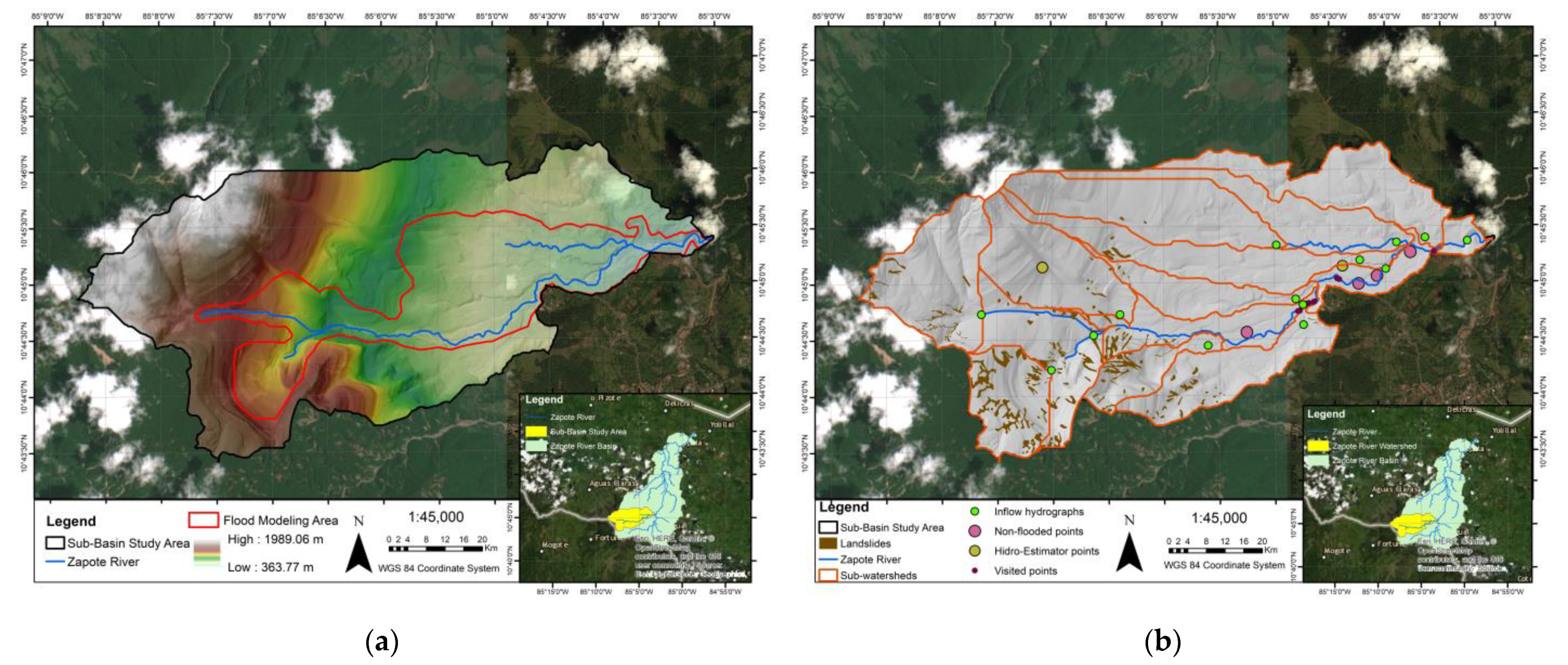
The study area is located in an upland sub-basin of the upper Zapote River Basin (205.5 km2), Upala canton, in the north of Costa Rica (Figure 1a). For hydrologic modeling and landslide quantification, the focus area is on the sub-basin (30.6 km2), and hydraulic simulations are on an area of 9.61 km2, shown as black and red polygons in Figure 1a, respectively. The area is prone to having saturated soils that, combined with meteorological events, will intensify flooding and causing landslides and other catastrophes.
In July 2016, four moderate earthquakes of magnitude 4.0 to 5.3 on the Richter scale were recorded around 4 km to 6.8 km north of Bijagua, affecting terrain stability and generating local landslides. Additionally, Hurricane Otto, a Category Two hurricane on the Saffir–Simpson scale, hit the country between 22 and 26 November 2016. Nearby weather stations reported on 24 November a total rainfall of 235 mm for Bijagua (10°43′59.952″ N, 85°3′11.844″ W), 179.8 mm for Canalete (10°50′11.22″ N, 85°2′23.64″ W), and 156.8 mm for Upala (10°52′51″ W, 85°04′21″ W). The Bijagua weather station is located about 5.4 km northwest of the sub-basin study area. Otto was the first hurricane-force cyclone that directly impacted Costa Rica since historical records began in 1851 [56].
A debris flow was triggered by landslides and extreme rainfall on the evening of 24 November 2016. Local experts indicated that volumetric movements were between 3250 to 4430 metric tons for a coverage area of approximately 7.2 hectares falling in the study area. The landslide’s depth was between 4.5 m and 7.5 m. According to Highland and Bobrowsky [57], this asseveration indicates a distance–length ratio less than 0.1, where translational landslides present a ruptured surface. A mixture of sediments, trees, and rocks fell unexpectedly in the upstream catchments and was subsequently propagated along the main channels to Upala city.
The phenomenon left damages in communities, infrastructures, telecommunications, water distribution systems, riverbeds, and agriculture. Furthermore, 10,831 people were affected directly, and 10 people died in the country. A water intake structure with a broad crested weir is located 1.1 km upstream of the sub-basin study area outlet point. The structure could not contain the material and water flowing over the weir with a dam break risk.

2.2. Methodological Outline

The methodological approach is presented in two parts: hydrology and hydraulic analysis with a post-event case study, where rainfall input sources and sediment concentrations were simulated to estimate the hazardous areas in a small ungauged watershed. Fundamental data, including terrain survey, soil analysis, rheological parameters, flood watermarks, land use classification, and rainfall data, were gathered and analyzed. A hydrograph comparison was developed to measure the behavior of each rainfall source. Several hydraulic simulations were developed using Cv and rainfall sources to estimate the best floodplain fit model. Additionally, an estimation of landslide volume was obtained.

2.3. Hydrologic Modeling

The hydrological simulation in the sub-basin study area was developed using the HEC-HMS model. The simulation required delineating and calculating sub-watershed parameters to obtain inflow hydrographs for FLO-2D hydraulic simulation. Such input parameters as areas, slopes, runoff curve numbers (CN), time of concentration, hydraulic channel characteristics for initial abstractions and infiltration, unit hydrograph, and routing processes were quantified.
The National Commission for Risk Prevention and Emergency Response of Costa Rica (CNE, spanish acronym) did a post-event photogrammetry analysis of World-View3 images (30 cm resolution, taken on 17–27 February 2017) to generate a 1 m high-resolution Digital Elevation Model (DEM). This information was used to delineate sub-watersheds and create the mesh. The sub-basin study area (30.6 km2) (Figure 1a) was divided into 14 sub-watersheds (Figure 1b) using the 1 m high-resolution DEM. Additionally, ArcGIS 10.8 and Arc-Hydro-Tools were used to calculate sub-watershed areas, slopes, elevation analysis, longest flow paths, river characteristics, and input parameters.
CN values resulted from the combination of soil map [58], land-use classification, and AMC II. The WorldView-3 images were used to generate the land use map applying a supervised image classification and user detail adjustments to refine the land use areas. Additionally, it allowed a forensic image assessment of affected areas, identifying landslides, riverbed and bank scour, and material depositional areas. The soils in the area were characterized by andisols (93.2%), inceptisols (6.13%), and ultisols (0.65%) in lower areas [58]. The andisols have a volcanic origin, high organic matter contents, hummus accumulations, medium texture, weak structures, and good to moderate drainage. A “B” hydrologic group was assigned to andisol soils.
The time of concentration for sub-watersheds was calculated using the sum of travel times of consecutive flow segments through the longest flow path, depending on flow types, such as sheet flow, shallow concentrated flow, and open channel flow [15]. The sheet flow is generated principally over surfaces. Manning’s Roughness Coefficient (Manning’s n) incorporates the effect of raindrop impact, obstacles, erosion, and sediment transport at shallow flow depths (around 3 cm and distances less than 90 m). The shallow concentrated flow is a function of the watercourse slope and type of channel. Finally, the open channel flow is applied where channels are well defined and visible on aerial photographs. Additionally, Manning’s equation is applied to bank-full elevation [15]. Natural Resources Conservation Service (NRCS) dimensionless unit hydrograph and the Muskingum–Cunge methods were applied to the hydrologic simulation, where hydraulic routing parameters were obtained from channel characteristics, DEM, aerial images, and field visits.
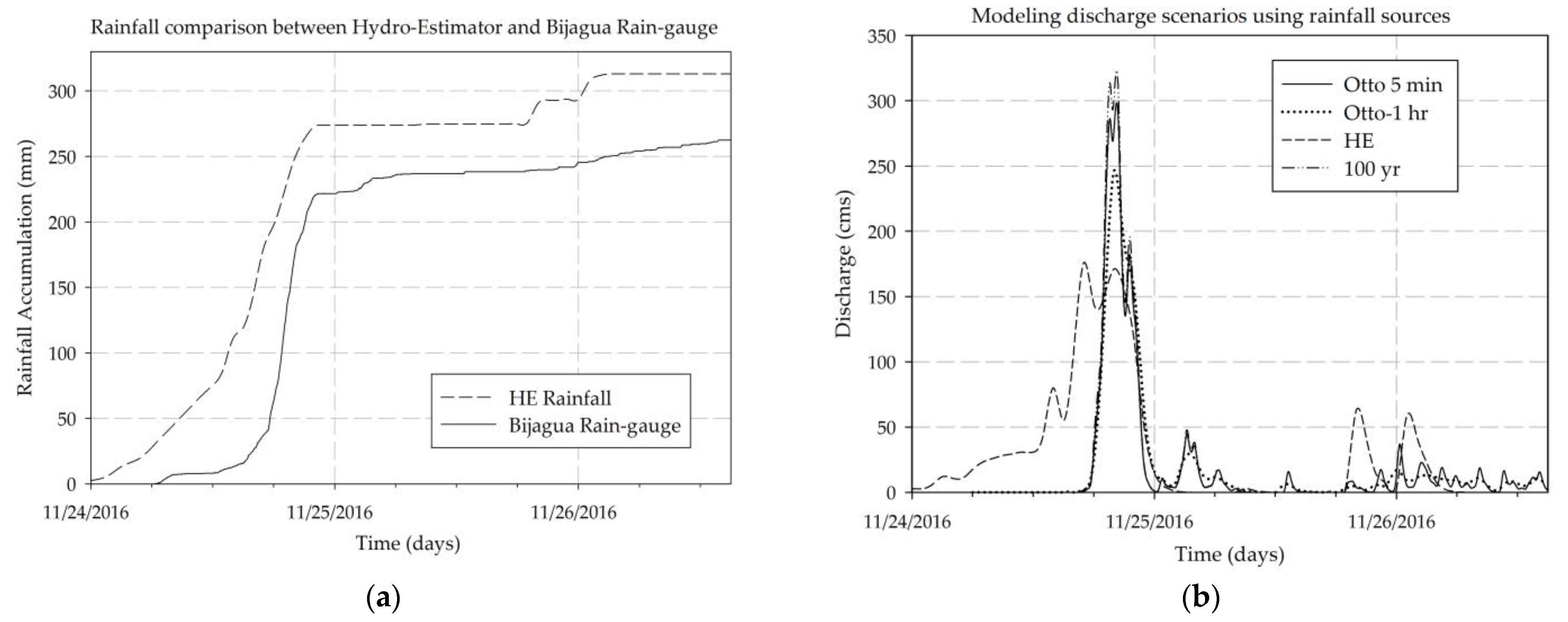
Three base scenarios were performed in HEC–HMS using several rainfall inputs to study their behavior in an upland and small mountainous sub-basin (Figure 1a). The first scenario corresponded to Hurricane Otto’s event measured by the Bijagua weather station (5 min time step); the second was a 100-year return period designed storm. The third was using QPE by Hydro-Estimator algorithm.
The hydrologic simulation for each rainfall scenario generated 14 hydrographs to be incorporated into the FLO-2D. The hydraulic analysis is described in Section 2.5. The accuracy of satellite rainfall products is vital in flood and debris flows computation in complex terrain and heavy rainfall; therefore, QPEs need to be evaluated. HE could become an essential tool for operational emergency managers, mainly when low rain gauge density or a lack of information exists.

2.3.1. Rainfall Analysis

Storms recorded in the Northern area of Costa Rica typically are caused by tropical depressions and convection storms, not by hurricanes. Therefore, no characterization of this type of meteorological phenomenon was done. Additionally, studies have not been conducted to determine the temporal distribution of designed rainfall, and only traditional synthetic methods are applied in the Region. In the absence of discharge stations, a frequency analysis of annual maximum rainfall data for Bijagua’s rain gauge was conducted to generate Depth–Duration–Frequency (DDF) curves, develop a designed storm and simulate rainfall-runoff process for 25-year, 50-year, and 100-year return period hydrographs. Durations of 5 min to 6 h were taken from 2000–2018 records, and for 24 h, the period was from 1990 to 2018. A Gumbel PDF was applied, and comparisons between Otto rainfall depths at durations of 15, 30, 60, 120, 180, 360, and 1440 min with the return periods were conducted. In terms of contrast, the event magnitude (Hurricane Otto versus 100-year return period), a 24 h temporal distribution was extracted from Otto’s event and applied to the rainfall depth of the 100-year return period.
HE data are available worldwide (www.star.nesdis.noaa.gov (accessed on 9 June 2018) [26]) in ASCII format at a 1 h temporal resolution and 4 km spatial resolution. The HE pixels information were extracted, and digital numbers ranging from 0 to 256 were converted into rainfall accumulation applying the following Equation (1).
R = (value − 2) × 0.3048
where value is an HE rainfall number, a value of 0 means missing rainfall, and a value of 2 means no rainfall.
An inverse distance method was applied to the HEC–HMS meteorological model with a search ratio of 4 km. The method calculates the mean aerial rainfall and consists of selecting the nearest HE pixel to the nearby sub-watershed centroids, assigning more weight to the rainfall time series closer to the centroid.

2.3.2. Performance Evaluation

Graphical comparison, continuous statistical and categorical evaluation were applied to quantify the rainfall performance in hydrologic simulation scenarios. The continuous statistics were evaluated using the mean bias ratio (MBR), mean absolute error (MAE), and root mean square error (RMSE) for HE and rain gauge rainfall accumulations (1 h). The MBR is a correction factor of satellite quantifications and corresponds to the relationship between rain gauge and HE rainfall accumulations for a specific period. Therefore, HE rainfall could be corrected by multiplying each pixel value by MBR for future events and enhancing the performance of hydrologic simulations with QPE. Nevertheless, the HE correction in real-time applications is challenging due to the watershed concentration times in small areas.
The categorical evaluation was estimated with a classical two-way contingency table to HE product (Table 1). Additionally, contingency table typical scores were calculated as hit rate (H), probability of detection (POD), false alarm rate (FAR), and discrete bias (DB) [59,60].
H = a + d N
POD = a a + c
FAR = b a + b
DB = a + b a + c
This study maintained the HE rainfall without MBR correction to evaluate the repercussion on hydrographs in real-time hydrological analysis, and flood depths for hydraulic applications for Newtonian and non-Newtonian flows.
The hydrographs’ performances were evaluated using the MAE, RMSE, and Nash-Sutcliffe model efficiency (NSE). NSE values around 1 indicate perfect agreement between the baseline scenario and 100-year return period at 5 min, or with HE at one-hour time resolution [61].

2.4. Landslide and Cv’s Analysis

An image analysis was performed to delineate and quantify the displaced area and estimate landslide volume, using the WorldView-3 image and assuming a translational landslide. According to Highland [57], the translational landslide’s rupture surface has a distance–length relationship of less than 0.1. It can range from minor faults (residential lot size) to large regional landslides (kilometers wide). Deep landslides are around 5 to 10 m, confirming CNE’s presumption about landslide depths.
The sediment concentration relationships (6)–(9) define the nature of hyper-concentrated sediment flows, relating the volumetric sediment concentration (Cv) (6), sediment concentration by weight (Cw), specific weight of sediment (γs), mudflow mixture specific weight (γm), and the load factor (BF) Equation (9). Therefore, it is essential to identify in situ sediment concentration either as a measure of weight or volume.
Cv = SV [ WV + SV ]
Cv = C w γ [ γ m C w ( γ s γ ) ]
γ m = γ + Cv [ γ s γ ]
BF = 1 [ 1 Cv ]
where γ is the specific weight of water, SV is sediment volume, and WV is water volume.
A Cv of 0.2 for a conventional riverbed results in a load factor of 1.25, indicating that the flood volume is 25% higher than if the clear-water flow is considered. Non-clear-water is considered when volumetric sediment concentrations are between 0.2 and 0.45.
Such rheological models as the Bringham plastic model (10) and the yield-pseudoplastic model (11) describe the relationships between shear stress and shear rate in soil materials capable of flow and hyperconcentrated flows. However, field investigations and laboratory tests need to be conducted. As in this case study, in cases in which data were not available, O’Brien [62] presented the relationships between soils and particle size tests, liquid limit, and plasticity index. Additionally, the empirical coefficients ( α 1 ,   α 2 ,   β 1 and   β 2 ) are presented for the viscosity ( η ) and yield stress ( τ y ) in Equations (12) and (13) related to Cv. Consequently, FLO-2D applies these parameters as a function of Cv [46,63]
τ = τ y +   η du dy
τ = τ y +   a   du dy n
τ y = α 1 e β 1 Cv
η = α 2 e β 2 Cv
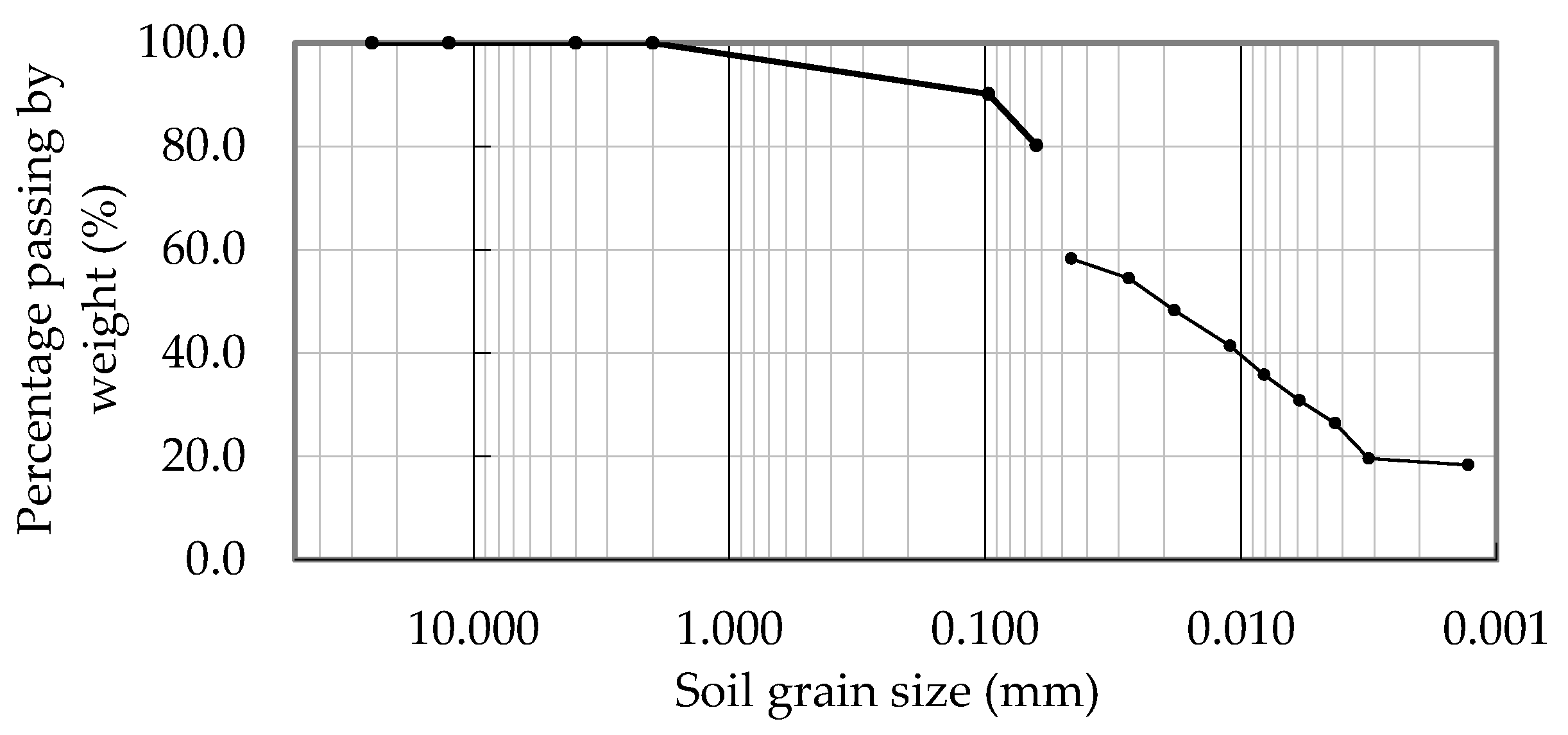
The average grain size distribution curve and Atterberg limits of in situ samplings tested post-event can approximate the soil selection in FLO-2D and the corresponding rheological parameters [62,63]. Methods such as sieving and Bouyoucos Hydrometer tests for fine materials are applied to describe the soils in the area.
The Atterberg limit test identifies soil plasticity degree, differentiating between very plastic, moderate, or non-plastic soils. Liquid limits less than 50% and plastic index greater than 7% indicate a material with clay presence. The plasticity indexes for debris flow sediment matrices greater than 5% are classified as mudflows [62]. In order to characterize the soil composition that could be dislodged during the event, soil samples were taken at different points along the riverbed, riverbanks, and landslides nearby (Figure 1b).
Granulometry tests were performed according to ASTM D422 standard [64], obtaining particle size distribution D10, D30, D60, and D80 and uniformity coefficient (CU). The plasticity tests, liquid limit, and plastic limit were performed using the procedure indicated by the ASTM D4319 standard [65]. The tests were developed in the Water, Soils, and Environment Laboratory of the Department of Biosystems Engineering at the University of Costa Rica.

2.5. Hydraulic Modeling

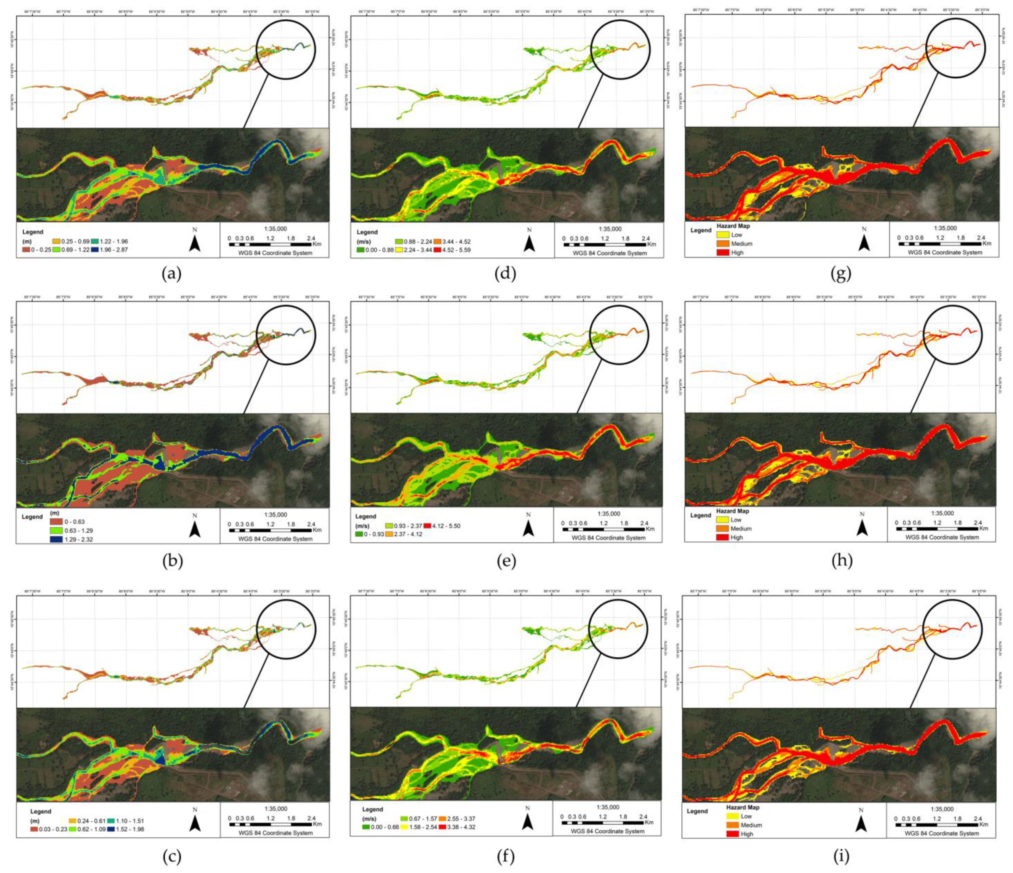
The hydraulic modeling was developed using FLO-2D to obtain flow depths, velocities, and flood hazard maps. Hydrologic scenarios were modeled for clean-water (Newtonian flow) and debris flow (non-Newtonian flow) conditions with different sediment concentrations (Cv) (0.30, 0.45, 0.55, and 0.65) to study the model sensitivity to determine the flood plain, and the most probable Cv reaching the observed flood elevations.
The FLO-2D hydraulic model requires main inputs for Newtonian and non-Newtonian flows, including a digital elevation model (DEM) to generate the modeling mesh, roughness Manning’s n values, inflows (simulated hydrographs), outflow condition, simulation time step, Courant number, Cv, and empirical coefficients for the soil ( α 1 ,   α 2 ,   β 1 and   β 2 ).
The simulated hydraulic area was about 9.61 km2 (Figure 1a) with a 5 m grid resolution (384,424 pixels). The 5 m grid was generated from a DEM resample from the original 1 m cell resolution using a cubic convolution resampling technique developed in the ArcGIS 10.8 program.
Manning’s n values were assigned to the mesh based on land use classification, following the recommendations found in [12,66,67,68] and field verification. The final values assigned to the model are shown in Table 2. An average value of 0.08 was selected for the river channel, considering soil characterization, stone size, and comparison with the bibliography mentioned, which shows similarities to the field.
The inflow hydrographs were obtained from the hydrologic modeling (HEC–HMS) using rain gauges, the HE algorithm, and the 100-year return period. Each scenario generated fourteen inflow hydrographs for each sub-watershed and applied them to the hydraulic model (FLO-2D) for clear-water and debris flow simulations. The inlet points are shown in Figure 1b. The outflow discharge nodes were simulated using critical depth flow conditions. Additionally, general considerations such as stability parameters as output time step interval of 0.1 h, simulation time of 72 h, and Courant number of 0.6 were assigned.
Debris modeling requires several extra parameters due to its non-Newtonian fluid nature. These parameters are based on the viscosity–sediment concentration and yield stress-sediment concentration empirical relationships (10–13) [62], where empirical values “α” and “β” were based on laboratory tests from Zapote’s soil samples and contrasted with Rocky Mountain samples [64] according to Section 2.4. In addition, the debris flow hydrograph was distributed according to Cv and depended on the hydrograph behavior.
Regarding hazard maps, three flood intensity categories were determined depending on velocities and depth flow product, according to the methodology developed in [69], which is included in FLO-2D [63]. Each clean-water or debris flow hazard intensity was assigned a representative color in the risk map. Red represents a severe danger to people and the destruction of physical structures. Orange represents medium danger; people are in danger outside their homes, and structures can be damaged and destroyed depending on the construction characteristics. Yellow is a low hazard; people are in very low or almost nonexistent danger, and structures may suffer minor damage, but flooding and sediment could affect the interior of homes [63].

Hydraulic Validation and Performance Evaluation

A survey was carried out in March–April 2018 to validate the model, where flood depths and flooding descriptions (arrival hour, losses) were collected with GPS in dams, bridges, rivers, and neighboring houses. RMSE and MAE were calculated to measure the accuracy between the simulations and field observations.
The hydraulic model’s performance was evaluated with the mean absolute difference (E) (14) and the measure of fit (F) (15) using the rain-gauge–clear-water scenario as the baseline to quantify the differences between Newtonian and non-Newtonian flow depths with different rainfall information sources.
E = 1 N i = 1 N | L ri L mi |
where L ri is the water depth simulated by the baseline model (rain gauge and clear-water scenario); L mi is the water depth elevation estimated by the combination of rainfall and Cv scenarios; and N is the total number of pair pixels between floodplain scenarios.
The measure of fit (F) was developed in [70] and applied in [52] to evaluate model structure sensitivity in terms of flood extend (15).
F = M 1 M 2 M 1 M 2 100
where M 1 and M 2 are the simulated and baseline flood extents, respectively; and are the intersection and union functions in ArcGIS 10.8. An F value of 100% indicates that the two floodplains are spatially precise [70]. Additionally, statistics as the mean and standard deviation of velocities and flow depths were calculated for the scenarios.

3. Results

3.1. Hydrologic Analysis for Hurricane Otto

3.1.1. Physical Characterization of the Sub-Basin

The hydrologic study area delineation resulted in fourteen small sub-watersheds, ranging between 0.37 km2 to 3.44 km2 (Figure 1b). Terrain elevation values were between 363.77 and 1989.06 m, with an average of 987.61 m and a standard deviation of 391.19 m (Figure 1). The hypsometric curve presented a median of 846 m. The most frequent altitudes were between 600 to 700 m with a relative frequency of 15.36%, followed by a 500 to 600 m range with 10.87%. The watershed presented high-terrain slope variability with an average of 30.33% (16.9°), a standard deviation of 32.18% (17.8°), and a maximum of 85.68% (40.6°). In low zones, slopes predominated around 1–9.74%. The shape factor value was 0.5. The compactness index of 1.96 indicates an elongated basin, where floods are smaller than an equal size area with a more significant shape factor. The drainage density value of 1.45 km/km2 indicated moderate drainage, slightly erodible, and very permeable soils. The average channel slope and the slope index were 8.4% (4.8°) and 1.72. Lower areas presented channel slopes ranging from 2% to 2.4%, in the middle reach from 7.1% to 7.6%, and in the upper tributaries from 10.4% to 34.5%.
The main land uses obtained were forest (55%), agriculture (13%), grassland (12%), bare soil (4%), urban (3%), and clouds (14%). The weighted CNs for AMC II were between 52.84 and 67.35, indicating good drainage and vegetation coverage according to the soil maps and land use classification mentioned in Section 2.3. Additionally, the concentration times had values between 18.37 min and 54.29 min.

3.1.2. Rainfall Analysis Results

A Gumbel PDF analysis was applied to Bijagua’s rain gauge and obtained a coefficient of determination (R2) of 0.99 with a significance level of 5% for the Depth–Duration–Frequency (DDF) curves. The PDF analysis provided the exceedance probability for different durations, and the opportunity to compare with Hurricane Otto measured with HE and rain gauge, shown in Table 3. For instance, a 100-year return period obtained 109.73 mm and 248.82 mm for rainfall durations of 120 min and 1440 min, respectively. No information was available for durations between 6 and 24 h for the DDF analysis. The rain gauge recorded a maximum rainfall depth of 236.22 mm for 24 h, allocated in the range of 50- to 100-year return period. However, Hurricane Otto rainfall occurred principally on 24 November from 06:35 to 22:20 (around 16 h), accumulating 221.5 mm. In that time, was observed the major impact.
The HE algorithm underestimated maximum rainfall depths for durations of 1 h to 3 h with a percentage error of 43.86% and 45.7%, respectively, remaining even below the 5-year return period. However, for durations greater than 6 h, they were similar to those calculated for the station. An error of 0.76% was found in 6 h and tendency to overestimate in durations of 12 h to 24 h (Table 3).
Figure 2a illustrates rainfall accumulations and timing differences between Bijagua’s rain gauge and the corresponding HE pixel. The HE rainfall detection initiated 7 h before the rain gauge. However, the end of the heaviest rainfall (23:00) had a delay of only 45 min compared to rain gauge records (22:25), less than HE time resolution. At this time, HE had a rainfall accumulation of 274.06 mm and 221.50 mm for the rain gauge, presenting an MBR of 0.81. At the end of the simulation time (26 November 15:00), the HE rainfall accumulation was 312.19 mm, and 262.55 mm for the rain gauge, presenting an MBR of 0.84.
The mean aerial HE rainfall over sub-watersheds varied from 270.12 mm to 385.33 mm, with an average in the sub-basin of 340.68 mm, for MBR of 0.88 for the same period. However, if the start time is the same as that of the rain gauge (06:00), the MBR is 0.9 (Table 3). The performance of HE is presented in Table 3, which shows different values based on durations. The H, POD, FAR, and BIAS had superior performance when the heaviest rainfall was presented, but MAE and RMSE were higher at the same durations.

3.1.3. Hydrological Results

Hydrographs obtained from HEC–HMS simulations at sub-basin outlet using HE rainfall, rain gauge at 5 min and 1 h durations, and 100-year return period designed rainfall are shown in Figure 2b. Additionally, Table 4 shows the peak flows and direct runoff volume results at the sub-basin outlet point as examples. Nonetheless, hydrographs, peak discharges, time to peak, and direct runoff volume were obtained for 14 sub-watersheds to be introduced as input boundary conditions into the hydraulic model.
The simulated Otto event using the weather station (5 min) produced two peak flows. The first peak hit the area on 24 November 2016 at 19:45 with a peak runoff of 286.2 m3/s, with an ascending curve over 130 min. The second one was triggered on 24 November 2016 at 20:15 with a maximum value of 298.3 m3/s.
The 100-year return period simulation presented the same arrival times and a maximum peak flow of 323.3 m3/s, showing a difference of 8.38% compared to the 5 min rain gauge simulation. The NSE was 0.989, presenting a good agreement in the skill and behavior of the 100-year simulation (Figure 2b). Nevertheless, the two peak flows were hidden in the 1 h hydrograph where the arrival time was 20:00 h.
The HE simulation generated the first peak of 175.9 m3/s, earlier than expected (17:00), producing differences of 41% compared to 5 min data and 28.61% for 1 h rain gauge. The HE’s second peak flow matched in time (20:00) with the peak calculated with the rain gauge, and the descending curve had a similar decrease rate. However, the NSE was 0.25 for the simulation at a 1 h rainfall resolution.

3.2. Landslide Estimation and Cv Analysis

Studies of landslide estimation and soil characterization were performed to approximate sediment concentrations and rheological parameters in hydraulic simulations. As a result, 127 landslides were detected in the upper Zapote River Basin by satellite image inspection, and 63 landslides with a displacement area of approximately 0.58 km² probably affected the study river reach. Figure 1b shows the landslide locations in the sub-basin study area. The material volume of 4 million m3 assumed a landslide depth of 5 m, and with a depth of 7 m, the contribution would be 5.76 million m3, resulting in a sediment concentration of 0.36 to 0.52.
Several granulometry tests were carried out to know the distribution of the soil in the study area, principally in the river and landslide areas shown in Figure 1b. The results showed that the granulometry corresponds to particles larger than D80 (0.063 mm), but more giant stones are in the field (0.5–2 m). Sample points such as riverbanks and riverbeds had a significant presence of silts and clays, where the fine material content varies between 57.53% and 100%. Figure 3 shows the predominant particle sizes from nearby landslide sample points. No stones or particles larger than 1 mm were found. Silts were between 0.074 mm to 0.005 mm, with a small percentage of clays (D50 is 0.023 mm, and the D90 is 0.097 mm).
The soil plasticity could not be determined since the soil did not have the necessary structure to carry out the test. This type of material had been exposed for three years after Otto’s event, which implies that most of the clay soil structures had already been removed by hydric erosion, leaving courser structures. Base on soil samples and information as shown in O’Brien and Julien [62], the “Natural Aspen Soil” was considered to be applied in FLO-2D.

3.3. Hydraulic Modeling Results for Newtonian and Non-Newtonian Flows

3.3.1. Clean-Water (Newtonian) Scenarios Evaluation

As mentioned in the previous sections, three rainfall information sources evaluated Hurricane Otto as a case study in the hydraulic model; results are shown in Figure 4. The hydraulic simulation using the Bijagua’s station (5 min time resolution) and clear-water condition, referred to as “hydraulic baseline scenario”, occasioned flow depths between 0.01 m and 2.87 m, with an average of 0.48 m and a standard deviation of 0.55 m (Figure 4a). As the channel becomes deeper and narrower, it can reach depths of more than 1.96 m to 2.87 m. Velocities (Figure 4d) are mainly between 0.01 m/s and 3.44 m/s, with an average speed of 1.52 m/s and a standard deviation of 1.48 m/s, while greater velocities up to 5.59 m/s occur in the same places where flow depth increase. The hazard map (Figure 4g) shows the product between velocities and depths in concordance with the classification exposed in [63]. The risk category was high at depths greater than 1.5 m through the channel, and the product of velocities and depths was greater than 1.5 m2/s, while in several places on the floodplain, the risk can vary between medium and low levels. The hazard categories obtained did not represent as much danger as observed during the event, where more giant stones were mobilized and generated a scour bank of 100 to 180 m in some places. The results showed that Newtonian flow average depths and velocities are insufficient to reproduce the disaster observed. Clear-water simulation was not reaching many areas that the flood covered, according to satellite photo mapping. Thus, Cv simulations are necessary to cover the observed flood plain.
The results of the 100-year design return period using rainfall distribution of Hurricane Otto showed that depths and velocities relative to hydraulic baseline scenario had similar behavior with a slight average increase of 0.04 m. The simulation can reach 2.32 m; likewise, in most flooded areas, it maintains a flow depth between 0.1 and 1.15 m (Figure 4b), and the average depth in the flood plain was 0.5 m with a standard deviation of 0.58 m. Regarding velocities, illustrated by Figure 4e, the behavior was similar to the hydraulic baseline scenario, remaining between 0.01 m/s and 4.12 m/s, with an average depth of 1.57 m/s and standard deviation of 1.52. The average differences in depth and velocities with Bijagua’s simulation were 90 cm and 1 m/s, respectively. However, a depth increase of almost one meter can significantly damage infrastructure and threaten people, as reflected in danger levels (Figure 4h).
The Hydro-Estimator simulation results showed slight differences compared to Otto. Flood depths were between 0.03 and 1.98 m, while the average depth was 0.43 m with a standard deviation of 0.5 m (Figure 4c). Velocities varied between 0.01 m/s and 4.32 m/s, with an average of 1.24 m/s and a standard deviation of 1.18 m/s (Figure 4f). This model distributed its risk in three hazard levels (Figure 4i), similar to the hydraulic baseline scenario. HE simulation increased the medium and high hazard levels of the previous simulation. The accuracy in runoff volume was more critical than peak flow in this particular floodplain. A water intake infrastructure with a broad crested weir is located at 1.1 km upstream of the outlet study area, generating material and water damming. Visual verification with Figure 4g–i demonstrated an agreement in the hazard coverage area. Only the HE product indicated slight visual differences in category levels.

3.3.2. Debris Flow Simulations

The floodplain was analyzed with debris flow using four sediment concentrations (Cv: 0.3, 0.45, 0.55, and 0.65) and the three hydrologic scenarios mentioned above. Based on granulometric curves determination in the study area, the “Aspen Natural Soil” soil type [45] was selected due to the presence of fine material and lack of plasticity to be applied as standard input in the hydraulic models.

3.3.3. Volumetric Sediment Concentration of 0.3

The debris flow analysis with a Cv of 0.3 and Otto’s rainfall resulted in an average flood depth of 1.24 m with a standard deviation of 0.942 m; 0.76 m more than the clear-water simulation, and 62% of the heights were up to 2 m. The average speed was 1.73 m/s with a standard deviation of 1.41 m/s, and 40% of its velocities were more than 4 m/s. The event’s maximum velocities generated a considerable expansion of the main channel with boulder movement of around 1 m to 2 m diameter. In terms of hazard categories, 17% of the flooded area is at medium level, while the remaining is at high hazard, destroying everything in its pathway.
The Cv of 0.3 and 100-year return period hydraulic simulation results increased hazard levels compared to Otto’s rainfall. However, the flooded average depth was smaller than the previous one with an average of 1.17 m, a standard deviation of 0.88 m/s, and a maximum depth flow of 3.67 m; 80% of the heights are between 0.01 m and 1.90 m. In addition, the average velocity was 2.16 m/s with a standard deviation of 1.69 m/s; 0.43 m/s more than Otto’s rainfall, concentrating the velocities on the third quartile. As a result, an increment in the medium hazard level category was obtained, growing from 17% to 22% of the area.

3.3.4. Volumetric Sediment Concentration of 0.45

The Cvs of 0.45 simulation results with the different input rainfalls are presented in Figure 5. Water depth results are shown in Figure 5a–c, velocities in Figure 5d–f, and hazard area delineation in Figure 5g–i. Rain gauge simulation presented an average flow depth of 1.95 m, and 86% lower than 3.04 m depth (Figure 5a). Fifty percent of the area obtained depths greater than 2 m, twelve percent more than Cv simulation of 0.3 for the same rainfall scenario. The average velocity was 1.92 m/s with a standard deviation of 1.35 m/s (Figure 5d). Only 10% of the flow was categorized as medium and 90% as high level, making it typically destructive (Figure 5g).
The 100-year return period results showed that the flooded average depth was 1.78 m with a standard deviation of 1.18 m, 46% higher than 2 m (Figure 5b). Flow velocities exhibit an average of 1.87 m/s with a standard deviation of 1.37% and a maximum of 7.80 m/s (Figure 5e). The average difference in flow depth maps was 0.41 m lower than the simulation with Bijagua’s weather station, and in the case of velocities, differences were 0.06 m/s. Likewise, 15% of the flooded area resulted in a medium level, and the remaining was high level (Figure 5h). Both simulations presented a mean absolute difference (E) of 1.72 m for rain gauge hydrologic simulation and 1.38 m for the 100-year simulation.
Hydro-estimator’s hydrological simulation presented flow depths between 0.03 m and 4.16 m with an average of 1.20 m, and a standard deviation of 1.02 m (Figure 5c). The flooded average velocity was 1.17 m/s and a standard deviation of 1.34 m/s (Figure 5f). A high level of danger corresponds to 58.76% of the floodplain, while a medium level covers 13.55% of the floodplain (Figure 5i). Therefore, a reduction in velocities and depths generated a reduction in danger and risk. These results are concordant to Cv of 0.3 and rain gauge simulation, demonstrating a depth mean absolute difference (E) of 0.715 m and an E standard deviation of 0.45 m.

3.3.5. Volumetric Sediment Concentration of 0.55

For Cv of 0.55, there was a significant change in the results compared to the previous hydraulic modelings. The average flow depth obtained was 3.38 m with a standard deviation of 1.83 m, and 68% of flow depths are more significant than 2 m, making it extremely dangerous. Like the previous cases, the average velocity was 1.88 m/s with a standard deviation of 1.3 m/s; nevertheless, as flow depth and velocity increased, the high hazard level increased to 98%.
The simulation using a 100-year return period showed similar results to the rain gauge simulation, where flow depths greater than 2 m encompassed 75% of the total flooded area. The average flow depth was 3.6 m with a standard deviation of 2.05 m. An average velocity of 1.84 m/s was attained with a standard deviation of 1.4 m/s. The average differences between rain gauge and 100-year return period floodplain maps were 0.35 m in depths and 0.036 m/s in velocities.

3.3.6. Volumetric Sediment Concentration of 0.65

The Cv of 0.65 for rain gauge simulation obtained the highest average depth compared to previous Cv results, with an average depth of 5.52 m and a standard deviation of 4.06 m. The 100-year return period simulation results indicated an average depth of 5.71 m with a standard deviation of 4.38 m. Simulated flow depths could rise to 20.25 m and velocities up to 9.96 m/s, principally at inlet cells. The flow becomes greater than 2 m throughout the whole channel. The velocities obtained from the 100-year return period also remain at an average of 2.02 m/s with a standard deviation of 1.97 m/s. The hazard level in both simulations was 100% high-level. At sediment concentration above 0.6, the fluid begins to lose debris flow properties and presents more sliding properties.

3.4. Hydraulic Model Validation and Performance Evaluation

Hydraulic model validation was developed by comparing high-resolution satellite post-event photos, modeling depth results, and water benchmarks in the floodplain. A destroyed bridge near the town of Zapote left people isolated. A flood height of 3.3 m was necessary to overpass the bridge abutments and the roadway surface. The channel width pre-event was around 14 m and post-event was expanded to 134 m, generating a lateral scour of 120 meters’ width. Another critical point for the evaluation was a water intake structure located 1.1 km upstream from the outlet point, where a flood depth of 2.2 m was measured. The floodplain generated upstream to the broad-crested spillway had around 300 m width, whereas the channel in the pre-event condition had only 20 m. Table 5 presents the in situ depths measured and the simulated depths for Cvs. The MAE and RMSE showed that Cv of 0.45 presented lower values (0.51 m and 0.98 m, respectively). However, Cv of 0.3 presents the second-lowest error. Additionally, Cv of 0.45 generated an entrance of 2.95 million m3 landslide volume, and for Cv of 0.55, 3.95 million m3, which was closer to that estimated by CNE.
Table 6 shows flow depth mean absolute differences (E), a measure of fit (F), and E standard deviation between sediment-concentration-hydrologic model scenarios compared to the hydraulic baseline scenario (rain gauge and clear-water condition). Results indicated significant flow depth differences and floodplain extent match between hydraulic scenarios with non-Newtonian (Cv) and Newtonian flows (clear-water). However, the E, F, and E standard deviations between rain gauge and 100-year return period simulations were very similar for Cv scenarios.
HE simulation for clear-water presented similar behavior to the baseline scenario and 100-year return period for all performance measurements, an E of 0.092 m in flow depths was found (Table 6). Only a slight reduction in F was found, demonstrating a value greater than 90%. An increment of Cv values from 0.3 to 0.45 demonstrated that the HE floodplain was similar to the simulated Cv of 0.3. The E was less than 4.5 cm, and F of 84.92% versus 87.96% for the rain gauge simulation; additionally, the E standard deviation differences were 5 cm between models (Table 6).
The Cv simulation of 0.55 generated more significant differences in E and F between rain gauge and 100-year hydraulic simulations than the baseline scenario. Hazard mapping resulted in almost 100% high level. No significant differences were found in flow depth maps between rain gauge and 100-year return period simulations with the hydraulic baseline scenario, as were shown in Table 6. The mean absolute differences (E) were 2.95 m and 3.32, respectively. The Cv of 0.65 presented an E of 5.19 m for the rain gauge hydraulic simulation and 5.48 m for the 100-year model. The F values presented differences of 58.98% and 55.04%, respectively, demonstrating a significant change compared to the clear-water flood plain results.

4. Discussion

Many factors, including earthquakes, extreme events, hurricanes, steepness, and saturated soils, can combine and trigger debris flows in small upland watersheds, especially in the Zapote Basin (November 2016). The landslide was approximately 3.25 million cubic meters, assuming a 5 m depth and a translational displacement of material according to the CNE and recommendations in [57]. The main upland channel was scoured and widened, generating changes from 14 m up to 300 m. Debris flow mapping was developed in a case study in an upland sub-basin (Figure 1a) with high terrain slope variability (16.87° of average slope), and mean channel slopes of 4.8°. Other studies had satisfactory results for the same slopes [38,39,40,41,42]. However, limitations and uncertainties existed to predict runoff, especially in applying the runoff CN method to tropical watersheds. Typical CN values suggested in the literature were applied to the high-resolution land use classification, indicating well-drained areas. However, investigations presented a poor performance in basins dominated by subsurface runoff and suggested reducing the initial abstraction ratio from a typical 0.2 value to 0.045 [16,17]. The CN effects are directly propagated to peak flow and runoff volume, affecting the hydraulic results.
Hurricane Otto presented lower maximum rainfall depths than a 5-year return period for durations less than one hour. Nonetheless, the depth increased almost to the 100-year return period for a 24 h duration. A gap in the annual maximum intensity records for durations between 3 h and 24 h was identified in the DDF, so it is impossible to characterize the event between these durations. However, Hurricane Otto hit the area with greater force over 6 h, generating a significant ascending hydrograph curve of 130 min duration.
It is challenging to have a high-density rain gauge network that represents accurate precipitation in mountainous tropical watersheds. QPE products have been evaluated in mountainous areas [21,30,71,72], and the accuracy depends on the cloud system type, cloud-top temperature, QPE resolution, and topography. HE detection differences identified in this study were probably generated by cloudiness in front of the hurricane’s eye, and threshold brightness temperature in the HE algorithm that detects rainfall. In addition, clouds in tropical zones are warmer than those in subtropical areas, reducing HE detection capacity, such as indicated in [30,59] and underestimating rainfall rate [25]. Additionally, HE presented elevation-dependent biases [30], characterized by underestimation in the occurrence of light precipitation at high elevations. However, HE tended to overestimate precipitation at durations over 24 h, as indicated in [25]. Further, MBR must be calculated at sub-daily time resolution to avoid incorrect HE corrections.
The HE hydrologic results showed a total runoff volume of 15.75%, more than rain gauge hydrologic simulation and lower peak flows. HE rainfall distribution in the first eight hours and lower rain rates propitiated the infiltration process and mitigated the peak flows.
The rainfall time resolution in the hydrological modeling was an essential factor in the accuracy of peak flow estimation. An increase in time step from 5 min to 1 h generated a reduction in the maximum peak flows and concealment of the consecutive peaks in a time window of 30 min. Thus, rainfall accumulation differences of 5.33% turned into 8.38% in maximum peak flows as mentioned in [32,73].
Higher velocities than erosion and transport critical velocity for sediment sizes up to 15 mm (corresponding to pebbles according to the Hjulström diagram [74,75]) generated river and bank erosion and scour.
In ungauged watersheds, Manning’s n selection for the floodplain needs to be meticulous, and it is necessary to have accurate ground cover information. Lin et al. [13] indicated that Manning’s n significantly affected the debris-flow processes.
Debris flow presented three main areas as suggested by [49]: a source area with slopes greater than 20° (where mass starts accelerating); a transport zone (channel), where the volume increased by entrainment of material and flow and reached terminal velocity (slopes steeper than 15–20° to generate a velocity where erosion occurs); and a depositional area with channel slopes of 1 to 9°.
The rheological parameters found in the literature [62] and the ones estimated by density curves from soil samples generated the opportunity to choose suitable rheological values in the model. However, Chow et al. [4] considered that rheology calculated from soil samples generates much higher agreement in modeled results than the reported in the literature.
The HE product in the hydraulic simulation demonstrated a worthy approximation of flooded areas affected by extreme events with clear-water, where a lack of rainfall information and complex terrain exists. It is challenging to predict the landslide volume and collect field-based data during real-time meteorological applications. Only when possible landslide failure is mapped and monitored could risk be estimated in advance. However, a Cv increment could compensate the floodplain depth reduction in debris flow modeling.
Cv from 0.3 to 0.65 generated high velocities combined with high water depths, especially at input grid cells, where higher debris flow concentration exists. However, the Cv of 0.65 had more sliding behavior than debris flow, especially at input nodes.
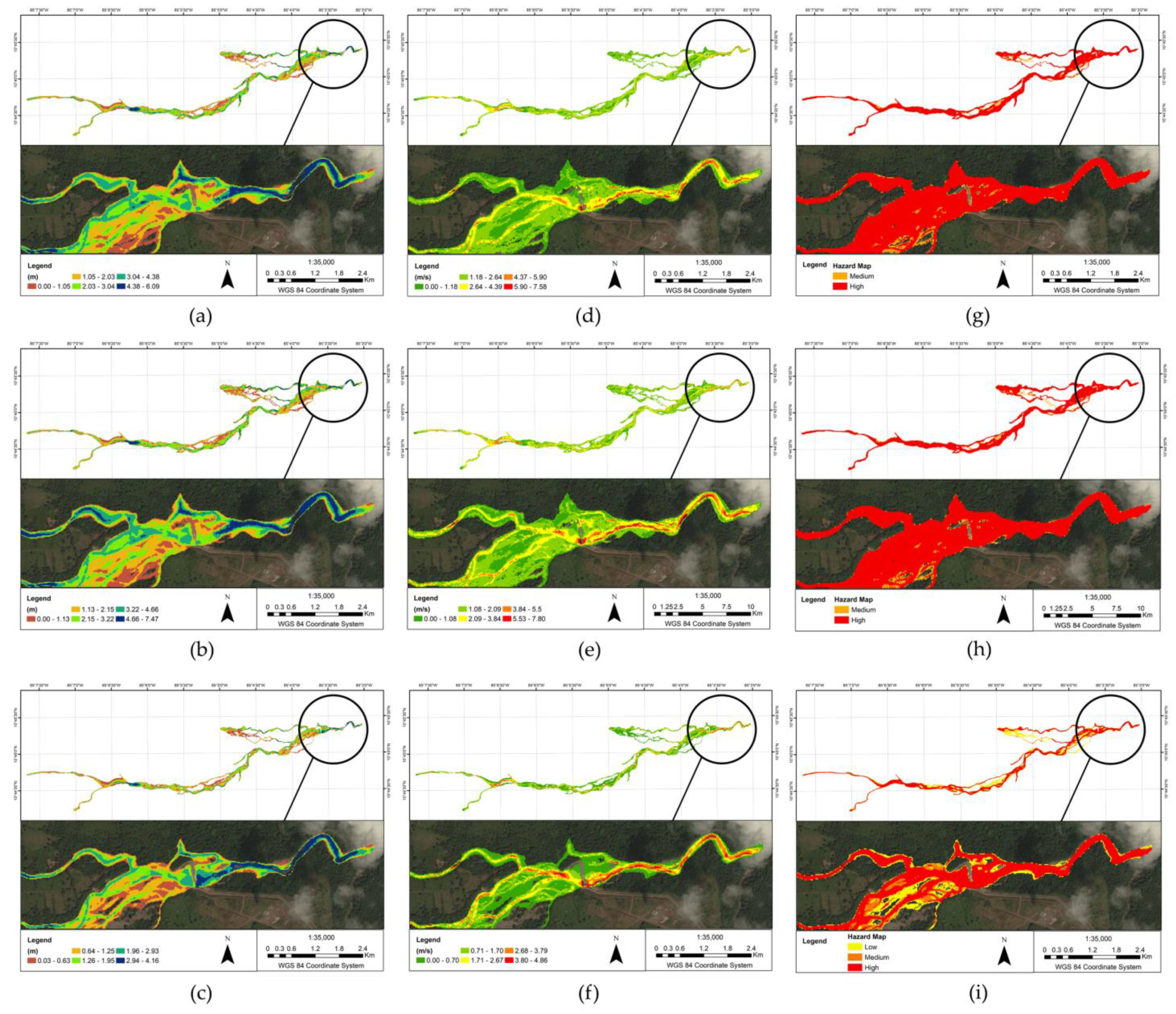
The clear-water spatial patterns found in Figure 4 between hydrologic scenarios followed a similar behavior to the E and F analysis (Table 6). The average flow depths and standard deviations in the hydraulic modeling area presented no significant differences between rainfall events. The broad crested spillway at 1.1 km from the outlet sub-basin study area retained the water–material mixture while the spillway was over-flooded. This condition generated an attenuation in flow depths and velocities upstream.
No significant differences were found between E and F for the debris flow hydraulic simulations with rain gauge station and 100-year return period. The spatial patterns addressed in Figure 5a,b evidenced the findings. A mean increase in flood zone depths of 0.8 m, 1.93 m, 3.36 m, and 5.52 m were calculated for Cv of 0.3, 0.45, 0.55, and 0.65 compared to the hydraulic baseline scenario.
The same behavior was found in HE simulations with a tendency to increase the flood area (8.28 ha), as shown in Figure 4i and Figure 5i. In addition, the sensitivity analysis demonstrated that the Cv is the most important parameter for debris flow computation [4]. Therefore, debris mapping and real-time floodplain estimates would be utilized in the emergency management and flood alert systems to minimize risk using possible Cv based on historical estimations.

5. Conclusions

In 2016, northern Costa Rica suffered destruction from Hurricane Otto. The destruction was mainly by debris flows provoked by heavy rainfalls on mountainous areas. Therefore, a methodology was implemented to map the flooded areas in ungauged small upland watersheds byapplying recorded rainfall and satellite rainfall quantifications (HE) and different sediment concentrations (Cv) in a post-event hydrologic-hydraulic approach.
The Hydro-Estimator algorithm overestimated rainfall accumulations (MBR of 0.8) for the 24 h duration and runoff volume by 15.7% compared to the rain gauge modeling at the outlet point. Nevertheless, the peak discharges were 41% lower than those simulated with the rain gauge station at 5 min and 28.6% lower than the one-hour resolution. HE generated an attenuation of peak discharges, presenting two significant peaks. The first peak was 45 min in advance of Otto’s hydrograph, less than HE time resolution, but the second peak matched it in time. The descending hydrograph curve between rainfall products presented a good agreement with Otto’s hydrograph.
HE MBR at sub-daily time resolution would enhance the rainfall estimates and flood predictions for future events in ungauged mountainous watersheds.
FLO-2D was capable of reproducing Hurricane Otto’s floodplain with different sediment concentrations. The flood depths and velocities for clean-water conditions were not enough to capture the flood plain cover. It showed the necessity to include sediment concentrations that could increase flow depths, velocities, transport boulders, and cover the disaster area.
The verification of the hydraulic model applying visual verification of aerial photography and site flow depth measurements showed acceptable results with sediment concentration values ranging from 0.35 to 0.45. It has been shown that increasing sediment concentration in the channel generated significant differences in flow depths between Cv scenarios. However, mean absolute differences less than 0.5 m were achieved between hydraulic scenarios (Cvs) where a 5.3% rainfall difference exists.
HE demonstrated a good performance in clear-water conditions. The HE uncertainties in the hydraulic simulation were compensated with rainfall volume overestimation, generating no significant differences in flow depth maps for clean-water (Newtonian flow) simulations because a downstream broad-crested spillway generated mitigation of maximum flow depths.
Sediment volume concentration affected the amplification of debris flow, depths, velocities, and hazard levels. Results showed that it is recommendable to continue using hydrologic and two-dimensional models in upland and ungauged tropical watersheds to delineate probable debris flood hazard areas. However, this recommendation is limited to adequate soil representation for rheological characterization, high-resolution DEM, and photography of affected areas.
HE rainfall product with MBR corrections at the sub-daily time scale can reproduce clear-water, and debris flow analysis in a river with a spillway near the outlet. Additionally, when a lack of rainfall information exists or the watershed is located in a remote place, HE can be helpful in strategies for risk prevention and flood alert systems.

Author Contributions

Conceptualization, S.F.S. and A.M.R.G.; Data curation, S.F.S.; Formal analysis, S.F.S. and A.M.R.G.; Funding acquisition, A.M.R.G.; Investigation, S.F.S.; Methodology, S.F.S. and A.M.R.G.; Project administration, A.M.R.G.; Resources, A.M.R.G.; Supervision, A.M.R.G.; Validation, S.F.S.; Visualization, S.F.S.; Writing—original draft, S.F.S.; Writing—review and editing, A.M.R.G. Both authors have read and agreed to the published version of the manuscript.

Funding

This work was supported by University of Costa Rica (340-B7522) and the Costa Rica’s National Commission for Risk Prevention and Emergency Response (CNE) (project number 340-B7522).

Institutional Review Board Statement

Not applicable.

Informed Consent Statement

Not applicable.

Data Availability Statement

Restrictions apply to the availability of these data. Data were obtained from Costa Rica’s National Commission for Risk Prevention and Emergency Respondse (CNE) and Costa Rican Electricity Institute (ICE) and are available from the authors with CNE and ICE permissions.

Acknowledgments

We thank the Costa Rica´s National Commission for Risk Prevention and Emergency Response (CNE) for their collaboration in this study, providing helpful feedback, topography and high-resolution satellite imagery.

Conflicts of Interest

The authors declare no conflict of interest.

References

  1. Centre for Research on the Epidemiology of Disasters. EM-DAT|The International Disasters Database. Available online: https://www.emdat.be/ (accessed on 14 June 2021).
  2. UNISDR (United Nations Office for Disaster Risk Reduction). DesInventar Open Source Initiative. Available online: https://www.desinventar.net/ (accessed on 14 June 2021).
  3. Banihabib, M.E.; Jurik, L.; Kazemi, M.S.; Soltani, J.; Tanhapour, M. A Hybrid Intelligence Model for the Prediction of the Peak Flow of Debris Floods. Water 2020, 12, 2246. [Google Scholar] [CrossRef]
  4. Chow, C.; Ramirez, J.; Keiler, M. Application of Sensitivity Analysis for Process Model Calibration of Natural Hazards. Geosciences 2018, 8, 218. [Google Scholar] [CrossRef] [Green Version]
  5. D’Agostino, V.; Tecca, P.R. Some Considerations on the Application of the FLO-2D Model for Debris Flow Hazard Assessment. In Monitoring, Simulation, Prevention and Remediation of Dense and Debris Flows; Lorenzini, G., Brebbia, C.A., Emmanoulouloudis, D.E., Eds.; WIT Press: Southampton, UK, 2006; Volume 90, pp. 159–170. ISBN 1845641698. [Google Scholar]
  6. Hsu, S.M.; Chiou, L.B.; Lin, G.F.; Chao, C.H.; Wen, H.Y.; Ku, C.Y. Applications of Simulation Technique on Debris-Flow Hazard Zone Delineation: A Case Study in Hualien County, Taiwan. Nat. Hazards Earth Syst. Sci. 2010, 10, 535–545. [Google Scholar] [CrossRef] [Green Version]
  7. Liu, W.C.; Hsieh, T.H.; Liu, H.M. Flood Risk Assessment in Urban Areas of Southern Taiwan. Sustainability 2021, 13, 3180. [Google Scholar] [CrossRef]
  8. Petroselli, A.; Vojtek, M.; Vojteková, J. Flood Mapping in Small Ungauged Basins: A Comparison of Different Approaches for Two Case Studies in Slovakia. Hydrol. Res. 2019, 50, 379–392. [Google Scholar] [CrossRef] [Green Version]
  9. Yadav, M.; Wagener, T.; Gupta, H. Regionalization of Constraints on Expected Watershed Response Behavior for Improved Predictions in Ungauged Basins. Adv. Water Resour. 2007, 30, 1756–1774. [Google Scholar] [CrossRef]
  10. Gumindoga, W.; Rwasoka, D.T.; Nhapi, I.; Dube, T. Ungauged Runoff Simulation in Upper Manyame Catchment, Zimbabwe: Application of the HEC-HMS Model. Phys. Chem. Earth 2017, 100, 371–382. [Google Scholar] [CrossRef]
  11. Annis, A.; Nardi, F.; Petroselli, A.; Apollonio, C.; Arcangeletti, E.; Tauro, F.; Belli, C.; Bianconi, R.; Grimaldi, S. UAV-DEMs for Small-Scale Flood Hazard Mapping. Water 2020, 12, 1717. [Google Scholar] [CrossRef]
  12. Sarchani, S.; Seiradakis, K.; Coulibaly, P.; Tsanis, I. Flood Inundation Mapping in an Ungauged Basin. Water 2020, 12, 1532. [Google Scholar] [CrossRef]
  13. Lin, P.S.; Lee, J.H.; Chang, C.W. Application of the FLO-2D Model to Debris-Flow Simulation. A Case Study of Song-Her District in Taiwan. In Proceedings of the 5th International Conference on Debris-Flow Hazards Mitigation: Mechanics, Prediction and Assessment, Padua, Italy, 14–17 June 2011; Genevois, R., Hamilton, D.L., Prestininzi, A., Eds.; Casa Editrice Università La Sapienza: Roma, Italic, 2011; Volume 8, pp. 947–956. [Google Scholar]
  14. Quan Luna, B.; Blahut, J.; Van Westen, C.J.; Sterlacchini, S.; Van Asch, T.W.J.; Akbas, S.O. The Application of Numerical Debris Flow Modelling for the Generation of Physical Vulnerability Curves. Nat. Hazards Earth Syst. Sci. 2011, 11, 2047–2060. [Google Scholar] [CrossRef] [Green Version]
  15. United States Department of Agriculture Urban. Hydrology for Small Watersheds; Technical Release 55; United States Department of Agriculture: Washington, DC, USA, 1986.
  16. Valle, L.C.G.D.; Rodrigues, D.B.B.; de Oliveira, P.T.S. Initial Abstraction Ratio and Curve Number Estimation Using Rainfall and Runoff Data from a Tropical Watershed. Rev. Bras. Resur. Hidricos. 2019, 24, 1–5. [Google Scholar] [CrossRef] [Green Version]
  17. Woodward, D.E.; Hawkins, R.H.; Jiang, R.; Hjelmfelt, A.T., Jr.; Van Mullem, J.A.; Quan, Q.D. Runoff Curve Number Method: Examination of the Initial Abstraction Ratio. In Proceedings of the World Water & Environmental Resources Congress 2003, Philadelphia, PA, USA, 23–26 June 2003; Bizer, P., DeBarry, P., Eds.; American Society of Civil Engineers: Reston, VA, USA; pp. 1–10. [Google Scholar]
  18. Granato, G.E. Estimating Basin Lagtime and Hydrograph-Timing Indexes Used to Characterize Stormflows for Runoff-Quality Analysis; Scientific Investigations Report 2012–5110; U.S Geological Survey: Reston, VA, USA, 2012. [Google Scholar]
  19. Grimaldi, S.; Kao, S.C.; Castellarin, A.; Papalexiou, S.M.; Viglione, A.; Laio, F.; Aksoy, H.; Gedikli, A. Statistical Hydrology. In Treatise on Water Science; Wilderer, P., Ed.; Elsevier, B.V.: Amsterdam, The Netherlands, 2011; Volume 2, pp. 479–517. ISBN 9780444531995. [Google Scholar]
  20. Rojas González, A.M.; Harmsen, E.W.; Pol, S.C. Performance Evaluation of MPE Rainfall Product at Hourly and Daily Temporal Resolution within a Hydro-Estimator Pixel. WSEAS Trans. Environ. Dev. 2009, 5, 478–487. [Google Scholar]
  21. Dos Reis, J.B.C.; Rennó, C.D.; Lopes, E.S.S. Validation of Satellite Rainfall Products over a Mountainous Watershed in a Humid Subtropical Climate Region of Brazil. Remote Sens. 2017, 9, 1240. [Google Scholar] [CrossRef] [Green Version]
  22. Habib, E.; Aduvala, A.V.; Meselhe, E.A. Analysis of Radar-Rainfall Error Characteristics and Implications for Streamflow Simulation Uncertainty. Hydrol. Sci. J. 2008, 53, 568–587. [Google Scholar] [CrossRef]
  23. Rojas González, A.M. Flood Prediction Limitations in Small Watersheds: Bias Estimation in Radar Precipitation Product. In Flood Assessment: Modeling and Parameterization; Harmsen, E.W., Goyal, M.R., Eds.; Apple Academic Press: Toronto, NJ, USA, 2018; ISBN 9781315365923. [Google Scholar]
  24. Vieux, B.E.; Bedient, P.B. Assessing Urban Hydrologic Prediction Accuracy Through Event Reconstruction. J. Hydrol. 2004, 299, 217–236. [Google Scholar] [CrossRef]
  25. Scofield, R.A.; Kuligowski, R.J. Status and Outlook of Operational Satellite Precipitation Algorithms for Extreme-Precipitation Events. Weather Forecast. 2003, 18, 1037–1051. [Google Scholar] [CrossRef] [Green Version]
  26. NOAA-NESDIS. STAR Satellite Rainfall Estimates Hydro-Estimator Digital Global Data Archive. Available online: https://www.star.nesdis.noaa.gov/smcd/emb/ff/digGlobalData.php (accessed on 9 June 2018).
  27. Scofield, R.A. The NESDIS Operational Convective Precipitation- Estimation Technique. Mon. Weather Rev. 1987, 115, 1773–1793. [Google Scholar] [CrossRef]
  28. Vicente, G.A.; Davenport, J.C.; Scofield, R.A. The Role of Orographic and Parallax Corrections on Real Time High Resolution Satellite Rainfall Rate Distribution. Int. J. Remote Sens. 2002, 23, 221–230. [Google Scholar] [CrossRef]
  29. Joyce, R.; Janowiak, J.; Huffman, G. Latitudinally and Seasonally Dependent Zenith-Angle Corrections for Geostationary Satellite IR Brightness Temperatures. J. Appl. Meteorol. 2001, 40, 689–703. [Google Scholar] [CrossRef]
  30. Yucel, I.; Kuligowski, R.J.; Gochis, D.J. Evaluating the Hydro-Estimator Satellite Rainfall Algorithm over a Mountainous Region. Int. J. Remote Sens. 2011, 32, 7315–7342. [Google Scholar] [CrossRef]
  31. de Siqueira, R.A.; Vila, D. Hybrid Methodology for Precipitation Estimation Using Hydro-Estimator over Brazil. Int. J. Remote Sens. 2019, 40, 4244–4263. [Google Scholar] [CrossRef]
  32. Yucel, I. Assessment of a Flash Flood Event Using Different Precipitation Datasets. Nat. Hazards 2015, 79, 1889–1911. [Google Scholar] [CrossRef]
  33. Demissie, M.; Keefer, L.; Lian, Y.; Yue, F.; Larson, B. Hydrologic and Hydraulic Modeling and Analyses for the Cache River for the Purposes of Evaluating Current Conditions and Alternative Restoration Measures; Contract Report 2008-01; Illinois Department of Natural Resources: Springfield, IL, USA, 2008.
  34. Balmforth, N.J.; Craster, R.V. Geophysical Aspects of Non-Newtonian Fluid Mechanics. In Geomorphological Fluid Mechanics; Balmforth, N.J., Provenzale, A., Eds.; Springer: Berlin/Heidelberg, Germany, 2007; Volume 582, pp. 34–51. ISBN 978-3-540-45670-4. [Google Scholar]
  35. Iverson, R.M. The Physics of Debris Flows. Rev. Geophys. 1997, 35, 245–296. [Google Scholar] [CrossRef] [Green Version]
  36. Di Santolo, A.S.; Pellegrino, A.M.; Evangelista, A. Experimental Study on the Rheological Behaviour of Debris Flow. Nat. Hazards Earth Syst. Sci. 2010, 10, 2507–2514. [Google Scholar] [CrossRef]
  37. Jakob, M. Debris-Flow Hazard Analysis. In Debris-Fow Hazards and Related Phenomena; Jakob, M., Hungr, O., Eds.; Springer: Berlin/Heidelberg, Germany, 2005; pp. 411–443. ISBN 978-3-540-27129-1. [Google Scholar]
  38. Prochaska, A.B.; Santi, P.M.; Higgins, J.D.; Cannon, S.H. Debris-Flow Runout Predictions Based on the Average Channel Slope (ACS). Eng. Geol. 2008, 98, 29–40. [Google Scholar] [CrossRef]
  39. Pierson, T.C. Dominant Particle Support Mechanisms in Debris Flows at Mt Thomas, New Zealand, and Implications for Flow Mobility. Sedimentology 1981, 28, 49–60. [Google Scholar] [CrossRef]
  40. Broscoe, A.J.; Thomson, S. Observations on an Alpine Mudflow, Steele Creek, Yukon. Can. J. Earth Sci. 1969, 6, 219–229. [Google Scholar] [CrossRef]
  41. Sharp, R.P.; Nobles, L.H. Mudflow of 1941 at Wrightwood, Southern California. Bull. Geol. Soc. Am. 1953, 64, 547–560. [Google Scholar] [CrossRef]
  42. Barman, P.C.; Kairi, R.R.; Das, A.; Islam, M.R. An Overview of Non-Newtonian Fluid. Int. J. Appl. Sci. Eng. 2016, 4, 97–101. [Google Scholar] [CrossRef]
  43. Takahashi, T. Debris Flow: Mechanics, Prediction and Countermeasures, 2nd ed.; CRC Press, Taylor and Francis Group: London, UK, 2014. [Google Scholar]
  44. UK GeoHazards. Landslides Classification. Available online: http://www.ukgeohazards.info/pages/eng_geol/landslide_geohazard/eng_geol_landslides_classification.htm (accessed on 9 June 2021).
  45. O’Brien, J.S.; Julien, P.Y.; Fullerton, W.T. Two-Dimensional Water Flood and Mudflow Simulation. J. Hydraul. Eng. 1993, 119, 244–261. [Google Scholar] [CrossRef]
  46. FLO-2D Pro. Reference Manual. Available online: https://flo-2d.com/downloads/ (accessed on 6 February 2019).
  47. Mergili, M.; Fellin, W.; Moreiras, S.M.; Stötter, J. Simulation of Debris Flows in the Central Andes Based on Open Source GIS: Possibilities, Limitations, and Parameter Sensitivity. Nat. Hazards 2012, 61, 1051–1081. [Google Scholar] [CrossRef] [Green Version]
  48. Wu, Y.H.; Liu, K.F.; Chen, Y.C. Comparison between FLO-2D and Debris-2D on the Application of Assessment of Granular Debris Flow Hazards with Case Study. J. Mt. Sci. 2013, 10, 293–304. [Google Scholar] [CrossRef]
  49. Frekhaug, M.H. An Assessment of Prediction Tools to Norwegian Debris Flows, Norwegian University of Science and Technology; NTNU: Trondheim, Sweden, 2015. [Google Scholar]
  50. Cesca, M.; D’Agostino, V. Comparison between FLO-2D and RAMMS in Debris-Flow Modelling: A Case Study in the Dolomites. In Monitoring, Simulation, Prevention and Remediation of Dense Debris Flows II; Wrachien, D., Brebbia, C.A., Lenzi, M.A., Eds.; WIT Press: Southampton, UK, 2008; Volume 60, pp. 197–206. ISBN 9781845641184. [Google Scholar]
  51. Peng, S.H.; Lu, S.C. FLO-2D Simulation of Mudflow Caused by Large Landslide due to Extremely Heavy Rainfall in Southeastern Taiwan during Typhoon Morakot. J. Mt. Sci. 2013, 10, 207–218. [Google Scholar] [CrossRef]
  52. Pinos, J.; Timbe, L. Performance Assessment of Two-Dimensional Hydraulic Models for Generation of Flood Inundation Maps in Mountain River Basins. Water Sci. Eng. 2019, 12, 11–18. [Google Scholar] [CrossRef]
  53. Jarquin Murillo, M.F. Análisis del Tránsito de Avenidas ante la Posibilidad de un Deslizamiento en el Cerro Tapezco Mediante el uso del modelo Hidráulico FLDWAV; Universidad de Costa Rica: San José, Costa Rica, 2001. [Google Scholar]
  54. Comité Regional de Recursos Hidráulicos (CRRH). El Clima, su Variabilidad y Cambio Climático en Costa Rica; Instituto Meteorológico Nacional (IMN): San José, Costa Rica, 2008. [Google Scholar]
  55. Fick, S.E.; Hijmans, R.J. WorldClim 2: New 1-km Spatial Resolution Climate Surfaces for Global Land Areas. Int. J. Climatol. 2017, 37, 4302–4315. [Google Scholar] [CrossRef]
  56. Instituto Meteorológico Nacional. Huracán Otto Informe Técnico; Instituto Meteorológico Nacional: San José, Costa Rica, 2016. [Google Scholar]
  57. Highland, L.; Bobrowsky, P. The Landslide Handbook—A Guide to Understanding Landslides; Circular 1325; U.S. Geological Survey: Reston, VA, USA, 2008.
  58. Centro de Investigaciones Agronómicas (CIA). Mapa Digital de Suelos de Costa Rica. Available online: http://www.cia.ucr.ac.cr/?page_id=139 (accessed on 9 June 2019).
  59. Ramirez-Beltran, N.D.; Kuligowski, R.J.; Harmsen, E.W.; Castro, J.M.; Cruz-Pol, S.; Cardona, M.J. Rainfall Estimation from Convective Storms Using the Hydro-Estimator and NEXRAD. WSEAS Traans. Syst. 2008, 7, 1016–1027. [Google Scholar]
  60. Mantas, V.M.; Liu, Z.; Caro, C.; Pereira, A.J.S.C. Validation of TRMM Multi-Satellite Precipitation Analysis (TMPA) Products in the Peruvian Andes. Atmos. Res. 2015, 163, 132–145. [Google Scholar] [CrossRef]
  61. Moriasi, D.N.; Arnold, J.G.; Van Liew, M.W.; Bingner, R.L.; Harmel, R.D.; Veith, T.L. Model Evaluation Guidelines for Systematic Quantification of Accuracy in Watershed Simulations. Trans. ASABE 2007, 50, 885–900. [Google Scholar] [CrossRef]
  62. O’Brien, J.S.; Julien, P.Y. Laboratory Analysis of Mudflow Properties. J. Hydraul. Eng. 1988, 114, 877–887. [Google Scholar] [CrossRef] [Green Version]
  63. Mapper Manual Pro. Available online: https://flo-2d.com/downloads/ (accessed on 7 February 2019).
  64. ASTM D422-63(2007)e2, Standard Test Method for Particle-Size Analysis of Soils (Withdrawn 2016). Available online: https://www.astm.org/Standards/D422 (accessed on 14 June 2019).
  65. ASTM D4319-93(2001), Standard Test Method for Distribution Ratios by the Short-Term Batch Method (Withdrawn 2007). Available online: https://www.astm.org/Standards/D4319.htm (accessed on 14 June 2019).
  66. Chow, V.T. Open-Channel Hydraulics; McGraw-Hill: New York, NY, USA, 1959. [Google Scholar]
  67. Barnes, H.H. Roughness Characteristics of Natural Channels; Water Supply Paper 1849; U.S. Geological Survey: Denver, CO, USA, 1987. [Google Scholar]
  68. Arcement, G.J.; Schneider, V.R. Guide for Selecting Manning’s Roughness Coefficients for Natural Channels and Flood Plains; Water Supply Paper 2339; U.S Geological Survey: Denver, CO, USA, 1989.
  69. García-Martínez, R.; López, J.L. Debris Flows of December 1999 in Venezuela. In Debris-Flow Hazards and Related Phenomena; Jakob, M., Hungr, O., Eds.; Springer: Berlin/Heidelberg, Germany, 2005; pp. 519–538. ISBN 978-3-540-27129-1. [Google Scholar]
  70. Bates, P.D.; De Roo, A.P.J. A Simple Raster-Based Model for Flood Inundation Simulation. J. Hydrol. 2000, 236, 54–77. [Google Scholar] [CrossRef]
  71. Blacutt, L.A.; Herdies, D.L.; de Gonçalves, L.G.G.; Vila, D.A.; Andrade, M. Precipitation Comparison for the CFSR, MERRA, TRMM3B42 and Combined Scheme Datasets in Bolivia. Atmos. Res. 2015, 163, 117–131. [Google Scholar] [CrossRef] [Green Version]
  72. Takido, K.; Valeriano, O.C.S.; Ryo, M.; Tanuma, K.; Ushio, T.; Kubota, T. Spatiotemporal Evaluation of the Gauge-Adjusted Global Satellite Mapping of Precipitation at the Basin Scale. J. Meteorol. Soc. Jpn. 2016, 94, 185–195. [Google Scholar] [CrossRef] [Green Version]
  73. Palmeira, F.L.B.; Morales, C.A.; França, G.B.; Landau, L. Rainfall Estimation Using Satellite Data for Paraíba do Sul Basin (Brazil). In Proceedings of the XXth International Society for Photogrammetry and Remote Sensing Congress, Technical Commission VII, Istambul, Turkey, 12–23 July 2004; Altan, O., Ed.; International Society for Photogrammetry and Remote Sensing: Hannover, Germany; pp. 1257–1262. [Google Scholar]
  74. Hjulström, F. Transportation of Detritus by Moving Water. In Recent Marine Sediment, A Symposium; Trask, P.D., Ed.; American Association of Petroleum Geologist: Tulsa, OK, USA, 1939; pp. 5–31. [Google Scholar]
  75. Woldegiorgis, B.T.; Van Griensven, A.; Bauwens, W. Explicit Incipient Motion of Cohesive and Non-Cohesive Sediments Using Simple Hydraulics. Int. Assoc. Sedimentol. 2018, 4, 78–89. [Google Scholar] [CrossRef] [Green Version]
Figure 1. (a) Sub-basin study (black polygon) and flood modeling (red polygon) areas, topography, and river location; (b) sub-watersheds, landslides detected by satellite image, inflow hydrograph, and measurement points.
Hydrology 08 00122 g001
Figure 2. (a) Rainfall accumulation comparison between Hydro-Estimator and Bijagua’s rain gauge; (b) Hurricane Otto hydrographs for Bijagua’s rain gauge at 5 min and 1 h, 100-year return period; and Hydro-Estimator rainfall.
Hydrology 08 00122 g002
Figure 3. Granulometry test result for a landslide sample.
Hydrology 08 00122 g003
Figure 4. Maps for clean-water modeling for Hurricane Otto using a rain gauge, 100-year return period, and Hydro-Estimator: (ac) flood depth maps, (df) flood velocity maps, (gi) flood hazard maps.
Hydrology 08 00122 g004
Figure 5. Flood maps results for debris flow simulation using a Cv of 0.45 and rainfall sources as the rain gauge, 100-year return period, and Hydro-Estimator: (ac) flood depth maps, (df) flood velocity maps, (gi) flood hazard maps.
Hydrology 08 00122 g005
Table 1. Contingency table example to evaluate HE performance at hourly scale. The fields of a, b, c, d represent the total number (N) of data pairs meeting the conditions.
Observed Rainfall (Rain Gauge)
YesNo
Estimated rainfall (HE)Yesab
Nocd
Table 2. Manning’s n values for different land use in the sub-basin study area.
Land UseAverage Manning’s nLocal Channel Post-Event
Agriculture 0.037 Hydrology 08 00122 i001
Forest0.123
Pastureland0.033
Bare ground: stones0.048
Channel0.080
Table 3. Depth–Duration–Frequency for Bijagua’s rain gauge, maximum rainfall depths for Otto measure by rain gauge and HE and HE performance metrics.
Return PeriodDuration (min)
51015306012018072010801440
Precipitation Depth (mm)
5-year12.2121.5528.5745.6964.3388.89111.76--151.58
10-year13.523.7931.5250.1970.58101.48131.79--175.12
25-year15.1326.6235.2555.8878.48117.38157.1--204.86
50-year16.3428.7238.0260.184.34129.18175.88--226.92
100-year17.5430.840.7764.390.15140.9194.51--248.82
Otto-Bijagua6.3512.1917.7834.5462.99109.73144.27214.38221.74236.22
Otto-HE----35.3660.6678.33212.75256.34274.02
HE performance metrics
DateMFBHPODFARDBMAE (mm)RMSE (mm)
24 November 2016, 06:00 to 23:000.900.891.000.111.1311.8214.42
24 November 2016, 06:00 to 26 November 2016, 15:000.900.580.510.150.604.678.38
Table 4. Summary results from hydrologic simulations for each rainfall scenario considered.
ScenarioRainfall Volume
(mm)
Peak Flow
(m3/s)
Direct Runoff Volume
(mm)
Time to Peak
Otto-Station 5 min 1 286.2-24 November 2016 19:35
262.55298.3145.2324 November 2016 20:15
Otto-Station 1 h 1262.55246.4145.3424 November 2016 20:00
Hydro-Estimator 1340.68 3175.9199.3524 November 2016 17:00
-171.2-24 November 2016 20:00
25-year 2204.86237.285.05-
50-year 2226.92279.8101.67-
100-year 2 313.7 24 November 2016 19:35
248.82323.3119.2624 November 2016 20:15
1 Duration registered (24 November 2016, 00:00 to 26 November 2016, 15:00). 2 24-h event duration. 3 Weighted rainfall over the watershed.
Table 5. In situ depths compared to FLO-2D flow depths.
Location
ID0123Old BridgeActual BridgeMachine HouseNear Spillway
In situ flow depth (m)00003.34.82.22
CvSimulated Flow Depths (m)MAE (m)RMSE (m)
0.30000.742.434.480.30.31.690.99
0.4500.950.361.073.284.50.450.450.510.98
0.5503.022.281.93.586.220.550.554.721.76
0.6503.932.754.3510.637.490.650.6524.553.66
Table 6. Evaluation of model’s performance between sediment concentration scenarios (Cv) and hydraulic baseline (rain-gauge-clear-water) depth simulation.
E (m)/FE Standard Deviation (m)
CvRain Gauge100-YearHERain Gauge100-YearHE
Clear-Water-0.04/96.320.092/93.83-0.050.091
0.30.76/87.960.72/87.32-0.500.44-
0.451.72/73.271.38/78.170.715/84.920.940.810.45
0.552.95/65.233.32/60.20-1.551.77-
0.655.19/58.985.48/55.04-3.954.29-
Publisher’s Note: MDPI stays neutral with regard to jurisdictional claims in published maps and institutional affiliations.

