Article

Flood Impacts on Critical Infrastructure in a Coastal Floodplain in Western Puerto Rico during Hurricane María

by
Said A. Mejia Manrique
1,*,
Eric W. Harmsen
2,*,
Reza M. Khanbilvardi
1 and
Jorge E. González
3
1
Department of Civil Engineering, The City College of New York, New York, NY 10031, USA
2
Department of Agricultural and Biosystems Engineering, University of Puerto Rico, Mayaguez 00681, Puerto Rico
3
Department of Mechanical Engineering, The City College of New York, New York, NY 10031, USA
*
Authors to whom correspondence should be addressed.
Hydrology 2021, 8(3), 104; https://doi.org/10.3390/hydrology8030104
Submission received: 8 June 2021 / Revised: 4 July 2021 / Accepted: 6 July 2021 / Published: 13 July 2021
(This article belongs to the Special Issue Hydrology in the Caribbean Basin)

Abstract

:
Flooding during extreme weather events damages critical infrastructure, property, and threatens lives. Hurricane María devastated Puerto Rico (PR) on 20 September 2017. Sixty-four deaths were directly attributable to the flooding. This paper describes the development of a hydrologic model using the Gridded Surface Subsurface Hydrologic Analysis (GSSHA), capable of simulating flood depth and extent for the Añasco coastal flood plain in Western PR. The purpose of the study was to develop a numerical model to simulate flooding from extreme weather events and to evaluate the impacts on critical infrastructure and communities; Hurricane María is used as a case study. GSSHA was calibrated for Irma, a Category 3 hurricane, which struck the northeastern corner of the island on 7 September 2017, two weeks before Hurricane María. The upper Añasco watershed was calibrated using United States Geological Survey (USGS) stream discharge data. The model was validated using a storm of similar magnitude on 11–13 December 2007. Owing to the damage sustained by PR’s WSR-88D weather radar during Hurricane María, rainfall was estimated in this study using the Weather Research Forecast (WRF) model. Flooding in the coastal floodplain during Hurricane María was simulated using three methods: (1) Use of observed discharge hydrograph from the upper watershed as an inflow boundary condition for the coastal floodplain area, along with the WRF rainfall in the coastal flood plain; (2) Use of WRF rainfall to simulate runoff in the upper watershed and coastal flood plain; and (3) Similar to approach (2), except the use of bias-corrected WRF rainfall. Flooding results were compared with forty-two values of flood depth obtained during face-to-face interviews with residents of the affected communities. Impacts on critical infrastructure (water, electric, and public schools) were evaluated, assuming any structure exposed to 20 cm or more of flooding would sustain damage. Calibration equations were also used to improve flood depth estimates. Our model included the influence of storm surge, which we found to have a minimal effect on flood depths within the study area. Water infrastructure was more severely impacted by flooding than electrical infrastructure. From these findings, we conclude that the model developed in this study can be used with sufficient accuracy to identify infrastructure affected by future flooding events.

1. Introduction

Worldwide, floods affect more people than any other natural disaster, costing $104 billion annually on average [1]. Harmsen and Goyal [2] cited several historically significant floods that resulted in extreme loss of life, for example, 12,000 lives lost in China in floods in 1980, 1996, and 1998, 30,000 in Venezuela in 1999, 2600 in Haiti in 2004, 2379 in Bangladesh in 1988, 2311 in Somalia in 1997, and 2001 in India in 1994. Other references to flood impacts are presented by [1,3,4]. Nicholls et al. [5] describe various impacts caused by flooding as direct and indirect, immediate and long-term, and tangible and intangible. The latter impact (intangible) is not often taken into account and can include psychological effects of the loss of loved ones, displacement, and property damage.
In addition to threatening human life, flooding also impacts critical infrastructure. The U.S. Department of Homeland Security (DHS) defines critical infrastructure as the “vast network of highways, connecting bridges and tunnels, railways, utilities and buildings necessary to maintain normalcy in daily life.” [6]. Electricity, water, commerce, and transportation rely on these vital systems. Failure of critical infrastructure (CI) can lead to severe economic and social disruption. CI is especially prone to flood damage [7]. Although usually not considered, natural infrastructure, defined as the coastal and marine, freshwater, and forest resources, is recognized as critical to the health and functioning of a region [8]. The National Oceanic and Atmospheric Administration (NOAA) encourages green or nature-based infrastructure as part of disaster planning and mitigation [9].
Most flood protection efforts have focused on household property and less on the protection of CI [7]. Plant et al. [10] reported a CI network analysis case study for the flooding in the Thames catchment, England. They introduced the concept of direct and indirect customer disruption estimates. The CI could be exposed to disruption by direct flooding or indirectly to dependencies of the infrastructure on the affected electrical network. Their case study describes how the interdependent infrastructure footprint extends well beyond the flooded area and across multiple governance boundaries. Numerous studies have attempted to develop strategies for enhancing the resilience of CI. Several studies have been conducted to assess the impacts on critical infrastructure to assist policymakers in prioritizing resources for recovery and hardening of CI (e.g., [11,12,13,14,15,16]).

1.1. Background

When Hurricane María hit Puerto Rico (PR) in September 2017, most large and small powerlines were knocked down. Eighty percent of the island’s electrical and communication systems were destroyed [17,18]. Downed powerlines and landslides made roads impassable for weeks or even months in specific locations. The water utility was not prepared for the hurricane and lacked power generators for running pumps. Water intakes on rivers were damaged due to extensive river meandering and sedimentation. Wastewater treatment facilities were damaged, resulting in the release of raw sewage into the floodwaters. The dam at the Guajataca Reservoir in northwest PR was severely damaged, threatening flash flooding and leaving the population without water for many months. As a consequence of the devastation of Hurricane María, the Joint Operational Catastrophic Incident Plan of PR [19] was developed. The plan represented the input from thirty State agencies, four Federal agencies, and representatives of the private critical infrastructure sectors.
The threat of flooding has increased with the relentless advance of climate change. The number of record-breaking precipitation events has increased by 12 percent between 1981 and 2010 [14]. Georgescu et al. [20] used WRF to dynamically downscale future mid- and end-of-Century rainfall patterns across the United States, focusing on the effect of weather and rainfall on metropolitan areas.
The study concluded that urban areas could expect to receive more extreme weather events and consequent increased flooding risk in the future. In general, the Caribbean region has a well-documented warming trend [21], and it is expected to experience a drying climate in the future [22], combined with more extreme rainfall [4] and drought-related events. Recently, however, Jury [23], using high-resolution satellite and reanalysis products, has hypothesized that mountainous island environments may become wetter in the future, which could lead to greater flood risk in some Caribbean island watersheds. Flooding on Caribbean islands will become aggravated with increasing sea-level rise from a warming climate. Díaz et al. [22] reported that sea levels have been rising along the coast of PR at a rate of 2 mm year−1 during the 20th Century. However, during the 2000s, the rate has increased by approximately a factor of 3. According to Hunter [24], the frequency of coastal flooding will treble for every 0.1 m rise in sea level. This implies that with a 0.5 m rise in sea level, the 1-in-100-year flood, a common recurrence interval used for the design of CI, will occur every few months.

1.2. Flood Prediction Modelling

Flood prediction models can be used to evaluate numerous factors that influence the depth and extent of flooding; factors such as land cover [25], which account for roughness and infiltration characteristics, rainfall distribution and timing [26], and compounding effects of high tide, sea-level rise, storm surge, and fluvial flooding [27,28,29]. Models can also evaluate the damage caused by flooding [25,30]. Various approaches have been used to simulate flooding. The authors of [25] used ICONOS-2 imagery to develop an improved land roughness map for the Netherlands. The LISFLOOD-FP model was used to simulate flooding based on the new land cover map. A method was described to create property damage maps, which was applied to the 1995 flood in the southern part of The Netherlands. The authors noted that the flood damage maps are helpful for decision-makers and insurance companies. Various approaches are used for representing rainfall in the hydrologic/flood models. The authors of [26] developed a SWAT model for the Polomet river basin in northwest Russia. They performed simulations with rain gauge, radar, and gauge-adjusted radar data. Comparing the observed and simulated hydrographs, the model performed best for the rain gauge, gauge-adjusted radar data, and radar, in that order. The authors of [31] provide a comprehensive overview of compound flood models in low-gradient coastal watersheds. The authors of [27] proposed a bivariate flood hazard assessment approach accounting for river flooding combined with elevated sea level, based on greenhouse gas concentration pathways 4.5 and 8.5 for 2030 and 2050. The authors of [28] developed the first compound flooding model for PR (see also [32]). They used the Gridded Surface Subsurface Hydrologic Analysis (GSSHA) model coupled with the Simulating Waves Nearshore (SWAN) and Advanced Circulation (ADCIRC) models to predict the combination of storm surge and surface runoff along the eastern coast of PR during Hurricane George. Although the storm surge and peak runoff did not coincide, the combined processes did aggravate flooding.
Numerous studies around the world have performed flood prediction modelling, applying various approaches; a few examples include Taiwan [33], UK [34], Southern Louisiana, USA [35], India, Bay of Bengal [36], the Netherlands [25], Port Hedlund, Port Phillip Bay, Australia [37], Bangladesh [38], Northern Vietnam [39], Central Caucasus, Russia [40], and Chao Phraya River Basin, Thailand [41].

1.3. Previous Hydrologic Studies Conducted in Puerto Rico

Several hydrologic studies have been conducted in the Añasco watershed, including [42,43,44,45,46]. Prieto [42] developed a surface water/groundwater MIKESHE model for the Añasco, Yagüez, and Guanajibo watersheds. The surface and subsurface conceptual and numerical models and GIS database resulted in a greater understanding of the complexities of these systems in western PR. Rojas Gonzalez [43] (also [2]) performed an upscaling experiment with the Vflo model [47] in PR to determine how the model grid spacing could be made coarser using the same parameter settings without loss of accuracy. She found, based on a stochastic analysis using the Generalized Likelihood Uncertainty Estimation (GLUE, [48]) methodology, that the 10 m hydrologic model resolution can be upscaled to 100 m resolution without loss of accuracy and that the 100 m rainfall resolution can be upscaled to 1000 m without loss of accuracy. Using the coarser grid resolution, improved model computation efficiency can be achieved. Torres Molina [44] (also [2]) evaluated short-term rainfall estimates in western PR, derived from a high-resolution radar (TropiNet, [49]) and stochastic analysis within the Mayaguez Bay drainage basin. The model served as a potential prototype for predicting real-time flooding using the Vflo model.
Ramos and Gilbes [45] developed a Soil Water Assessment Tool (SWAT) model for the Añasco watershed. The study’s main objective was to simulate runoff and sediment yields within the watershed and sediment transport to the coastal waters from 1998 to 2012. Neither the hydrologic model nor the sediment transport model were calibrated. Nevertheless, the hydrologic model was able to capture 50 percent of the variability of the observed discharge. The study showed a clear connection between coffee farms and their practices and urbanization with large sediment plumes in the coastal waters near the mouth of the Añasco River. Nilawar et al. [46] estimated soil moisture in the Añasco and Guanajibo watersheds using the SWAT model, comparing the AMSR2 soil moisture product results. The SWAT model was calibrated for 2010–2012 using USGS stream gauge data from the two watersheds. The authors concluded that SWAT fusion with AMSR2 soil moisture data can simulate streamflow in the two watersheds.
Several other hydrologic modelling studies have been conducted in PR for conditions similar to those considered in this study, including [28,50,51,52,53,54,55,56]. The authors of [50] developed a real-time runoff model to evaluate runoff for the Loíza Basin in northeast PR. Water from this basin is captured in the Carraizo reservoir and constitutes the primary water source for the San Juan metropolitan area. The model was based on estimating excess rainfall using the Green-Ampt infiltration equation. Hydraulic routing was accomplished using the HYDRAUX model [57], which solves the unsteady one-dimensional discharge in a network of open channels. The authors of [51] simulated streamflow for the Loíza Basin to characterize forecast uncertainties and statistical measures of model performance as part of a National Weather Service experiment in the Distributed Model Intercomparison Project [58]. The authors of [53] applied the Water Supply Stress Index (WaSSI) model [54] at the Luquillo National Rainforest in northeast PR. WaSSI estimates the monthly runoff volume and routed water exiting a watershed outlet. The authors of [52] applied the Hydrologic Simulation Program–FORTRAN (HSPF) to a Río Caonillas watershed in north-central PR. The three-year analysis goal was to better understand the hydrology, soil erosion, and sediment transport of the watershed. Another purpose of the study was to evaluate the ability of HSPF to perform under the PR’s extreme conditions (e.g., rainfall intensities greater than 25 mm h−1 and average slopes of 38%). The model successfully captured 85% of the monthly streamflow variability and 75% of the monthly suspended sediment concentration variability.
The authors of [55] used the Global Land Data Assimilation System (GLDAS) Noah Land Surface model to evaluate differences in pre-and post-Hurricane María hydrology over PR. GLDAS simulates overland and subsurface runoff based on 3 h and monthly increments. The study revealed that the widespread removal of leaf cover by Hurricane María resulted in elevated sediment losses for months after the passing of the hurricane. The study also showed that Hurricane María caused a change in the atmosphere’s thermodynamic structure and consequently affected cloud development and rainfall. As noted in the previous section, [28] developed a GSSHA model to simulate compound flooding in eastern PR during Hurricane George. The authors of [56] describe the Geostationary Operational Environmental Satellite Puerto Rico Water and Energy Balance (GOES-PRWEB) model. The operational model provides twenty-five hydro-agro-climate variables at a 1 km spatial resolution daily. Monthly and annual averages and totals are also available online (https://pragwater.com). The authors of [56] describe several applications of the model, including monitoring of the 2014–2016 drought in PR [59], evaluation of irrigation requirements for a 7-day period for a sweet pepper crop in southern PR, and an analysis of aquifer recharge in PR’s southern coastal aquifer from 2009–2020. Soil saturation data from GOES-PRWEB was used to initialize soil saturation values in this study.

1.4. Study Objective

The objective of this study is to develop a methodology to quantify flood conditions from extreme weather events and their impacts on critical infrastructure. As a case study, a flood inundation model is applied to the Añasco coastal flood plain of western PR. The model simulates fluvial flooding and the effect of sea rise due to storm surge. Geographic Information System (GIS) methods are used to identify potentially damaged critical infrastructure due to flooding. This study is part of a more extensive NSF-funded study to establish a framework to evaluate and enhance critical infrastructure resiliency in islanded communities. Output from the model will be incorporated into a water/power network model to assess recovery scenarios under extreme weather events.

2. Case Study Description

This section presents a short description of the effects of Hurricane María on PR and some characteristics of the study area such as location, land use land cover, and soil type distribution, among others.

2.1. Hurricane María

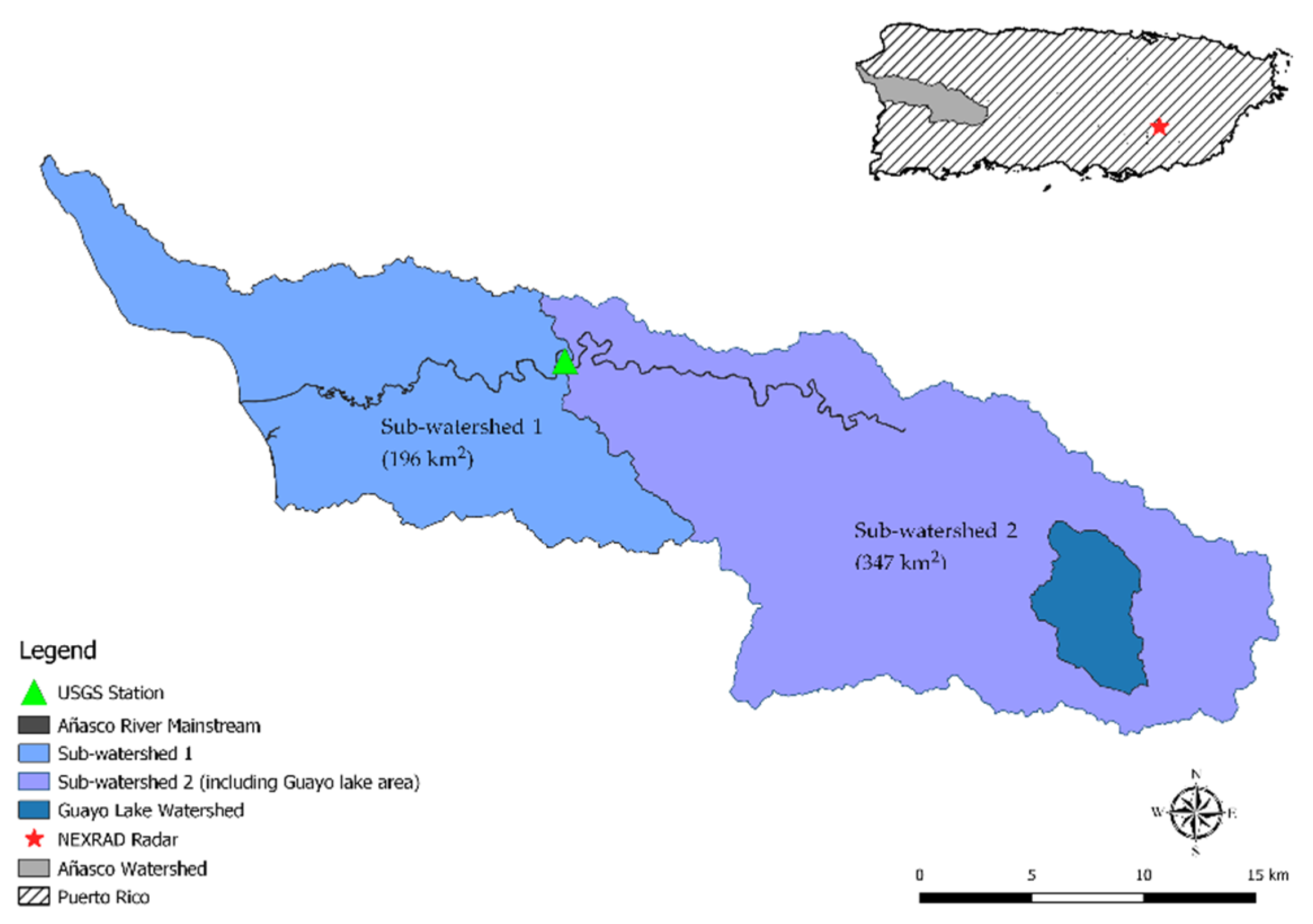
Puerto Rico is located in a susceptible zone affected by hurricanes and tropical storms (Figure 1). On 7 September 2017, Hurricane Irma hit northeast PR as a Category 3 hurricane. The eyewall passed just above the northeast corner of PR. Just 14 days later, Hurricane María passed over PR, entering the southeast corner and exiting from the northwest. Hurricane María was a Category 4 when it passed over PR on 20 September 2017 [60]. The maximum sustained wind speed was 69.3 m s−1 (249.5 km h−1) and the heavy precipitation produced serious flooding and mudslides. One of the locations in PR had a storm total of almost 38 inches (965 mm) [61]. The neutral El Niño Southern Oscillation (ENSO) and unusually high sea surface temperature (SSTs) in 2017 [62] contributed to the strength of Hurricane María. Glenn et al. [21] have observed a 0.015 °C year−1 rise in SSTs per decade in the Caribbean region between 1982 and 2012, suggesting that the conditions that enhanced Hurricane María will increase in the future.
According to the National Weather Service, in 2017, there were 64 flood-related fatalities in PR, while only 2.3 on average from 2010 to 2020 (not including 2017). For comparison, Texas reported 70 flood-related fatalities during 2017 related to Hurricane Harvey. The total estimated Hurricane María damages in PR were $90 billion [60], making it the third most costly hurricane in U.S. history, after Hurricanes Katrina and Harvey.

2.2. Study Area

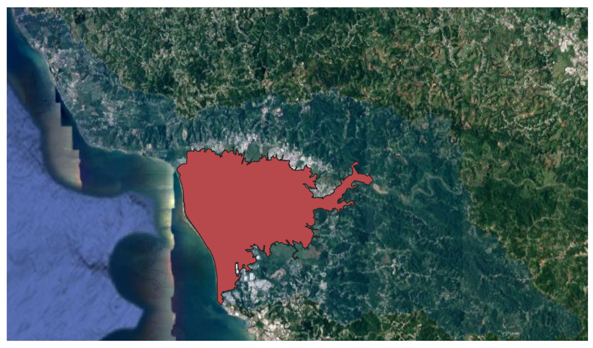
The study area is the Añasco watershed, which is located in Western PR within the municipalities of Añasco, Las Marías, Maricao, Lares, and Adjuntas. The watershed (Figure 2) is composed of a wide diversity of conditions, including urban, agriculture, and forest landscapes, topographic relief of over 1000 m, a river course with extreme meander, and a sizeable coastal flood plain, part of which includes marshland. There are four interconnected lakes located in the upper part of the watershed (Lagos Toro, Prieto, Guayo, and Yahuecas), which transfer water to southwest PR, except during extreme rainfall, when the water is released into the lower Añasco Watershed. A U.S. Geological Survey stream discharge gauge is available within the watershed, which is used to calibrate and validate the hydrologic parameters in this study. The stream discharge gauge is located in San Sabastian, PR (USGS-50144000); however, no gauges are available in the watershed’s coastal flood plain portion. The annual average rainfall in this watershed is 2160 mm. Average, minimum, and maximum yearly air temperatures are 26.1, 18.9, and 37.2 °C, respectively.
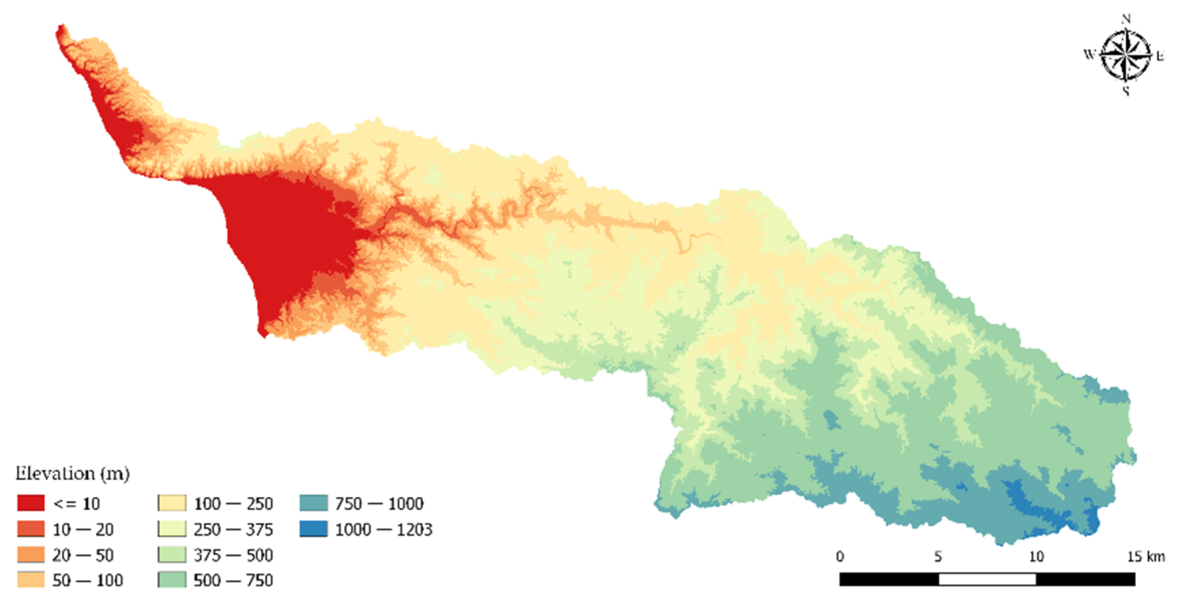
In order to reproduce the flooding during Hurricane María in this study, it was necessary to calibrate and validate some of the hydrologic parameters of the watershed; therefore, the watershed was divided into two areas, as shown in Figure 2. Sub-watershed 2 represents the region above the USGS stream discharge gauge, which was used to calibrate and validate the hydrologic parameters (essentially roughness and infiltration parameters). Subsequently, Sub-watershed 1 was used to evaluate the flooding using the calibrated parameters obtained in Sub-watershed 2. Figure 3 shows the variation of the elevations within the Añasco watershed, ranging from 0 to 1203 m above sea level. The rainfall event selected to calibrate the model was Hurricane Irma which happened days before Hurricane María, and a similar rainfall event which occurred in 2007 was selected to validate the results (this will be explained in more detail in the methodology section). It is worth mentioning that the raster precipitation data for those two events were obtained from the Next Generation Radar (NEXRAD), known as Weather Surveillance Radar 1988 Doppler (WSR-88D), which is located at 18°06′56.16″ N−66°04′41.03″ W. The star symbol in Figure 2 represents the location of the radar in PR.

Land Use Land Cover and Soil Distribution

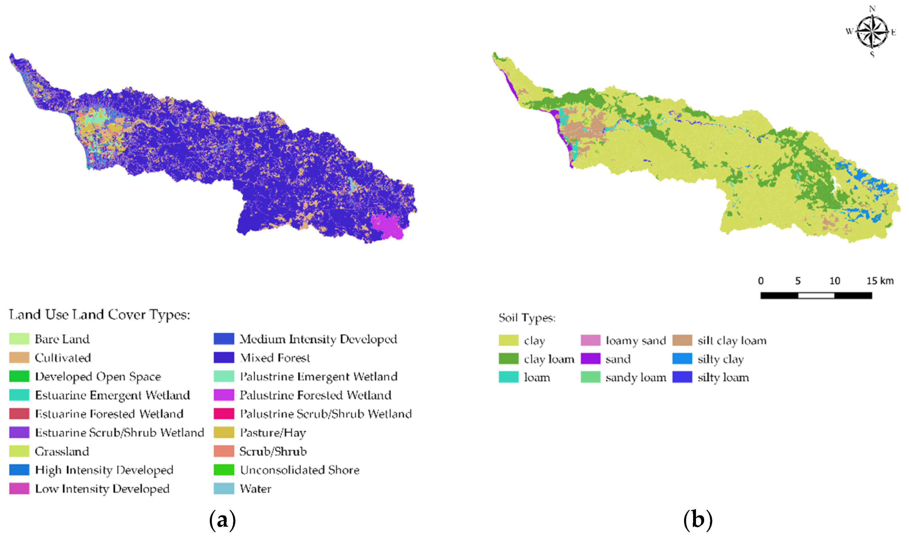
Land use land cover and soil dataset maps are essential for hydrologic simulations, allowing the association of land and soil properties into the model, such as roughness values, hydraulic conductivity, porosity, capillary head, and field capacity. Figure 4a shows the 30 m resolution land use land cover map for 2010 [63]. It was the most recent high-resolution land use land cover classification map developed for PR. The predominant land cover categories for the study area are Mixed Forest, Cultivated, and Low Intensity Developed Areas. On the other hand, Figure 4b shows the Soil Survey Geographic Dataset (SSURGO) over the Añasco watershed, which was acquired from the United States Department of Agriculture (USDA [64]). For this dataset, Clay and Clay Loam are the most representative soil categories in the Añasco watershed.

3. Methodology

The following chart (Figure 5) summarizes the main steps used in this study:

3.1. Hydrologic Model

The GSSHA is a process-based model, developed by the U.S. Army Engineer Research and Development Center (ERDC) Coastal and Hydraulics Laboratory (CHL), and is a multidimensional model that couples overland, surface, and subsurface flow. GSSHA simulates two-dimensional (2D) overland and groundwater flow, one dimension (1D) streamflow, and soil moisture [65]. A feature of GSSHA is the inclusion of spatial and temporal precipitation, allowing the use of NEXRAD precipitation products. It should be mentioned that GSSHA is approved by the Federal Emergency Management Agency (FEMA) for hydrologic modelling [66]. Some of the hydrological processes and approximations simulated in GSSHA are precipitation distribution, snowfall accumulation and melting, precipitation interception, overland water retention, infiltration, overland flow routing, evapotranspiration, soil moisture in the vadose zone, lateral groundwater flow, stream/ground water interaction, and exfiltration [67]. One of the key characteristics of GSSHA is the detailed modelling of the soil water profile in the unsaturated zone; this dynamic area partitions rainfall into infiltration, runoff, groundwater recharge and ET [67], and the GSSHA solves the one-dimensional (vertical direction) head-based form of Richards’ equation [68], as follows:
C ( ψ ) ψ t z [ K ( ψ ) ( ψ z 1 ) ] W = 0
where C is the specific moisture capacity, ψ is the soil capillary head (cm), z is the vertical coordinate (downward positive) (cm), t is the time (hr), K ( ψ ) is the effective hydraulic conductivity (cm h−1), and W is the source/sink term (cm h−1). It should be noted that the Richards’ equation (RE) is highly nonlinear because C and K both depend on the soil water content; therefore, in GSSHA, the RE is linearized by making C and the intercell K constant during each time step [67]. In addition, GSSHA uses similar two-step, finite-volume schemes to route water for both 1D and 2D overland flow, where flows are computed based on heads and volumes and are updated based on the computed flows [67]. The intercell flows Q i 1 / 2 n and Q i + 1 / 2 n (m3 s−1) in the longitudinal x direction are computed from the depths d (m) at the n time level using the Manning equation for the head discharge relationship [67]:
Q i + 1 / 2 n = 1 n M A i n ( R i j n ) 2 3 ( S f i + 1 / 2 n ) 1 / 2
S f i + 1 / 2 n = S o i + 1 / 2 d i + 1 n d i n Δ x
where n is the manning roughness coefficient, A is the cross-sectional flow area (m2), R is the hydraulic radius (m), Sf is the friction slope, and So is the land surface slope in the longitudinal x direction. GSSHA uses the same method described for the 1D channel routing, but the calculation is made in two dimensions.

3.1.1. Calibration

The following steps describe the calibration process in GSSHA:
(1)
Delineation of the watershed area above the USGS stream discharge station (Sub-watershed 2): A Digital Elevation Model (DEM) of 10 m resolution was required to delineate the watershed and obtain the flow path accumulation. Subsequently, an outlet point was placed in the exact location of the USGS stream gauge (Latitude 18°17′03.00″, Longitude 67°03′03.46″ NAD27) to obtain the delineated watershed above the USGS station.
(2)
Generation of the stream channel cross-section: The 3DEP Lidar Explorer tool was utilized from the USGS website to download the Light Detection and Ranging (LiDAR) data for the area of interest. The data acquired was from 2015 with a horizontal resolution of 100 cm and a vertical resolution of 10 cm. Subsequently, the data were processed using QGIS, and the cross-sections were created using QGIS and a python script. It should be mentioned that Lake Guayo collects water that is diverted to southwest PR through tunnels; however, water is released into the watershed when there are events with high rainfall intensity and duration, such as hurricanes or tropical storms. Thus, a downstream cross-section channel was used as the cross-section of the lake; this hypothesis assumes that the precipitation that falls into the lake area will be counted as a volume in the outlet point previously defined. Additionally, the smooth stream option was used to prevent adverse slopes.
(3)
Grid Selection: The grid spacing is essential to define the model’s resolution; small grid cells lead to a high-resolution model, which requires high computational resources and increases computational time. A 100 m grid spacing was chosen, based on watershed size and the time required to run the simulation.
(4)
Land Use and Soil Data: The soil type and land use maps were added to the model using the datasets previously described. It should be noted from Table A1 and Table A2 that the land and soil categories for Sub-watershed 1 (Figure 2) and Sub-watershed 2 (Figure 2) were predominantly Mixed Forest and clay, respectively. The percentages were calculated using a python script. On the other hand, the initial values of the roughness for each land class were assumed using the values in Table A1 [69]. In addition, Table A3 shows the values of the soil parameters required to use the Green Ampt method, such as hydraulic conductivity, capillary head, and porosity, among others [70].
(5)
Soil Moisture Saturation: The soil moisture saturation product from GOES-PRWEB (pragwater.com, [56]) was employed to estimate the average initial soil moisture for the study area, which was determined to be 98.9%. Therefore, initial soil moisture saturation was assumed to be 98.9% of the soils’ porosity values.
(6)
Precipitation Data: Hurricane Irma precipitation data was chosen to calibrate the model, representing an extreme weather event for PR. Therefore, NTP (Storm Total Precipitation) Level 3 product from NEXRAD was used to obtain the rainfall distribution from 6 September at 12:00 to 8 September at 11:00 of 2017 (AST). According to NOAA, the NTP product, which uses the Precipitation Processing System (PPS) algorithm, is useful for locating flood potential over urban or rural areas and estimating the total basin runoff [71]. In addition, a python code was implemented to convert the cumulative rainfall into hourly rainfall so that GSSHA can easily read it.
(7)
Calibration process: The Secant Levenberg–Marquardt (SLM) method is an efficient enhancement to the Levenberg–Marquardt (LM) method [72]. The Multilevel Single Linkage (MLSL) method was created to reduce the probability of not finding a local minimum. The SLM and the MLSL methods are implemented in GSSHA for conducting model calibrations. These two methods use the observed and the simulated hydrograph to find the objective function minimum, varying the parameters to be calibrated, where the objective function consists of the sum of weighted squared differences between modeled and transformed flow values, with all weights assigned a value of 1 [73]. The Box–Cox transformation with λ = 0.3 [74,75] was employed to transform the observed and modeled flows. Additionally, a time step of 10 s was used for the computational process, and overbank flow was allowed. The following parameters were selected to calibrate the model:
Roughness parameter for land use land cover: The Mixed Forest class was selected because, as shown in Table A1, this class is the most representative of the land classes for Sub-watershed 1 and Sub-watershed 2 of the Añasco watershed. To define the ranges, it was assumed a range of values between 0.1 and 0.16 which corresponds to areas dominated by trees generally greater than 5 m tall and greater than 20% of total vegetation cover. Neither deciduous nor evergreen species are greater than 75 percent of total tree cover [76]. It should be mentioned that the urban and suburban drainage systems were not explicitly modelled in this study. Overland runoff in these areas was modelled using roughness values associated with high and medium developed land use land covers, respectively.
Soil parameters: The hydraulic conductivity was identified in previous studies [28] as one of the most sensitive soil parameters. Therefore, it was decided to calibrate the hydraulic conductivity for the most representative soil type (clay) in the watershed.
Streambed roughness values: Two-channel bed roughness values were proposed for the Añasco watershed; channel roughness 1 corresponds to the streams of the basin and subbasins surrounding the mainstream. Channel 1 values were assumed to be between 0.02 and 0.05, based on an initial value used in previous studies [25]. On the other hand, channel roughness 2 was proposed for the upper area of Sub-watershed 2 with values ranging between 0.051 and 0.075, because this area is composed of shallow water with some gravel and rock and irregular cross-sectional channels, which generate significant friction [77].
The following table (Table 1) shows a summary of the parameters that were selected to calibrate the model.

3.1.2. Validation

For the validation process, a rainfall event was chosen with the criteria of having a similar or higher peak discharge in the magnitude of Hurricane Irma, similar initial soil saturation as Hurricane Irma, and similar volume of rainfall. After an exhaustive search using the USGS stream discharge gauge historical data, a rainfall event was found which occurred between 11–13 December 2007. The soil moisture could not be verified using the PRAGWATER website, which has a starting date of 2009. Therefore, the NOAA Advanced Hydrologic Prediction Service (AHPS) website was used to confirm that the previous days experienced significant rainfall, and therefore, we assumed that the soil was saturated. Table 2 shows a comparison of the spatial resolution, temporal resolution, maximum discharge recorded in the USGS stream discharge station, the volume from the observed hydrograph of the USGS stream discharge station, and the volume of the rainfall that fell in both of the sub-watersheds using the NEXRAD data.

3.1.3. Performance Evaluation Criteria

The performance of the models was evaluated by measuring the coefficient of determination (R2), Nash–Sutcliffe efficient coefficient (NSE), and percentage of bias (PBIAS) between the simulated discharge at the outlet of the Sub-watershed 2 and measured discharge by the USGS stream gauge station. According to previous studies [78], a model can be evaluated as satisfactory for flow simulations if daily, monthly, or annual R2 > 0.60, NSE > 0.5, and PBIAS ≤ ±15%, where:
  • The coefficient of determination (R2) indicates the degree of correlation between the simulated and the observed data, describing the portion of the variance in the observed data explained by the simulation; the ranges are between 0 and 1, where 1 indicates less error in variance [79].
R 2 = [ i = 1 n ( Y i o b s Y ¯ o b s ) ( Y i s i m Y ¯ s i m ) i = 1 n ( Y i o b s Y ¯ o b s ) 2 i = 1 n ( Y i s i m Y ¯ s i m ) 2 ] 2  
  • The Nash–Sutcliffe efficiency coefficient (NSE) measures the perfect match between the predicted values and the observed values; the ranges are between −∞ to 1, where a value of 1 means a perfect match and values less than zero indicate unacceptable performance [79].
NSE = 1 i = 1 n ( Y i o b s Y i s i m ) 2 i = 1 n ( Y i o b s Y ¯ o b s ) 2  
  • Percent Bias (PBIAS) measures the average tendency of the simulated data to be larger or smaller than their observed counterparts, with the optimal value being 0; negative values indicate overestimation bias and positive values underestimation bias [80].
    PBIAS = i = 1 n ( Y i o b s Y i s i m ) 100 i = 1 n ( Y i o b s )
    where, n is the number of observations, Y i o b s is each of the observed data, Y i s i m is each of the simulated data, Y ¯ o b s is the mean observed values, and Y ¯ s i m is the mean of the simulated values. Each of the metrics was used to evaluate the performance of the calibrated and validated hydrographs.

3.2. Flooding Event

The general methodology implemented to reproduce the flooding event during Hurricane María is described in the following steps:
  • Delineation of the watershed area below the USGS stream discharge station (Sub-watershed 1): Using the same methodology as for Sub-watershed 2, a DEM of 10 m resolution was utilized to delineate the area below the USGS stream discharge station (Sub-watershed 1 of Figure 2). During this process, an outlet point was placed at the end of the Añasco watershed in the coastal zone to obtain a first approximation of the delineated area. Subsequently, the Arc tool from GSSHA was used to extend the delineated area, ensuring the total cover of Sub-watershed 1. This process is required for watershed delineation when the results from the automated delineation option from GSSHA do not match the actual delineated area.
  • The same procedure as described for Sub-watershed 2 was used to generate the cross-sections of the stream channels for Sub-watershed 1 and define land use, soil type, and grid selection. It should be mentioned that the best-calibrated parameters obtained from Sub-watershed 2 were also used for Sub-watershed 1.
  • Definition of the inflow hydrograph and rainfall during Hurricane María: An inflow node was placed at the location of the USGS stream gauge in Sub-watershed 1 to simulate the water coming from Sub-watershed 2. Additionally, the hourly time series of the WRF simulated rainfall from Hurricane María was used as the precipitation data.
  • Definition of the storm surge: In the grid cells located along the coast, a variable stage (water surface elevation) boundary condition was created to simulate the storm surge during Hurricane María. For the simulations without using storm surge, a constant stage boundary condition was used.

3.2.1. Rainfall and Inflow Hydrograph Definition during Hurricane María

During Hurricane María, the WSR-88D radar located in PR was damaged due to extreme winds [60]; thus, level 3 NEXRAD data were unavailable. Therefore, the rainfall was defined using data from a concurrent study [61]; a Weather Research and Forecasting Model (WRF) was used to reproduce atmospheric variables during Hurricane María, such as precipitation and wind speed. The WRF precipitation output has a 1 km spatial and 1 h temporal resolution in this study, covering the period 09/19/2017, 12 pm to 09/21/2017, 11 am, a total of 48 h. The criteria used for choosing 48 h was to be consistent with the same number of hours used in the calibration and validation process.
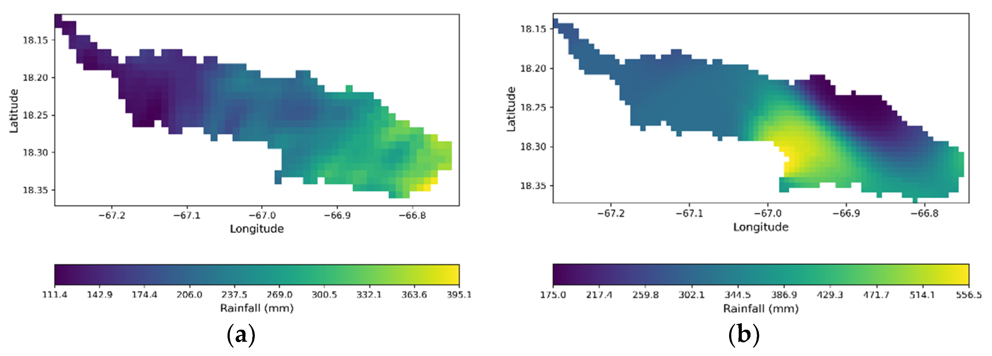
Figure 6a shows the cumulative rainfall from the simulated Hurricane María using the WRF model. In addition, 63 different rain gauges from the National Weather Service (NWS), which reported the cumulative rainfall for 48 h, were used to generate a rainfall distribution map using the inverse distance weighted (IDW) interpolation method with a spatial resolution of 700 m. Subsequently, this map was cropped to show the cumulative rainfall for the Añasco watershed, as shown in Figure 6b. A comparison made between these two cumulative maps indicates a difference in the volume of 65 million cubic meters, which translates to an error of approximately 35 % (Table 3).
Figure 7 shows WRF precipitation rainfall, NWS cumulative rainfall, and the error in percentages between the WRF and NWS cumulative rainfall. A correction of the WRF time series was performed using the cumulative WRF rainfall and the NWS interpolated rainfall for the whole of PR; for this correction, it was assumed that the temporal distribution of the rainfall in the WRF model was correct. Therefore, the only variable to modify was the spatial distribution of the rainfall. To correct rainfall, Equation (7) was used to compute the distributed error between the two cumulative maps with respect to the WRF cumulative rainfall. Subsequently, Equation (8) was implemented to adjust the original hourly WRF precipitation values using the distributed errors previously described to obtain the corrected hourly WRF precipitation.
ε i , j = ( R i , j W R F R i , j N W S ) R i , j W R F  
R i , j c o r r e c t ( t ) = R i , j W R F ( t ) + R i , j W R F ( t ) ε i , j  
where, ε i , j is the distributed error between the two cumulative maps in position ith, jth, R i , j W R F is the WRF cumulative rainfall, R i , j N W S is the NWS cumulative rainfall, R i , j W R F ( t ) is the hour WRF rainfall at t time, and R i , j c o r r e c t ( t ) is the hour corrected rainfall at t time.
Three optional hydrographs were considered to recreate the flooding event during Hurricane María:
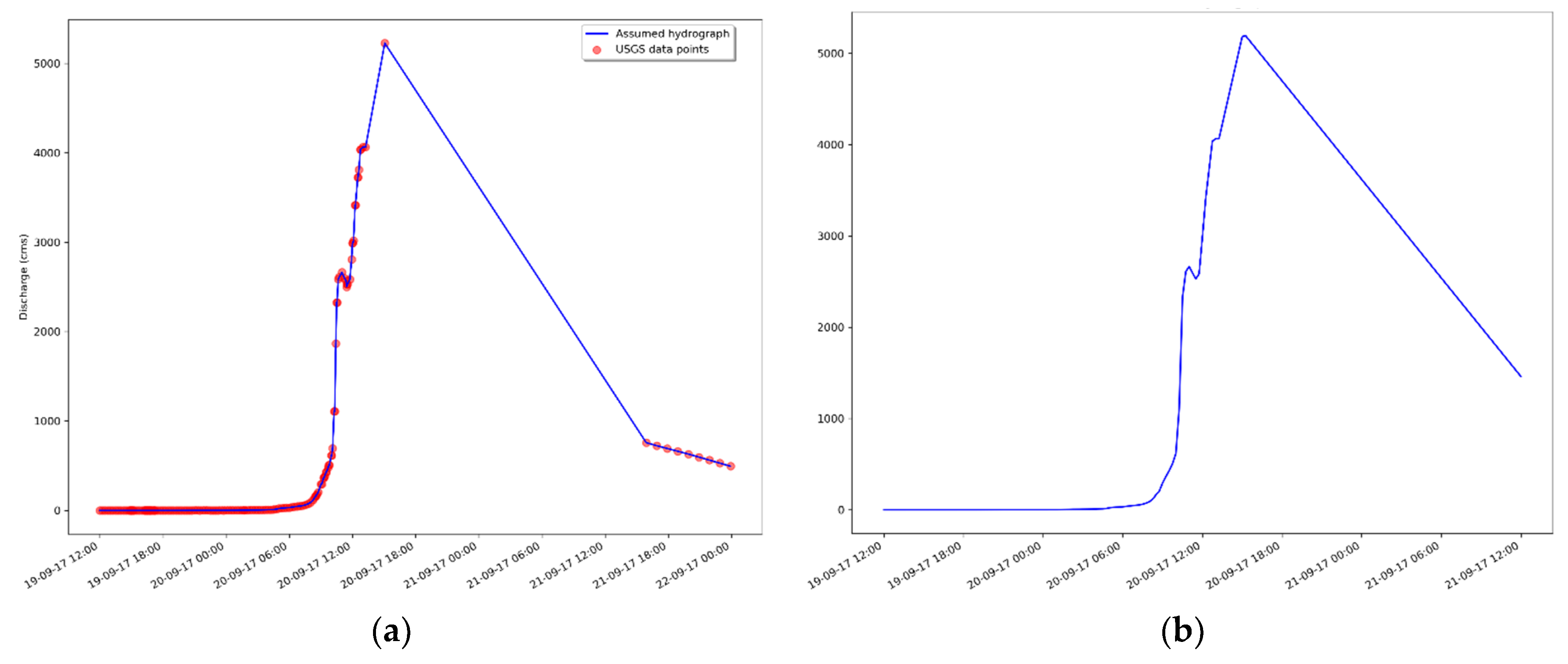
  • During Hurricane María, the USGS stream discharge gauge stopped working when it reported a maximum discharge measurement of almost 5200 m3 s−1, assumed to be the peak discharge for the whole event. Consequently, there is a gap of nearly 24 h where there is no data available, and after that, the USGS reported an estimated discharge. A simple linear regression was employed to interpolate the data to fill the gap and obtain time series values every 15 min. Figure 8a shows the final built hydrograph superimposed on the USGS discharge data. The time series, limited to 48 h (Figure 8b), was used to simulate the inflow boundary condition at the upstream location in Sub-watershed 1 for two scenarios (defined below).
  • The calibrated parameters obtained in the calibration process were used for Hurricane María to obtain the output hydrograph for Sub-watershed 2 using the WRF rainfall and the corrected rainfall separately. Following this, each output hydrograph obtained was used as an inflow hydrograph at the upstream location for Sub-watershed 1 to reproduce the flooding event during Hurricane María.

3.2.2. Storm Surge

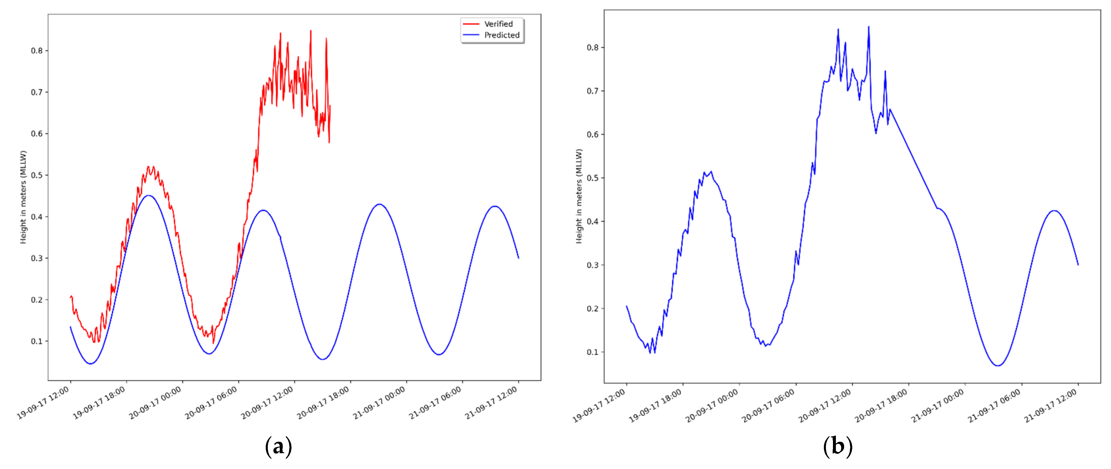
According to the Hurricane María report developed by NOAA, the storm surge in Western PR reached values between 1 and 3 feet (0.3 and 0.9 m) [60]. A NOAA tide station (9759394) was identified close to the coast of the Añasco watershed, which contained data from predicted and partially observed water height levels during Hurricane María. It was noticed that the maximum height of the water level (using the Mean Lower Low Water, MLLW) was approximately 0.85 m. Subsequently, it was decided to merge the predicted and the observed data to obtain a height water level variation over time. The last point of the observed data was merged with the closest predicted water level height to create a smooth curve, as shown in Figure 9.

3.2.3. Hydrologic Modelling Approaches (HMAs)

Six different approaches were created to evaluate and analyze the flooding results in the lower area of the Añasco watershed (Table 4).

3.2.4. Flood Depth Validation

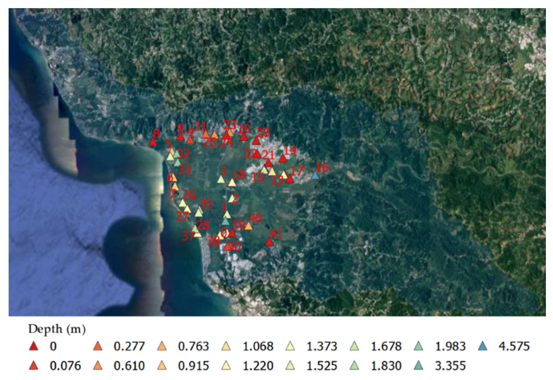
To validate the results from the flooding model, a survey was carried out to obtain an estimate of the flooding depth from the residents around the area affected during the Hurricane María. It should be mentioned that the flooding extent could not be obtained due to the lack of satellite images during the event. Several trips were made to the study area to interview people to obtain information about their experience during Hurricane María. People were asked, based on their recollection, how high the floodwater rose. Typically, they would point to a position on a wall or indicate the depth relative to a part of their body, for example, their knee or their waist. Table A4 gives the survey results, including the latitude and longitude of the interview location and the depth of flooding. In the results section of this paper, the simulated flooding will be compared to the depths obtained from the face-to-face interviews provided in Table A4; the geolocation and the distribution of the data collected can be observed in Figure 10. A python script was created to transform the coordinate reference system from WGS 84 (ESPS:4326) to the same coordinate reference system used in the GSSHA output flooding map, WGS 84/UTM zone 19N. Subsequently, the same python script was used to obtain the flooding depth at each of the survey locations in the output flooding map from GSSHA, in order to compare the results.

3.2.5. Methodology for Assessing Impacts to Critical Infrastructure

A python script was written to identify the infrastructure affected by the flooding. Input to the script included shapefiles with the geolocated infrastructure and each of the flooding maps. In this study, we assumed that a flood depth greater than 20 cm was defined as the criteria of failure for each of the water, electrical and public infrastructures. Table 5 summarizes all the infrastructures that were considered and their quantity within the study area.

4. Results

4.1. Calibration Results

As was mentioned previously, two methods available in GSSHA were used to calibrate the model. The SLM calibration method took almost 72 h to finish compared to the MLSL method, which took more than 147 h. The final calibrated parameters are summarized in Table 6.
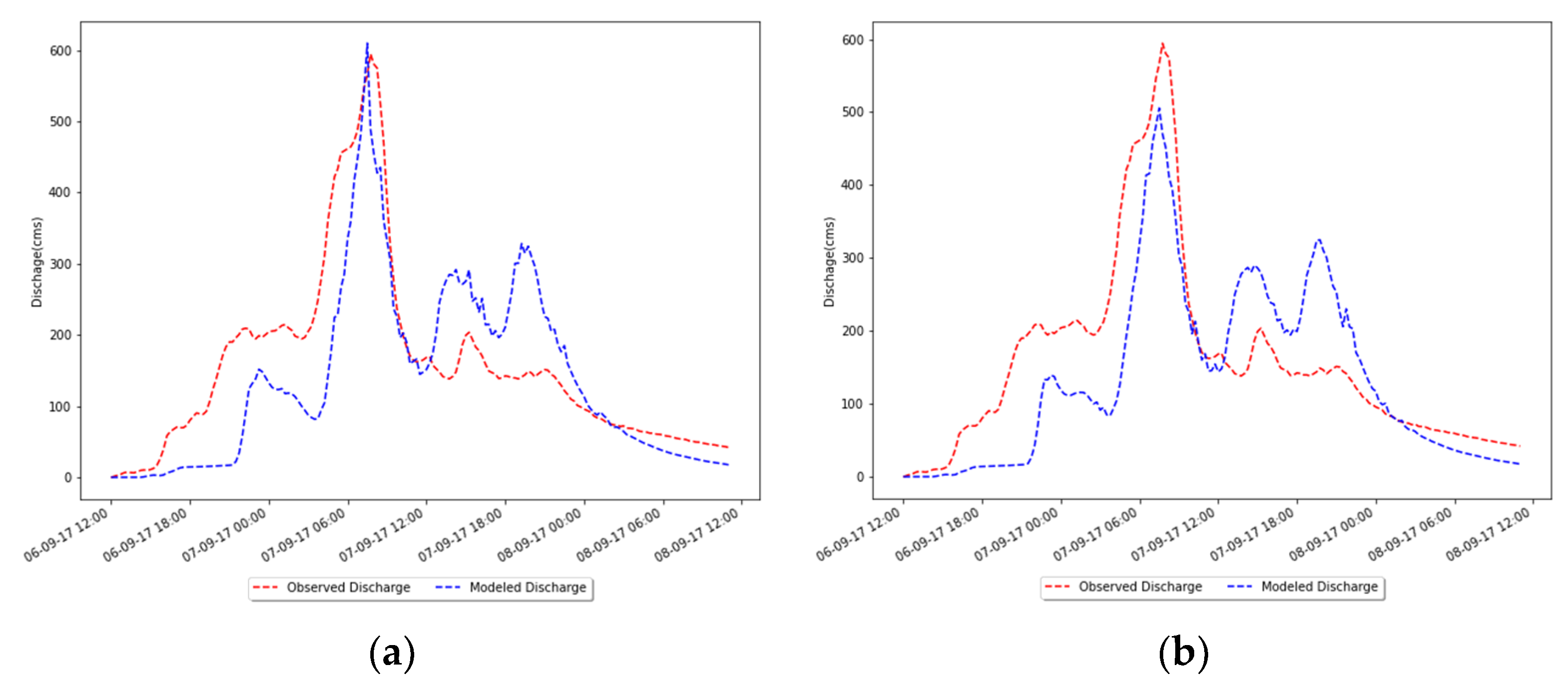
Having output hydrographs for each of the calibrations and the observed hydrograph, GSSHA computed the performance evaluation criteria to indicate which models had the better results. As shown in Table 7, the SLM calibration method achieved all the evaluation criteria to be satisfactory. Unfortunately, the MLSL calibration method did not achieve two of the evaluation criteria. Therefore, the parameters obtained in the SLM calibration method were utilized to validate the 2007 rainfall event.
Figure 11a,b shows the comparison of the observed and modeled hydrograph during Hurricane Irma using the calibrated parameters from the SLM calibration method and the MLSL calibration method, respectively. Additionally, it can be observed from Table 7 that the PBIAS values are positive, which mean that the modeled hydrograph underestimates the amount of volume below the hydrograph.

4.2. Validation Results

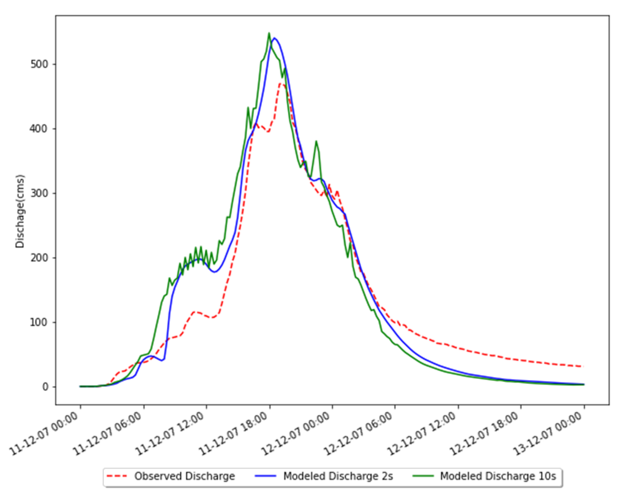
In this section, the calibrated parameters obtained using the SLM calibration method were validated using a rainfall event from 11–13 December 2007. In this case, two simulations were made (Figure 12), using a time step of 2 s and a time step of 10 s. The 10 s time step was used first; however, there was a region in the hydrograph where an oscillation in the discharge occurred. For this reason, it was decided to decrease the time step to 2 s, and as a result, the oscillatory behavior was eliminated. In Table 8, it can be seen that all the evaluation criteria are satisfied, and the evaluation metrics improved when a time step of 2 s was employed. Moreover, it was evidenced how the computational time increased when a time step of 2 s was used compared to a time step of 10 s, from a 3.6 h runtime (time step of 10 s) to a 16 h runtime (time step of 2 s). In addition, it should be noted from the PBIAS value in Table 8 that the validation results produced an overestimation in comparison to the measured discharge.
In addition to the validation results, the calibrated model was used with the Hurricane María WRF rainfall (with and without correction) to obtain the hydrographs at the USGS stream discharge gauge location. These hydrographs were used in the next section to reproduce the flooding in the coastal flood plain. The hydrograph 1 and hydrograph 2 in Figure 13 show the output hydrographs obtained using the WRF rainfall and the corrected rainfall over Sub-watershed 2.

4.3. Flooding Results

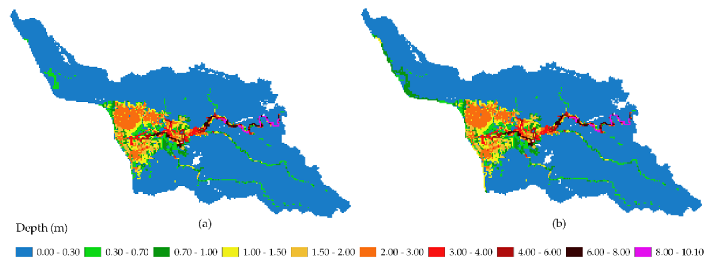
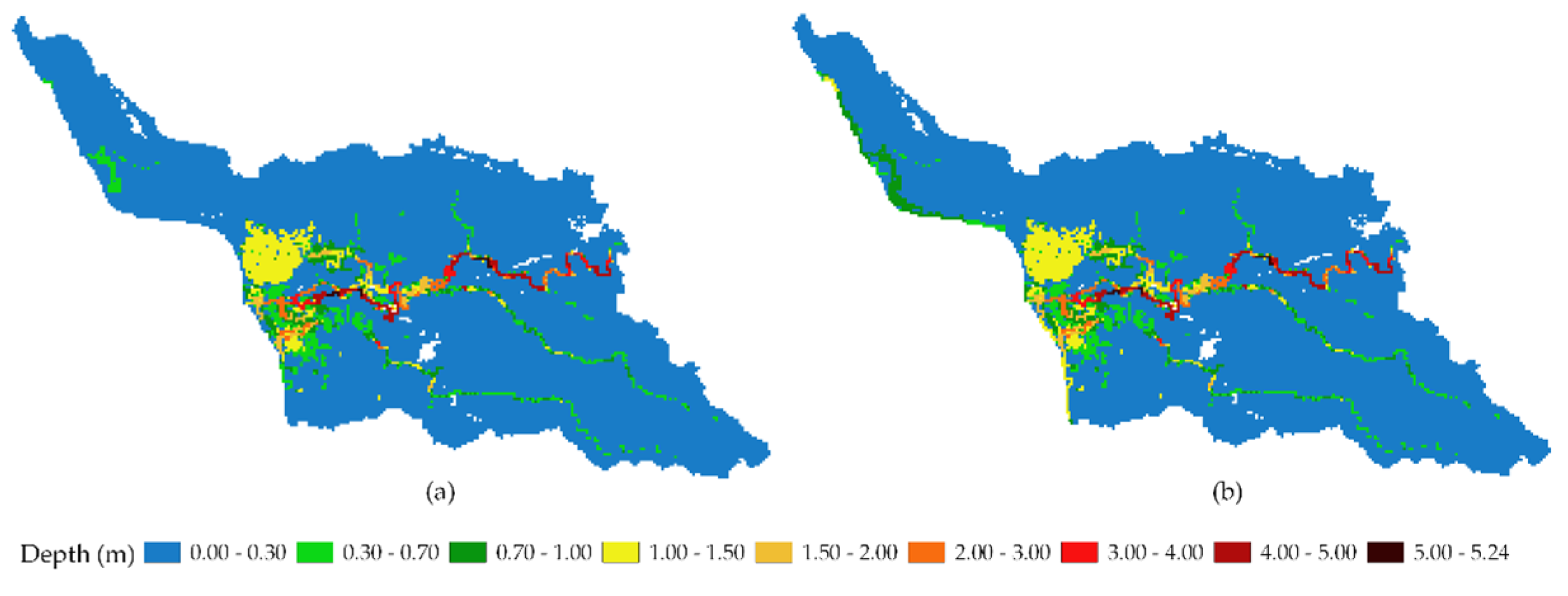
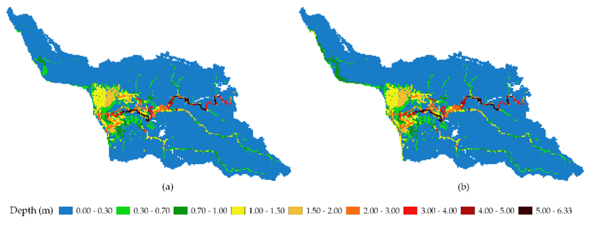
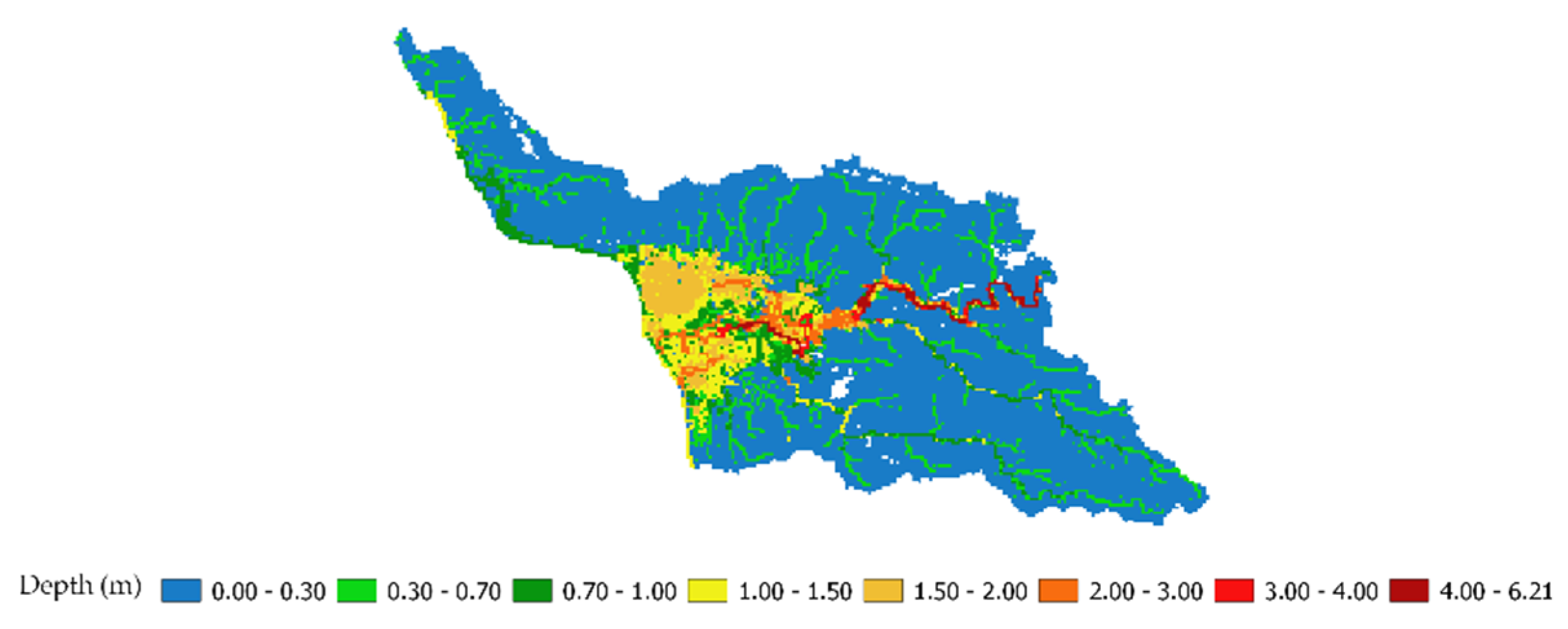
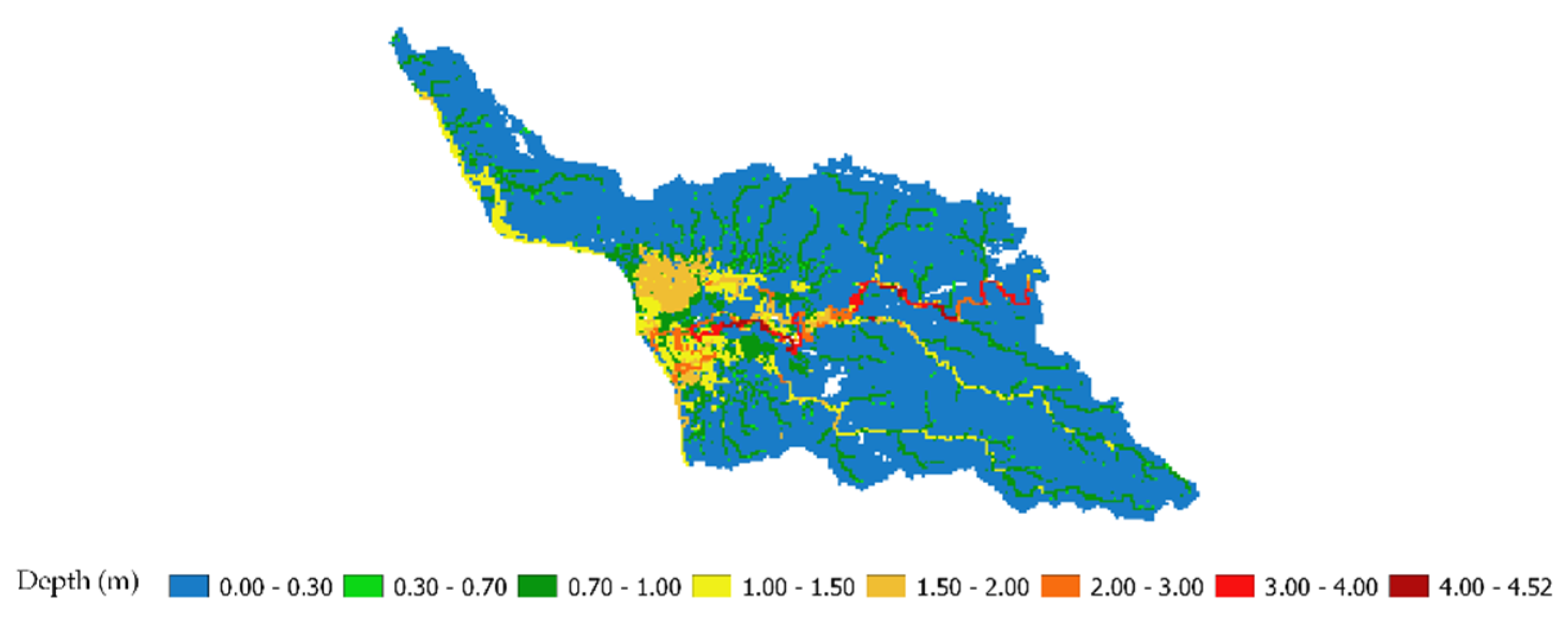
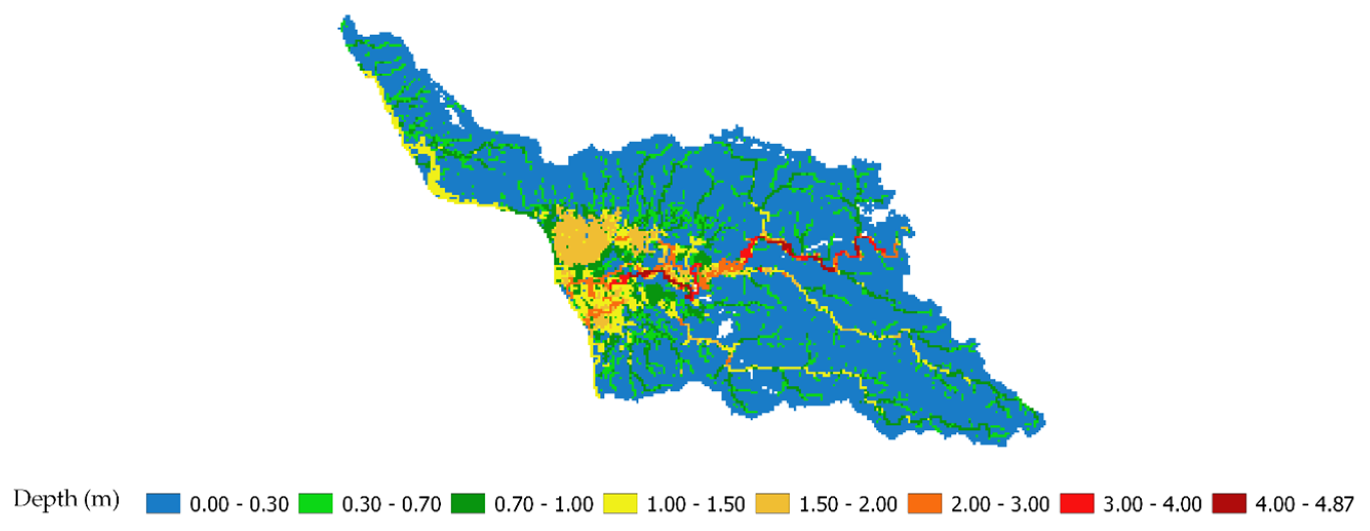
HMA 1 and 2 in Figure 14 show how the significant amount of discharge reported by the USGS stream discharge station affected the lower area of the Añasco watershed, especially along the coastal zone. The model produced a large extent and depth compared to the other HMAs (Figure 15 and Figure 16). It should be noted that the incorporation of the storm surge in HMAs 2, 4, and 6 produced less than 1 m of flooding in the areas close to Añasco Bay. However, incorporating the storm surge did not produce considerable changes in the central part of Sub-watershed 1, where much of the flooding occurred. On the other hand, it can be noted in Figure 16 how the bias corrections are noticeable in the flooding map, producing a more significant extent of flooding than the HMAs of Figure 15, which represent the original result of WRF without any correction.

4.3.1. Flood Validation Using Survey Data

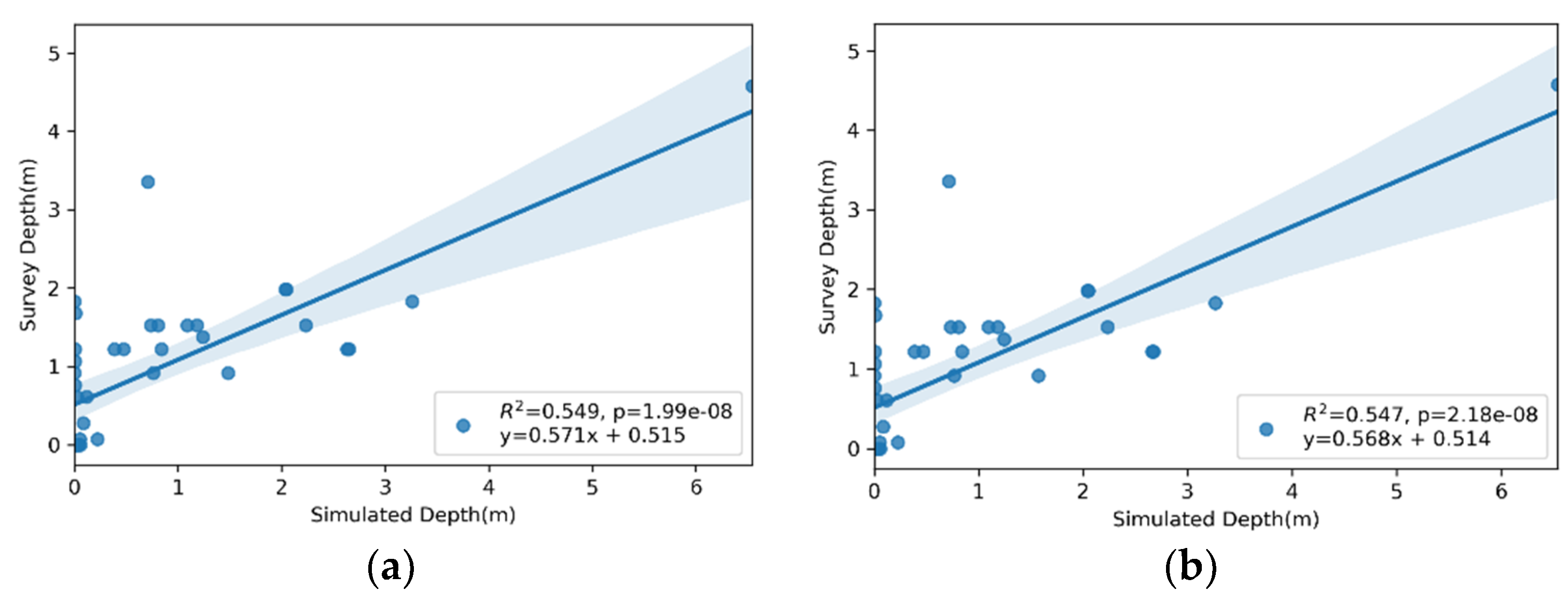
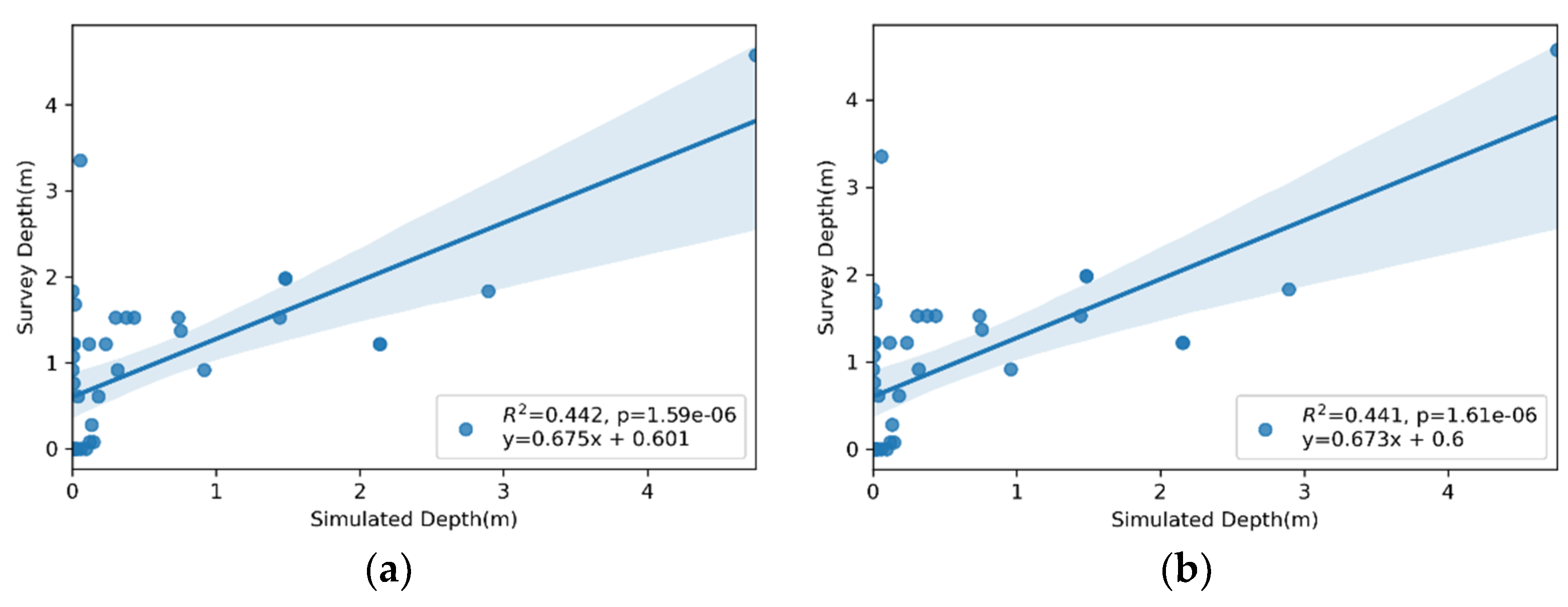
This section presents the comparison between the flood depths obtained from the face-to-face interviews with the model-simulated flood depths for the six HMAs (Figure 17, Figure 18 and Figure 19). It is noted that there were no noticeable differences between the simulations with and without storm surge. For example, HMAs 1 and 2 (Figure 17a,b) simulated identical conditions, the only difference being the storm surge in the HMA 2. In general, the simulated flood depths in HMAs 1 and 2 were larger than for the other HMAs. The linear regression equations and the R2 and p values are provided in each of the graphs with the 95% confidence interval. It should be noted in Figure 17, Figure 18 and Figure 19 how the p-values are less than the significance level (p-value ≤ 0.05), meaning that the data provide enough evidence to reject the null hypothesis, and that no correlation exists between the two datasets. The flood depth estimates can be improved by adjusting the flood depths using the linear regression equations. Figure 20, Figure 21 and Figure 22 show the flood depth maps for HMAs 2, 4, and 6, corrected using the flooding results from Figure 14b, Figure 15b and Figure 16b and the linear regression equation from Figure 17b, Figure 18b and Figure 19b to predict the survey depth values. The equation was used to predict flooding depth greater than 0.05 m, in order to avoid increases in depth when the flood depth was zero because of the intercept of the equation.

4.3.2. Extent of Flooded Area

The lack of satellite images, such as Synthetic Aperture Radar (SAR), made it impossible to obtain details of the flood extent during Hurricane María. Therefore, the area of the 500-year annual chance of flood hazard map from FEMA was used to compare the extent of flooding. Figure 23 shows the 500-year extent of flooding, which has an area of 34,789,370 m2.
Table 9 shows the flooded area for each HMA and the percentage differences from the FEMA 500-year flood area (Figure 23). The predicted flooded areas from all HMAs were less than FEMA’s 500-year flood area. The lowest percentage difference was for HMA 2 corrected (−13.51%). In addition, the HMAs 5 and 6, where rainfall bias corrections were applied, had smaller differences compared to the results using the original WRF rainfall data (HMAs 3 and 4). We compared the areas from the different HMAs with the 500-year annual chance of flood hazard map, assuming that the character of Hurricane María corresponded to this kind of event and taking into account that it is the maximum return period available from FEMA.

4.4. Critical Infrastructure

In this section, different water, electrical, and public infrastructure locations were used to evaluate the flooding impacts, assuming infrastructure failure when the flood depth is greater than 20 cm. In this analysis the simulated flood depths were corrected using the regression equations presented in Figure 17b, Figure 18b and Figure 19b. Although the regression analyses did not result in R2 values close to 1, the application of the regression equations will significantly improve the flood depth estimation.
Table 10 and Table 11 show the number of water and public/electrical infrastructures impacted by flooding, respectively. In Table 10, it is evident how some of the potable and sewer water components are potentially affected by the flooding caused by Hurricane María; specifically, sewer pump stations, potable water pump stations, and some of the wells owned and managed by the water authority (Autoridad de Acueductos y Alcantarillado de PR [AAA]). Additionally, it can be shown in Table 10 that most of the sewer pump stations are affected by flooding in HMAs 2 and 6. On the other hand, four potable water pump locations were impacted by the flooding event during Hurricane María in all the HMAs. Furthermore, some wells not located in the flood-prone areas were affected by HMAs 5 and 6. The flooding depth increased in some other areas due to the increment of the bias-corrected WRF rainfall. These failures are critical, especially the potable water components because they cause the disruption of potable water in the system. For example, pump stations are needed to fill water in the system tanks, deliver water to higher location customers, or increase the flow rate to achieve customer requirements.
A flood analysis of some other public and electrical infrastructure was conducted (Table 11). From the evaluation, we determined that there were no electrical substations or transmission centers affected by the flooding event during Hurricane María for any of the HMAs. On the other hand, Table 11 shows a public school was affected by Hurricane María flooding, occurring in four of the six HMAs.
Table 12 and Table 13 show the number of water and public/electrical infrastructures impacted, respectively, using the linear regression approximation for flooding. With the corrected flooding, it is noted (Table 12) how the quantity of affected infrastructure increases, especially the sewer and potable pump stations in HMA 2 (relative to Table 10); additionally, a number of wells were impacted. On the other hand, electrical infrastructure shows no damage in the transmission center and substations (Table 13), while the number of public schools affected by flooding increased.

5. Discussion

Based on the evaluation criteria, the validation results can be considered very good, with R2 = 0.946, NSE = 0.903, PBIAS (%) = −1.87, and volume error = 1.9%. The model was able to successfully capture 95% of the variation in the streamflow variability. On the other hand, the calibration results were not as good, indicating that the model could only capture 61% of the variation in the streamflow variability and have a 15.2% error in the volume estimate. Only one other study calibrated hourly stream discharge for the Añasco River. Using the Vflo model, [27] adjusted model parameters for eight different storms. The storms that were evaluated were significantly smaller than the storms we considered in this study. Although they did not use the same evaluation metrics that we used, their model performance appears to be comparable. All other hydrologic model studies for the Añasco watershed simulated daily or monthly average discharge. The authors of [26,28,29] reported coefficients of determination (R2) of 0.24, 0.50, and 0.57, respectively. The authors of [28] did not perform a formal model calibration but rather compared their model, configured with best-estimated model parameters, with available stream gauge data. Although reporting on a model calibration, [25] did not provide calibration statistics.
There are various sources of uncertainty that may explain the lower metrics for Hurricane Irma calibration, including:
  • The rating curve used by the USGS to convert river stage to discharge may not have been accurate during the Hurricane Irma event.
  • Although an effort was made to accurately account for the water released from the lakes in the upper Añasco watershed, the PR Energy and Power Authority (PREPA), the agency that manages the lakes, could not provide any information on discharges from the lakes.
  • NEXRAD radar rainfall data may also introduce errors into the hydrologic simulation. Rojas Gonzalez [26] reported a simulation of streamflow for the Añasco River in which NEXRAD significantly overestimated the rainfall. A known problem associated with radar rainfall in Western PR is related to the radar’s inability to see low clouds (less than 3000 m) at large distances from the radar facility due to the earth’s curvature [27]. This problem would be expected to produce underestimates in rainfall. However, one of the authors of this paper has considerable experience using radar rainfall in Western PR and has observed both under and overestimation compared with NWS rain gauges.
Time series rainfall from rain gauges was not available for Hurricane María. Consequently, it was necessary to use a WRF model rainfall dataset. In general, the WRF model of [61] did a good job of simulating rainfall over PR, with a Normalized Root Mean Square Error (RMSE) of 0.2. However, we observed inconsistencies in the total rainfall depths within our study area compared with the NWS interpolated rain gauge data. A correction of the WRF time series rainfall was made using the NWS rain gauge data. There was little observable difference in flooding between the corrected and noncorrected rainfall (Figure 15 and Figure 16).
Neither the WRF nor the bias-corrected WRF rainfall datasets could produce the large volume measured by the stream gauge during Hurricane María (Figure 8), and the use of the USGS stream gauge data for the inflow boundary condition to Sub-watershed 1 resulted in significantly greater flooding (Figure 14) than resulted from the WRF noncorrected rainfall (Figure 15) or the corrected rainfall (Figure 16).
The authors of [28] simulated the combined effect of storm surge and overland runoff in Eastern PR for Hurricane George. Although the peak of the storm surge, estimated to be 3 m, did not correspond with the peak runoff, the compound effect did aggravate flooding. In this study, we also used GSSHA to simulate the combined effects of storm surge and runoff. The authors of [60] estimated the storm surge in the study area to be 0.3 to 1 m. Figure 14, Figure 15 and Figure 16 show flooding within and without storm surge included. The figures indicate that the impact from the storm surge was minimal. However, it should be noted that individuals interviewed in the study living near the coast observed the storm surge.
Figure 17, Figure 18 and Figure 19 show the Hurricane María flood depths obtained from face-to-face surveys versus the simulated flood depths for the six simulated HMAs. The data pairs associated with data points Nos. 17 and 32 were considered outliers and removed from the dataset. Datapoint No. 17 was removed because there was another data point within the same model grid pixel (No. 18) with an observed depth three times that of No. 17. There was considerable small-scale topographic variation, which the model could not capture with the 100 m grid spacing. Datapoint No. 32 was located at a car dealership. The grid pixel contained two large buildings with roof heights of approximately 10 m and a raised highway approximately 5 m above the car dealership parking lot. The complexity of the topography at the location may have introduced an error in the grid elevation. It should also be noted that the survey data was acquired from resident interviews and not through post-flooding analysis which introduces some uncertainties in the surveyed depth; additionally, the flooding extent could not be validated because of the lack of satellite images during the Hurricane María event.
In general, the GSSHA model did not provide highly accurate flood depths, as evidenced from the low coefficients of determination (R2) values of 0.547, 0.399, and 0.441 for HMAs 1 and 2, 3 and 4, and 5 and 6, respectively (note that the r2 values were the same with or without storm surge due to the negligible effect storm surge had on flooding at the locations of the comparisons). To improve the model’s ability to estimate flood depths, the linear regression equations were applied to enhance the depth estimates. Finally, a GIS intersection analysis was performed to evaluate infrastructure impacts, assuming to occur for flood depths greater than 20 cm. The analysis revealed numerous water components that were potentially impacted. No electrical infrastructure was identified as being impacted, while several public schools were potentially impacted. Electric infrastructure is known to have been damaged in the study area during Hurricane María; however, the cause is likely attributable to wind damage.

5.1. Model Limitations

Some of the limitations of the model are described:
  • The model used in this study was developed for large storm events proceeded by saturated soil conditions. Consequently, the model has not been calibrated for conditions when soil saturation is low and infiltration becomes a significant factor. Future efforts should consider calibrating the average matric suction at the wetting front during periods of low soil saturation.
  • The hydrologic model of Sub-watershed 1 was not calibrated in this study. However, the depths and extent of the flood were compared with data obtained from a homeowner survey. Although the analysis did not yield a high correlation between the observed and simulated flood depths, we applied the resulting regression equations, which significantly improved the performance of the flood depth estimation. The flood depths obtained from the face-to-face interviews were limited to flood plain areas where people were present during Hurricane María.
  • The model was based on a simplified conceptualization of the land surface parameters. Single values of roughness and hydraulic conductivity were used for the dominant land use/soil in Sub-watershed 2. More accurate distribution of these parameters in the watershed may help to improve the model calibrations.

5.2. Future Work

Recommendations for future research include:
  • Couple the flood model with a WRF rainfall forecast model to obtain 2- to 3-day advanced flooding warnings.
  • Couple the flood modelling results with a Power/Water network model.
  • Expand the model domain to include the Culebrinas, Yagüez, and Guanajibo watersheds. This will expand the area of coverage from 350 km2 to over 900 km2.
  • Continue to work with the water and electric authorities to refine our approach for identifying impacted infrastructure.
  • Use the model to investigate ways to mitigate flooding in Sub-watershed 1. For example, evaluate changes in agricultural land-use practices or incorporate natural infrastructure.

6. Conclusions

A GSSHA model was developed in this study to simulate overland runoff, streamflow, and coastal storm surge in Western PR during Hurricane María. The upper gauged watershed (Sub-watershed 2) was calibrated with stream discharge data for Hurricane Irma and validated using a comparable storm from 11–13 December 2007. The Secant Levenberg–Marquardt (SLM) method was used for model calibration. Because the NEXRAD radar was damaged during the hurricane, we used the rainfall generated from the WRF model. Additionally, a bias-corrected WRF rainfall data set was used. The bias corrections were derived from the NWS total rainfall dataset. Flooding was simulated in the coastal flood plain (Sub-watershed 1) for six different HMAs. Storm surge did not appear to aggravate the flooding, at least in the areas considered in this study. Although the simulated flooding depth did not correspond exactly with the observed data, a set of calibration equations was employed to improve the model’s performance. An analysis was conducted to determine the impact of flooding on water, electricity, and public infrastructure. Numerous water infrastructure components were impacted, including sewer pump stations, potable water pump stations, and wells. No electrical infrastructure sustained damage from flooding (per our criteria: water depth > 20 cm), while several public schools were damaged by flooding. Future research will focus on expanding the model domain and coupling the flood model with a rainfall prediction model to produce a flood forecast alarm tool.

Author Contributions

Conceptualization, S.A.M.M. and E.W.H.; methodology, S.A.M.M. and E.W.H.; software, S.A.M.M.; validation, S.A.M.M.; formal analysis, S.A.M.M. and E.W.H.; investigation, S.A.M.M., E.W.H., R.M.K. and J.E.G.; collection of survey data, E.W.H.; resources, J.E.G. and E.W.H.; data curation, J.E.G.; writing—original draft preparation, S.A.M.M. and E.W.H.; writing—review and editing, E.W.H., R.M.K. and J.E.G.; visualization, S.A.M.M.; supervision, E.W.H., R.M.K. and J.E.G.; project administration, J.E.G. and E.W.H.; funding acquisition, J.E.G. and E.W.H. All authors have read and agreed to the published version of the manuscript.

Funding

Financial support was provided by the National Science Foundation (NSF) (grants 0313747 & 1832576). Findings, opinions, or conclusions expressed in this paper do not necessarily reflect those of the NSF.

Institutional Review Board Statement

Not applicable.

Informed Consent Statement

Not applicable.

Data Availability Statement

Data are available upon request from the corresponding author.

Acknowledgments

We would like to thank Michael Piasecki for the use of the GSSHA software license used during the study. We are indebted to the Autoridad de Acueductos y Alcantarillados (AAA) and to Joel Lugo, Director of the Western Region, for sharing data and information; and also Engineer María Torres. Thanks to Alicia Tyson for processing the SSURGO soil data and Elías Cheveré Vázquez for data collection and Python programming.

Conflicts of Interest

The authors declare no conflict of interest. Reference to any proprietary software, equipment, merchandise, or brand name in no way implies an endorsement of the software, equipment, merchandise, or brand name.

Appendix A

Table A1. Percentage distribution of the land classes within Sub-watershed 1 and Sub-watershed 2 from Figure 2, and the Manning’s values for each of the classes [67].
Land ClassSub-Watershed 1 (%)Sub-Watershed 2 (%)Manning’s Values
Mixed Forest77.559.10.1
Cultivated7.92.90.037
Low Intensity Developed4.78.40.05
Scrub/Shrub3.67.90.05
Palustrine Forested Wetland3.00.50.1
Medium Intensity Developed1.04.60.1
Grassland0.92.70.034
Water0.60.60.02
Pasture/Hay0.45.00.033
High Intensity Developed0.32.80.13
Bare Land0.10.50.09
Developed Open Space0.11.00.02
Palustrine Scrub/Shrub Wetland0.00.40.048
Unconsolidated Shore0.00.10.04
Palustrine Emergent Wetland0.03.00.045
Estuarine Forested Wetland0.00.20.1
Estuarine Scrub/Shrub Wetland0.00.00.048
Estuarine Emergent Wetland0.00.10.045
Table A2. Percentage Distribution of soil classes within Sub-watershed 1 and Sub-watershed 2 from Figure 2.
Soil ClassSub-Watershed 1 (%)Sub-Watershed 2 (%)
clay77.566.8
clay loam16.916.8
loam0.53.0
loamy sand0.00.0
sand0.02.4
sandy loam0.00.0
silt clay loam1.610.8
silty clay3.10.0
silty loam0.40.2
Table A3. Values assumed for the Green Ampt infiltration method [70].
Infiltration VariablesClay LoamLoamy SandClaySilt Clay LoamSandy LoamLoamSilty ClaySilty LoamSand
Hydraulic conductivity (cm/h)0.25.980.060.22.181.320.10.6823.6
Capillary head (cm)20.886.1331.627.311.018.8929.2216.684.95
Porosity (m3/m3)0.4640.4370.480.4710.4530.460.4790.5010.44
Pore Distribution Index (cm/cm)0.2420.5530.170.1770.3780.250.150.2340.69
Residual Saturation (m3/m3)0.0750.0350.090.040.0410.030.0560.0150.02
Field Capacity (m3/m3)0.3180.1250.40.3660.2070.270.3870.330.09
Wilting Point (m3/m3)0.1970.0550.270.2080.0950.120.250.1330.03
Table A4. Locations and depths of flooding during Hurricane María obtained from residents in the Añasco flood plain (Sub-watershed 1).
No.LatLonDepth (m)Description
018.24994−67.16051.22Shell Station on Road 2
118.25932−67.16041.525West Power Company Road 2
218.26726−67.15761.525First Medical Cannabis
318.27699−67.16331.525Grooming Machine near Road 2
418.29674−67.17920.07625Horse Facility
518.2908−67.18890.915Bakery
618.27804−67.18830.915In street at HP beach home
718.27354−67.18740.915Close to small waterway north of Añasco River
818.29619−67.19870Gas Station
918.29853−67.18430Colmado
1018.28207−67.14050Añasco Plaza
1118.28054−67.13651.0675Auto Supply Store
1218.27885−67.130Hardware Store
1318.27883−67.13051.22Back yard of home next to hardware store
1418.2871−67.13080Urbanization on north side of Añasco
1518.28142−67.14071.6775Daycare Center behind Municipal Building
1618.27843−67.1144.575Residential home
1718.27674−67.12730Residential home
1818.27534−67.15751.22Roadside Store
1918.2981−67.15130Pharmacy Road 402
2018.29606−67.14470Urbanization
2118.28486−67.13840Urbanization
2218.28942−67.14430Industrial Park
2318.30017−67.15850.61Oil Change Garage
2418.29886−67.16030Laundry Mat
2518.29912−67.16650.61Road 402 in front of Coffee Shop
2618.26535−67.18351.22Urbanization close to Añasco River
2718.26223−67.18111.22Urbanization close to Añasco River
2818.25013−67.17581.22Grocery Store on Road 341
2918.256−67.16123.355Mazda Dealership on Road 2
3018.24323−67.16020.07625Church’s Chicken on Road 2
3118.2995−67.17110.27755House on Hwy 115
3218.28975−67.18631.9825No description
3318.28551−67.18591.9825No description
3418.28853−67.18971.525No description
3518.26178−67.17481.83No description
3618.2603−67.17521.525No description
3718.25227−67.17721.83No description
3818.24886−67.16421.3725No description
3918.25006−67.15780No description
4018.2535−67.14920.7625No description
4118.24555−67.13840No description

References

  1. Tanaka, K.; Fujihara, Y.; Hoshikawa, K.; Fujii, H. Development of a flood water level estimation method using satellite images and a digital elevation model for the Mekong floodplain. Hydrol. Sci. J. 2019, 64, 241–253. [Google Scholar] [CrossRef] [Green Version]
  2. Harmsen, E.W.; Goyal, M.R. Flood Assessment: Modeling and Parameterization; Apple Academic Press: Cambridge, MA, USA, 2018. [Google Scholar]
  3. Wu, H.; Adler, R.F.; Tian, Y.; Huffman, G.J.; Li, H.; Wang, J. Real-time global flood estimation using satellite-based precipitation and a coupled land surface and routing model. Water Resour. Res. 2014, 50, 2693–2717. [Google Scholar] [CrossRef] [Green Version]
  4. Ramos-Scharrón, C.; Garnett, C.; Arima, E. A Catalogue of Tropical Cyclone Induced Instantaneous Peak Flows Recorded in Puerto Rico and a Comparison with the World’s Maxima. Hydrology 2021, 8, 84. [Google Scholar] [CrossRef]
  5. Nicholls, R.; Zanuttigh, B.; Vanderlinden, J.P.; Weisse, R.; Silva, R.; Hanson, S.; Narayan, S.; Hoggart, S.; Thompson, R.C.; de Vries, W.; et al. Developing a Holistic Approach to Assessing and Managing Coastal Flood Risk. In Coastal Risk Management in a Changing Climate; Elsevier: Amsterdam, The Netherlands, 2015; pp. 9–53. [Google Scholar]
  6. U.S. DHS Science and Technology Critical Infrastructure. DHS. Available online: https://www.dhs.gov/science-and-technology/critical-infrastructure (accessed on 27 May 2021).
  7. Dept. for Transportation Great Britain. Transport Resilience Review: A Review of the Resilience of the Transport Network to Extreme Weather Events; Dept. for Transportation Great Britain: London, UK, 2014. [Google Scholar]
  8. AECOM. Natural Infrastructure—Coastal Resources, Freshwater & Forestry Briefing Document; Resilient Puerto Rico-Advisory Commision: San Juan, Puerto Rico, 2018. [Google Scholar]
  9. NOAA. NOAA Digital Coast, Office of Coastal Managment, Natural Infrastructure Resources. Available online: https://coast.noaa.gov/data/digitalcoast/pdf/natural-infrastructure.pdf (accessed on 30 May 2021).
  10. Pant, R.; Thacker, S.; Hall, J.W.; Alderson, D.; Barr, S. Critical infrastructure impact assessment due to flood exposure. J. Flood Risk Manag. 2018, 11, 22–33. [Google Scholar] [CrossRef]
  11. Dano, U.L. Flash Flood Impact Assessment in Jeddah City: An Analytic Hierarchy Process Approach. Hydrology 2020, 7, 10. [Google Scholar] [CrossRef] [Green Version]
  12. Lu, Q.-C.; Peng, Z.-R.; Zhang, J. Identification and Prioritization of Critical Transportation Infrastructure: Case Study of Coastal Flooding. J. Transp. Eng. 2015, 141, 04014082. [Google Scholar] [CrossRef]
  13. Chisolm, E.I.; Matthews, J.C. Impact of Hurricanes and Flooding on Buried Infrastructure. Leadersh. Manag. Eng. 2012, 12, 151–156. [Google Scholar] [CrossRef]
  14. Unterberger, C. How Flood Damages to Public Infrastructure Affect Municipal Budget Indicators. Econ. Disasters Clim. Chang. 2017, 2, 5–20. [Google Scholar] [CrossRef] [Green Version]
  15. Murdock, H.J.; De Bruijn, K.M.; Gersonius, B. Assessment of Critical Infrastructure Resilience to Flooding Using a Response Curve Approach. Sustainability 2018, 10, 3470. [Google Scholar] [CrossRef]
  16. Sánchez, J.G.A.; Houmanfar, R.A.; Alavosius, M.P. A Descriptive Analysis of the Effects of Weather Disasters on Community Resilience. Behav. Soc. Issues 2019, 28, 298–315. [Google Scholar] [CrossRef]
  17. Pokhrel, R.; Ramírez-Beltran, N.D.; González, J.E. On the assessment of alternatives for building cooling load reductions for a tropical coastal city. Energy Build. 2019, 182, 131–143. [Google Scholar] [CrossRef]
  18. López, G.G. The Multiple Layers of Environmental Injustice in Contexts of (Un)natural Disasters: The Case of Puerto Rico Post-Hurricane Maria. Environ. Justice 2018, 11, 101–108. [Google Scholar] [CrossRef]
  19. Puerto Rico Emergency Management Bureau. Joint Operational Catastrophic Incident Plan; Puerto Rico Emergency Management Bureau: San Juan, Puerto Rico, 2019; Version 1.10; p. 244. [Google Scholar]
  20. Georgescu, M.; Broadbent, A.M.; Wang, M.; Krayenhoff, E.S.; Moustaoui, M. Precipitation response to climate change and urban development over the continental United States. Environ. Res. Lett. 2021, 16, 044001. [Google Scholar] [CrossRef]
  21. Glenn, E.; Comarazamy, D.; González, J.E.; Smith, T. Detection of recent regional sea surface temperature warming in the Caribbean and surrounding region. Geophys. Res. Lett. 2015, 42, 6785–6792. [Google Scholar] [CrossRef]
  22. Gould, W.A.; Diaz, E.L.; Álvarez-Berríos, N.L.; Aponte-González, F.; Archibald, W.; Bowden, J.H.; Carrubba, L.; Crespo, W.; Fain, S.J.; González, G.; et al. US Caribbean, in Impacts, Risks and Adaptation in the United States: 4th National Climate Assessment; Reidmiller, D., Avery, C.W., Easterling, D.R., Kunkel, K.E., Lewis, K.L.M., Maycock, T.K., Stewart, B.C., Eds.; US Global Change Research Program: Washington, DC, USA, 2018; Volume 2, pp. 809–871. [Google Scholar] [CrossRef]
  23. Jury, M. Resolution-Dependent Perspectives on Caribbean Hydro-Climate Change. Hydrology 2020, 7, 93. [Google Scholar] [CrossRef]
  24. Hunter, J. A simple technique for estimating an allowance for uncertain sea-level rise. Clim. Chang. 2012, 113, 239–252. [Google Scholar] [CrossRef]
  25. van der Sande, C.; De Jong, S.; de Roo, A. A segmentation and classification approach of IKONOS-2 imagery for land cover mapping to assist flood risk and flood damage assessment. Int. J. Appl. Earth Obs. Geoinf. 2003, 4, 217–229. [Google Scholar] [CrossRef]
  26. Grek, E.; Zhuravlev, S. Simulation of Rainfall-Induced Floods in Small Catchments (the Polomet’ River, North-West Russia) Using Rain Gauge and Radar Data. Hydrology 2020, 7, 92. [Google Scholar] [CrossRef]
  27. Moftakhari, H.R.; Salvadori, G.; AghaKouchak, A.; Sanders, B.; Matthew, R.A. Compounding effects of sea level rise and fluvial flooding. Proc. Natl. Acad. Sci. USA 2017, 114, 9785–9790. [Google Scholar] [CrossRef] [Green Version]
  28. Silva-Araya, W.F.; Santiago-Collazo, F.L.; Gonzalez-Lopez, J.; Maldonado-Maldonado, J. Dynamic Modeling of Surface Runoff and Storm Surge during Hurricane and Tropical Storm Events. Hydrology 2018, 5, 13. [Google Scholar] [CrossRef] [Green Version]
  29. McInnes, K.; Hubbert, G.D.; Abbs, D.J.; Oliver, S.E. A numerical modelling study of coastal flooding. Theor. Appl. Clim. 2002, 80, 217–233. [Google Scholar] [CrossRef]
  30. Nofal, O.M.; van de Lindt, J.W.; Do, T.Q. Multi-variate and single-variable flood fragility and loss approaches for buildings. Reliab. Eng. Syst. Saf. 2020, 202, 106971. [Google Scholar] [CrossRef]
  31. Santiago-Collazo, F.L.; Bilskie, M.V.; Hagen, S.C. A comprehensive review of compound inundation models in low-gradient coastal watersheds. Environ. Model. Softw. 2019, 119, 166–181. [Google Scholar] [CrossRef]
  32. Santiago-Collazo, F.; Silva Araya, W.; González-López, J.; Maldonado-Maldonado, J. Flooding Effects Combining Storm Surge and Surface Runoff during Hurricane Georges on the Eastern Coast of Puerto Rico. Available online: https://www.scipedia.com/public/Santiago-Collazo_et_al_2017a (accessed on 1 April 2021).
  33. Chen, W.-B.; Liu, W.-C. Assessment of storm surge inundation and potential hazard maps for the southern coast of Taiwan. Nat. Hazards 2016, 82, 591–616. [Google Scholar] [CrossRef]
  34. Bates, P.D.; Dawson, R.J.; Hall, J.W.; Horritt, M.S.; Nicholls, R.J.; Wicks, J.; Hassan, M.A.A.M. Simplified two-dimensional numerical modelling of coastal flooding and example applications. Coast. Eng. 2005, 52, 793–810. [Google Scholar] [CrossRef]
  35. Dietrich, J.; Zijlema, M.; Westerink, J.; Holthuijsen, L.; Dawson, C.; Luettich, R.; Jensen, R.; Smith, J.; Stelling, G.; Stone, G. Modeling hurricane waves and storm surge using integrally-coupled, scalable computations. Coast. Eng. 2011, 58, 45–65. [Google Scholar] [CrossRef]
  36. Bhaskaran, P.K.; Gayathri, R.; Murty, P.; Bonthu, S.; Sen, D. A numerical study of coastal inundation and its validation for Thane cyclone in the Bay of Bengal. Coast. Eng. 2014, 83, 108–118. [Google Scholar] [CrossRef]
  37. Graeme, D.H.; McInnes, K.L. A Storm Surge Inundation Model for Coastal Planning and Impact Studies. J. Coast. Res. 1999, 15, 168–185. [Google Scholar]
  38. Ikeuchi, H.; Hirabayashi, Y.; Yamazaki, D.; Muis, S.; Ward, P.J.; Winsemius, H.; Verlaan, M.; Kanae, S. Compound simulation of fluvial floods and storm surges in a global coupled river-coast flood model: Model development and its application to 2007 Cyclone Sidr in Bangladesh. J. Adv. Model. Earth Syst. 2017, 9, 1847–1862. [Google Scholar] [CrossRef]
  39. Nguyen, H.Q.; Degener, J.; Kappas, M. Flash Flood Prediction by Coupling KINEROS2 and HEC-RAS Models for Tropical Regions of Northern Vietnam. Hydrology 2015, 2, 242–265. [Google Scholar] [CrossRef] [Green Version]
  40. Kornilova, E.; Krylenko, I.; Rets, E.; Motovilov, Y.; Bogachenko, E.; Krylenko, I.; Petrakov, D. Modeling of Extreme Hydrological Events in the Baksan River Basin, the Central Caucasus, Russia. Hydrology 2021, 8, 24. [Google Scholar] [CrossRef]
  41. Jamrussri, S.; Toda, Y. Simulating past severe flood events to evaluate the effectiveness of nonstructural flood countermeasures in the upper Chao Phraya River Basin, Thailand. J. Hydrol. Reg. Stud. 2017, 10, 82–94. [Google Scholar] [CrossRef]
  42. Giovanni-Prieto, M. Development of a Regional Integrated Hydrologic Model for a Tropical Watershed. Ph.D. Thesis, University of Puerto Rico, Mayaguez Campus, Mayagüez, Puerto Rico, 2007. Available online: https://hdl.handle.net/20.500.11801/1764 (accessed on 15 May 2021).
  43. Rojas González, A.M. Flood Prediction Limitations in Small Watersheds with Mountainous Terrain and High Rainfall Variability; University of Puerto Rico-Mayaguez Campus: Mayagüez, Puerto Rico, 2012; Available online: https://hdl.handle.net/20.500.11801/1085 (accessed on 15 May 2021).
  44. Torres-Molina, L.E. Flood Alert System Using Rainfall Data in the Mayagüez Bay Basin, Western Puerto Rico. Ph.D. Theses, University of Puerto Rico, Mayaguez Campus, Mayagüez, Puerto Rico, 2014. Available online: https://hdl.handle.net/20.500.11801/1156 (accessed on 15 May 2021).
  45. Ramos Scharrón, C.E.; Gilbes, F.; Torres-Pulliza, D.; Rodríguez-Guzmán, V.; Aceituno, J. Application of the Soil and Water Assessment Tool (SWAT) to Estimate Discharge and Sediment Yields from the Río Grande de Añasco Watershed, Puerto Rico; Final Report to UPR-Sea Grant; Island Resources Foundation: St. Thomas, VA, USA, 2014; 71p. [Google Scholar]
  46. Nilawar, A.P.; Calderella, C.P.; Lakhankar, T.Y.; Waikar, M.L.; Munoz, J. Satellite Soil Moisture Validation Using Hydrological SWAT Model: A Case Study of Puerto Rico, USA. Hydrology 2017, 4, 45. [Google Scholar] [CrossRef] [Green Version]
  47. Vieux, B.E. Distributed Hydrologic Modeling Using GIS, 2nd ed.; Springer: Berlin/Heidelberg, Germany, 2004. [Google Scholar]
  48. Beven, K.J.; Binley, A. The future of distributed models: Model calibration and uncertainty prediction. Hydrol. Process. 1992, 6, 279–298. [Google Scholar] [CrossRef]
  49. Molina, L.S.T.; Harmsen, E.W.; Cruz-Pol, S. Flood alert system using rainfall forecast data in Western Puerto Rico. 2013 IEEE Int. Geosci. Remote Sens. Symp. IGARSS 2013, 574–577. [Google Scholar] [CrossRef]
  50. Sepúlveda, N.; Perez-Blair, F.; Delong, L.; Trujillo, D.L. Real-Time Rainfall-Runoff Model of the Carraizo-Reservoir Basin in Puerto Rico; US Geological Survey: Reston, VA, USA, 1996. [Google Scholar]
  51. Vieux, B.E.; Vieux, J.E. Evaluation of a Physics-Based Distributed Hydrologic Model for Coastal, Island and Inland Hydrologic Modeling. In Coastal Hydrology and Processes; Water Resources Publications: Highlands Ranch, CO, USA, 2006; pp. 453–464. [Google Scholar]
  52. Diaz-Ramirez, J.N.; Perez-Alegria, L.R.; McAnally, W.H. Hydrology and Sediment Modeling Using BASINS/HSPF in a Tropical Island Watershed. Trans. ASABE 2008, 51, 1555–1565. [Google Scholar] [CrossRef]
  53. Cohen, E.; Sun, G.L.; Zhang, P.; Caldwell, P.; Krieger, S. Quantifying the Role of Forested Lands in Providing Surface Drinking Water Supply for Puerto Rico; U.S. Department of Agriculture Forest Service: Newtown Square, PA, USA, 2017; p. 28. [Google Scholar]
  54. Zhang, L.; Sun, G.; Cohen, E.; McNulty, S.G.; Caldwell, P.V.; Krieger, S.; Christian, J.; Zhou, D.; Duan, K.; Cepero-Pérez, K.J. An Improved Water Budget for the El Yunque National Forest, Puerto Rico, as Determined by the Water Supply Stress Index Model. For. Sci. 2018, 64, 268–279. [Google Scholar] [CrossRef] [Green Version]
  55. Miller, P.W.; Kumar, A.; Mote, T.L.; Moraes, F.D.S.; Mishra, D. Persistent Hydrological Consequences of Hurricane Maria in Puerto Rico. Geophys. Res. Lett. 2019, 46, 1413–1422. [Google Scholar] [CrossRef] [Green Version]
  56. Harmsen, E.W.; Mecikalski, J.R.; Reventos, V.J.; Álvarez Pérez, E.; Uwakweh, S.S.; Adorno García, C. GOES-PRWEB: Development, Validation and Application. Hydrology 2021, in press. [Google Scholar]
  57. Delong, L.; Schoellhamer, D. Computer Program HYDRAUX: A Model for Simulating One- Dimensional, Unsteady, Open-Channel Flow; US Geological Survey: Washington, DC, USA, 1989. [Google Scholar]
  58. Smith, M.B.; Seo, D.-J.; Koren, V.I.; Reed, S.M.; Zhang, Z.; Duan, Q.; Moreda, F.; Cong, S. The distributed model intercomparison project (DMIP): Motivation and experiment design. J. Hydrol. 2004, 298, 4–26. [Google Scholar] [CrossRef]
  59. DNRA. Informe Sobre la Sequía 2014-16 en Puerto Rico, División Monitoreo del Plan de Aguas, San Juan, Puerto Rico; Departamento de Recursos Naturales y Ambientales de Puerto Rico: San Juan, Puerto Rico, 2016. Available online: http://drna.pr.gov/wp-content/uploads/2017/01/Informe-Sequia-2014-2016.compressed.pdf (accessed on 15 May 2021).
  60. Richard, J.; Pasch, A.B.P.; Berg, R. National Hurricane Center Tropical Cyclone Report Hurricane Maria (AL152017) 16–30 September 2017. NOAA NWS, 2019. Available online: https://www.nhc.noaa.gov/data/tcr/AL152017_Maria.pdf (accessed on 15 May 2021).
  61. Pokhrel, R.; del Cos, S.; Rincon, J.P.M.; Glenn, E.; González, J.E. Observation and modeling of Hurricane Maria for damage assessment. Weather. Clim. Extrem. 2021, 33, 100331. [Google Scholar] [CrossRef]
  62. Glenn, E.; Smith, T.; Gálvez, J.; Davison, M.; Hibbert, K.; González, J. Tropical Convection in the Caribbean and Surrounding Region during a Regional, Warming Sea-Surface Temperature Period, 1982–2020. Hydrology 2021, 8, 56. [Google Scholar] [CrossRef]
  63. Office for Coastal Management, 2021: 2010 C-CAP 30 Meter Land Cover of Puerto Rico from 2010-06-15 to 2010-08-15. NOAA National Centers for Environmental Information. Available online: https://www.fisheries.noaa.gov/inport/item/48300 (accessed on 30 May 2020).
  64. Web Soil Survey. Available online: http://websoilsurvey.nrcs.usda.gov (accessed on 21 February 2013).
  65. U.S. Army Corpes of Engineers. Gridded Surface Subsurface Hydrologic Analysis. Available online: https://www.erdc.usace.army.mil/Media/Fact-Sheets/Fact-Sheet-Article-View/Article/476714/gridded-surface-subsurface-hydrologic-analysis/#:~:text=GSSHA%20is%20a%20multidimensional%20modeling. (accessed on 19 November 2020).
  66. Wiki Team Gridded Surface Subsurface Hydrologic Analysis Wiki. Available online: https://www.gsshawiki.com/Gridded_Surface_Subsurface_Hydrologic_Analysis (accessed on 1 October 2020).
  67. Downer, C.W.; Ogden, F.L. GSSHA: Model to Simulate Diverse Stream Flow Producing Processes. J. Hydrol. Eng. 2004, 9, 161–174. [Google Scholar] [CrossRef]
  68. Richards, L.A. Capillary conduction of liquids through porous medium. Physics 1931, 1, 318–333. [Google Scholar] [CrossRef]
  69. Mattocks, C.; Forbes, C. A real-time, event-triggered storm surge forecasting system for the state of North Carolina. Ocean Model. 2008, 25, 95–119. [Google Scholar] [CrossRef]
  70. Rawls, W.J.; Brakensiek, D.L. Estimation of Soil Water Retention and Hydraulic Properties. In Unsaturated Flow in Hydrologic Modeling; Springer: Berlin/Heidelberg, Germany, 1989; pp. 275–300. [Google Scholar]
  71. NOAA NCEI. NEXRAD Level-II (Base) Data and Level-III Products. NEXRAD Products. Available online: https://www.ncdc.noaa.gov/data-access/radar-data/nexrad-products (accessed on 1 August 2020).
  72. Brian, E.S.; Charles, W.D.; Jeffrey, S.B. A Practical Guide to Calibration of a GSSHA Hydrologic Model Using ERDC Automated Model Calibration Software—Effective and Efficient Stochastic Global Optimization; ERDC/CHL TR-12-2; U.S. Army Corps of Engineers Coastal Hydraulics Laboratory: Vicksburg, MS, USA, 2012; Available online: https://www.gsshawiki.com/images/8/8e/ERDC_CHL_TR-12-2.pdf (accessed on 1 December 2020).
  73. Downer, C.; Wahl, M.; Pradhan, N.; Skahill, B.; Turnbull, S.; Pickett, R. Nested Physics-Based Watershed Modeling at Seven Mile Creek: Minnesota River Integrated Watershed Study; Engineer Research and Development Center: Vicksburg, MS, USA, 2020. [Google Scholar] [CrossRef]
  74. Box, G.E.P.; Jenkins, G.M.; Reinsel, G.C.; Ljung, G.M. Time Series Analysis: Forecasting and Control, 5th ed.; John Wiley & Sons, Inc.: Hoboken, NJ, USA, 2016. [Google Scholar]
  75. Misirli, F.; Gupta, H.V.; Sorooshian, S.; Thiemann, M. Bayesian recursive estimation of parameter and output uncertainty for watershed models. In Water Science and Application; Duan, Q., Gupta, H.V., Sorooshian, S., Rousseau, A.N., Turcotte, R., Eds.; American Geophysical Union: Washington, DC, USA, 2003; Volume 6, pp. 113–124. [Google Scholar] [CrossRef]
  76. NRCS. Manning’s n Values for Various Land Covers To Use for Dam Breach Analyses by NRCS in Kansas. Available online: https://www.wcc.nrcs.usda.gov/ftpref/wntsc/H&H/HecRAS/NEDC/lectures/docs/Manning%92s%20n-values%20for%20Kansas%20Dam%20Breach%20Analyses%20-%20Adopted%20071216.pdf (accessed on 1 August 2020).
  77. Barnes, H.H., Jr. Roughness Characteristics of Natural Channels; Water Supply Paper 1849; USGS: Reston, VA, USA, 1987. [Google Scholar]
  78. Hydrologic and Water Quality Models: Performance Measures and Evaluation Criteria. Trans. ASABE 2015, 58, 1763–1785. [CrossRef] [Green Version]
  79. Moriasi, D.N.; Arnold, J.G.; Van Liew, M.W.; Bingner, R.L.; Harmel, R.D.; Veith, T.L. Model Evaluation Guidelines for Systematic Quantification of Accuracy in Watershed Simulations. Trans. ASABE 2007, 50, 885–900. [Google Scholar] [CrossRef]
  80. Gupta, H.V.; Sorooshian, S.; Yapo, P.O. Status of Automatic Calibration for Hydrologic Models: Comparison with Multilevel Expert Calibration. J. Hydrol. Eng. 1999, 4, 135–143. [Google Scholar] [CrossRef]
  81. FEMA. FEMA’s National Flood Hazard Layer (NFHL) Viewer. Available online: https://hazards-fema.maps.arcgis.com/apps/webappviewer/index.html?id=8b0adb51996444d4879338b5529aa9cd&extent=-67.18397885742179,18.183296085801487,-67.10982114257813,18.224063601404733 (accessed on 1 May 2021).
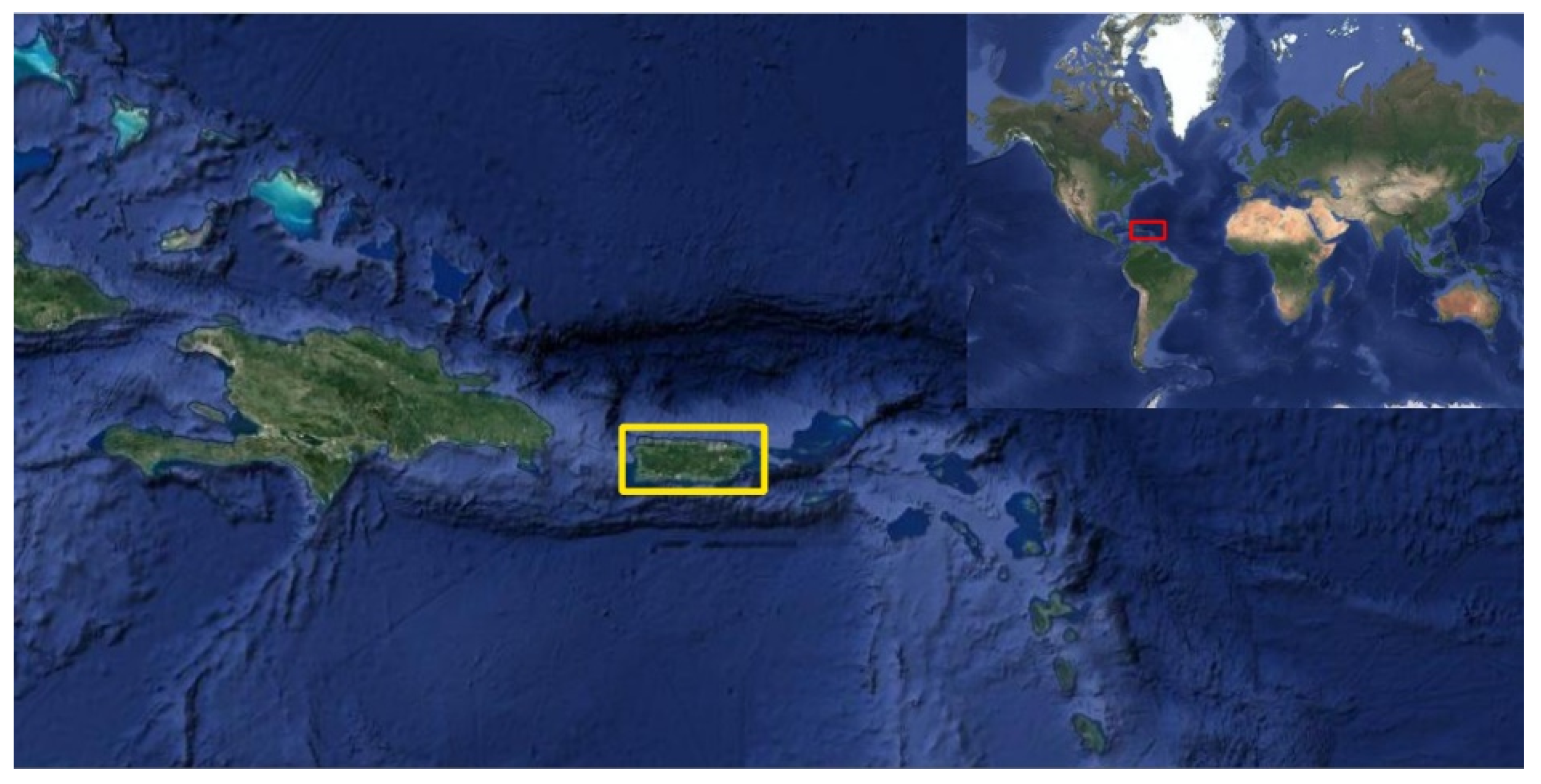
Figure 1. Location of PR. The red rectangle indicates the location of PR on the Earth, while the yellow rectangle shows the exact location of PR within the Caribbean Region.
Hydrology 08 00104 g001
Figure 2. Añasco watershed located in PR. Sub-watershed 1 represents the watershed area below the USGS stream discharge gauge, and Sub-watershed 2 represents the watershed area above the USGS stream discharge gauge.
Hydrology 08 00104 g002
Figure 3. Variation of the elevations within the study area.
Hydrology 08 00104 g003
Figure 4. (a) Land use land cover of the area of interest; (b) Soil Survey Geographic Dataset (SSURGO) for the Añasco watershed.
Hydrology 08 00104 g004
Figure 5. Flow chart summarizing the main steps.
Hydrology 08 00104 g005
Figure 6. 48 h cumulative rainfall from (a) WRF-simulated rainfall; (b) NWS rain gauge stations.
Hydrology 08 00104 g006
Figure 7. (a) WRF cumulative precipitation rainfall in millimeters over PR, (b) NWS cumulative rainfall in millimeters over PR, and (c) error in percentages between the WRF and NWS cumulative rainfall over PR.
Hydrology 08 00104 g007
Figure 8. (a) Observed (red points) and assumed (blue line) Hurricane María hydrograph for the USGS stream gauge located at San Sabastian, PR. (b) 48 h of the assumed Hurricane María. (Dates are in AST).
Hydrology 08 00104 g008
Figure 9. The NOAA tide station (9759394) monitoring at Mayaguez from 19 September at 12 pm to 21 September at 11 am of 2017 (AST); (a) Observed (red line) and predicted (blue line) storm surge during Hurricane María event; (b) Assumed storm surge for Hurricane María.
Hydrology 08 00104 g009
Figure 10. Location and depth in meters of the Survey data points over the lower area of the Añasco watershed (Sub-watershed 1).
Hydrology 08 00104 g010
Figure 11. Comparison between the modeled and observed (red line) hydrograph during Hurricane Irma using: (a) the calibrated parameters from the SLM calibration method (blue line); (b) the calibrated parameters from the MLSL calibration method (blue line).
Hydrology 08 00104 g011
Figure 12. Comparison between observed discharge (red line) and the modeled discharge using a time step of 2 (blue line) and 10 (green line) seconds for the rainfall event during 11–13 December 2007 (AST).
Hydrology 08 00104 g012
Figure 13. Hydrograph 1 is the output hydrograph at USGS stream discharge location using the WRF rainfall without any correction (blue line); Hydrograph 2 is the output hydrograph at USGS stream discharge location using the WRF corrected rainfall (red line).
Hydrology 08 00104 g013
Figure 14. Maximum flooding depth in Sub-watershed 1 using the observed USGS stream discharge data for Hurricane María as an inflow boundary condition and WRF rainfall. (a) Without incorporating storm surge; (b) including the storm surge.
Hydrology 08 00104 g014
Figure 15. Maximum flooding depth in Sub-watershed 1 using WRF rainfall for Hurricane María. Inflow hydrograph for Sub-watershed 1 was obtained by simulating runoff using WRF rainfall in Sub-watershed 2. (a) Without incorporating storm surge; (b) incorporating the storm surge.
Hydrology 08 00104 g015
Figure 16. Maximum flooding depth in Sub-watershed 1 using bias-corrected WRF rainfall for Hurricane María. Inflow hydrograph for Sub-watershed 1 was obtained by simulating runoff using bias-corrected WRF rainfall in Sub-watershed 2. (a) Without incorporating storm surge; (b) incorporating the storm surge.
Hydrology 08 00104 g016
Figure 17. Observed versus simulated flood depths using the USGS stream discharge data for Hurricane María as an inflow boundary condition and the WRF rainfall. (a) Without incorporating storm surge; (b) including the storm surge.
Hydrology 08 00104 g017
Figure 18. Observed versus simulated flood depths using WRF rainfall for Hurricane María. Inflow hydrograph for Sub-watershed 1 was obtained by simulating runoff using WRF rainfall in Sub-watershed 2. (a) Without incorporating storm surge; (b) incorporating the storm surge.
Hydrology 08 00104 g018
Figure 19. Observed versus simulated flood depths using WRF bias-corrected rainfall for Hurricane María. Inflow hydrograph for Sub-watershed 1 was obtained by simulating runoff using WRF bias-corrected rainfall in Sub-watershed 2. (a) Without incorporating storm surge; (b) incorporating the storm surge.
Hydrology 08 00104 g019
Figure 20. Maximum flood depth predicted using linear regression equation from Figure 17b and the maximum flood depth obtained from the observed USGS stream discharge data for Hurricane María as an inflow boundary condition, WRF rainfall and the storm surge; in addition, the storm surge was incorporated (HMA 2).
Hydrology 08 00104 g020
Figure 21. Maximum flood depth predicted using linear regression equation from Figure 18b and the maximum flooding depth in Sub-watershed 1 using WRF rainfall for Hurricane María; the inflow hydrograph for Sub-watershed 1 was obtained by simulating runoff using WRF rainfall in Sub-watershed 2. Additionally, the storm surge was incorporated (HMA 4).
Hydrology 08 00104 g021
Figure 22. Maximum flood depth predicted using linear regression equation (from Figure 19b) and the maximum flooding depth in Sub-watershed 1 using bias-corrected WRF rainfall for Hurricane María; the inflow hydrograph for Sub-watershed 1 was obtained by simulating runoff using bias-corrected WRF rainfall in Sub-watershed 2. Additionally, the storm surge was incorporated (HMA 6).
Hydrology 08 00104 g022
Figure 23. The red polygon represents the 500-year annual chance of flood hazard map taken from FEMA [81].
Hydrology 08 00104 g023
Table 1. Parameters selected during the calibration process and initial, minimum, and maximum values.
Parameters SelectedInitial ValueIntervals
MinimumMaximum
Channel Roughness 10.030.020.05
Channel Roughness 20.60.0510.075
Mixed Forest Roughness0.120.10.16
Hydraulic Conductivity for Clay0.030.020.06
Table 2. Comparison between the Hurricane Irma used in the calibration process and the Extreme Rainfall Event used in the validation process.
EventsDatesSpatial Resolution (m)Temporal Resolution (hr)Maximum Discharge Recorded in the Station (cms)Volume Hydrograph (USGS Station) (m3)Volume of Rainfall from NEXRAD (m3)
Sub-Watershed 2Sub-Watershed 1Sub-Watershed 2
Hurricane Irma9/6/2017 12:00–9/8/2017 11:00769159426,727,374.0013,337,01035,293,9530
Extreme Rainfall Event12/11/2007 00:00–12/13/2007 00:00632146822,888,190.00 9752,11329,394,120
Table 3. Volume comparison of the WRF and NWS interpolated rainfall.
Volume from Cumulative Rainfall (m3)Error (%)
WRF Cumulative RainfallNWS Interpolated RainfallAbsolute Difference (m3)
120,972,091185,939,47364,967,38234.94
Table 4. List of hydrologic modeling approaches (HMAs) used to simulate the flooding of Sub-watershed 1.
NumberHMAs
1USGS Hydrograph + WRF Rainfall + No Storm Surge
2USGS Hydrograph + WRF Rainfall + Storm Surge
3Inflow Hydrograph from Sub-watershed 2 using WRF Rainfall + WRF Rainfall + No Storm Surge
4Inflow Hydrograph from Sub-watershed 2 using WRF Rainfall + WRF Rainfall + Storm Surge
5Inflow Hydrograph from Sub-watershed 2 using bias-corrected WRF Rainfall + bias-corrected WRF Rainfall + No Storm Surge
6Inflow Hydrograph from Sub-watershed 2 using bias-corrected WRF Rainfall + bias-corrected WRF Rainfall + Storm Surge
Table 5. Type and total water, electrical, and public infrastructures.
InfrastructureTotal
Water infrastructureSewer pump stations33
Potable water pump stations40
Sewer plants1
Filtration Plants1
Wells12
Electric InfrastructureSubstations3
Transmission Center1
Public InfrastructurePublic Schools21
Table 6. Best parameters for each of the calibration methods.
ParametersSLMMLSL
Channel Roughness 10.020.02
Channel Roughness 20.0750.063
Mixed Forest Roughness0.10.1075
Hydraulic Conductivity for Clay0.020.02262
Table 7. Evaluation criteria results and comparison of the volume between the observed and modeled hydrograph for the SLM and MLSL method.
Evaluation MetricsVolume (m3)Evaluation Criteria
R2NSEPBIAS (%)ObservedModelledError (%)R2 > 0.6NSE > 0.5PBIAS < ±15%
SLM0.6130.5513.19726,727,37423,208,50613.2YesYesYes
MLSL0.5850.51915.6126,727,37422,563,22915.6NoYesNo
Table 8. Evaluation criteria results and comparison of the volume between the observed and modeled hydrograph using 2 s and 10 s time steps.
Evaluation MetricsVolume (m3)Evaluation Criteria
Time Step(s)R2NSEPBIAS (%)ObservedModelledError (%)R2 > 0.6NSE > 0.5PBIAS < ±15%
20.9460.903−1.8722,888,19023,328,9171.926YesYesYes
100.90.838−3.21122,888,19023,636,3193.269YesYesYes
Table 9. Comparison of the flood prone area from the 500-year annual chance of flood hazard map (FEMA) and the flooding maps of the different HMAs.
HMAFlooded Area (m2)Comparison with the FEMA Flood Extent Area
Absolute Difference (m2)Difference (%)
127,680,0007,109,370−20.44
227,920,0006,869,370−19.75
318,560,00016,229,370−46.65
418,740,00016,049,370−46.13
523,230,00011,559,370−33.23
623,370,00011,419,370−32.82
2 Corrected30,090,00046,99,370−13.51
4 Corrected23,810,00010,979,370−31.56
6 Corrected23,840,00010,949,370−31.47
Table 10. Water facilities that failed in each of the HMAs due to a flooding depth greater than 20 cm.
Water InfrastructureHMATotal Facilities
123456
Number of Facilities that Failed
Sewer pump stations9124771033
Potable water pump stations44444440
Sewer plants0000001
Filtration Plants0000001
Wells00002212
Table 11. Public and electrical infrastructures that failed in each of the HMAs due to a flooding depth greater than 20 cm.
Public and Electrical InfrastructureHMATotal Facilities
123456
Number of Facilities that Failed
Public Schools11001121
Substations0000003
Transmission Center0000001
Table 12. Water facilities that failed in HMAs 2, 4, and 6 using the linear regression approximation due to a flooding depth greater than 20 cm.
Water InfrastructureHMATotal Facilities
246
Number of Facilities that Failed
Sewer pump stations18131133
Potable water pump stations66640
Sewer plants0001
Filtration Plants0001
Wells33412
Table 13. Public and electrical infrastructures that failed in HMAs 2, 4, and 6 using the linear regression approximation due to a flooding depth greater than 20 cm.
Public and Electrical InfrastructureHMATotal Facilities
246
Number of Facilities that Failed
Public Schools43321
Substations0003
Transmission Center0001
Publisher’s Note: MDPI stays neutral with regard to jurisdictional claims in published maps and institutional affiliations.