A Model-Based Tool for Assessing the Impact of Land Use Change Scenarios on Flood Risk in Small-Scale River Systems—Part 2: Scenario-Based Flood Characteristics for the Planned State of Land Use

Abstract

Land use changes can significantly influence the water balance, and thus especially the development of flood-triggering runoff peaks. Hence, it is advisable to assess possible changes already at the level of municipal planning. Since many different actors are usually involved in spatial planning, it is useful to provide a shared platform where stakeholders can access the same information to analyze and evaluate flood hazards. Therefore, a GIS routine for the prediction of soil sealing induced runoff peaks and resulting potential flooding in the watercourse was developed, which is embedded in a GIS based decision support system (GIS-DSS). The so-called storm water routine (SWR) is founded on preprocessed flood characteristics, calculated by means of hydrological/hydraulic models (described in part 1). The potential impact of land use change is assessed purely in GIS as flow difference which is routed through the river system. To validate this simplified method, a process model was set up with an exemplary land use change and its results were compared with the GIS-based results. For 16 of the 18 rainfall scenarios tested, the SWR provided very good to good agreement with the detailed model. For short and highly dynamic rain events the SWR approach is less reliable. Several supplements like the integration of LID are conceivable.

1. Introduction

Since the beginning of human settlement history, humans have preferred to settle near rivers and streams. Small settlements became large settlements and these became today’s cities. As settlements progress, areas formerly close to nature are rezoned as building land and cities are redensified. This inevitably leads to increased soil sealing. Soil sealing strongly modifies the water cycle by reducing infiltration, evapotranspiration, and groundwater recharge, thus intensifying (rapid) surface runoff. As a result, the risk of flooding is increased [1,2] especially where no retention areas exist. For a region in China it has been shown that over the last 20 years urbanisation has led to an increase in the runoff coefficient of 13.4%, resulting in an increase in the maximum flood discharge of 12.9% on average [3]. In [4], a methodology is described which relates urban growth studies based on the analyzation of satellite data to distributed hydrological runoff modeling using the soil conservation service (SCS) method. The results of the corresponding case study indicate that annual runoff depth had increased by 8.10 mm between 1989 and 1997 due to urban sprawl.

The social and economic ‘costs’ of flooding are expected to rise in the future, not only due to land use changes, but also due to climate change [5,6,7]. In order to minimize flood risk by a proper communal planning, the impact of land use changes on runoff and river surcharge must be considered at an early stage. In this context, the cooperation and exchange of information between all relevant authorities, organisations, associations, and companies is of particular importance [8]. Typically, process models are applied for those questions. However, their application requires expert knowledge and detailed data, which are not available in this phase of planning.

The aim was therefore to develop a tool that enables a rapid, but still reliable assessment of flood risk due to land use change, which is applicable by regional planners or authorities without specific knowledge in hydrologic/hydraulic process modeling. The results shall be made available in a coherent way to all relevant actors across administrative boundaries. Due to the spatial nature of this issue, the use of a geo-information system (GIS) is appropriate. For a wide applicability, the tool shall be based on freely accessible software. Meanwhile, open source free software (namely QGIS) has achieved a technically mature level, “giving the researcher the ability to create their own tools, according to their needs” [9]. To provide an ideal solution for sharing basic data and calculation results, the tool shall be embedded in a GIS-based decision support system (GIS-DSS), accessible via a conventional web browser. Decision support systems have been developed since the 1970s [10] but the progressing digitalization and especially the free availability of geodata facilitates and improves the development enormously. In addition, powerful computers ensure faster real-time processing of geodata, which minimizes computing times. Many GIS-DSS were specifically designed for flood risk analysis and assessment [11,12,13,14]. However, to ensure that the DSS will be used by stakeholders once it has been developed, the following three key challenges must be met according to [15]:

• The DSS has to address the actual goals of the decision-makers and stakeholder wishes
• The DSS should provide a user-friendly interface and good visualization capabilities for a real participatory use by the stakeholders and decision-makers
• The stakeholder and decision-makers should have a clear understanding of the model concept and should ideally be able to edit it by themselves e.g., for scenario analysis purposes

There is a wide variety of approaches to address these, depending on the regarded topics, end-users and scientific background of the model developers. They reach from statistical and/or conceptual models processing meta information [16] to high resolute and well-considered 2D/3D flood risk mapping [17,18,19]. Partly, they are collaboratively developed with the end-users [20] or even use virtual reality environment to increase information depth and awareness. In tendency, the participatory character of the model decreases with increasing model accuracy. The concept of [16] is highly participative but does not provide physically exact information. Particularly, 3D maps are mainly prepared for citizens.

Our concept is ranging between these two edges: it is highly cooperative and based on deterministic physical modeling. More precisely, a tool was developed that allows an interactive calculation of the runoff from a particular planned land use and the subsequent propagation of the flow in the river system. The so called ‘storm water routine’ (SWR) was developed, as part of a larger GIS-DSS for regional and municipal planning activities [21]. The development is primarily based on open-source tools to enable barrier-free use by relevant stakeholders. It combines:

• a physical process model of the catchment hydrology and river hydraulics, set up for the current state of land use [22] and
• a GIS-routine calculating the additional runoff for land use change scenarios and its routing through the stream system.

The objectives of this tool have been defined in a participatory process with regional water authorities, water associations, and wastewater operators. They identified the lack of information on land use change induced changed runoff and missing information on specific hydraulic capacity at the point of discharge as major deficiencies in the approval of new storm water discharge permits. In distinct cases with expected larger impacts, individual studies are commissioned to consultancies, but a consistent and continuous assessment for a total river basin is missing. While most of the partners do not have their own modeling expertise, the application of GIS is meanwhile daily practice. GIS also provides the required visualization capabilities and interface for editing scenarios in the area of interest. Accordingly, it was agreed to develop a tool to holistically assess the hydrologic and hydraulic impacts of land use changes for the total river system. In contrast to commissioned studies, the tool should be operable and editable by the decision-makers and stakeholders themselves by using the well-known GIS environment. Since the tool is based on the pre-processed results of hydrologic/hydraulic models, but is not directly linked to the models, the end user does not necessarily need to have modeling experience.

While part 1 of this paper has described the set-up and parametrization of the process model and the definition of rainfall scenarios, this article focuses on the GIS-based calculation of additional runoff and the routing. The reliability of the approach has been reviewed by a comparative calculation of river flow with the detailed process model and the simplified GIS-based approach, revealing its strengths and weaknesses.

2. Materials and Methods

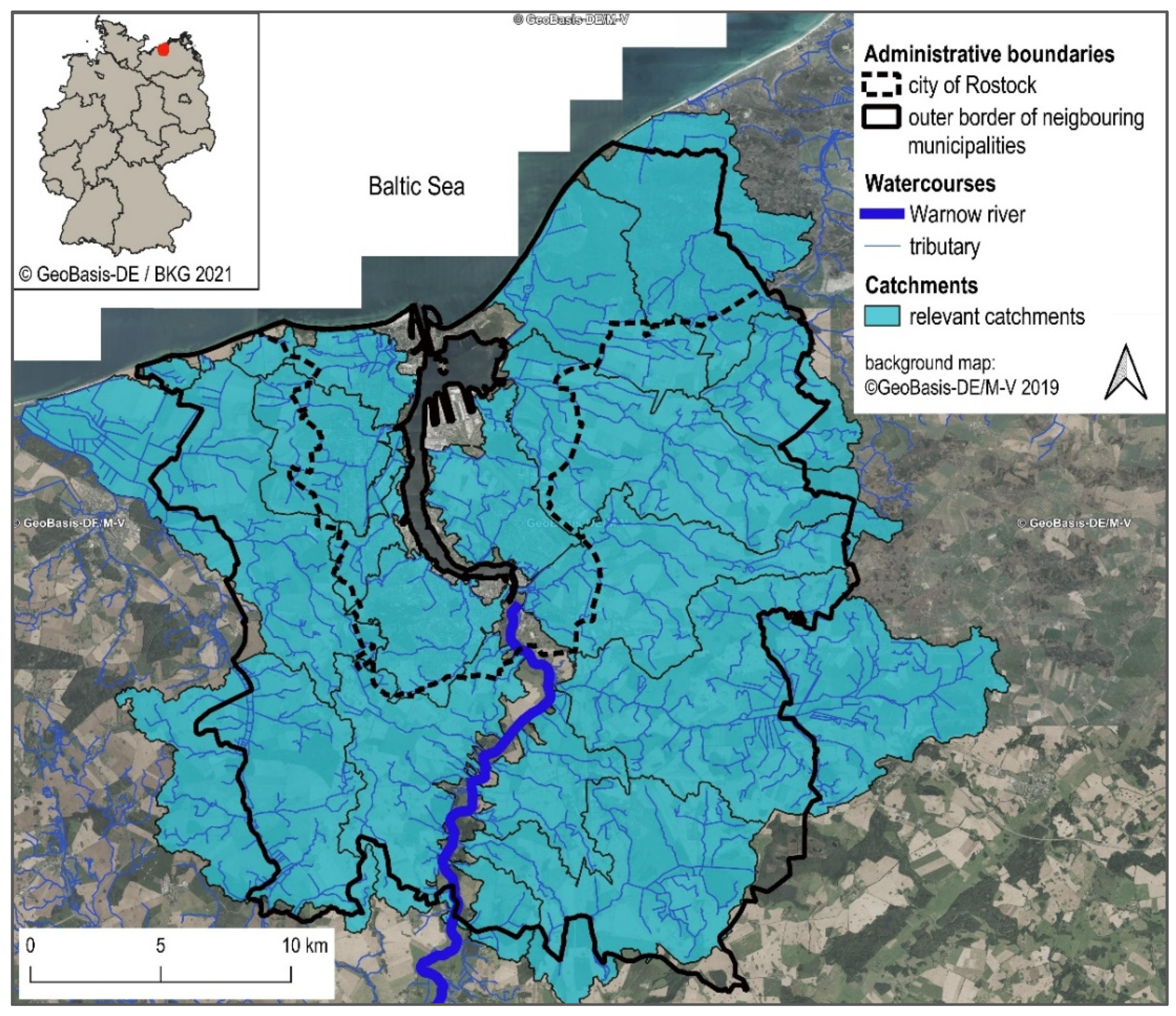
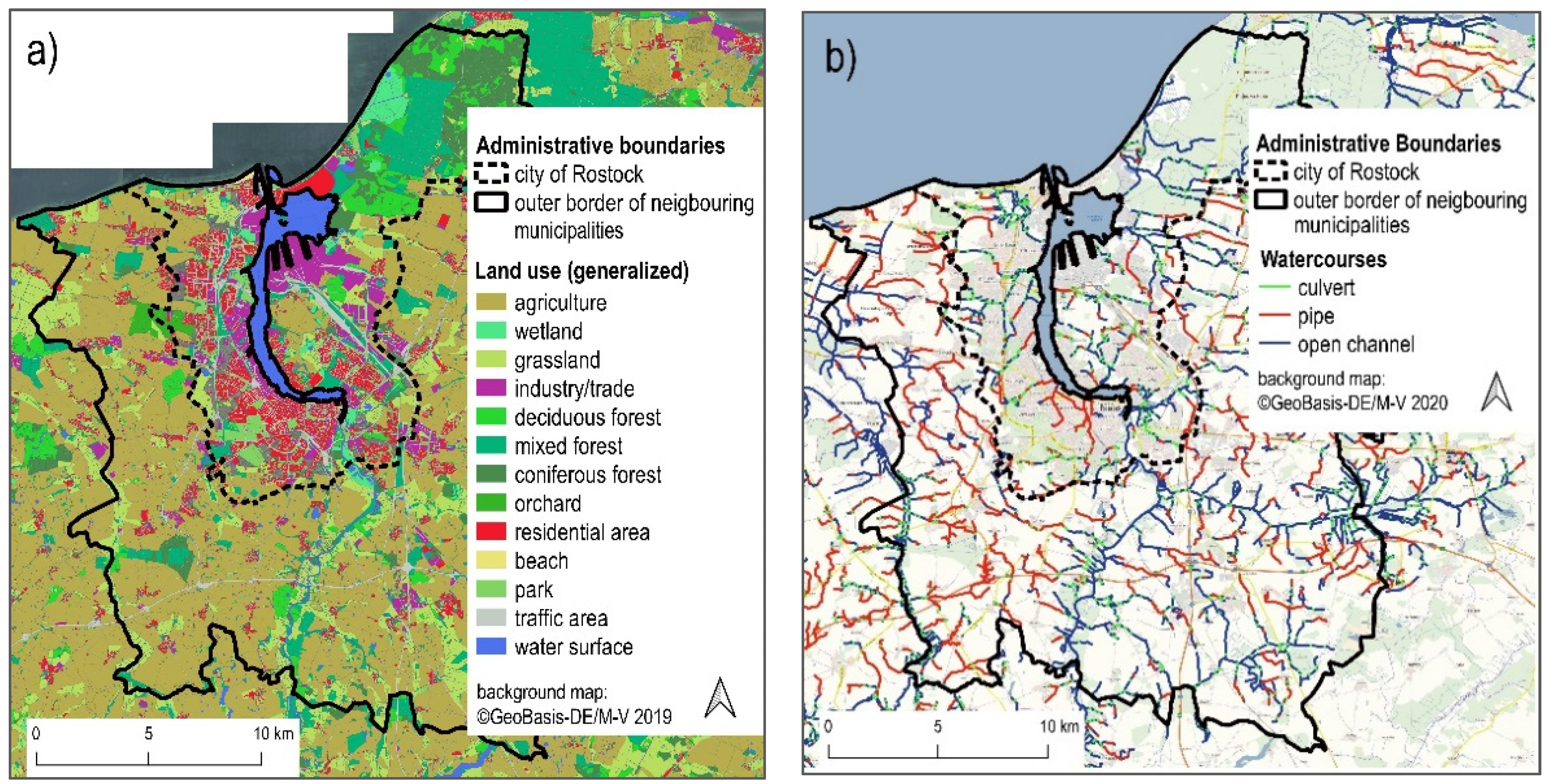
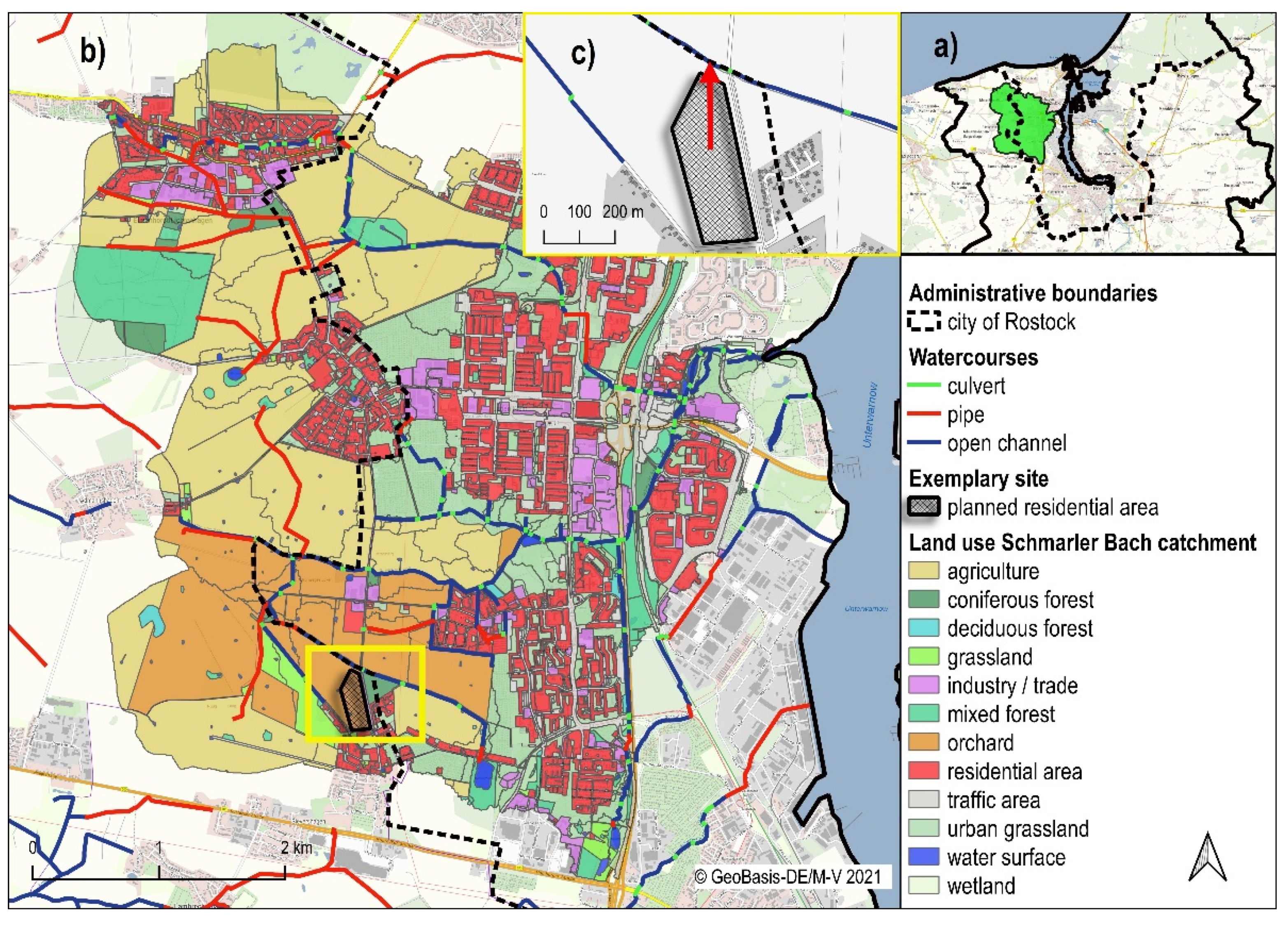
2.1. Study Area

The study area, approximately 530 km² in size, is located in the northeastern German lowlands and includes the Hanseatic City of Rostock and its 18 surrounding municipalities (Figure 1). The latter are part of the Rostock rural district. While the core of the city is dominated by uses such as housing, industry, and commerce as well as transport areas, the surrounding rural district is mainly characterised by arable land and grassland. The study area overlaps 19 largely independent surface catchments, with the headwaters of the streams mostly in the rural district and the mouths in the urban area of Rostock or the Baltic Sea.

The history of the city of Rostock goes back to the 13th century. Since then, the city has grown not only in its territorial area but also in its population, reaching nearly 210.000 inhabitants today [23]. For Rostock, an increase of nearly 15.000 inhabitants is expected by 2035 [24]. In contrast, projections indicate that the rural district will experience a population decline of 1.8% by 2030 [25]. However, as in many developed countries, population and sealing do not develop in parallel, but the demand for building ground is increasing, even in areas with shrinking population. Main drivers are the demand for residential units, the development of logistic centers and industrial parks.

2.2. Basic Data

In the course of the study, spatial data from different sources were used and integrated into a homogeneous and consistent data set. The data relevant for the application of the storm water routine are presented in the following.

2.2.1. Land Use Map

The Hanseatic City of Rostock provides a spatially high-resolution geodata set that was created on the basis of aerial photographs and supplemented by existing geodata. Since such a dataset did not exist for the rural district, it was generated from the data of the Official Real Estate Cadastre Information System (German abbreviation: ALKIS) in combination with satellite data. The result is a polygon shape file that depicts the land use in its actual state on the basis of 48 classes. In the GIS-DSS, this land use map represents the reference state for all future changes of land use. In addition, different levels of protection (risk classes) were defined for each land use class according to their vulnerability (see [22]). The level of protection is expressed by the return period which describes the probability of recurrence of a natural event, in this case a statistical model rainfall of a certain duration. For hydrologic/hydraulic modeling [22], the 48 classes were generalized to 13 land use classes (Figure 2a).

2.2.2. Watercourse Cadastre

The watercourse cadastre contains stream networks (Figure 2b) and their catchments (Figure 2c). The watercourse lines were brought together from several different sources and corrected in order to create a tree structure. Thus, each tributary flows to a receiving stream and is connected to it at a certain point. These hierarchical routes were divided into 50 m sections and equipped with an individual and hierarchical identification number (12-digit watercourse identification number: WIN) and chainage.

Each watercourse was assigned a surface catchment. These were calculated on the basis of a digital elevation model (DEM) with a cell size of 5 m. The stream catchments were also further subdivided so that each 50 m section is assigned its own subcatchment. Due to the strict hierarchy of both watercourses and catchments, which is maintained by means of the WIN, sections or subcatchments located upstream or downstream can be quickly identified and aggregated if necessary [26].

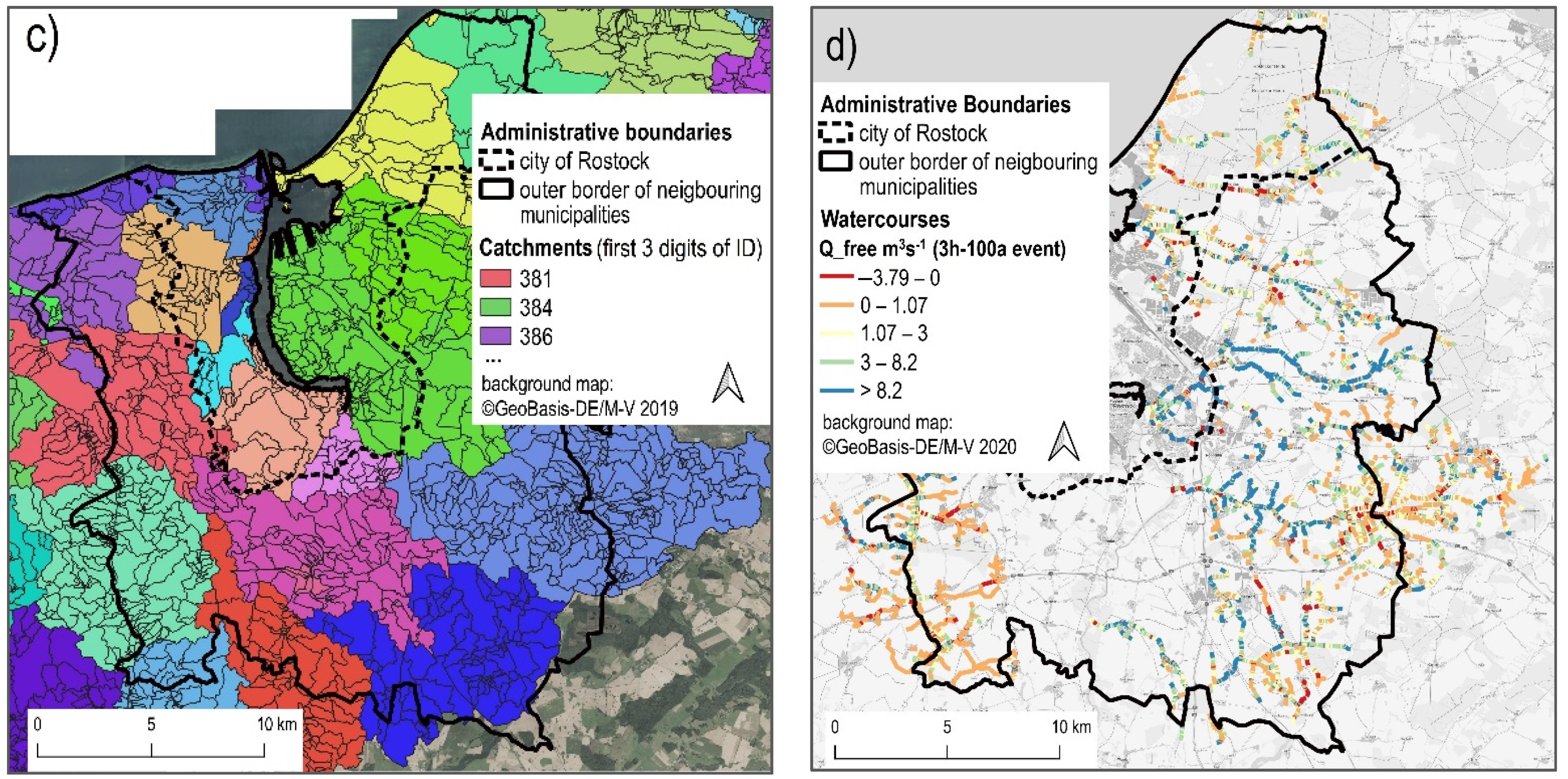
2.2.3. Flood Characteristics

For the watercourses and catchments of the study area, spatially high-resolution flood characteristics for the current state were preprocessed using combined rainfall-runoff and hydrodynamic stream models [22]. The flood characteristics are available for 18 precipitation events of different durations and return periods (see

Table 1. Selected statistical precipitation events according to protection level of land use classes ([22], modified).

Duration	Return Period
1 h	2 a, 100 a
3 h	10 a, 25 a, 50 a, 100 a
6 h	10 a, 25 a, 50 a, 100 a
9 h	10 a, 25 a, 50 a, 100 a
12 h	10 a, 25 a, 50 a, 100 a

).

The return period expresses the level of protection that has been defined for a particular land use class [27]. For example, if a return period of 100 a has been defined for a residential area, the area should not be flooded by a rainfall event that statistically occurs every 100 a. However, for reasons of economic efficiency, the area is allowed to be flooded by an even rarer and thus larger event. In order to detect the worst case, different durations were taken into account, as long rainfall durations are usually critical for large areas and shorter durations are relevant for smaller areas with shorter flow paths.

Table 2. Flood characteristics for the actual state applied in the SWR based on scenario simulations with defined rain events.

	Designation	Unit	Declaration
Watercourses	Qfull	m3 s−1	Maximum possible flow at normal flow (water level gradient = bottom gradient)
	Qmax,act	m3 s−1	Maximum flow
	Qfree,act	m3 s−1	Flow rate that would additionally fit into the cross profile at maximum flow rate; value calculated from model results (Figure 2d): Qfree,act = Qfull − Qmax,act
Subcatchments	Rmax,act	m3 s−1	Maximum direct runoff (surface runoff)

shows the preprocessed flood characteristics used in the storm water routine of the DSS.

2.2.4. Maximum Rainfall Intensities

Within the framework of the heavy rainfall regionalisation, the KOSTRA Atlas of the German Weather Service provides precipitation amounts as a function of duration D and annuality T (return period) [28]. While a block rain was assumed for the duration stages greater than or equal to 3 h, the intensity course for the duration stage 1 h was determined statistically based on DWA-A 118 [29] and includes a clear rain peak after about half of the time. The resulting maximum rainfall intensities ($r{i}_{max}$) were listed in tabular form and linked to the geodata of the hydrologic catchments.

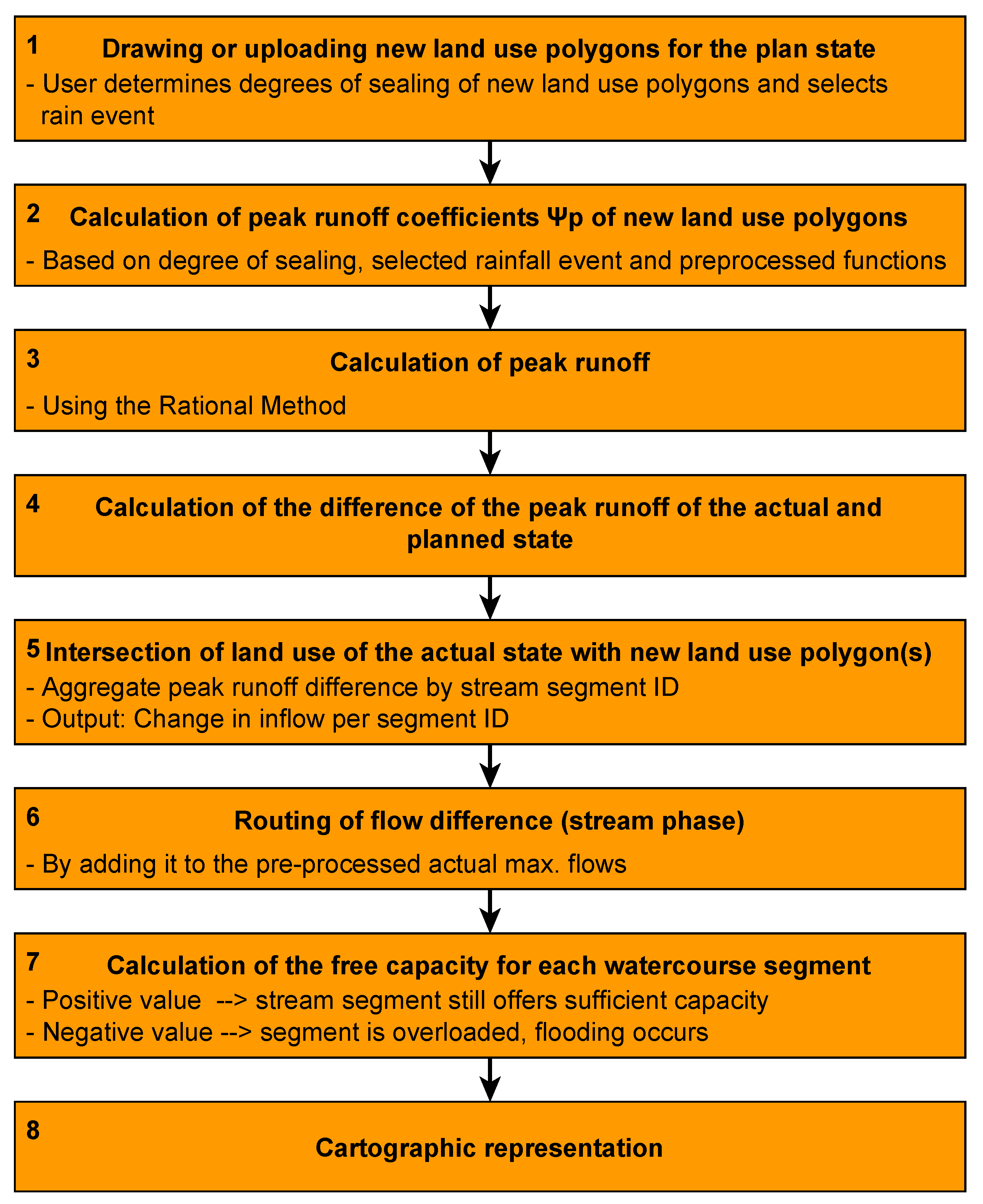
2.3. Detection of Flood Characteristics for Planned Land Use Changes

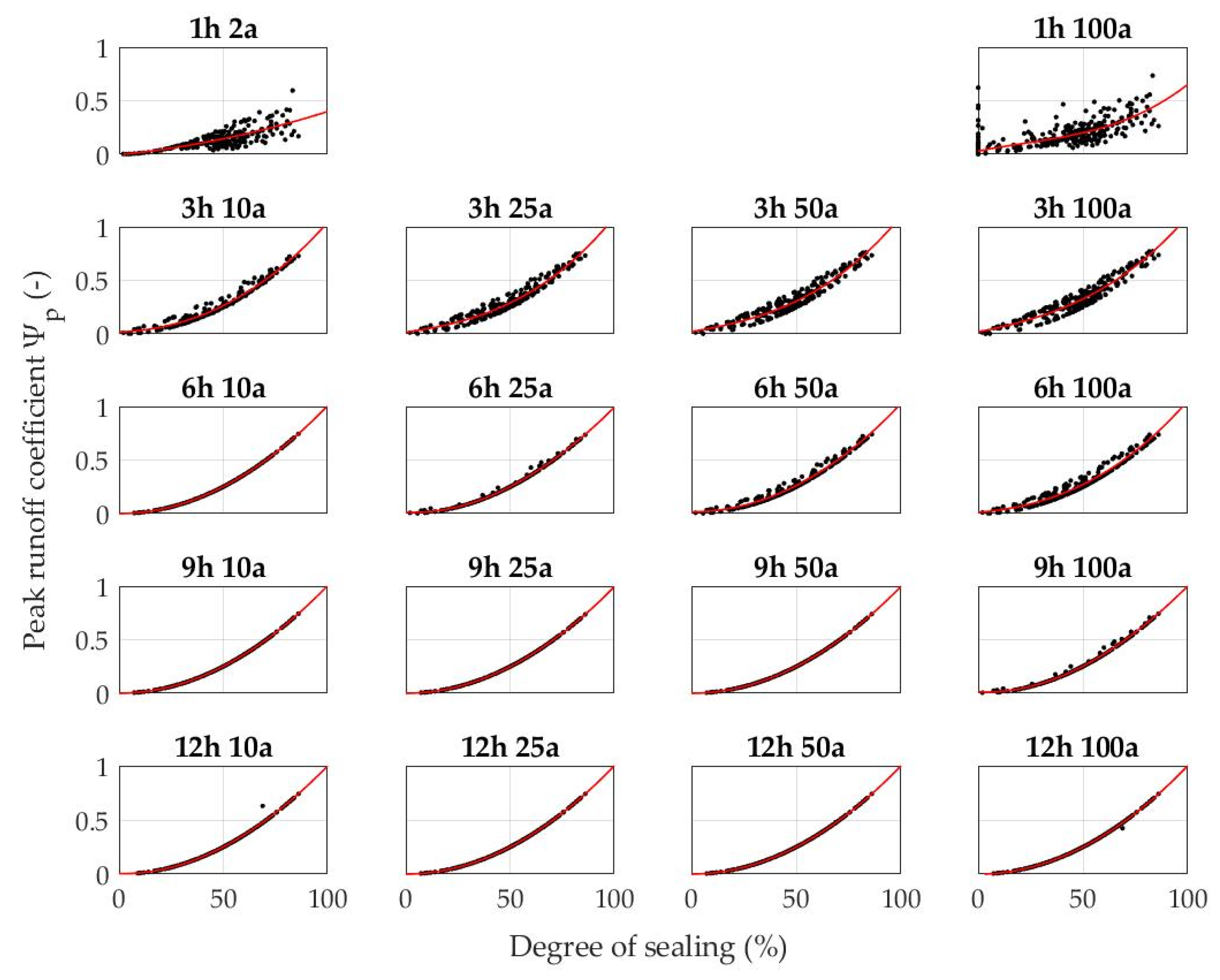
2.3.1. Pre-Processing of Functions to Calculate Peak Runoff Coefficients

For the development of the storm water routine, functions were derived beforehand on the basis of the existing model results (see Table 2), which enable the calculation of the peak runoff coefficient for new land use polygons on the basis of a specified degree of sealing. In the first step, the peak runoff coefficients are determined for each subcatchment of a reference model site (Schmarler Bach site, see [22]) for the 18 simulated model rainfall events. The coefficient describes the ratio of the maximum runoff rate per area to the corresponding maximum rainfall rate per area (Equation (1)) and depends primarily on the proportion of paved areas (degree of sealing), the slope of the terrain and the rainfall intensity [29]. As the study area is located in the lowlands, the gradient plays a minor role here. This was supported by the model results, as the dependence of the coefficient on the gradient was tested and evaluated as not significant.

$${\mathsf{\Psi }}_p=\frac{r_{max}}{r{i}_{max}}$$

(1)

$${\mathsf{\Psi }}_p=peak runoff coefficient (-)$$

$$r_{max}=maximum runoff rate per area \left(\mathrm{l} {\mathrm{s}}^{-1} {\mathrm{m}}^{-2}\right)$$

$$r{i}_{max}=maximum rainfall intensity per area \left(\mathrm{l} {\mathrm{s}}^{-1} {\mathrm{m}}^{-2}\right)$$

Subsequently, a comparison of the peak runoff coefficients and the degrees of sealing was performed in a correlation diagram. Thereby polynomial functions were derived, which describe the correlation between the two parameters. The functions are used to calculate the peak runoff coefficient for a new land use polygon on the basis of the defined degree of sealing and the selected rainfall scenario.

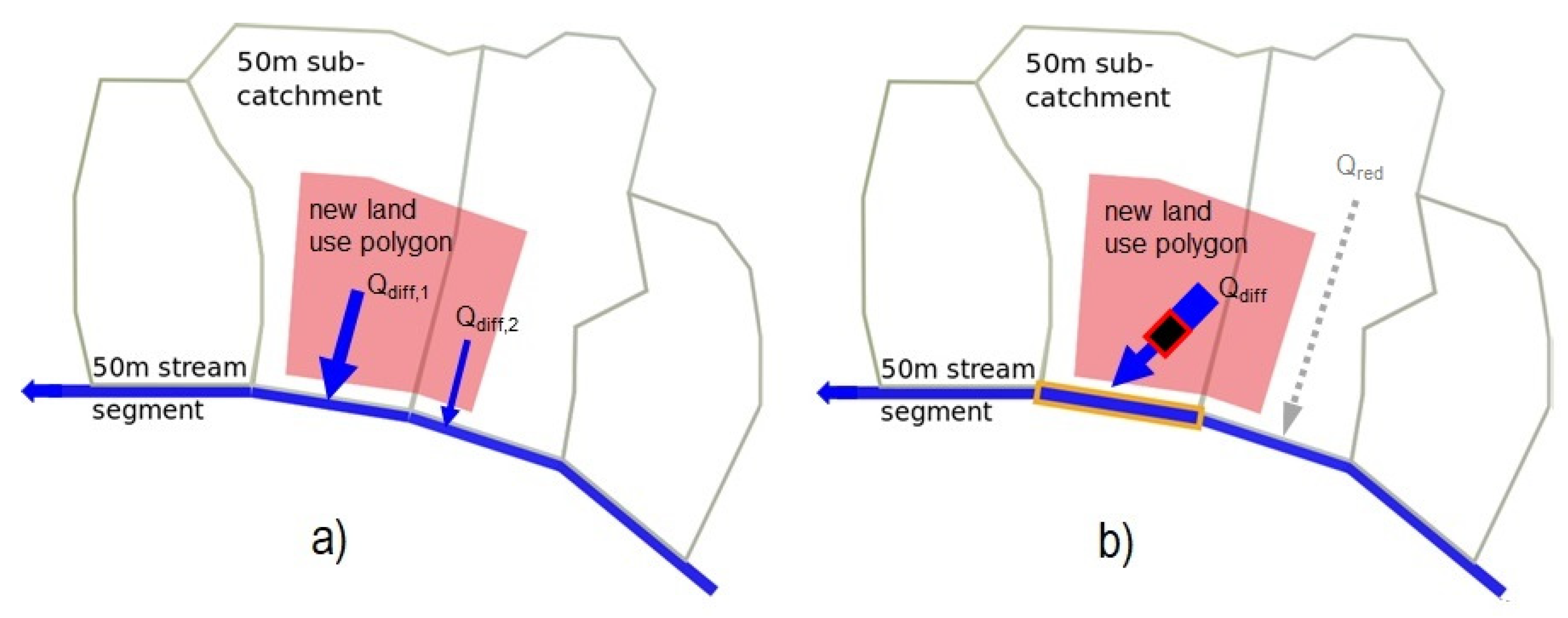
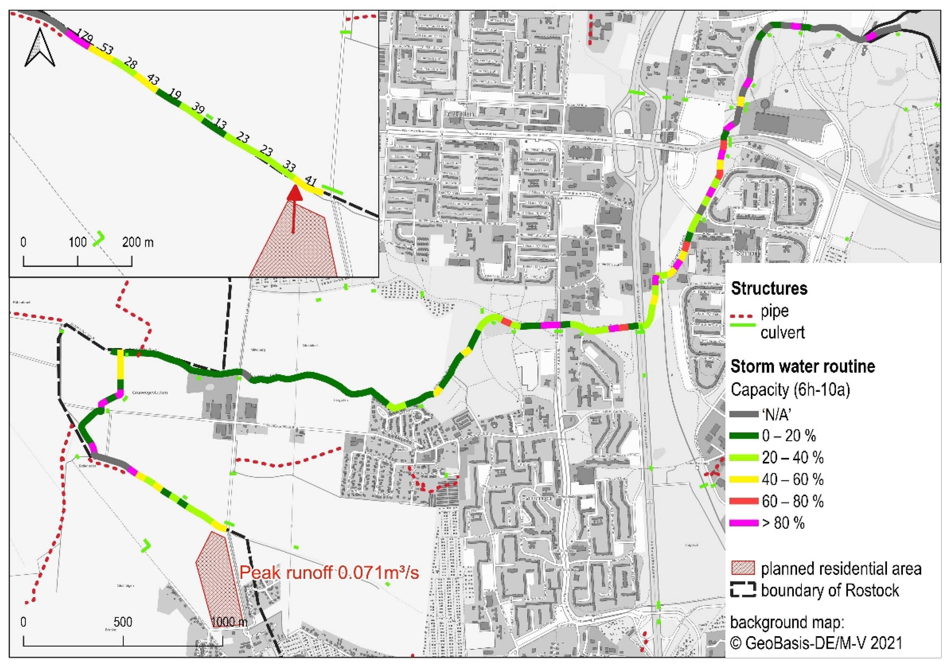
2.3.2. The Storm Water Routine

The storm water routine aims to provide potential future runoff and flood risk associated with planned land use changes. For this purpose, a method was developed that enables the calculation of the direct runoff and resulting potential flows for planned land uses on the basis of pre-processed flood characteristics. The procedure takes place in the Web GIS-DSS and is divided into eight basic steps (Figure 3). These were automated using Python programming language.

In the first step, a new land use polygon is either directly drawn into the map of the graphical user interface or uploaded as a shape file. In this process, the user specifies the planned degree of sealing and selects the precipitation scenario with the corresponding maximum rainfall intensity per area. For the determination of the peak runoff coefficient, preprocessed polynomial functions were used that allow a calculation based on the degree of sealing. The peak runoff $R_{max,plan}$ for the new land use polygon can thus be determined with the equation

$$R_{max,plan}={\mathsf{\Psi }}_p\times r{i}_{max}\times A_{new}$$

(2)

$$R_{max,plan}=maximum runoff rate in plan state\left(\mathrm{l} {\mathrm{s}}^{-1}\right)$$

$$A_{new}=area of new polygon \left({\mathrm{m}}^2\right)$$

The change in the peak runoff of the affected areas is computed by intersecting the maximum runoff of the actual land use (results from scenario simulations, see Table 2) with the maximum runoff of the new polygon both in raster format. For this purpose, the runoff rates are converted into runoff rates per raster cell (with a size of 100 m²).

$$r_{diff}=r_{max, plan}-r_{max, act}$$

(3)

$$r_{diff}=runoff rate difference per pixel \left(\mathrm{l} {\mathrm{s}}^{-1}100{\mathrm{m}}^{-2}\right)$$

in which:

$$r_{max,plan}=\frac{R_{max,plan}}{{\mathrm{A}}_{SC}}\times 100$$

(4)

$$r_{max,act}=\frac{R_{max,act}}{{\mathrm{A}}_{SC}}\times 100$$

(5)

$$r_{max,plan}=maximum runoff rate per pixel in plan state \left(\mathrm{l} {\mathrm{s}}^{-1}100{\mathrm{m}}^{-2}\right)$$

$$r_{max,act}=maximum runoff rate per pixel in actual state \left(\mathrm{l} {\mathrm{s}}^{-1}100{\mathrm{m}}^{-2}\right)$$

$${\mathrm{A}}_{SC}=area of corresponding subcatchment \left({\mathrm{m}}^2\right)$$

After intersecting the new polygon with the 50 m subcatchments, the change of peak runoff can finally be aggregated by segment ID and thus assigned to each receiving stream segment. There are two possibilities for the allocation of the runoff: (a) If no receiving segment is specified, the discharge is automatically distributed to the segments according to its area share in the subcatchment (Figure 4a,b) It is also possible to assign the discharge change to a defined segment and to throttle it via a maximum permissible discharge (Figure 4b). In the case of Figure 4b, the corresponding stream segment receives the peak runoff difference and the neighbouring upstream segment loses runoff compared to the actual state (Q_red) due to the reduced drained area.

The new inflow (Q_diff) is added to the maximum stream flow of the actual state (Q_max,act) and routed downstream according to the WIN

$$Q_{max,plan}=Q_{max,act}+Q_{diff}$$

(6)

$$Q_{max,plan}=maximum flow in plan state \left(\mathrm{l} {\mathrm{s}}^{-1}\right)$$

$$Q_{max,act}=maximum flow in actual state \left(\mathrm{l} {\mathrm{s}}^{-1}\right)$$

$$Q_{diff}=aggregated runoff difference \left(\mathrm{l} {\mathrm{s}}^{-1}\right)$$

From the full flow (Q_full, Table 2), which represents the maximum possible flow for a specific cross profile, and the new flow of the planned state (Q_max,plan), the flow that would still fit into the profile (Q_free,plan) is determined. If the value is positive, the profile still offers enough capacity for the additional flow. If it is negative, the segment is overloaded and flooding occurs.

$$Q_{free,plan}=Q_{full}-Q_{max,plan}$$

(7)

$$Q_{free,plan}=flow, that would still fit in profile in plan state \left(\mathrm{l} {\mathrm{s}}^{-1}\right)$$

$$Q_{max,act}=maximum flow in actual state \left(\mathrm{l} {\mathrm{s}}^{-1}\right)$$

Both the stream flows for the 50 m segments as well as the capacities of the planned state are mapped in the GIS-DSS. For the visualisation, the line width is adjusted according to the total flow. As well, six colour levels have been assigned for the capacity to indicate how much space the profile still offers or whether it is already overloaded.

2.4. Validation of the Storm Water Routine

The validation of the storm water routine was performed by comparing its results for an exemplary land use change with the corresponding results from the combined hydrological/hydraulic model in SWMM. SWMM was considered to be a suitable benchmark, as it takes water body shapes at individual points into account and is able to calculate precisely dynamics of the flow, including effects of throttling and retention [22].

The exemplary land use change is the conversion of almost 70.000 m² of an orchard into a virtually planned residential area (‘planned area’) with a degree of sealing of 70%. The site is located in the catchment of the Schmarler Bach in the north-west of the investigation area (Figure 5a). Within the catchment area, the site is located in the southern-central part, just beyond the city boundary in the administrative area of the rural district (Figure 5b).

The discharge point into the river is set to a user-defined stream segment (red arrow in Figure 5c) as described in Figure 4b. Hence, the new residential area will drain in northern direction towards the open ditch just below the culvert (Figure 5b,c). On the flow path towards the mouth into the Warnow River, numerous structures such as culverts and pipes act as throttling elements in particular at high flows.

For the validation, representative precipitation scenarios were tested (cf. Table 1). The comparison between SWR and hydrological/hydraulic model was conducted for peak runoff from the development site, peak flows in the affected river sections.

3. Results

3.1. Derived Functions for the Determination of Peak Runoff Coefficients

Using the simulation results for the maximum surface runoff and the maximum rainfall intensity, the peak runoff coefficients for the current state were calculated according to Equation (1). Figure 6 shows the correlation of the peak runoff coefficient and the degree of sealing. Functions for the determination of the peak runoff coefficients on the basis of the degree of sealing are displayed in

Table 3. Functions relevant for the study area for the determination of the peak runoff coefficient ${\mathsf{\Psi }}_p$ (y) on the basis of the degree of sealing (x).

		Return Period
		2a	10a	25a	50a	100a
Duration	1 h	y = 1E − 07 × 3 + 1E − 05x2 + 2.1E − 03x				y = 1E − 06x3 − 9E − 05x2 + 6.2E − 03x
	3 h		y = 4E − 07x3 + 4E − 05x2 + 2.1E − 03x	y = 7E − 07x3 + 6E − 07x2 +4E − 03x	y = 8E − 07x3 − 1E − 05x2 + 4.8E − 03x	y = 7E − 07x3 − 1E − 05x2 + 5.4E − 03x
	6 h		y = −2E − 10x3 + 1.0E − 04x2 + 5E − 08x	y = 3E − 08x3 + 1E − 04x2 + 2.0E − 04x	y = 2E − 07x3 + 7E − 05x2 + 1.2E − 03x	y = 4E − 07x3 + 4E − 05x2 + 2.4E − 03x
	9 h		y = 1E − 11x3 + 1.0E − 04x2 + 5E − 08x	y = 1E − 11x3 + 1E − 04x2 + 3E − 08x	y = 8E − 12x3 + 1E − 04x2 + 3E − 08x	y = 2E − 08x3 + 1E − 04x2 + 9E − 05x
	12 h		y = −2E − 08x3 + 1.0E − 04x2 − 1.0E − 04x	y = −5E − 12x3 + 1.0E − 04x2 − 3E − 08x	y = −7E − 10x3 + 1.0E − 04x2 − 3E − 06x	y = 7E − 09x3 + 1E − 04x2 + 3E − 05x

. These are used in the storm water routine to determine peak discharges for planned land use changes.

Basically, a clear polynomial dependence of the peak runoff coefficients on the degree of sealing is visible. This is also confirmed by the coefficients of determination in

Table 4. Corresponding coefficients of determination R2 (-) for the simulated rain events.

		Return Period
		2 a	10 a	25 a	50 a	100 a
Duration	1 h	0.601				0.658
	3 h		0.972	0.945	0.929	0.918
	6 h		1.000	0.997	0.982	0.960
	9 h		1.000	1.000	1.000	0.997
	12 h		0.996	1.000	1.000	1.000

. In the case of block rainfall (3 h to 12 h), the strength of the dependency increases with duration, as conditions become more and more static. Within a duration category, the dependency tends to decrease from small to large return periods (respectively small to large rain intensities). For the duration 1 h with a clear intensity gradient, the scatter of the peak runoff coefficients around the function curve is significantly greater than for the block rainfall, which suggests that other factors, such as the area size or the flow length or the soil conductivity, superimpose the influence of the degree of sealing. In the case of the most severe event (1 h–100 a), it is noticeable that even the unsealed areas react as if they were sealed, since the conductivity of the soil is increasingly exceeded.

3.2. Validation of the GIS-DSS Storm Water Routine

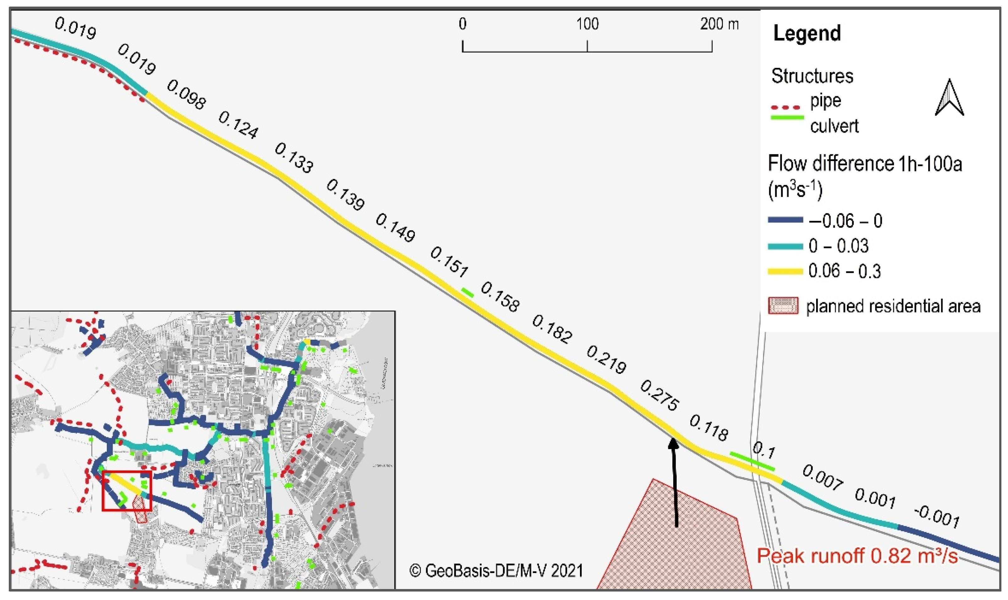
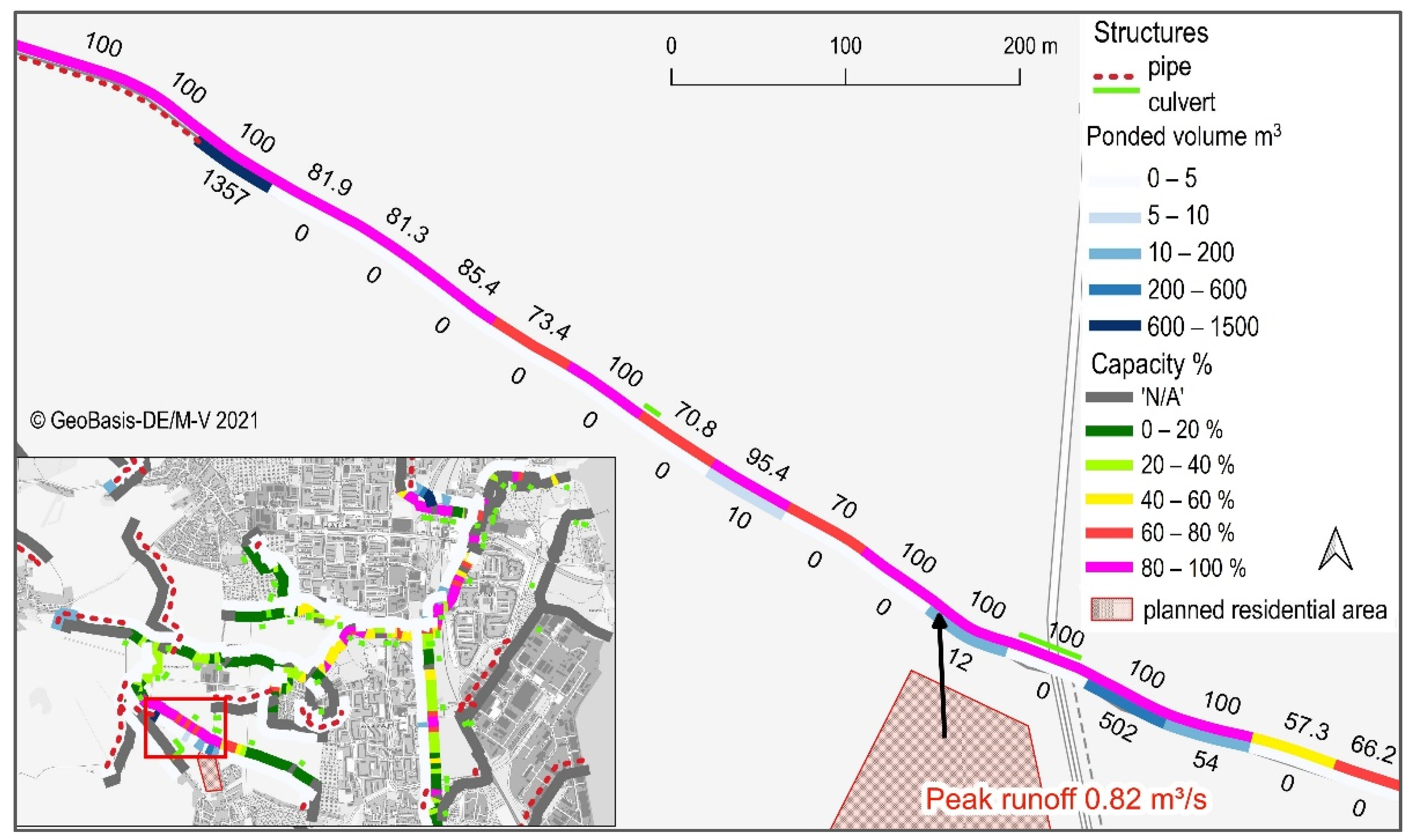
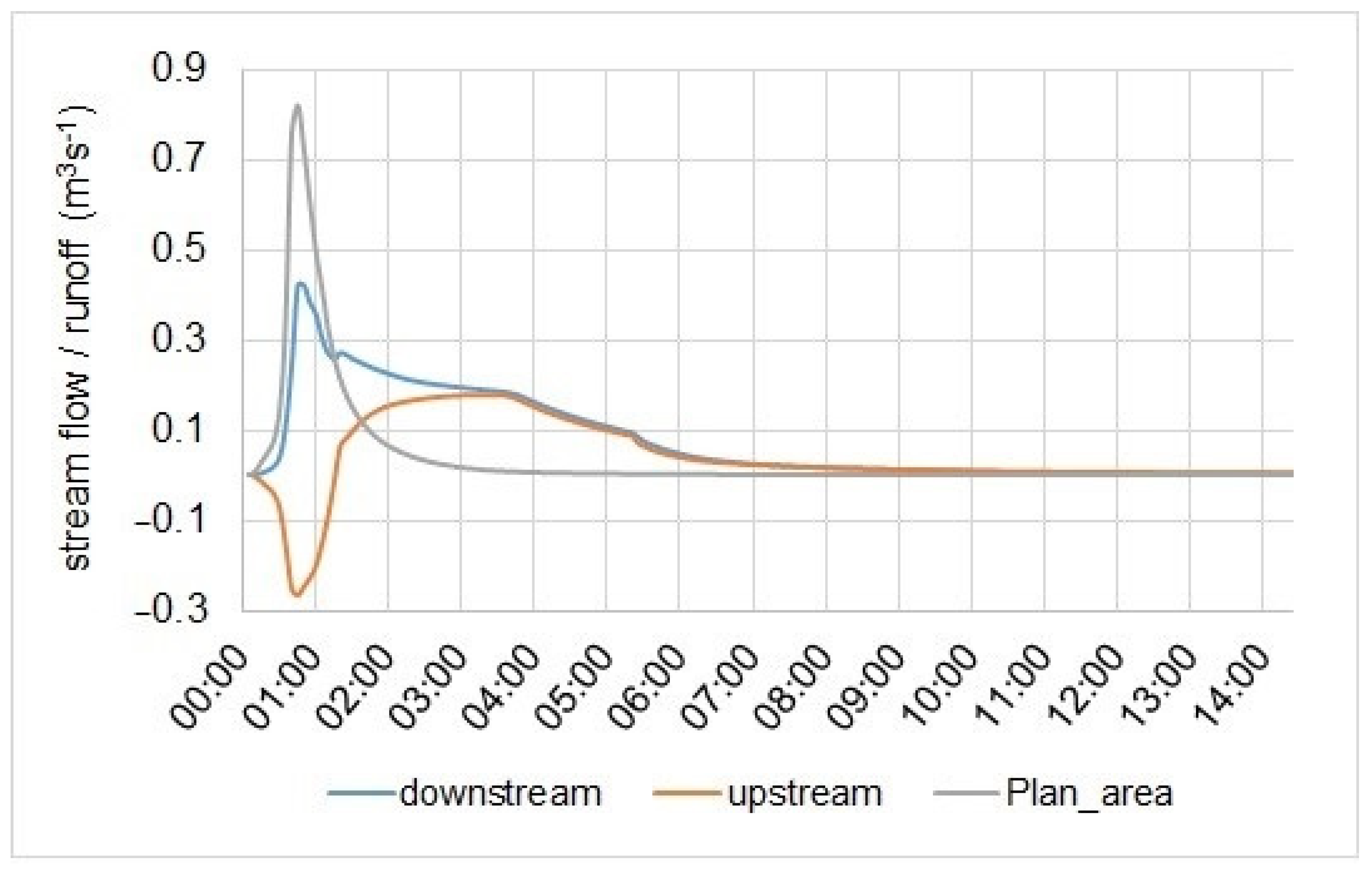
3.2.1. Comparison of Model Results for Actual and Plan State in SWMM

In order to better interpret and evaluate the results of the GIS-DSS storm water routine, this section first compares the model results for the current and the planned state. To start with a less extreme event, Figure 7 shows the difference in flows (Q_max,plan − Q_max,_act) in the planned and actual state for the rainfall event 6h-10a simulated with SWMM. The turquoise and yellow sections show on which stretches the discharge change has an effect.

As expected, the largest differences in stream flow occur immediately downstream of the discharge point and are of the same magnitude as the peak runoff from the planned area (Figure 8). At the same time, the new runoff also affects an approx. 130 m long stretch upstream of the discharge point but with a less prominent amplitude.

With downstream distance from the discharge point, the flow difference flattens from 0.071 m³s⁻¹ to 0.062 m³s⁻¹, which can be explained by the natural retention of an open channel. A pipeline section follows, which is about 95% full in the actual state, but already overloaded in the planned state. As a result, the flows are noticeably throttled here, which is why the additional discharge of the new residential area from this section onwards has relatively little effect.

A much more intense event is the 1h-100a rainfall (Figure 9 and Figure 10). Here, 0.82 m³s⁻¹ of runoff is generated on the new residential site. Since the profile downstream can only capture 0.42 m³s⁻¹, the conduits capacity limit is already reached. However, due to the rise in water level in the area of the discharge point and the resulting inversion of the upstream gradient, water flows in both directions: 0.42 m³s⁻¹ flows downstream and approx. 0.26 m³s⁻¹ flows upstream (Figure 11).

The remaining discharge (approximately 0.14 m³s⁻¹) is excess water and is temporarily stored in a conceptual reservoir above the banks. In SWMM, this is called the ponded volume. The speed with which the water flows out of the reservoir back into the cross-section depends on the size of the base area of the reservoir. If the surface area is small, the hydraulic pressure in the reservoir is relatively high and the water flows back again correspondingly quickly. This in return influences the shape and the maximum value of the stream flow. Since the study area is located in the lowlands, the footprint of the reservoir was chosen to be relatively large (distance to the next cross section below multiplied by 40 m). However, this conceptual approach has uncertainties from the moment flooding occurs.

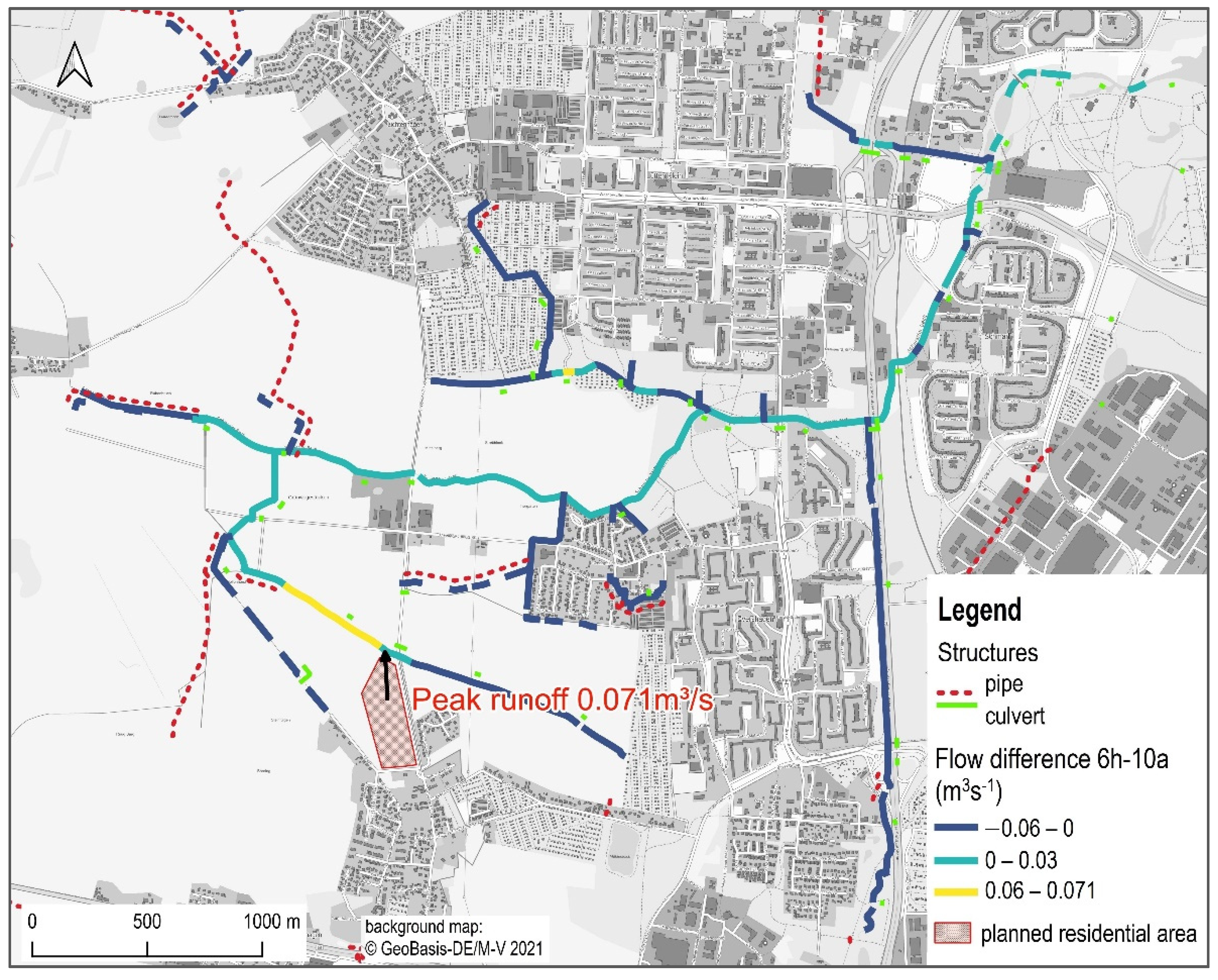
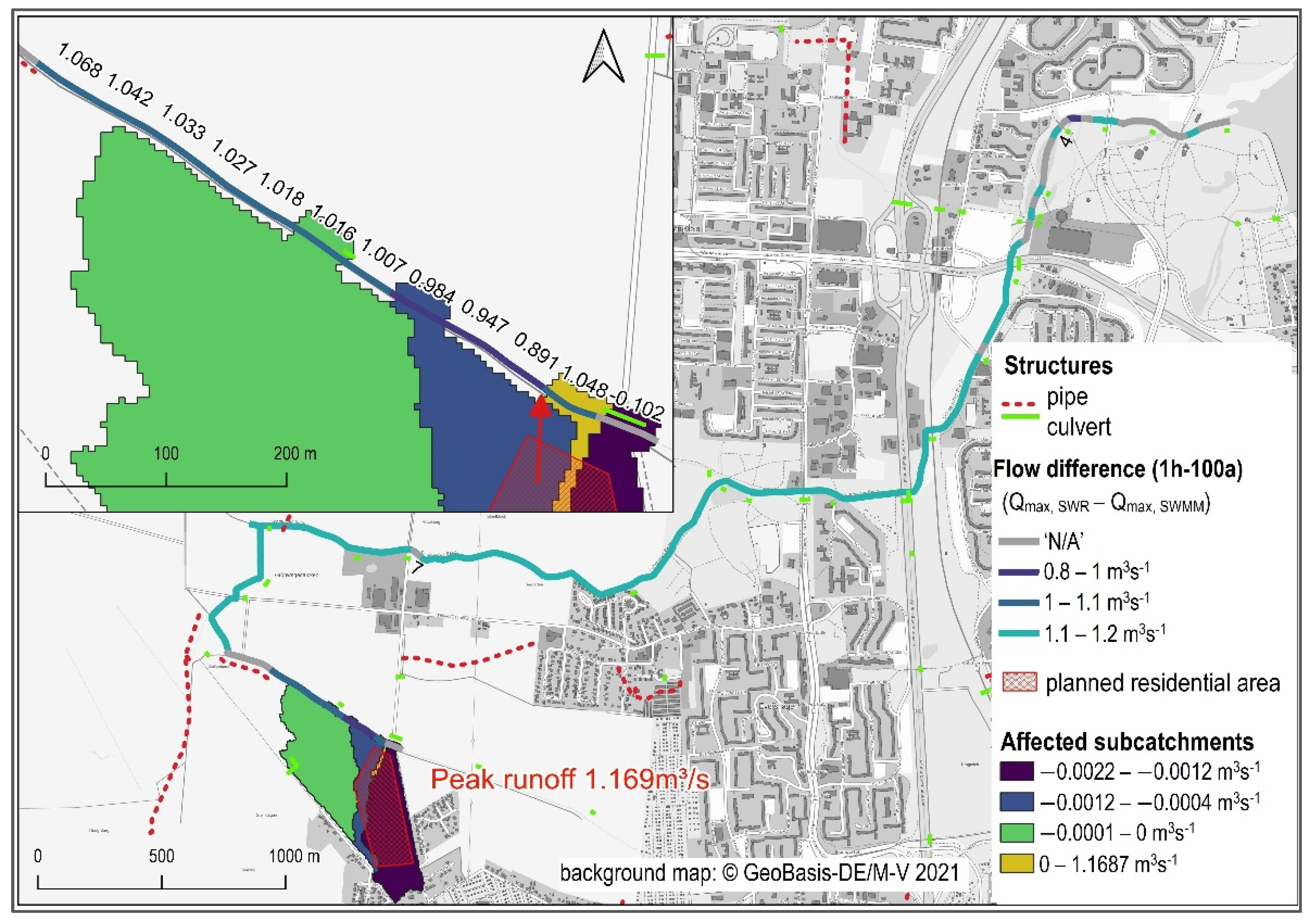
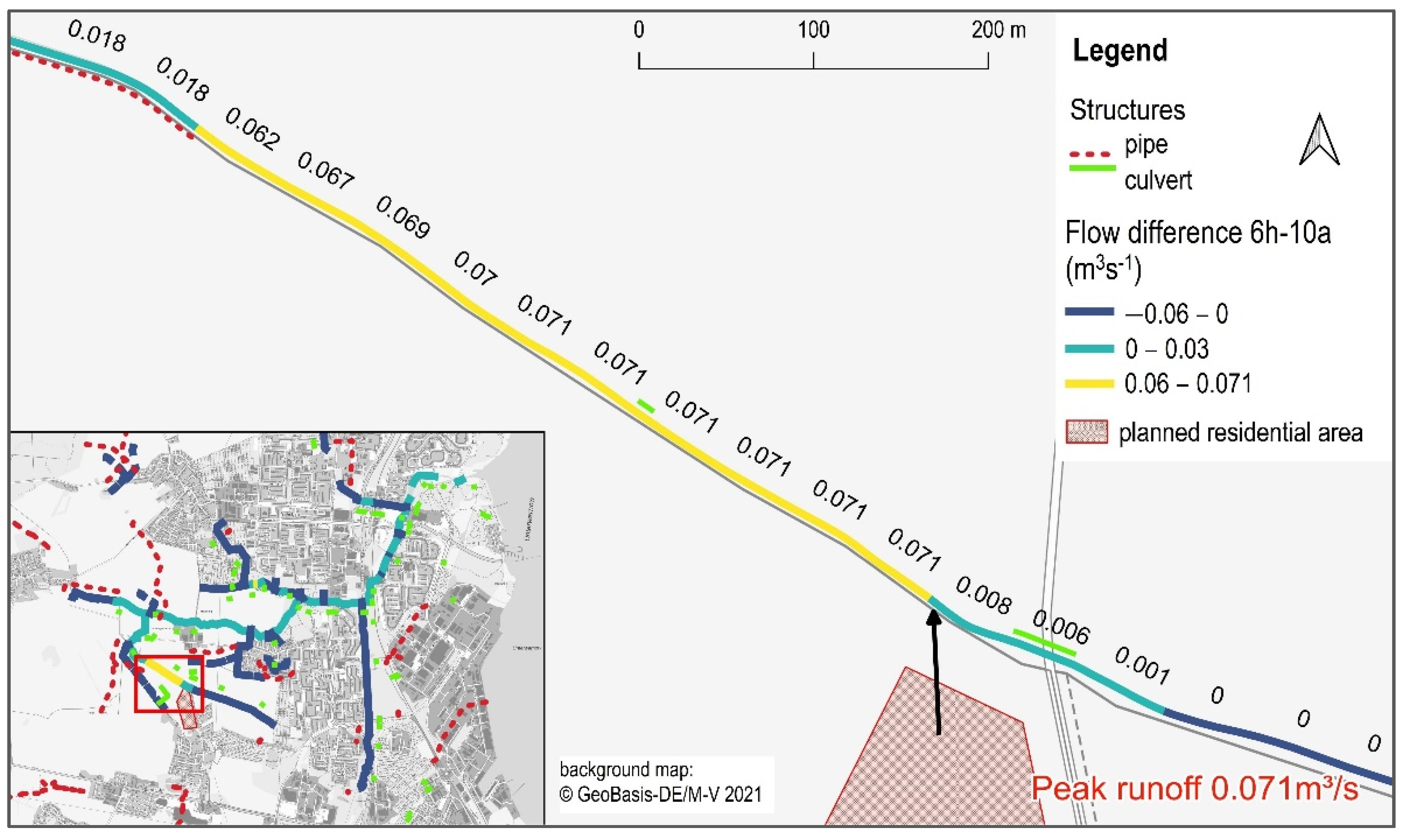
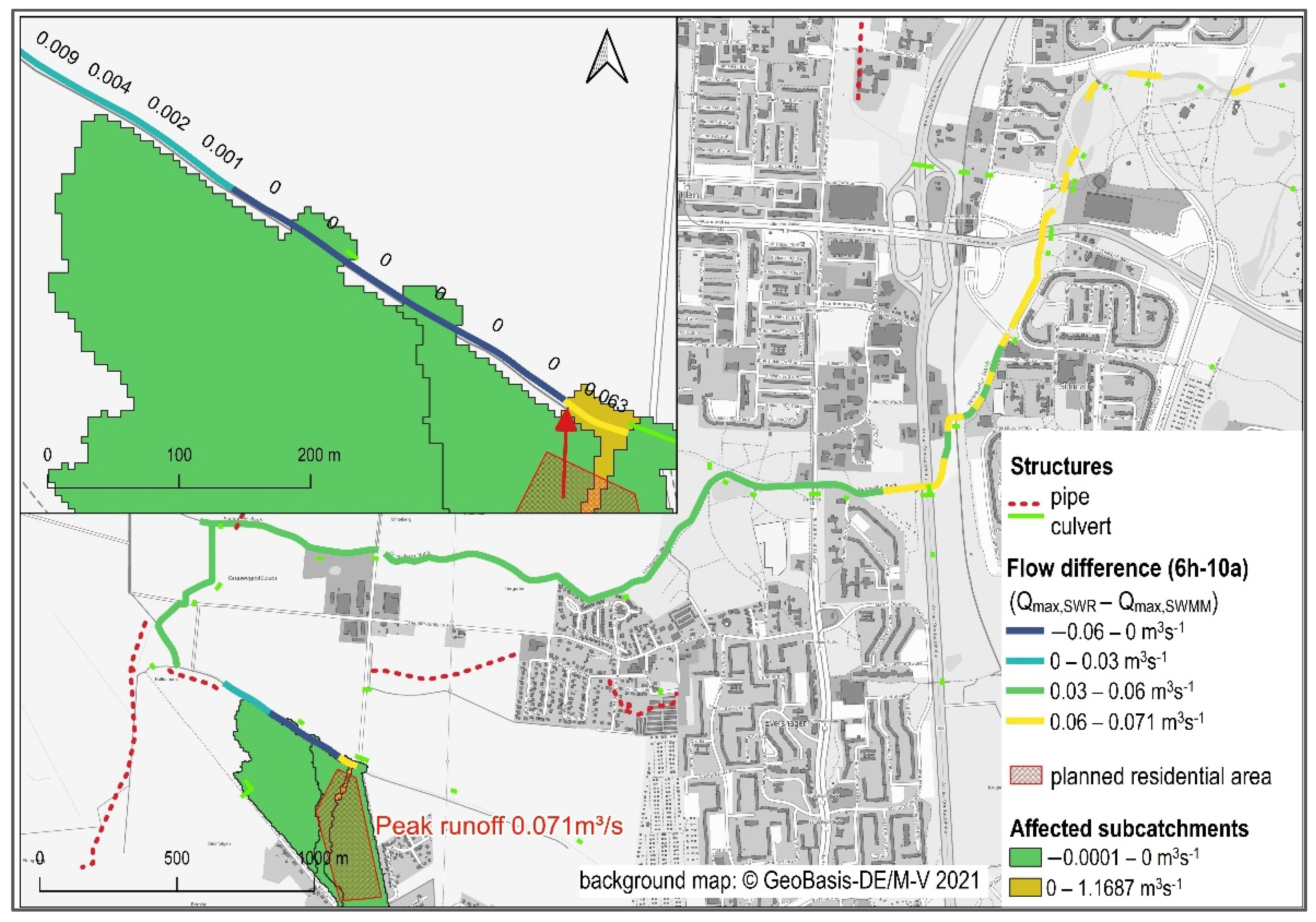
3.2.2. Comparison of Storm Water Routine Results with Model Results for the Plan State

Regarding peak runoff, the deviations of the results achieved by the SWR from those of the model tend to be larger the shorter the event is. As validation criterion, SWR results for events with a relative deviation smaller than 10% were classified as ‘good’. As shown in

Table 5. Comparison of the simulated (SWMM) and calculated (SWR) direct runoff of the planned residential area (70% sealed).

	Peak Runoff Simulated with SWMM (m3s−1)	Peak Runoff Calculated with SWR (m3s−1)	Runoff Difference (m3s−1)	Relative Deviation (%)
1 h–2 a	0.209	0.309	0.100	32
1 h–100 a	0.820	1.169	0.349	30
3 h–10 a	0.131	0.123	−0.008	−7
3 h–25 a	0.163	0.158	−0.005	−3
3 h–50 a	0.191	0.192	0.001	0
3 h–100 a	0.229	0.224	−0.005	−2
6 h–10 a	0.071	0.071	0.000	0
6 h–25 a	0.083	0.087	0.004	5
6 h–50 a	0.097	0.094	−0.004	−4
6 h–100 a	0.119	0.109	−0.009	−9
9 h–10 a	0.051	0.051	0.000	0
9 h–25 a	0.059	0.059	0.000	0
9 h–50 a	0.066	0.066	0.000	0
9 h–100 a	0.076	0.078	0.002	2
12 h–10 a	0.040	0.038	−0.001	−3
12 h–25 a	0.046	0.046	0.000	0
12 h–50 a	0.052	0.052	0.000	0
12 h–100 a	0.059	0.059	0.001	1

, this applies to all SWR peak runoffs with a duration of 3 h and longer which have a coefficient of determination higher than 0.9.

The two 1 h events, whose triggering rains show a varying intensity course, deviate considerably with 30% and 32%, respectively. It should be noted here that more accurate results for those events would have been expected if the degree of sealing for the planned area had been <50% (cf. correlation for 1 h events in Figure 6). However, the peak runoffs for the 1 h events calculated with SWR can be taken as the mean area response if other parameters (gradient, flow length, roughness, etc.) are still unknown in the process of planning.

Figure 12 illustrates the effect of the user-defined discharge point. The sealed residential area overlaps four subcatchments where in this precipitation scenario (6 h–10 a) hardly any runoff was generated in the initial state. In the planning scenario, the surface runoff increases by 0.071 m³s⁻¹ in the selected subcatchment (highlighted in yellow), while in the other three subcatchments the runoff slightly decreases or remains unchanged.

During more extreme events such as 1 h–100 a (Figure 13), runoff also occurs on the unsealed subcatchments in the initial state. As the planned area drains only into the central user-defined segment (+1.169 m³s⁻¹), the resulting difference in runoff of adjacent and intersected subcatchments is negative in the planning scenario (blue and green areas in Figure 13).

When comparing SWR-calculated peak flows with those simulated by SWMM the results directly downstream of the discharge point (300 m reach) are nearly identical (cf. Figure 12). With increasing distance, however, the differences become larger. This can be explained by different hydraulic effects such as wave flattening and retention in the hydraulic model, which are not implemented in the simplified routing algorithm of the SWR. The same applies for the deviations between SWR and model directly upstream of the discharge point. Due to backwater, a part of the runoff flows upstream for a short time in the model (cf. Figure 11), which the SWR does not take into account. After heavy rainfall events, the deviations of the peak flows can be even larger than the indicated runoff difference from Table 5, due to the flow redistribution (flow direction downstream and upstream), which the SWR cannot consider.

Additionally, the different spatial resolutions of both approaches have an impact here: In order to be consistent with other data sets of the DSS, the SWR routes the peak runoff from the discharge point along river sections of 50 m length. By contrast, the hydraulic model in SWMM uses river segments of varying length to address any relevant changes (profile, infrastructure).

Despite the mentioned simplifying approaches, the SWR enables a rapid evaluation of the impact of land use change scenarios on flood risk. Figure 14 shows an exemplary result for flow capacities (Q_{max, SWR}/Q_full * 100 %) calculated by the SWR for the 6 h–10 a event. The colors of the stream segments indicate how critical its water level could rise in the planning scenario. Pink sections mark the areas that could potentially be affected by flooding, especially if the capacity is greater than 100%.

4. Discussion

Before discussing the pros and cons of total approach, the background and overall objectives shall be shortly remembered: The developed approach shall enable regional planners, water authorities, and other stakeholders to assess the potential impact of planned land use changes on runoff, peak flow, and related flood risk in the receiving river system. Focus water bodies are small lowland rivers, often without any monitoring data for model calibration. The often missing modeling expertise of the stakeholders is addressed replacing detailed modeling by GIS based analysis.

Summarizing parts 1 [22] and 2 (this paper), the approach consists of two major steps:

• Setup and parametrization of a detailed hydrologic/hydrodynamic model
• Forecasting runoff change induced by land use changes and downstream flood risks applying newly developed GIS routines

For consistency, here, we shortly repeat the main findings of step 1. For the combined representation of rainfall-runoff and hydrodynamic streamflow processes, we selected the free-ware model SWMM-UrbanEVA. Since the model is physically based, it can be strictly setup and parametrized using geodata. We proposed an according workflow, including the definition of important model parameters, for lowland river basins. The approach was shown and tested for two river basins representing two extremes of approximately 20 superior catchments in the northeast German lowlands. Even though all are located in the same climatic and geo-morphologic zone, they differ in some characteristics (e.g., average terrain slope, depth to groundwater table, dominant land use, etc.). For the here interesting peak runoff, the most hydrologically significant attribute is land use, specifically the degree of urbanity or the percentage of sealed surfaces. It was found that the model performed better at stronger urbanised river basin. As discussed there, the lower model performance is only partly due to the parametrization but rather to uncertain rain data. Though, it can be postulated that the object data of urbanised areas are in most cases better documented and the rainfall-runoff process is less complex, leading to an expectable better model performance compared to near natural river basins. Despite the proposed strict and highly automated workflow based on geodata, model setup still requires an experienced modeler.

For the flood risk analysis, model based or with the GIS tool, distinct precipitation scenarios have to be chosen. Here, we propose synthetic rains, characterised by reoccurrence interval and duration. The reoccurrence intervals have to be chosen according to the desired protection level of the different land uses. The advantages of this approach are short computation time and the availability of regionalised rain data. However, the approach is very sensitive to the initial condition of the model, when precipitation starts. Here, we preprocessed the model using rain times series to produce average flow. More detailed analysis of rain statistics may lead to more differenced settings for the initial condition according to the precipitation scenario.

Once the model exists, the analysis of land use changes can be performed by any person with basic GIS skills. As the above discussed results show, the simplified calculation of runoff, based on the rain intensity dependent peak runoff functions matches very well with the results of the physical model. Since only a static peak runoff is applied, the calculation accuracy decreases with increasing impact of dynamics, as seen here for the 1 h precipitation scenario. The same applies for the routed stream runoff in river. For rain duration stages between 6 h to 12 h, the results of the benchmark model are met very well (R² > 096), while dynamic effects for short duration stages (wave flattening, backwater effects) cannot be addressed by the simplified routing algorithm. Generally, the routing tends to overestimate downstream flow effects and is, regarding the impact assessment, on the safe side.

The method presented here was specifically tailored to the study area and the available data, but if similar data sets are available, it is also very well transferable to other sites. It should be noted that the proposed peak runoff functions have been derived for the characteristics of rather flat morphology and short distances between regarded area and discharge point. In other regions or spatial conditions, the terrain gradient or the flow length may lead to deviating peak runoff coefficients. Case specific functions can be derived as described above.

A great advantage of the method is the evaluation of flood risk for planners without the setup of a complex model, as proposed by [12].

Compared to earlier approaches, assessing runoff induced by land us change in the past ([3,4]), the SWR can be applied to predict runoff from future settlement areas. Additionally, not only runoff, but the actual flood risk is assessed.

For this, the method goes in two dimensions one step further: i) small scale land use change can be directly allocated and assessed; ii) the spread of runoff in the watercourse is calculated by incorporating high resolution DEM-derived stream geometry and characteristics. Considering that the method is to be used primarily in early planning phases, when it is perhaps just known that an industrial area of a certain size is to be built in a district, for example, it is a great progress if the stream hydraulic impact can be calculated immediately without prior knowledge. The method quickly shows tendencies where the water is overflowing and where additional measures may be necessary.

Following the generic framework of [15], the tool can be regarded partly as collaborative and partly as participatory modeling approach. Arguments for real collaborative modeling are:

• The modeling concept has been developed jointly
• The data for the model are accessible for or provided by the decision-makers and stakeholders
• The tool is designed interactively and embedded in a familiar GIS environment
• Results are processed and visualized for direct use (interactive planning, decision on storm water discharge applications, etc.)

However, the underlying process models set up with SWMM-UrbanEVA will require regular updates (changes of assets, land-use). Still, this requires an expert modeler. Though the highly automated model setup strictly based on geodata (see part 1) simplifies model updates significantly, this task should remain in one hand to avoid inconsistent model versions at the various partners.

Currently, the tool provides one-dimensional information of flood risk. For experienced users, this is already highly informative. However, these data are less suitable for dissemination to citizens, since interpretation of an actual precise flood risk at a certain point would require well-considered 2D flood maps [17] and in best case a clear instruction, what a certain flood level means for the property and which response measures should be taken [30]. This applies even more, since information on flood risk have clear financial consequences for property owners [31]. Therefore, the main purpose of this tool is not to warn citizens, but to avoid flood risks by interactive sustainable land use planning and well-reasoned definition of tolerable storm water discharges.

In validating the results produced using the SWR tool, citizen science can be an important component (cf. [32,33]). For example, the tool shows us stream segments that potentially spill during heavy rain events. Interviewing eyewitnesses to past flooding events can help confirm potential problem areas. More automatable is the evaluation of social media comments on flooding events (e.g., Twitter) [34]. Therefore, the latter is particularly suitable for large-scale observations.

5. Conclusions and Outlook

This study presents a procedure that uses a simple method to calculate the impact of planned land use changes on river flow and potential flooding. It combines a detailed hydrologic and hydrodynamic model set up for the status quo with a simplified forecast of direct runoff in the planning scenario, which is routed through the downstream watercourse network.

The SWR forecast tool is easy and intuitive to use and does not necessarily demand modeling experience. It requires only the drawing or uploading of one or more new land use polygons, the planned degree of sealing and the precipitation scenario of interest. The calculations in the GIS-DSS take only few seconds, so that several scenarios can be tested and compared efficiently—e.g., size and location of area, degree of sealing or discharge point. The advanced visualization of the results, for example the display of overloaded river sections, improves communication with stakeholders enormously [33].

The underlying physically based process model can be set-up highly automated based on available geodata. For comparable catchment characteristics a parameter transfer from gauged to ungauged catchments is possible with tolerable loss of model accuracy.

Nevertheless, the described method is based on simplifications that may deviate more or less from reality. Three main sources of uncertainty can be mentioned here:

-

Uncertainty of the input data (object data, time series of rainfall and flow) for set-up and calibration/parametrization of the process model for the current state (in the investigated river basins the resulting peak runoff error was 8–26 %)

-

Inaccuracies in the simplified calculation of the peak runoff of a newly planned site: 0–32 % (depending on rain scenario)

-

Inaccuracies in the propagation of additional peak runoff in the watercourse: 0–1.07 m³s⁻¹ downstream of discharge point and 0.06–1.05 m³s⁻¹ upstream (depending on rain scenario)

A flood event is a transient process, whereas the applied calculation method is stationary. Therefore, the presented method performs better for block rains of larger durations. Generally, the deviations between SWR-calculated and simulated peak flows increase with distance from the discharge point downstream due to wave attenuation and flow retention. However, this is not to be seen as a shortcoming—rather, the calculated maximum flows represent the potential changes in planned state and thus have a warning effect on the user. In the exemplary case, downstream of the imaginary discharge point, an enlargement of the pipeline was discussed, which would reduce the retention effect and might produce flooding in the lower reach.

Although the results of the SWR already provide the user with a great deal of information gain, several suggestions for improvement can be derived.

The implementation of a retention factor per stream segment would be conceivable for the routing of peak flows. These could be calculated directly from the model results as a percentage of the respective upstream flow. It would also be possible and simple to implement to stop the routing as soon as the capacity is exceeded at a point in the watercourse (typically a culvert). However, this ‘improvement’ has to be taken with care since it cannot be ruled out that in reality the water continues to flow on the surface of the terrain and enters the stream again at another point.

As a next step, the intersection of the flooded stream segments with the surrounding land uses (and their required level of protection/return period) would also be conceivable, e.g., by means of a 50 m buffer around the segments. The land use polygons where the required level of protection cannot be achieved could subsequently be marked with a warning color.

What has not been addressed, yet, is the possibility of using the SWR tool for low impact design measures (LID) [35]. The required conceptual approach to link LID measures with direct runoff calculations could be derived from scenario modeling using SWMM-UrbanEVA. This upgrade of SWR would allow a fast preliminary design and allocation of LID to mitigate existing or potential flooding situations.

References

1. Poelmans, L.; van Rompaey, A.; Batelaan, O. Coupling urban expansion models and hydrological models: How important are spatial patterns? Land Use Policy 2010, 27, 965–975. [Google Scholar] [CrossRef]
2. Park, G.; Park, H. Influence analysis of land use by population growth on urban flood risk using system dynamics using system dynamics. In Environmental Impact IV, Proceedings of the Environmental Impact 2018, Naples, Italy, 20–22 June 2018; Casares, J., Passerini, G., Perillo, G., Eds.; WIT Press: Southampton, UK, 2018; pp. 195–205. [Google Scholar]
3. Shi, P.-J.; Yuan, Y.; Zheng, J.; Wang, J.-A.; Ge, Y.; Qiu, G.-Y. The effect of land use/cover change on surface runoff in Shenzhen region, China. CATENA 2007, 69, 31–35. [Google Scholar] [CrossRef]
4. Weng, Q. Modeling urban growth effects on surface runoff with the integration of remote sensing and GIS. Environ. Manag. 2001, 28, 737–748. [Google Scholar] [CrossRef]
5. Kind, J.; Wouter Botzen, W.J.; Aerts, J.C. Accounting for risk aversion, income distribution and social welfare in cost-benefit analysis for flood risk management. WIREs Clim. Chang. 2017, 8, e446. [Google Scholar] [CrossRef]
6. Alexakis, D.D.; Grillakis, M.G.; Koutroulis, A.G.; Agapiou, A.; Themistocleous, K.; Tsanis, I.K.; Michaelides, S.; Pashiardis, S.; Demetriou, C.; Aristeidou, K.; et al. GIS and remote sensing techniques for the assessment of land use change impact on flood hydrology: The case study of Yialias basin in Cyprus. Nat. Hazards Earth Syst. Sci. 2014, 14, 413–426. [Google Scholar] [CrossRef] [Green Version]
7. Deguid, K. Here’s What Flood Damage Is Predicted to Cost America by 2051. Available online: https://www.weforum.org/agenda/2021/02/cost-of-flood-damage-to-u-s-homes-will-increase-by-61-in-30-years/ (accessed on 19 July 2021).
8. Pitt, M. The Pitt ReviewLearning Lessons from the 2007 Floods. Available online: https://webarchive.nationalarchives.gov.uk/20100812084907/http://archive.cabinetoffice.gov.uk/pittreview/_/media/assets/www.cabinetoffice.gov.uk/flooding_review/pitt_review_full%20pdf.pdf (accessed on 2 February 2021).
9. Tsatsaris, A.; Kalogeropoulos, K.; Stathopoulos, N.; Louka, P.; Tsanakas, K.; Tsesmelis, D.E.; Krassanakis, V.; Petropoulos, G.P.; Pappas, V.; Chalkias, C. Geoinformation Technologies in Support of Environmental Hazards Monitoring under Climate Change: An Extensive Review. IJGI 2021, 10, 94. [Google Scholar] [CrossRef]
10. Mysiak, J.; Giupponi, C.; Rosato, P. Towards the development of a decision support system for water resource management. Environ. Model. Softw. 2005, 20, 203–214. [Google Scholar] [CrossRef]
11. Levy, J.K. Multiple criteria decision making and decision support systems for flood risk management. Stoch. Environ. Res. Risk Assess. 2005, 19, 438–447. [Google Scholar] [CrossRef]
12. Wang, L.; Cheng, Q. Design and implementation of a web-based spatial decision support system for flood forecasting and flood risk mapping. In Proceedings of the 2007 IEEE International Geoscience and Remote Sensing Symposium, Barcelona, Spain, 23–28 July 2007; IEEE: Piscataway, NJ, USA, 2007; pp. 4588–4591, ISBN 978-1-4244-1211-2. [Google Scholar]
13. Todini, E. An operational decision support system for flood risk mapping, forecasting and management. Urban Water 1999, 1, 131–143. [Google Scholar] [CrossRef]
14. Mahmoud, S.H.; Gan, T.Y. Urbanization and climate change implications in flood risk management: Developing an efficient decision support system for flood susceptibility mapping. Sci. Total Environ. 2018, 636, 152–167. [Google Scholar] [CrossRef] [PubMed]
15. Basco-Carrera, L.; Warren, A.; van Beek, E.; Jonoski, A.; Giardino, A. Collaborative modelling or participatory modelling? A framework for water resources management. Environ. Model. Softw. 2017, 91, 95–110. [Google Scholar] [CrossRef]
16. Maskrey, S.A.; Mount, N.J.; Thorne, C.R.; Dryden, I. Participatory modelling for stakeholder involvement in the development of flood risk management intervention options. Environ. Model. Softw. 2016, 82, 275–294. [Google Scholar] [CrossRef]
17. Luke, A.; Sanders, B.F.; Goodrich, K.A.; Feldman, D.L.; Boudreau, D.; Eguiarte, A.; Serrano, K.; Reyes, A.; Schubert, J.E.; AghaKouchak, A.; et al. Going beyond the flood insurance rate map: Insights from flood hazard map co-production. Nat. Hazards Earth Syst. Sci. 2018, 18, 1097–1120. [Google Scholar] [CrossRef] [Green Version]
18. Costabile, P.; Costanzo, C.; de Lorenzo, G.; de Santis, R.; Penna, N.; Macchione, F. Terrestrial and airborne laser scanning and 2-D modelling for 3-D flood hazard maps in urban areas: New opportunities and perspectives. Environ. Model. Softw. 2021, 135, 104889. [Google Scholar] [CrossRef]
19. Macchione, F.; Costabile, P.; Costanzo, C.; de Santis, R. Moving to 3-D flood hazard maps for enhancing risk communication. Environ. Model. Softw. 2019, 111, 510–522. [Google Scholar] [CrossRef]
20. Sanders, B.F.; Schubert, J.E.; Goodrich, K.A.; Houston, D.; Feldman, D.L.; Basolo, V.; Luke, A.; Boudreau, D.; Karlin, B.; Cheung, W.; et al. Collaborative Modeling With Fine-Resolution Data Enhances Flood Awareness, Minimizes Differences in Flood Perception, and Produces Actionable Flood Maps. Earth’s Future 2020, 7, e2019EF001391. [Google Scholar] [CrossRef] [Green Version]
21. Hoffmann, T.; Mehl, D.; Schilling, J.; Chen, S.; Tränckner, J.; Hinz, M.; Bill, R. GIS-basiertes Entscheidungsunterstützungssystem für die prospektive synergistische Planung von Entwicklungsoptionen in Regiopolen am Beispiel des Stadt-Umland-Raums Rostock. gis.Science 2021. Manuscript submitted for publication. [Google Scholar]
22. Kachholz, F.; Tränckner, J. A Model-Based Tool for Assessing the Impact of Land Use Change Scenarios on Flood Risk in Small-Scale River Systems—Part 1: Pre-Processing of Scenario Based Flood Characteristics for the Current State of Land Use. Hydrology 2021, 8, 102. [Google Scholar] [CrossRef]
23. Kunze, U. Die Geschichte der Hansestadt. Available online: https://www.rostock.de/kultur/historisches/geschichte-der-hansestadt.html (accessed on 11 May 2021).
24. Olaf. Rostock Wächst Langsamer als Erwartet: Die Tatsächliche Bevölkerungsentwicklung Liegt in Rostock Deutlich Unter der Prognose von 2016—Die Grünen Wollen Mehr Grünflächen Erhalten. Available online: https://www.rostock-heute.de/rostock-einwohnerzahl-bevoelkerungsprognose/105402 (accessed on 12 May 2021).
25. Wimes—Stadt- und Regionalentwicklung. Bevölkerungsprognose 2030 für den LK Rostock: Endfassung. 2017. Available online: http://213.254.33.168/landkreis/daten_fakten/Bevxlkerungsprognose_2030_LK_Rostock.pdf (accessed on 12 May 2021).
26. Chen, S.; Hoffmann, T.G.; Mehl, D. Digitale Gewässerkataster: Grundlage von system- und prozessorientierter Raumanalyse und -planung. RaumPlanung 2021, 211/2-2021, 44–51. [Google Scholar]
27. Überflutungsvorsorge—Kommunale Gemeinschaftsaufgabe und verteilte Zuständigkeiten. Wasser Abfall 2017, 34–38.
28. Junghänel, T.; Ertel, H.; Deutschländer, T. KOSTRA-DWD-2010R Deutscher Wetterdienst: Bericht zur Revision der Koordinierten Starkregenregionalisierung und -Auswertung des Deutschen Wetterdienstes in der Version 2010; Offenbach am Main. 2017. Available online: https://www.dwd.de/DE/leistungen/kostra_dwd_rasterwerte/download/bericht_revision_kostra_dwd_2010.pdf?__blob=publicationFile&v=6 (accessed on 7 July 2021).
29. DWA. Arbeitsblatt DWA-A 118. Hydraulische Bemessung und Nachweis von Entwässerungssystemen; DWA: Hennef, Germany, 2006; ISBN 3939057150. [Google Scholar]
30. Rollason, E.; Bracken, L.J.; Hardy, R.J.; Large, A.R.G. Rethinking flood risk communication. Nat. Hazards 2018, 92, 1665–1686. [Google Scholar] [CrossRef] [Green Version]
31. Pilla, F.; Gharbia, S.S.; Lyons, R. How do households perceive flood-risk? The impact of flooding on the cost of accommodation in Dublin, Ireland. Sci. Total Environ. 2019, 650, 144–154. [Google Scholar] [CrossRef]
32. Sy, B.; Frischknecht, C.; Dao, H.; Consuegra, D.; Giuliani, G. Flood hazard assessment and the role of citizen science. J. Flood Risk Manag. 2019, 12, e12519. [Google Scholar] [CrossRef]
33. Voinov, A.; Kolagani, N.; McCall, M.K.; Glynn, P.D.; Kragt, M.E.; Ostermann, F.O.; Pierce, S.A.; Ramu, P. Modelling with stakeholders—Next generation. Environ. Model. Softw. 2016, 77, 196–220. [Google Scholar] [CrossRef]
34. Vettermann, F.; Weinzierl, T.; Bill, R. Monitoring Twitter Messages for Spatio-Temporal and Thematic Analysis—Twittermonitor Rostock. gis.Science 2018, 1/2018, 1–9. [Google Scholar]
35. Eckart, K.; McPhee, Z.; Bolisetti, T. Multiobjective optimization of low impact development stormwater controls. J. Hydrol. 2018, 562, 564–576. [Google Scholar] [CrossRef]
Figure 1. Relevant surface catchments of the study area and administrative boundaries.
Hydrology 08 00130 g001
Figure 2. (a) Land use (generalized); (b) watercourses consisting of open channels, pipes and culverts; (c) catchments with first three digits of hierarchical ID (colors are chosen at random); and (d) free profile capacities (m3s−1) at the example of the rain event 3 h–100 a.
Hydrology 08 00130 g002aHydrology 08 00130 g002b
Figure 3. Determination of flood characteristics for the planned state of land use using GIS-DSS tools.
Hydrology 08 00130 g003
Figure 4. Allocation of the runoff difference to the 50 m-stream segments without (a) or with (b) definition of a receiving segment (black box with red outline = throttle).
Hydrology 08 00130 g004
Figure 5. Schmarler Bach area with land use of the actual state. (a) Outline map, (b) complete Schmarler Bach catchment with the exemplary planned residential area in the central south (yellow box), (c) detail section of the planned residential area.
Hydrology 08 00130 g005
Figure 6. Correlation diagrams based on peak runoff coefficients and the degree of sealing (subheadings are composed of rainfall duration and return period).
Hydrology 08 00130 g006
Figure 7. Difference of flows (m3s−1) in planned and current state for the rain event 6 h–10 a simulated with SWMM (pipes and culverts are plotted with offset to original route).
Hydrology 08 00130 g007
Figure 8. Flow difference (m3s−1) in the immediate area of the discharge point for the rain event 6 h–10 a (pipes and culverts are plotted with offset to original route).
Hydrology 08 00130 g008
Figure 9. Flow difference (m3s−1) in the immediate area of the discharge point for the rain event 1 h–100 a simulated with SWMM.
Hydrology 08 00130 g009
Figure 10. Maximum capacity and ponded volume in the immediate area of the discharge point for the rain event 1 h–100 a (plan state).
Hydrology 08 00130 g010
Figure 11. Runoff from plan area and simulated stream flow with rain event 1 h–100 a in the conduit directly downstream (max. flow = 0.42 m3s−1) and upstream (min. flow = −0.264 m3s−1) of the discharge point from the new residential site.
Hydrology 08 00130 g011
Figure 12. Peak runoff generated on the affected subcatchments and flow difference in m3s−1 (Qmax,SWR − Qmax, SWMM) in plan state for the rain event 6 h–10 a.
Hydrology 08 00130 g012
Figure 13. Peak runoff generated on the affected subcatchments and flow difference in m3s−1 (Qmax,SWR − Qmax, SWMM) in plan state for the rain event 1 h–100 a.
Hydrology 08 00130 g013
Figure 14. Stream capacity in plan state calculated with the storm water routine for the rain event 6 h–10 a.
Hydrology 08 00130 g014