
Spatiotemporal Analysis of Available Freshwater Resources in Watersheds Across Northern New Jersey

Abstract
1. Introduction
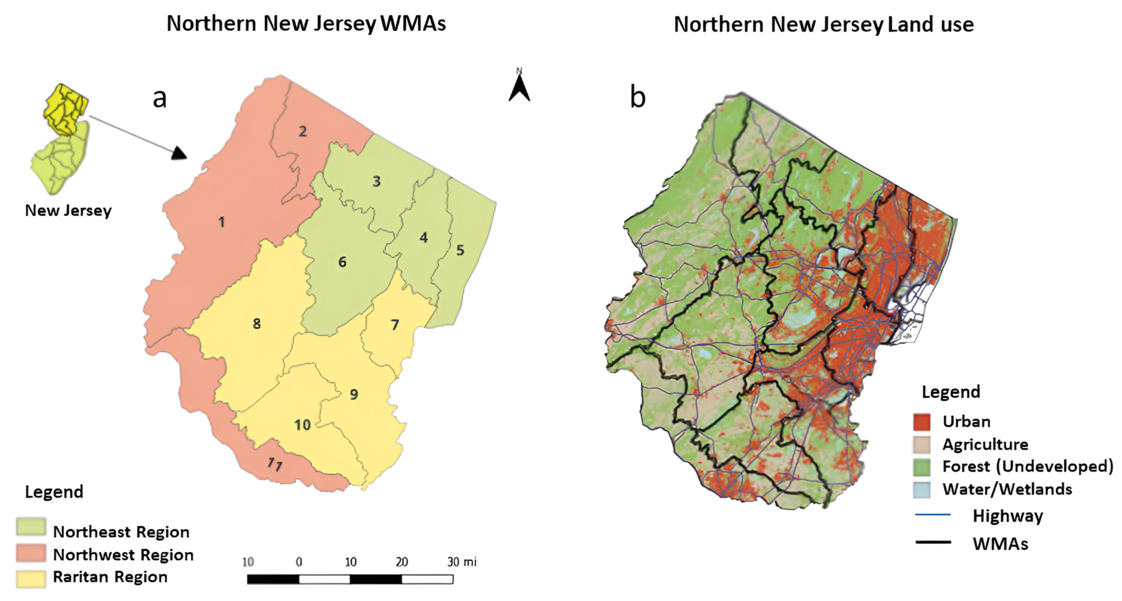
Study Area
2. Methods
2.1. Data Collection
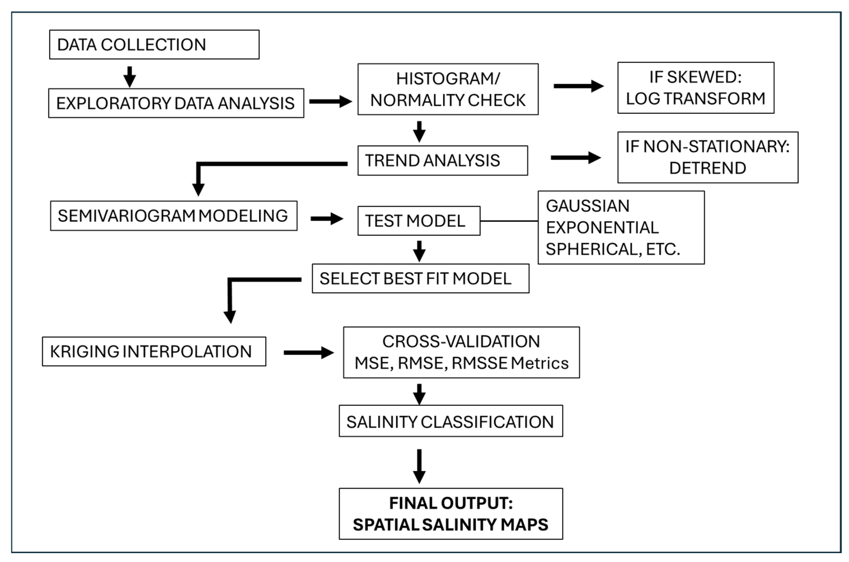
2.2. Data Analysis
2.2.1. Kriging Interpolation
2.2.2. Exploratory Data Analysis
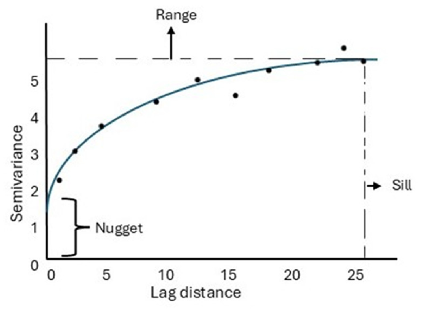
2.2.3. Experimental Semivariogram
2.2.4. Cross-Validation
2.2.5. Kriging Map Generation
2.2.6. Limitation
3. Results and Discussion
3.1. Exploratory Data Analysis
3.2. Experimental Semi-Variogram
3.3. Cross-Validation
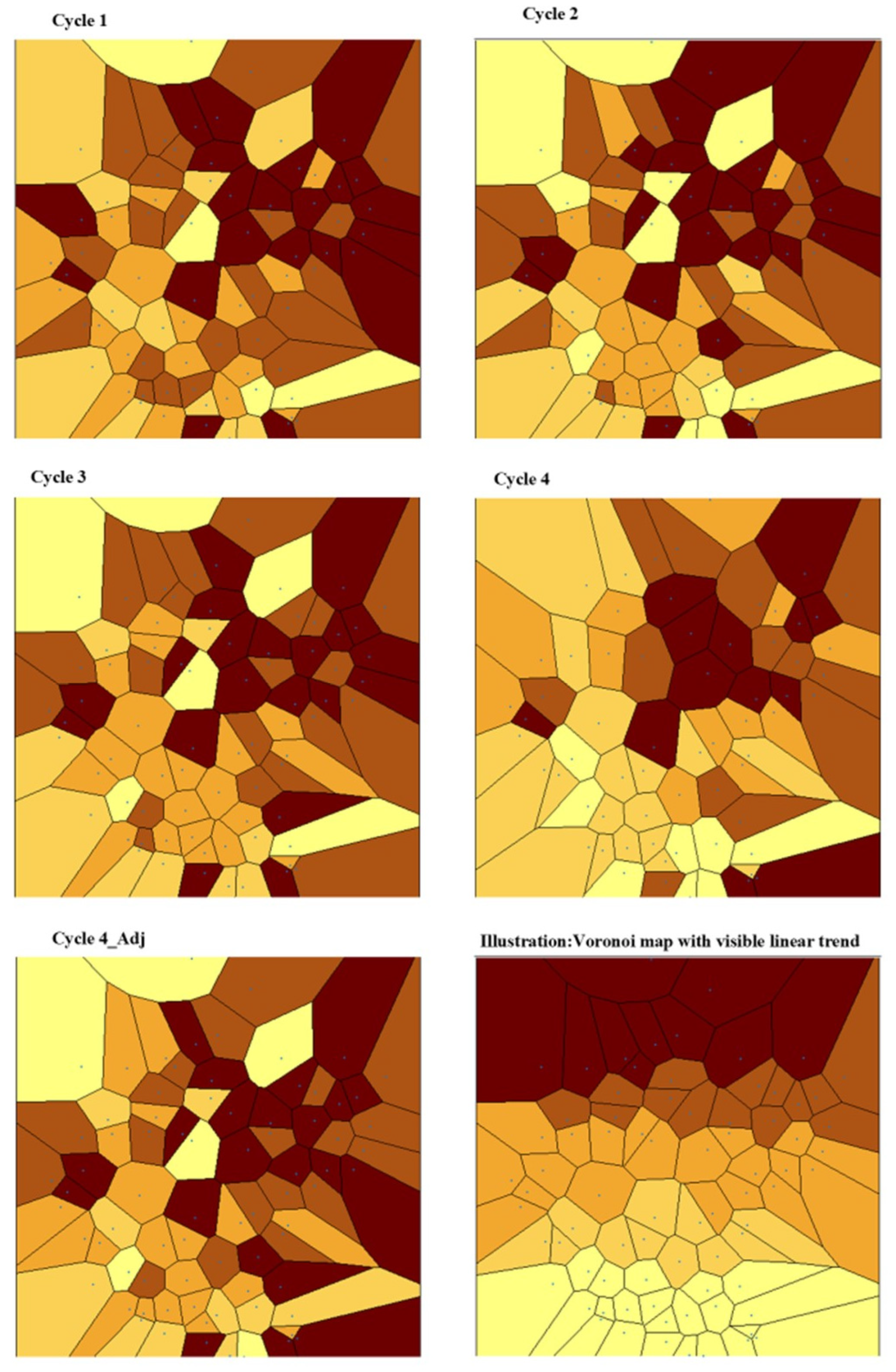
3.4. Kriging Map Generation
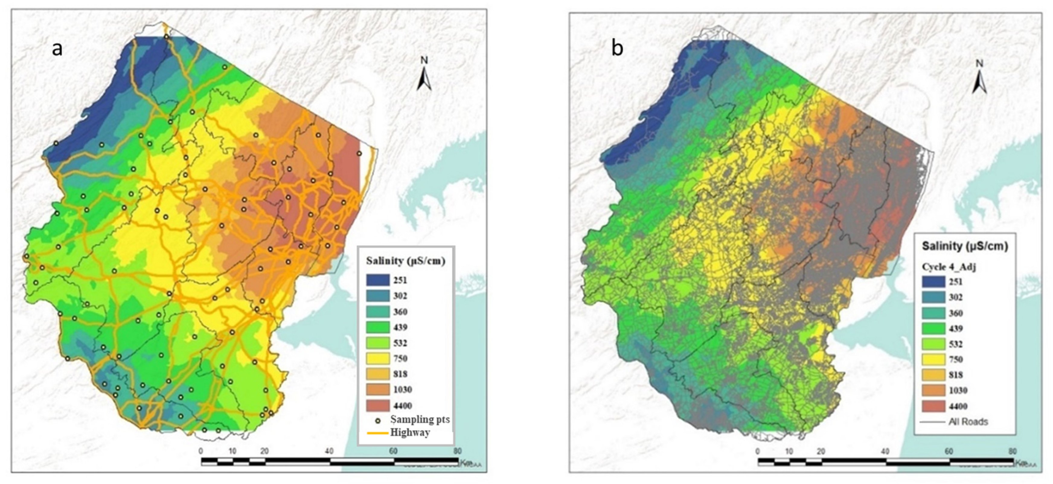
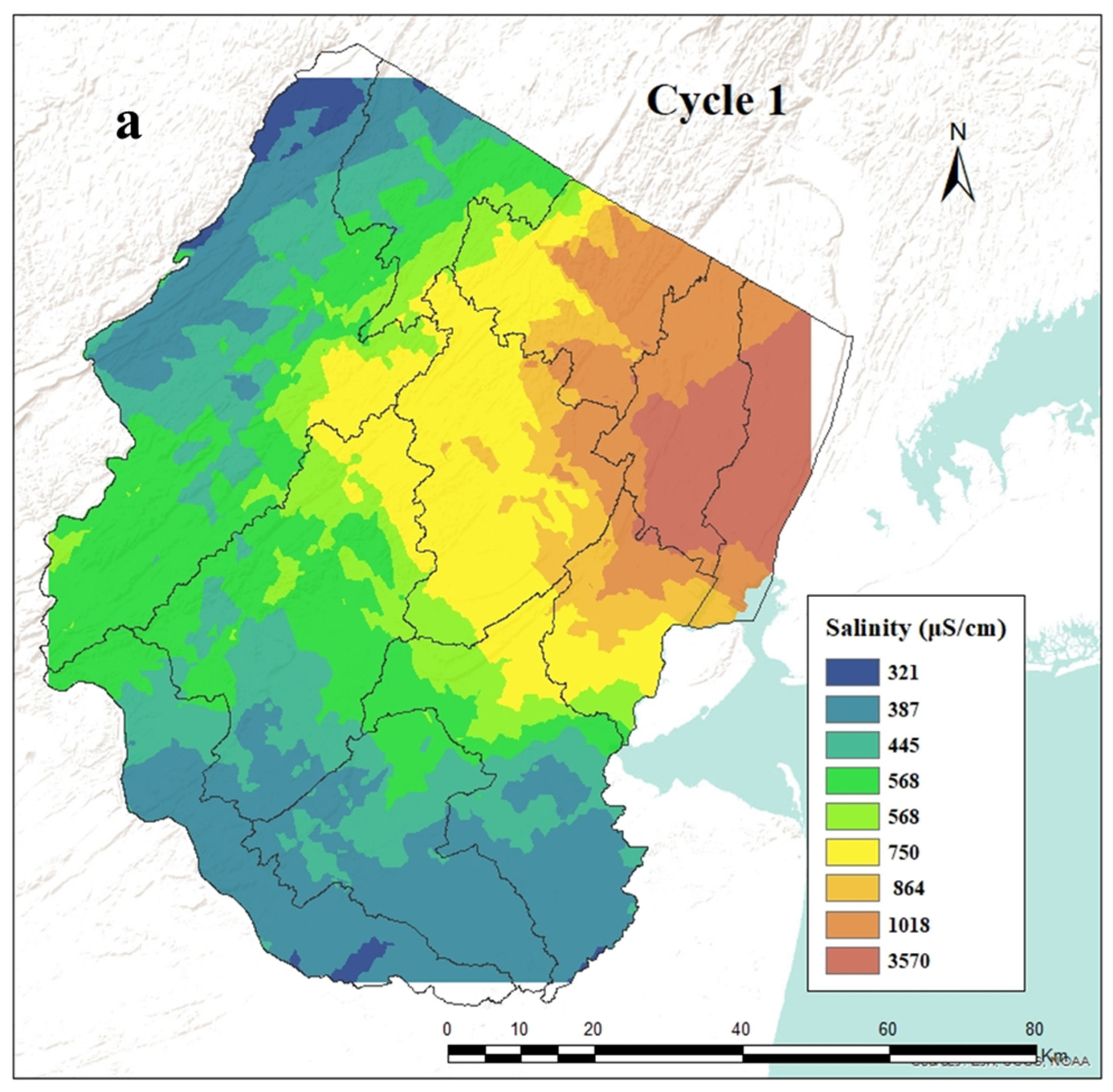
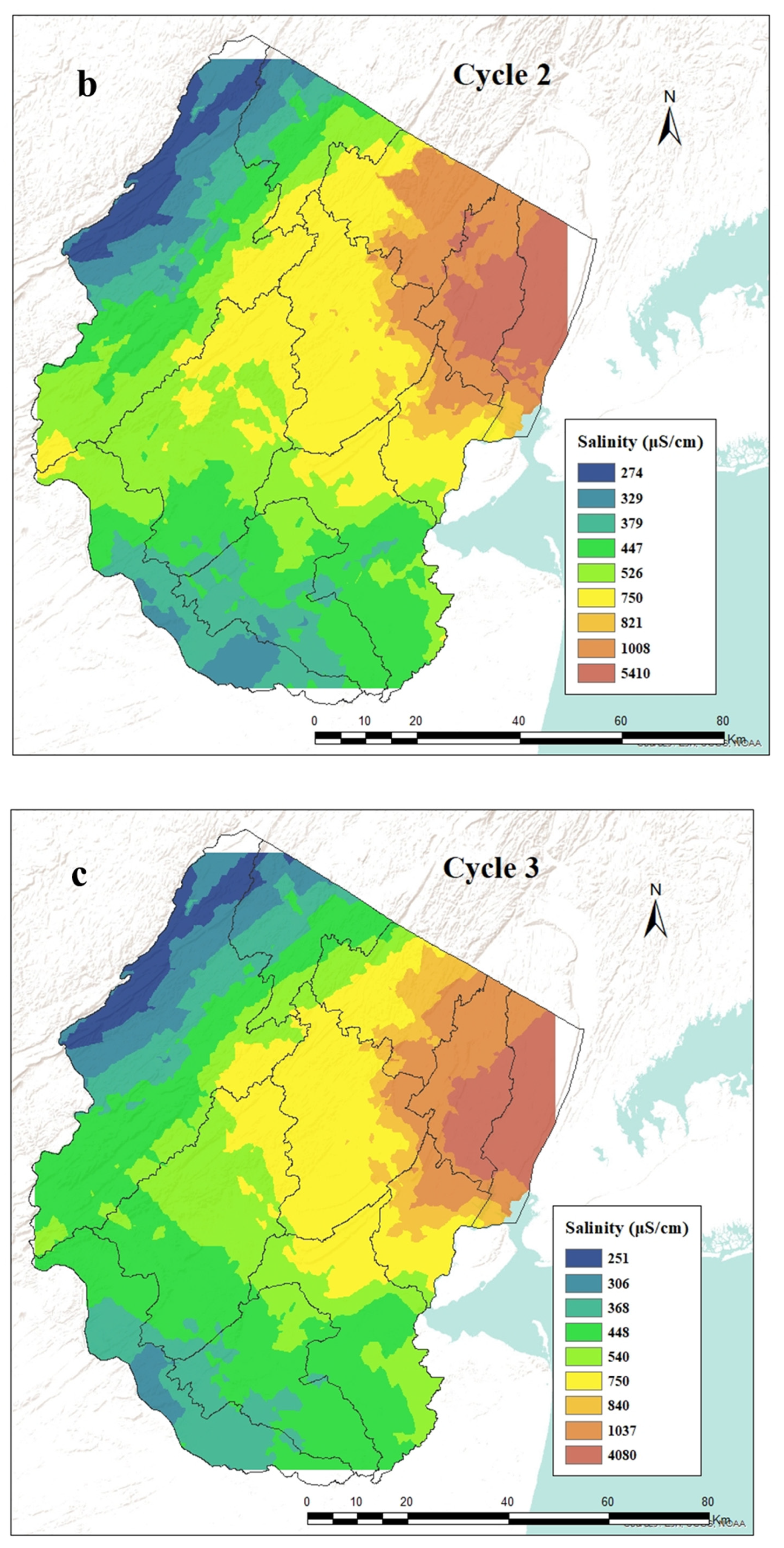
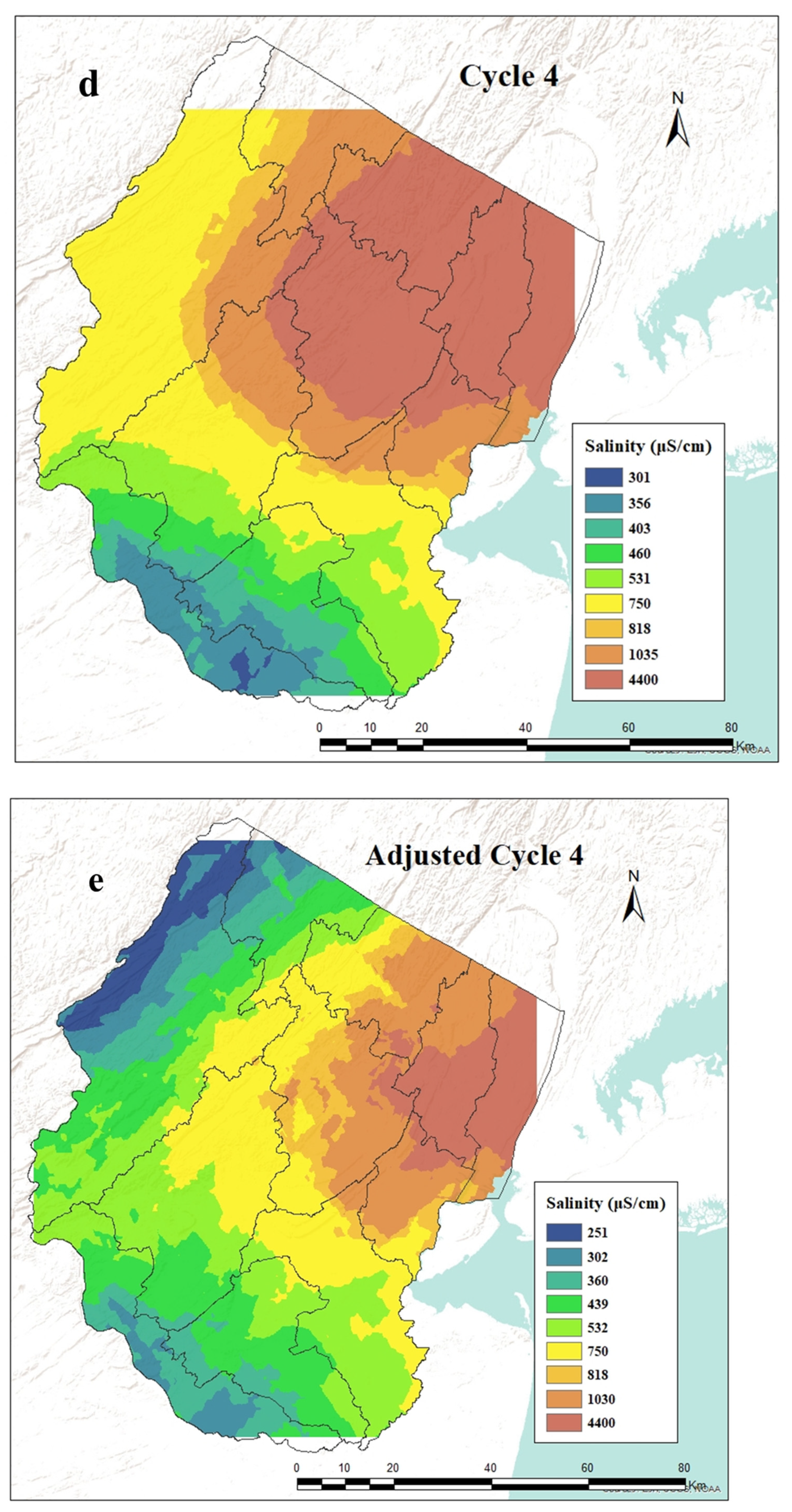
3.4.1. Groundwater Salinization Patterns in Northern New Jersey
- Northeast region: Persistent hotspots (WMAs 4–5) correlated not only with road density and NJDOT salt application rates (10,000 kg/lane-km [16]) but also with the highest urbanization intensity in the study area. Over 23% of this region transitioned towards urban land use between 1995 and 2000 [28], increasing impervious surfaces and concentrating deicing salt inputs.
- Northwest region: Lower specific conductance (<500 μS/cm) reflected the area’s agricultural and forested land uses, which typically experience reduced salinity inputs [8]. However, localized spikes in Cycles 2–3 suggest occasional fertilizer inputs, highlighting how agricultural land use can contribute to non-point source salinity.
- Raritan region: Emerging salinity increases in “adjusted Cycle 4” aligned with suburban expansion, where aging septic systems and fragmented land cover may facilitate subsurface contaminant transport.
- Urban WMAs (4–7) showed salinity increases faster than agricultural areas, paralleling Lathrop [28]’s documented land use shifts in New Jersey.
- Forested areas (e.g., Pompton WMA) retained stable freshwater coverage, highlighting the protective role of undeveloped land.
3.4.2. Integrated Drivers of Freshwater Decline and Management Implications
- Targeted salt reduction in WMA4–5, where road networks intersect vulnerable freshwater resources
- Enhanced monitoring networks, particularly in forested transition zones of WMA3, where the current well density underestimates salt accumulation
- Adaptive threshold management, including a biennial review of the 750 μS/cm benchmark to account for accelerating salinization trends particularly in the Northeast region
4. Conclusions
Supplementary Materials
Author Contributions
Funding
Data Availability Statement
Conflicts of Interest
References
- Dieter, C.A.; Maupin, M.A.; Caldwell, R.R.; Harris, M.A.; Ivahnenko, T.I.; Lovelace, J.K.; Barber, N.L.; Linsey, K.S. Estimated use of water in the United States in 2015. U.S. Geol. Surv. Circ. 2018, 1441, 65. [Google Scholar] [CrossRef]
- Khan, M.; Almazah, M.M.A.; EIlahi, A.; Niaz, R.; Al-Rezami, A.Y.; Zaman, B. Spatial interpolation of water quality index based on Ordinary kriging and Universal kriging. Geomat. Nat. Hazards Risk 2023, 14, 2190853. [Google Scholar] [CrossRef]
- Maupin, M.A.; Kenny, J.F.; Hutson, S.S.; Lovelace, J.K.; Barber, N.L.; Linsey, K.S. Estimated use of water in the United States in 2010. U.S. Geological Survey Circular 2014, 1405, 56. [Google Scholar] [CrossRef]
- Reilly, T.E.; Dennehy, K.F.; Alley, W.M.; Cunningham, W.L. Ground-Water Availability in the United States. U.S. Geol. Surv. Circ. 2008, 1323, 70. Available online: https://pubs.usgs.gov/circ/1323/pdf/Circular1323_book_508.pdf (accessed on 31 May 2023).
- Pace, M.L.; Bailey, N.W.; Utz, R.M.; Halevi, S.; Duan, S.; Kaushal, S.S.; Wessel, B.M.; Wood, K.L.; Maas, C.M.; Galella, J.G.; et al. Freshwater salinization syndrome: From emerging global problem to managing risks. Biogeochemistry 2021, 154, 255–292. [Google Scholar] [CrossRef]
- Sathe, S.S.; Mahanta, C. Groundwater flow and arsenic contamination transport modeling for a multi aquifer terrain: Assessment and mitigation strategies. J. Environ. Manag. 2019, 231, 166–181. [Google Scholar] [CrossRef]
- Serfes, M.; Bousenberry, R.; Gibs, J. New Jersey Ambient Ground Water Quality Monitoring Network: Status of shallow ground-water quality, 1999–2004. NJ Geol. Surv. Inf. Circ. 2007. Available online: https://www.nrc.gov/docs/ML1408/ML14086A280.pdf (accessed on 11 December 2019).
- Lindsey, B.D.; Fleming, B.J.; Goodling, P.J.; Dondero, A.M. Thirty years of regional groundwater-quality trend studies in the United States: Major findings and lessons learned. J. Hydrol. 2023, 627, 130427. [Google Scholar] [CrossRef]
- US Geological Survey. Groundwater Quality. U.S. Geological Survey Water Science School. 2025. Available online: https://www.usgs.gov/special-topics/water-science-school/science/groundwater-quality (accessed on 20 April 2023).
- Likens, G.E.; Band, L.E.; Belt, K.T.; Fisher, G.T.; Stack, W.P.; Kaushal, S.S.; Groffman, P.M.; Kelly, V.R. Increased salinization of fresh water in the northeastern United States. Proc. Natl. Acad. Sci. USA 2005, 102, 13517–13520. [Google Scholar] [CrossRef]
- Novotny, E.V.; Sander, A.R.; Mohseni, O.; Stefan, H.G. Chloride ion transport and mass balance in a metropolitan area using road salt. Water Resour. Res. 2009, 45, 12. [Google Scholar] [CrossRef]
- Ophori, D.; Firor, C.; Soriano, P. Impact of road deicing salts on the Upper Passaic River Basin, New Jersey: A geochemical analysis of the major ions in groundwater. Environ. Earth Sci. 2019, 78, 500. [Google Scholar] [CrossRef]
- Novotny, V.; Muehring, D.; Zitomer, D.H.; Smith, D.W.; Facey, R. Cyanide and metal pollution by urban snowmelt: Impact of deicing compounds. Water Sci. Technol. 1998, 38, 223–230. [Google Scholar] [CrossRef]
- Sarkar, D. Preliminary studies on mercury solubility in the presence of iron oxide phases using static headspace analysis. Environ. Geosci. 2003, 10, 151–155. [Google Scholar] [CrossRef]
- Bolen, W.P. Mineral Commodity Summaries; U.S. Geological Survey: Reston, VA, USA, 2020.
- New Jersey Department of Transportation (NJDOT). Winter Readiness, Expenditures, About NJDOT; NJDOT: Trenton, NJ, USA, 2018. Available online: https://www.nj.gov/transportation/about/winter/expenditures.shtm (accessed on 11 December 2019).
- NJDOT. New Jersey’s Roadway Mileage and Daily VMT by Functional Classification Distributed by County; NJDOT: Trenton, NJ, USA, 2020. Available online: https://www.nj.gov/transportation/refdata/roadway/pdf/hpms2019/VMTFCC_19.pdf (accessed on 11 December 2019).
- Harwell, M.C.; Surratt, D.D.; Barone, D.M.; Aumen, N.G. Conductivity as a tracer of agricultural and urban runoff to delineate water quality impacts in the northern Everglades. Environ. Monit Assess 2008, 147, 445–462. [Google Scholar] [CrossRef]
- Hems, J.D. Study Interpretation of the Chemical Characteristics of Natural Water, 3rd ed.; U.S. Geological Survey Water-Supply Paper; U.S. Geological Survey: Reston, VA, USA, 1985. Available online: https://pubs.usgs.gov/wsp/wsp2254/pdf/wsp2254a.pdf (accessed on 11 December 2019).
- McCleskey, R.B. New method for electrical conductivity temperature compensation. Environ. Sci. Technol. 2013, 47, 9874–9881. [Google Scholar] [CrossRef]
- US Geological Survey. Specific Conductance: U.S. Geological Survey Techniques and Methods, Book 9, Chap. A6.3; U.S. Geological Survey: Reston, VA, USA, 2019. [CrossRef]
- Cartwright, I.; Gilfedder, B.; Hofmann, H. Contrasts between estimates of baseflow help discern multiple sources of water contributing to rivers. Hydrol. Earth Syst. Sci. 2014, 18, 15–30. [Google Scholar] [CrossRef]
- Clean Water Team (CWT). Electrical conductivity/salinity Fact Sheet, FS-3.1.3.0(EC). In The Clean Water Team Guidance Compendium for Watershed Monitoring and Assessment; California State Water Resources Control Board: Sacramento, CA, USA, 2004. [Google Scholar]
- Balachandar, D.; Sundararaj, P.; Murthy, K.; Kumaraswamy, K. An Investigation of Groundwater Quality and Its Suitability to Irrigated Agriculture in Coimbatore District, Tamil Nadu, India—A GIS Approach. Int. J. Environ. Sci. 2010, 1, 176–190. [Google Scholar]
- US EPA. 5.9 Conductivity | Monitoring & Assessment; US EPA: Washington, DC, USA, 2012. Available online: https://archive.epa.gov/water/archive/web/html/vms59.html (accessed on 20 April 2023).
- United States Salinity Laboratory Staff (USSL). Diagnosis and Improvement of Saline and Alkaline Soils. Soil Sci. Soc. Am. J. 1954, 18, 348. [Google Scholar] [CrossRef]
- Raritan Basin Watershed Management Project. Raritan Basin: Portrait of a Watershed; New Jersey Water Supply Authority—Watershed Protection Programs; New Jersey Water Supply Authority: Clinton Township, NJ, USA, 2002; Available online: https://rucore.libraries.rutgers.edu/rutgers-lib/17036/ (accessed on 11 May 2022).
- Lathrop, R.G. Measuring Land Use Change in New Jersey: Land Use Update to Year 2000, A Report on Recent Development Patterns 1995 to 2000; Grant F. Walton Center for Remote Sensing & Spatial Analysis (CRSSA): New Brunswick, NJ, USA, 2004; 17-2004-1; Available online: https://crssa.rutgers.edu/projects/lc/docs/landuse_upd.pdf (accessed on 11 May 2022).
- Jalan, S.; Chouhan, D.S.; Chaure, S. Geospatial Analysis of Spatial Variability of Groundwater Quality Using Ordinary Kriging: A Case Study of Dungarpur Tehsil, Rajasthan, India. J. Geomat. 2022, 16, 176–187. [Google Scholar] [CrossRef]
- Watt, M.K. A Hydrologic Primer for New Jersey Watershed Management; USGS Water-Resources Investigations Report: West Trenton, NJ, USA, 2000. Available online: https://pubs.usgs.gov/wri/2000/4140/report.pdf (accessed on 11 December 2019).
- Arslan, H. Spatial and temporal mapping of groundwater salinity using ordinary kriging and indicator kriging: The case of Bafra Plain, Turkey. Agric. Water Manag. 2012, 113, 57–63. [Google Scholar] [CrossRef]
- Belkhiri, L.; Tiri, A.; Mouni, L. Spatial distribution of the groundwater quality using kriging and Co-kriging interpolations. Groundw. Sustain. Dev. 2020, 11, 100473. [Google Scholar] [CrossRef]
- Elubid, B.A.; Ahmed, E.H.; Zhao, J.; Elhag, K.M.; Abbass, W.; Babiker, M.M. Geospatial Distributions of Groundwater Quality in Gedaref State Using Geographic Information System (GIS) and Drinking Water Quality Index (DWQI). Int. J. Environ. Res. Public Health 2019, 16, 731. [Google Scholar] [CrossRef]
- Gharbia, A.S.; Gharbia, S.S.; Abushbak, T.; Wafi, H.; Aish, A.; Zelenakova, M.; Pilla, F. Groundwater Quality Evaluation Using GIS Based Geostatistical Algorithms. J. Geosci. Environ. Prot. 2016, 4, 89–103. [Google Scholar] [CrossRef]
- Johnson, C.D.; Nandi, A.; Joyner, T.A.; Luffman, I. Iron and Manganese in Groundwater: Using Kriging and GIS to Locate High Concentrations in Buncombe County, North Carolina. Groundwater 2018, 56, 87–95. [Google Scholar] [CrossRef]
- Li, J.; Heap, A.D.; Potter, A.; Huang, Z.; Daniell, J.J. Can we improve the spatial predictions of seabed sediments? A case study of spatial interpolation of mud content across the southwest Australian margin. Cont. Shelf Res. 2011, 31, 1365–1376. [Google Scholar] [CrossRef]
- Van Beers, W.C.M.; Kleijnen, J.P.C. Kriging Interpolation in Simulation: A Survey. In Proceedings of the 2004 Winter Simulation Conference, Washington, DC, USA, 5–8 December 2004; Ingalls, R.G., Rossetti, M.D., Smith, J.S., Peters, B.A., Eds.; 2004. Available online: https://informs-sim.org/wsc04papers/014.pdf (accessed on 31 May 2023).
- Tyagi, A.; Singh, P. Applying Kriging Approach on Pollution Data Using GIS Software. Int. J. Environ. Eng. Manag. 2013, 4, 185–190. Available online: http://www.ripublication.com/ijeem.htm (accessed on 31 May 2023).
- Siska, P.P.; Hung, I. Assessment of Kriging Accuracy in the GIS Environment. In Proceedings of the 21st Annual ESRI International User Conference, San Diego, CA, USA, 9–13 July 2001. Available online: https://proceedings.esri.com/library/userconf/proc01/professional/papers/pap280/p280.htm (accessed on 31 May 2023).
- Royle, J.A.; Nichols, J.D. Estimating Abundance from Repeated Presence-Absence Data or Point Counts—Tulane University. Ecology 2003, 84, 777–790. Available online: https://library.search.tulane.edu/discovery/fulldisplay?docid=cdi_proquest_miscellaneous_18770213&context=PC&vid=01TUL_INST:Tulane&lang=en&search_scope=MyInst_and_CI&adaptor=Primo%20Central&query=null,,PDF,AND&facet=citing,exact,cdi_FETCH-LOGICAL-c2640-4cc3ab70d55b63c5a41a56af47e37e4d20dae7847301f73cc0489de23a2d78ec3&offset=2 (accessed on 31 May 2023). [CrossRef]
- New Jersey Department of Environmental Protection. New Jersey’s Watersheds, Watershed management Areas and Water Regions; NJDEP Division of Watershed Management: Trenton, NJ, USA, 1997. Available online: https://dep.nj.gov/earthday/timeline/m1997/ (accessed on 11 December 2019).
- Dalton, R.F.; Monteverde, D.H.; Sugarman, P.J.; Volkert, R.A. Bedrock Geologic Map of New Jersey; New Jersey Geological Survey: Trenton, NJ, USA, 2014. Available online: https://www.nj.gov/dep/njgs/pricelst/Bedrock250.pdf (accessed on 11 December 2019).
- Drake, A.A.; Volkert, R.A., Jr.; Monteverde, D.H.; Herman, G.C.; Houghton, H.F.; Parker, R.A.; Dalton, R.F. Bedrock geologic map of northern New Jersey; U.S. Geological Survey: Reston, VA, USA, 1997. [CrossRef]
- New Jersey Department of Environmental Protection. Bedrock Geologic Map of New Jersey and Bedrock Geology of New Jersey; NJDEP—New Jersey Geological and Water Survey—U.S. Geological Survey: Reston, VA, USA, 2016. Available online: https://www.nj.gov/dep/njgs/enviroed/freedwn/psnjmap.pdf (accessed on 11 December 2019).
- Dalton, R. Physiographic Provinces of New Jersey; New Jersey Geological Survey Informational Circular; New Jersey Geological Survey: Trenton, NJ, USA, 2003. Available online: https://www.nj.gov/dep/njgs/enviroed/infocirc/provinces.pdf (accessed on 11 December 2019).
- Bousenberry, R. New Jersey Ambient Ground Water Quality Monitoring Network: New Jersey Shallow Ground-Water Quality, 1999–2008; New Jersey Geological and Water Survey Information Circular; New Jersey Geological Survey: Trenton, NJ, USA, 2016. Available online: https://www.nj.gov/dep/njgs/enviroed/infocirc/NJAGWQMN.pdf (accessed on 11 December 2019).
- R–Core Team. R: A Language and Environment for Statistical Computing; R Foundation for Statistical Computing: Vienna, Austria, 2023. [Google Scholar]
- QGIS.org. QGIS Geographic Information System; Open-Source Geospatial Foundation Project, n.d. Available online: https://qgis.org/ (accessed on 11 May 2020).
- ESRI. ArcGIS Pro: Understanding How to Remove Trends from the Data; ESRI–ArcGIS n.d. Available online: https://pro.arcgis.com/en/pro-app/latest/help/analysis/geostatistical-analyst/understanding-how-to-remove-trends-from-the-data.htm (accessed on 31 May 2023).
- Almodaresi, S.A.; Mohammadrezaei, M.; Dolatabadi, M. Qualitative Analysis of Groundwater Quality Indicators Based on Schuler and Wilcox Diagrams: IDW and Kriging Models. J. Environ. Health Sustain. Dev. 2019, 4, 903–915. [Google Scholar] [CrossRef]
- Boudibi, S.; Sakaa, B.; Zapata-Sierra, A.J. Groundwater Quality Assessment Using GIS, Ordinary Kriging and WQI in an Arid Area. PONTE Int. Sci. Res. J. 2019, 75, 12. [Google Scholar] [CrossRef]
- Hengl, T. A Practical Guide to Geostatistical Mapping of Environmental Variables; JRC38153; Office for Official Publications of the European Communities: Luxembourg, 2007; Available online: https://publications.jrc.ec.europa.eu/repository/handle/JRC38153 (accessed on 31 May 2023).
- Johnston, K.; Ver Hoef, J.M.; Krivoruchko, K.; Lucas, N. Using ArcGIS Geostatistical Analyst: GIS by ESRI; Esri Press: Redlands, CA, USA, 2001. [Google Scholar]
- Krivoruchko, K. Spatial Statistical Data Analysis for GIS Users, 1st ed.; Esri Press: Redlands, CA, USA, 2011. [Google Scholar]
- Bajjali, W. ArcGIS for Environmental and Water Issues; Springer Textbooks in Earth Sciences, Geography and Environment; Springer: Berlin/Heidelberg, Germany, 2018. [Google Scholar] [CrossRef]
- Chiu, S.N. Spatial Point Pattern Analysis by using Voronoi Diagrams and Delaunay Tessellations—A Comparative Study. Biom. J. 2003, 45, 367–376. [Google Scholar] [CrossRef]
- Nayanaka, V.; Vitharana, W.; Mapa, R. Geostatistical Analysis of Soil Properties to Support Spatial Sampling in a Paddy Growing Alfisol. Trop. Agric. Res. 2011, 22, 34. [Google Scholar] [CrossRef]
- Thomas, E.O. Spatial evaluation of groundwater quality using factor analysis and geostatistical Kriging algorithm: A case study of Ibadan Metropolis, Nigeria. Water Pract. Technol. 2023, 18, 592–607. [Google Scholar] [CrossRef]
- Al-Omran, A.M.; Aly, A.A.; Al-Wabel, M.I.; Al-Shayaa, M.S.; Sallam, A.S.; Nadeem, M.E. Geostatistical methods in evaluating spatial variability of groundwater quality in Al-Kharj Region, Saudi Arabia. Appl. Water Sci. 2017, 7, 4013–4023. [Google Scholar] [CrossRef]
- Trangmar, B.B.; Yost, R.S.; Uehara, G. Application of Geostatistics to Spatial Studies of Soil Properties. Adv. Agron. 1985, 38, 45–94. [Google Scholar] [CrossRef]
- Lloyd, C.D. Local Models for Spatial Analysis, 2nd ed.; CRC Press: Boca Raton, FL, USA, 2010. [Google Scholar]
- Jarmołowski, W.; Wielgosz, P.; Ren, X.; Krypiak-Gregorczyk, A. On the drawback of local detrending in universal kriging in conditions of heterogeneously spaced regional TEC data, low-order trends and outlier occurrences. J. Geod. 2021, 95, 2. [Google Scholar] [CrossRef]
- Rossi, M.L.; Kremer, P.; Cravotta, C.A.; Seng, K.E.; Goldsmith, S.T. Land development and road salt usage drive long-term changes in major-ion chemistry of streamwater in six exurban and suburban watersheds, southeastern Pennsylvania, 1999–2019. Front. Environ. Sci. 2023, 11, 1153133. [Google Scholar] [CrossRef]
- Marghade, D.; Malpe, D.B.; Subba Rao, N. Identification of controlling processes of groundwater quality in a developing urban area using principal component analysis. Environ. Earth Sci. 2015, 74, 5919–5933. [Google Scholar] [CrossRef]
- Sun, H.; Huffine, M.; Husch, J.; Sinpatanasakul, L. Na/Cl molar ratio changes during a salting cycle and its application to the estimation of sodium retention in salted watersheds. J. Contam. Hydrol. 2012, 136–137, 96–105. [Google Scholar] [CrossRef]

| Sampling Cycles | SC | Log SC | |
|---|---|---|---|
| Cycle 1 | mean | 755.28 | 2.718 |
| n = 76 | median | 485 | 2.686 |
| skewness | 2.1455 | −0.2679 | |
| kurtosis | 8.1825 | 3.039 | |
| Cycle 2 | mean | 799.03 | 2.717 |
| n = 77 | median | 494 | 2.694 |
| skewness | 2.9129 | −0.362 | |
| kurtosis | 13.645 | 3.773 | |
| Cycle 3 | mean | 759.53 | 2.7043 |
| n = 76 | median | 487 | 2.687 |
| skewness | 2.4312 | −0.50483 | |
| kurtosis | 9.8845 | 3.7461 | |
| Cycle 4 | mean | 955.66 | 2.8261 |
| n = 65 | median | 577 | 2.761 |
| skewness | 1.616 | 0.00639 | |
| kurtosis | 5.9171 | 2.3403 | |
| Cycle 4Adj | mean | 848.27 | 2.7319 |
| n = 77 | median | 527 | 2.7218 |
| skewness | 1.756 | −0.44241 | |
| kurtosis | 6.5282 | 3.1793 |
| Sampling Cycles | MSE | RMSSE | RMSE | ASE |
|---|---|---|---|---|
| Cycle 1 | −0.0096 | 1.0899 | 0.3706 | 0.3347 |
| Cycle 2 | −0.01329 | 1.1382 | 0.4148 | 0.3576 |
| Cycle 3 | −0.00997 | 1.1478 | 0.4095 | 0.3496 |
| Cycle 4 | −0.01506 | 1.0265 | 0.3254 | 0.3165 |
| Cycle 4_Adj | −0.01296 | 1.1094 | 0.4309 | 0.3824 |
Disclaimer/Publisher’s Note: The statements, opinions and data contained in all publications are solely those of the individual author(s) and contributor(s) and not of MDPI and/or the editor(s). MDPI and/or the editor(s) disclaim responsibility for any injury to people or property resulting from any ideas, methods, instructions or products referred to in the content. |
© 2025 by the authors. Licensee MDPI, Basel, Switzerland. This article is an open access article distributed under the terms and conditions of the Creative Commons Attribution (CC BY) license (https://creativecommons.org/licenses/by/4.0/).
Share and Cite
Oyen, T.; Ophori, D. Spatiotemporal Analysis of Available Freshwater Resources in Watersheds Across Northern New Jersey. Hydrology 2025, 12, 149. https://doi.org/10.3390/hydrology12060149
Oyen T, Ophori D. Spatiotemporal Analysis of Available Freshwater Resources in Watersheds Across Northern New Jersey. Hydrology. 2025; 12(6):149. https://doi.org/10.3390/hydrology12060149
Chicago/Turabian StyleOyen, Toritseju, and Duke Ophori. 2025. "Spatiotemporal Analysis of Available Freshwater Resources in Watersheds Across Northern New Jersey" Hydrology 12, no. 6: 149. https://doi.org/10.3390/hydrology12060149
APA StyleOyen, T., & Ophori, D. (2025). Spatiotemporal Analysis of Available Freshwater Resources in Watersheds Across Northern New Jersey. Hydrology, 12(6), 149. https://doi.org/10.3390/hydrology12060149