An Application of the Ecosystem Services Assessment Approach to the Provision of Groundwater for Human Supply and Aquifer Management Support

Abstract

Increasing pressures on groundwater in the last decades have led to a deterioration in the quality of groundwater for human consumption around the world. Beyond the essential evaluation of groundwater dynamics and quality, analyzing the situation from the perspective of the Ecosystem Services Assessment (ESA) approach can be useful to support aquifer management plans aiming to recover aquifers’ capacity to provide good quality water. This work illustrates how to implement the ESA using groundwater flow and nitrate transport modelling for evaluating future trends of the provisioning service Groundwater of Good Quality for Human Supply. It has been applied to the Medina del Campo Groundwater Body (Spain), where the intensification of agricultural activities and groundwater exploitation since the 1970s caused severe nitrate pollution. Nitrate status and future trends under different fertilizer and aquifer exploitation scenarios were modelled with MT3DMS coupled to a MODFLOW model calibrated with piezometric time series. Historical land use and fertilizer data were compiled to assess nitrogen loadings. Besides the uncertainties of the model, the results clearly show that: (i) managing fertilizer loads is more effective than managing aquifer exploitation; and (ii) only the cessation of nitrogen application by the year 2030 would improve the evaluated provisioning service in the long term. The study illustrates how the ESA can be incorporated to evaluate the expected relative impact of different management actions aimed at improving significant groundwater services to humans.

1. Introduction

Increased industrialization, agricultural intensification, excessive use of synthetic chemicals, and unsustainable groundwater abstraction have led to a significant deterioration in groundwater quality and quantity worldwide. One of the most pressing environmental concerns in recent decades has been the contamination of groundwater by nitrates, primarily due to agricultural activities [1,2,3]. The widespread use of nitrogen-based fertilizers, livestock manure, and irrigation return flows has resulted in elevated nitrate concentrations, causing serious environmental and health dangers. Many studies indicate that nitrogen leaching into aquifers has more than doubled since pre-industrial times due to human-induced pressures. Nitrate contamination not only affects groundwater quality but also disrupts the natural nitrogen cycle, leading to broader ecological consequences [4,5].

Groundwater quality degradation directly impacts essential benefits to both humans and natural ecosystems, such as the provision of good-quality drinking water and water for agricultural irrigation, or supporting groundwater-associated surface aquatic ecosystems such as rivers, wetlands, and springs [6]. As groundwater quality declines, its ability to sustain these critical services has led to economic, social, and environmental losses [7,8]. Groundwater quality deterioration affects not only water availability [9] but also the broader ecological balance, disrupting biodiversity, reducing agricultural productivity, and increasing water treatment costs [8,9,10,11,12,13,14].

The Ecosystem Services Assessment (ESA) approach is a useful tool to support natural resources management decisions, as is the case with groundwater and its associated ecosystems. The ESA has been successfully applied to the qualitative and quantitative bio-physical evaluation of diverse ecosystem services, e.g., those related to forests, grasslands [15,16], wetlands, lakes, surface hydrology [17,18,19], land planning [20,21], and groundwater-dependent ecosystems [22].

The incorporation of the ESA approach into groundwater management has emerged as a valuable assessment tool for balancing resource use with conservation objectives [23,24]. The ESA approach allows technicians and managers to assess the present state and future evolution of groundwater ecosystem services (GWESs). This approach considers the diverse benefits that groundwater provides and helps delineate strategies for its preservation and sustainable use, facilitating informed decision-making for sustainable groundwater management [25,26]. Spanish legislation has integrated this methodology through the River Basin Hydrological Plans, as outlined in the Royal Decree 1159/2021 [27], emphasizing the importance of ecosystem-based management strategies.

Although the application of the ESA approach to groundwater has begun recently, studies remain scarce [6,7,8,9,10,11,12,13,14,15,16,17,18,19,20,21,22,23,24,25,26,27,28,29,30]. More recently, the ESA approach has been applied to evaluate two groundwater ecosystem services in the Medina del Campo Groundwater Body (MCGB) [9]: the provision of groundwater for irrigation, and the regulation of surface ecosystems dependent on groundwater (rivers, wetlands, and riparian forests).

This study was part of the European Project NAIAD (H2020-SC5), in which the authors focused on the physical assessment of selected GWESs that play a key role in mitigating drought hazards and supporting surface ecosystems in the MCGB [31]. The MCGB, located in the Duero River Basin in northwestern Spain, serves as a representative case study for assessing the impact of agricultural practices on GWESs. The region relies on groundwater for irrigation, urban water supply, and the maintenance of surface aquatic ecosystems. Over the past 40 years, intensive agricultural activities, excessive groundwater extraction, and increased fertilizer use have caused significant hydrogeological changes, including declining groundwater levels and nitrate contamination. These disruptions to GWESs have led to reduced groundwater availability and quality, with both economic and environmental consequences [32,33].

The primary aim of this research is to illustrate the usefulness of integrating the ESA approach into groundwater evaluation by assessing the current state and potential future evolution of GWESs in the MCGB with numerical modeling of groundwater flow and nitrate transport. The assessment focuses on a key GWES in the study area, the provision of Groundwater of Good Quality for Human Supply. This service represents the capacity of aquifers to provide fresh water for human consumption, a function increasingly threatened by nitrate contamination and groundwater depletion.

2. Study Area

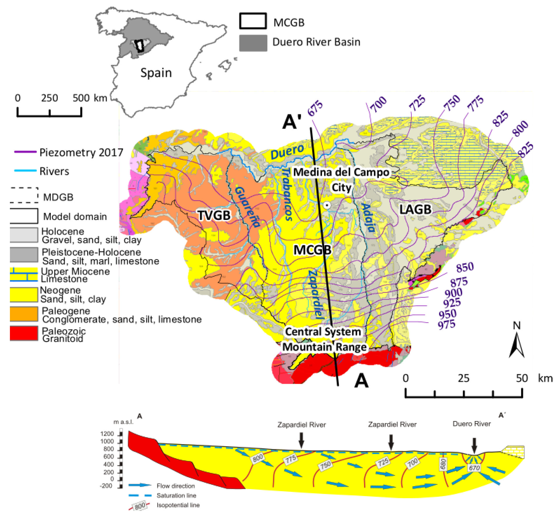
2.1. Location and General Characteristics

The MCGB is situated in the Duero River Basin, in NW Spain (Figure 1), and has a surface area of around 3670 km². The MCGB is bordered by the Duero River to the north, the Central System mountain range to the south, the Adaja River to the east, and the Guareña River to the west [32,33,34]. The average altitude is 812 m a.s.l.; the lowest zone (645 m a.s.l.) is located on the northern edge of the study area, and the highest (1252 m a.s.l.) is located on the southern edge. There is a general decreasing slope from S to N.

The hydrographic network includes the main river courses Adaja, Zapardiel, Trabancos, and Guareña, all flowing to the Duero River in the north (Figure 1). A few decades ago, there were many small groundwater-associated wetlands, but almost all of them are now dry.

Although the NAIAD project focused on the MCGB, for a better understanding and definition of the boundary conditions two more groundwater bodies have been included in the study: Los Arenales (LAGB) and Tierra del Vino TVGB), placed to the E and to the W of the Medina del Campo, respectively (Figure 1). Some results will refer to the three groundwater bodies, but most will refer just to the MCGB.

The area has a Mediterranean climate characterized by hot summers and cold winters, with a mean annual temperature of 12 °C (between the years 1940 and 2005) [35]. Winter values are around 4 °C, and summer values are around 22 °C. Average annual precipitation over the basin is 404 mm, most of it taking place in autumn. Average annual potential evapotranspiration is 750 mm [34,35,36,37,38]. The area is prone to climatic and geomorphological hazards such as floods, droughts, and soil erosion.

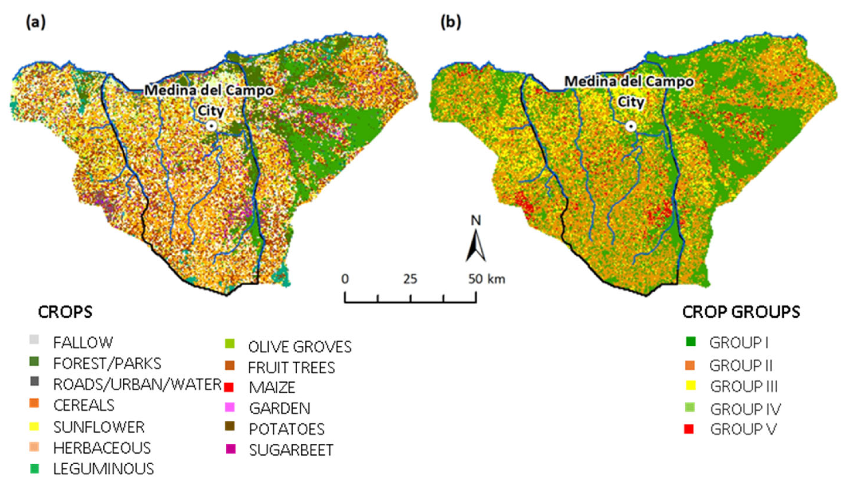
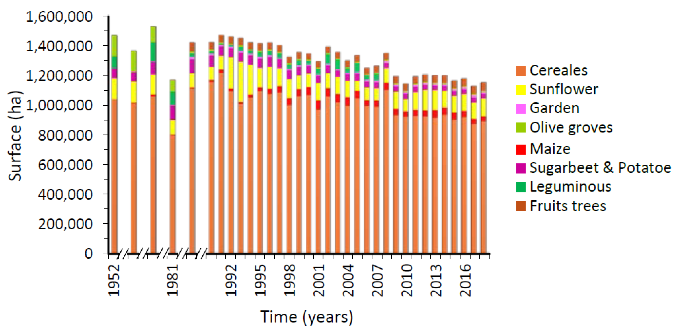
2.2. Water and Land Use

The MCGB spreads across five different provinces, with 130 municipalities and 70,000 inhabitants. The economy is mainly agricultural, with about 3200 km² of cultivated area and only 39 km² of urban surface. Medina del Campo city is the only town with a significant industrial and services sector. The rest of the surface is covered by forests and scrub vegetation, mainly with species from the pine family (Pinus pinea, Pinus pinaster) or poplars (Populus nigra, Populus alba) [34]. Currently, riparian forests are located only in the Duero and Adaja rivers (in the latter, artificially reintroduced). In the other rivers, riparian forests have disappeared, mainly due to water-table drawdown because of aquifer overexploitation [39]. Rain-fed crops, primarily consisting of cereals, legumes, and sunflowers, dominate in the MCGB; irrigated crops, including beet, potato, corn, and rapeseed, represent only 10% of the total cultivated area [40].

The Autonomous Region of Castilla y León, where the MCGB is located, is Spain’s largest fertilizer consumer, with a total of 441,378 tons used in 2020. This represents 22.69% of the total national consumption, and has increased 19.58% since 2010 [41].

The MCGB provides diverse ecosystem services to humans and the environment, such as water supply for small villages and agricultural irrigation [42], and support for aquatic surface ecosystems (wetlands, riverine forests, and streams). However, agricultural intensification, overuse of fertilizers since the late 1970s, and intensive groundwater exploitation from the mid-1970s to the early 2000s have severely reduced and degraded groundwater quality and quantity.

2.3. Geology and Hydrogeology

The MCGB is part of the large Duero River sedimentary basin. With a tectonic origin, the basin is filled with eroded materials from several mountain ranges that isolated the basin for hundreds of years. The geological basement consists of Paleozoic igneous and metamorphic rocks [43]. The filling is composed of Tertiary sediments, mainly fine alluvium, eolian deposits, and a silty-sandy-marly matrix of lacustrine origin with gypsum layers in the northeast, deposited during the Paleogene and Neogene [44], though most sediments date to the Upper-Middle Miocene. Plio–Quaternary deposits include alluvial terraces and extensive eolian sandy layers [45]. The total sediment thickness increases from 500 m in the south to 2000 m in the north, influenced by deep regional faults that affect the basement and part of the sedimentary filling [34,35,36,37,38,39,40,41,42,43,44,45,46,47].

Despite high textural heterogeneity, the sedimentary fill behaves as a well-connected multilayer aquifer system. The upper part forms a heterogeneous (sometimes discontinuous) water-table aquifer, while deeper layers act as a semi-confined to confined system, with silty layers acting as aquitards. According to this, the conceptual hydrogeological model is a system formed by three more or less continuous layers: (1) a semiconfined lower aquifer, composed of Paleogene sands, silts, and gravels reaching depths of up to 2000 m near the Duero River to the north; (2) an intermediate aquitard, consisting of Neogene fine-grained sediments with a thickness ranging from 35 to 50 m; and (3) an upper aquifer, formed by Plio–Quaternary gravel, sand, and conglomerates with up to 15 m thickness [38,39,40,41,42,43,44,45,46,47,48]. The hydraulic permeability is high in the Quaternary alluvial and eolian sands (>10² m/day), and low in the Tertiary sediments (between 10⁴ and 10² m/day) [48].

Natural recharge occurs through rainfall infiltration, with slow groundwater transfer through the aquitard from the upper to the lower aquifer. The regional horizontal groundwater flow is from the south to the north, according to [34] (Figure 1). From the groundwater resources accounting standpoint, irrigation does not contribute additional recharge, as it relies on local groundwater. However, from the management and environmental angle, groundwater pollution due to excess irrigation water recharge is a very relevant issue [48].

Until the mid-20th century, natural groundwater discharge in the MCGB upper aquifer occurred through evapotranspiration and to the surface drainage network. Since the mid-1970s, natural discharge has been progressively substituted by groundwater abstraction for irrigation and for the supply of small towns. Pumping intensification during the 1980s and 1990s led to lowered groundwater levels by up to 30 m between 1972 and 2012 [49], and disconnected rivers and wetlands from the saturated zone. Today, only the Duero and the Adaja rivers maintain a permanent flow (the last one due to river regulation by dams), while the other rivers in the zone only have flow after heavy rainfall. Natural discharge from the deeper, semiconfined layer occurs toward the Duero River and through groundwater abstraction.

Groundwater chemical composition in the MCGB is mainly of the calcium–magnesium bicarbonate, calcium–sodium bicarbonate, and sulfate–calcium facies. The electrical conductivity ranges from 150 to 1500 μS/cm, with average values around 500 μS/cm. Nitrate concentrations vary between 0 and 100 mg/L in the whole aquifer system (DRBA database for the period 1977–2019) [42].

3. Methodology

The study methodology consisted of selecting a specific GWES adequately representing groundwater quality problems in the MCGB. The actual situation and possible future evolution of this GWES were assessed under different groundwater and fertilizer management scenarios with a nitrate transport numerical model. In this section, we describe the numerical model first and provide details on the methodology used to assess the selected GWES later.

3.1. Identification of the Groundwater Ecosystem Service to Be Evaluated

According to DRBA [32,33,34,35,36,37,38,39,40,41,42,43,44,45,46,47,48,49,50,51], one of the most severe problems in the MCGB is the risk of not complying with the environmental quantity and quality objectives of the European Union for the year 2027. Increased agricultural production, intensive use of fertilizers, and excessive groundwater exploitation for agricultural irrigation have caused severe problems. Groundwater contamination in the MCGB by nitrate reached concentrations of 190 mg/L. Thus, the provision of groundwater with good quality for human consumption is not suitable in many parts of the area.

Due to the relevance of this problem, we selected a specific GWES related to water quality to evaluate its current status and the probable future evolution under different scenarios, the Abiotic Provisioning Service Groundwater of Good Quality for Human Supply (APS-GWGQHS), as classified under the European Union’s Common International Classification of Ecosystem Services (CICES) [52]. In the MCGB, this service reflects the aquifer system’s ability to provide water suitable for human use. Improving the provision of this service requires reducing nitrate concentrations in groundwater.

3.2. Nitrate Transport Numerical Model

A nitrate transport numerical model was developed to assess the current state and future evolution of the selected GWES. The numerical model is based on an existing groundwater flow numerical model covering the period from 1950 to 2018, which was calibrated to present-day conditions. This flow model is based on the three-dimensional MODFLOW 2005 [53] code, which solves groundwater flow equations in porous media, using the finite difference method. MODFLOW [53,54] can simulate both steady and transient state flow across multiple layers and different types of aquifers. Specific details about this numerical model can be found in [9]; only the main aspects are presented here.

The modelled area covers a surface of 8728.75 km², with the MCGB occupying 3702.75 km² in the central part of the zone (Figure 1). The whole model domain is discretized into 34,915 active quadrilateral cells, each measuring 500 × 500 m. It has three layers: (1) the upper layer represents the unconfined aquifer, extending down to a depth of 15 m; (2) the intermediate layer represents the aquitard, from 15 to 50 m, which does not contribute to the evaluated ecosystem service; and (3) the lower layer represents the semiconfined aquifer, which ranges from 50 m to the geological basement. The simulation period extends from 1950 to 2018, with 1950 representing nearly undisturbed conditions. The simulation time step is one year.

Key parameters such as hydraulic conductivity (K), storage coefficient (S), and pumping rates were manually calibrated using piezometric data from 1950 to 2018, and historical records of groundwater extractions obtained from the databases and other documents of the DRBA and the Geological and Mining Institute of Spain (see data sources and additional details in [9]). The lower layer was divided into 17 hydraulic conductivity zones based on hydrogeological maps covering the study area [48]. The flow model was calibrated using this zoning and the piezometric time series of 102 observation points scattered across the full modeled domain. Despite the relatively coarse grid resolution and annual time steps, the model achieved an average absolute error of 12 m for the full modelled area and 11 m for the MCGB subarea, with a regression coefficient of 0.962 (Figure S1). This high level of accuracy makes the model reliable for groundwater forecasting at a regional scale.

For the forecasting simulations of the flow model, two types of scenarios were considered: groundwater exploitation management and climate change projections. The groundwater exploitation scenarios were:

(1)

Maintaining current abstraction rates (Business as Usual, BAU).

(2)

Reducing abstractions to an Exploitation Index (EI) = 0.8 by the year 2050, in alignment with the settled objectives of the Duero River Basin Authority. The EI is the mean annual total withdrawal of groundwater relative to the average annual groundwater renewable resources.

Climate change scenarios were based on Representative Concentration Pathways (RCPs) commonly used in regional hydrological assessments:

(A)

RCP 4.5, corresponding to a moderate stabilization scenario. It was associated with a projected 3% increase in annual precipitation in the study area, based on climate change analyses of a climate-change specialist NAIAD partner.

(B)

RCP 8.5, a high-emission scenario. It was associated with an 8% decrease in precipitation in the area, based on national assessments (CEDEX, 2017).

(C)

A No-Change scenario was also included as a baseline.

Climate change simulations were implemented as changes in groundwater recharge. To simulate future recharge, the model assumed that the current recharge coefficient (ratio of recharge to precipitation) remained constant throughout the simulation period. This ratio was applied to the projected precipitation time series for each climate scenario to generate extended recharge inputs.

The results of the prospective flow model indicated that precipitation changes had a relatively minor effect on groundwater levels when compared to the impact of controlling groundwater abstraction [9]. Following this result, in the nitrate transport model we retained only the two groundwater management scenarios (BAU and EI = 0.8) and assumed stable climatic conditions, focusing on the most influential and policy-relevant drivers of aquifer response.

The code MT3DMS [55] was coupled with MODFLOW 2005 [53] to simulate nitrate transport. This code simulates how groundwater contaminants, like nitrate (NO₃⁻), change over time due to advection, dispersion, and chemical reactions, and considers different sources and sinks for contaminants.

Nitrate concentrations in groundwater were simulated in a three-step approach: (1) in order to quantify nitrogen (N) input to the unsaturated zone, two models based on empirical data were developed to obtain information on the spatial and temporal evolution of N supply to the soil in the study area between years 1950 and 2018; (2) to generate a N input time function to groundwater for the numerical model, several models were used to estimate N input to the aquifer saturated zone between years 1950 and 2018. The results were converted to equivalent nitrate (NO₃⁻) concentrations and compared to measured NO₃⁻ values in the MCGB, and the model best matching the observations was used to assess the present state and the future evolution of the evaluated groundwater ecosystem service; and (3) the NO₃⁻ input model selected in step 2 was used to assess the possible future evolution of the ecosystem service.

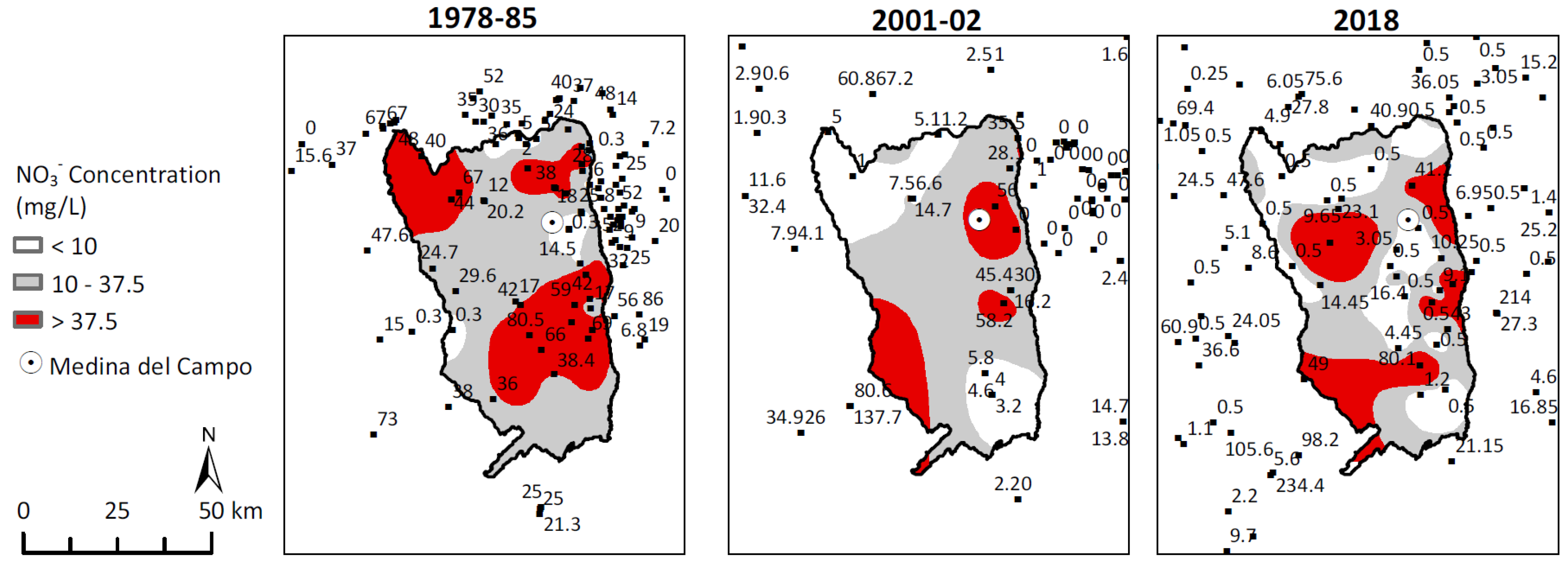
3.2.1. Nitrate Observations

Nitrate historical data in groundwater were obtained from the DRBA database of the groundwater quality observation network. Chemical analyses with ionic balance errors greater than 10% were discarded. As a result, 352 data records from 172 observation points were used for the study of NO₃⁻ spatial and temporal evolution.

A major portion of the data was obtained from observation boreholes deeper than 50 m, which tap the lower aquifer layer. For many of them, there is neither geological nor technical information, and they probably mix water from all layers. Due to the lack of information, data were grouped and analyzed in two depth ranges: ≤50 m, representing the Upper Aquifer and Aquitard layers together, and >50 m, representing the Lower Aquifer layer. However, due to the mentioned potential mixing of water from different flow lines at observation points with long screens, there is notable uncertainty about which depth represents the data.

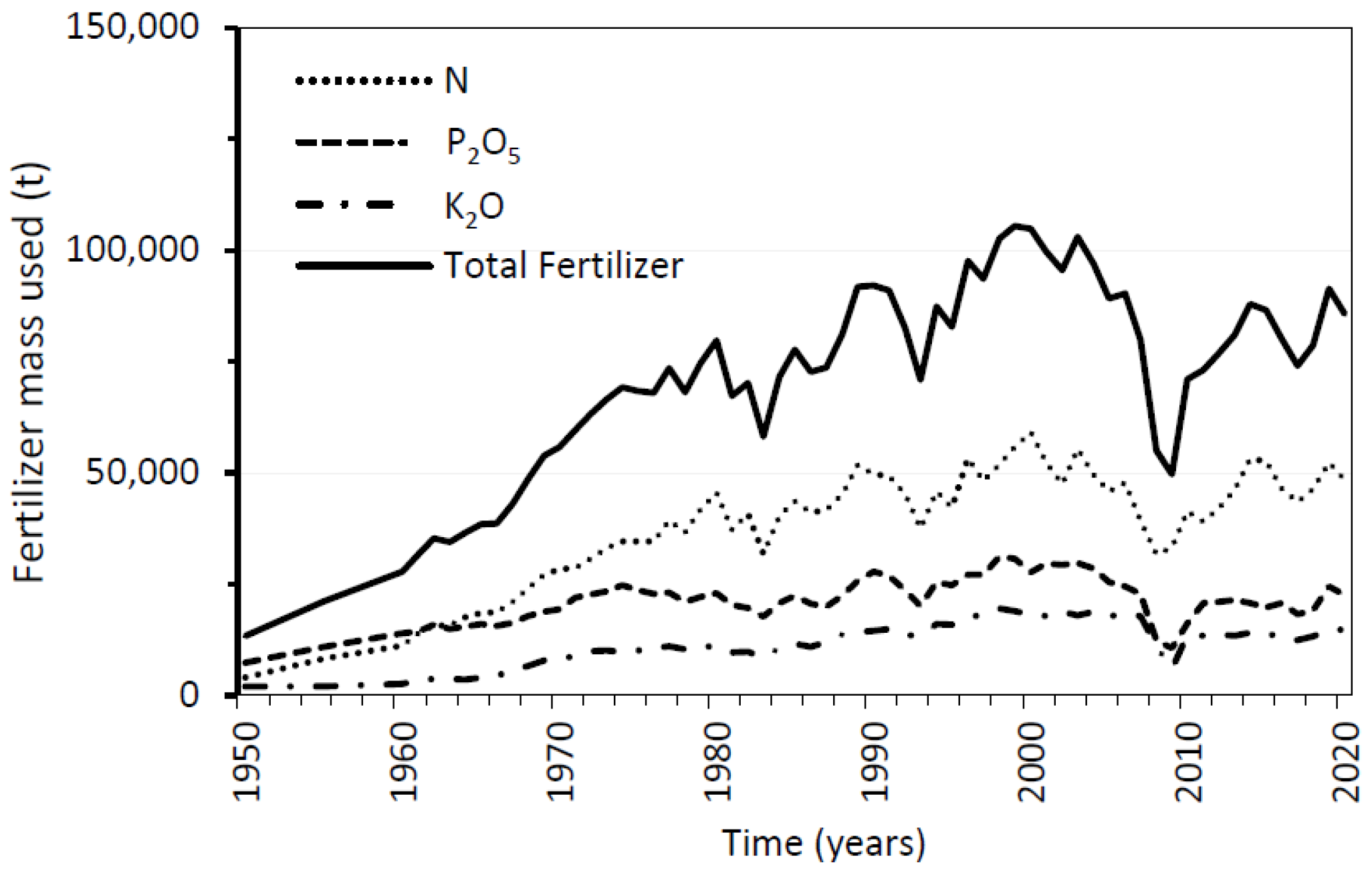
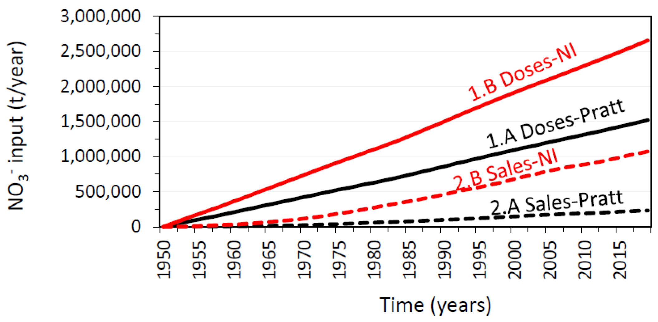
3.2.2. Temporal and Spatial Evolution of Nitrogen Supply to the Soil

The following data were integrated to estimate nitrogen (N) supply to the soil in the study area: the official 2018 land-use map [40]; N doses recommended for the crops in the area [56]; temporal evolution of surfaces cultivated with different crops [57,58,59]; and fertilizers sales history, both in Spain [60] and in the Autonomous Community of Castilla and León [61].

The official crops map of the year 2018 includes 42 crop classes, natural surfaces, and urban areas, grouped into various categories with a total surface of 8728.75 km². To ease the next steps, this map was simplified by grouping the original categories into five broader types: Group 1 includes fallow land, forest and park areas, and urban zones such as roads and water bodies; Group 2 corresponds to cereals; Group 3 comprises sunflower, herbaceous, and leguminous crops; Group 4 includes olive groves and fruit trees; and Group 5 consists of maize, garden crops, potatoes, and sugar beet. This reclassification reduced the complexity of the original map while preserving essential agricultural characteristics for the modeling process. The original map and the one resulting from this simplification are shown in Figure 2.

After map simplification, the surface area requiring N fertilization (mainly dominated by cereals) was 5620.5 km², and the surface area not requiring N fertilization (forest vegetation, fallows, natural, urban, and other surfaces) was 3108.25 km².

Given the uncertainties associated with the type of data and the spatial and temporal scales, two methods were used to better account for the N input to the soil: Method 1 is based on cultivated surface data and recommended N doses for the five crop groups in Figure 2, while Method 2 is based on available N fertilizer sales data and their temporal evolution.

Method 1. Nitrogen input to the soil based on the modified land-use map, recommended doses, and the temporal evolution of the cultivated surface.

To estimate N supply to the soil using the simplified crops map, an average value of N doses for each crop group was calculated using the recommended N doses for each individual crop within the group, weighted by its area.

The temporal evolution of the cultivated area in the study zone between the years 1952 and 2018 was analyzed to build an N input time function for the numerical model. Raw data were obtained from the Spanish National Statistics Institute, the Autonomous Community of Castilla and León, and the Spanish Ministry of Agriculture, Fisheries and Food [57,58,59], and was elaborated as shown in Figure 3. The figure shows that the cultivated surface has been decreasing since the early 1990s. According to Seoane [62], this could be due to several different causes: crop abandonment as a result of new agricultural terms and regulations promoted by the European Union since the late 1980s; emigration from rural to urban areas; population aging [63]; and decreased precipitation (for rain-fed crops) [64], among others.

Method 2. Nitrogen input to the soil according to fertilizer sales.

The recorded N fertilizer consumption was analyzed at the regional [59] and national [60] scales. Data were collected for the entire country for the period 1950–2005, and for the Autonomous Community of Castilla and León from 2005 onwards. The available data were extrapolated to the total modelled surface. Figure 4 shows the evolution of fertilizer sales extrapolated to the modelled area from 1950 to 2018.

3.2.3. Nitrogen Leaching to Groundwater

To generate representative data of NO₃⁻ input to groundwater, two methods were used to account for nitrogen leaching from the soil to the saturated zone of the aquifer: Method A used the Pratt equation [65], and Method B used the Nitrogen Index (NI) model [66].

Method A. Nitrogen leaching to the saturated zone according to the Pratt equation.

Fertilizers are essential for profitable agricultural production [67], but intensive farming has led to increased use in recent decades. Fertilizer overdoses are not absorbed by crops, leading to N losses to the atmosphere and runoff, or to N moving below the root zone [68], eventually leaching into the saturated zone and thus polluting groundwater [69].

The reviewed studies show wide ranges of N leaching to the saturated zone with respect to the total N applied: 14% to 38% [68,69,70], 10% to 30% [71], or 25% [5]. Ramos et al. [69] estimated losses for crops like onion, potatoes, and citrus using the empirical equation of Pratt (Equation (1)), which considers that 20% of N applied leaches to the soil [65]:

$$N_L=0.20\times (N_i\times {D)}^{0.712}$$

(1)

where:

$N_L$ is N leaching to the saturated zone (kg/ha/year),

$N_i$ is the maximum recommended N dose (kg/ha/year),

$D$ is recharge to the water table in cm/year.

Method B. Nitrogen leaching to the saturated zone according to Nitrogen Index.

This method used the Nitrogen Index (NI) software (Version 1.0) [66] to calculate leaching percentages by estimating the annual balance of N inputs and outputs in the soil and its availability for subsequent crops. The model included different crop combinations and different N doses, both under rain-fed and irrigated conditions.

A total of 14 simulations were conducted, applying the maximum recommended N doses (kg/ha/yr). The range of leaching percentage calculated by NI goes from 5 to 35.6%, with an average value of 10.25%.

Table 1. Nitrogen leaching for the considered crop groups, calculated with Nitrogen Index.

Crop Groups	N applied to Soil (kg/ha/yr)	N leaching to the Saturated Zone (%)	N Leaching to the Saturated Zone (kg/ha/yr)
Group I	0	0	0
Group II	40	5	2
Group III	50	5	2.5
Group IV	110	16.6	18.26
Group V	250	35.6	89

shows the percentage of N leaching for the considered crop groups.

These methods were combined with the two methods used to estimate N input to the soil, resulting in four models to reproduce N input to the saturated zone (

Table 2. Models initially used to estimate nitrogen input to groundwater.

		Nitrogen (N) Application
		Method 1. Recommended N Doses and Temporal Evolution of Cultivated Surface Per Crop Groups	Method 2. Temporal Evolution of N Fertilizer Sales
Nitrogen leaching to groundwater	Method A. Pratt equation	1.A. Doses + Pratt	2.A. Sales + Pratt
	Method B. Nitrogen Index model	1.B. Doses + NI	2.B. Sales + NI

). A numerical model was implemented and run for each of the four models, and the one whose results were most coherent with the observed values of NO₃⁻ was selected and subsequently calibrated to evaluate the future management scenarios considered by the DRBA. Model 1.B Doses + NI was selected as the best representation of the conditions in the studied zone (see Section 4.1).

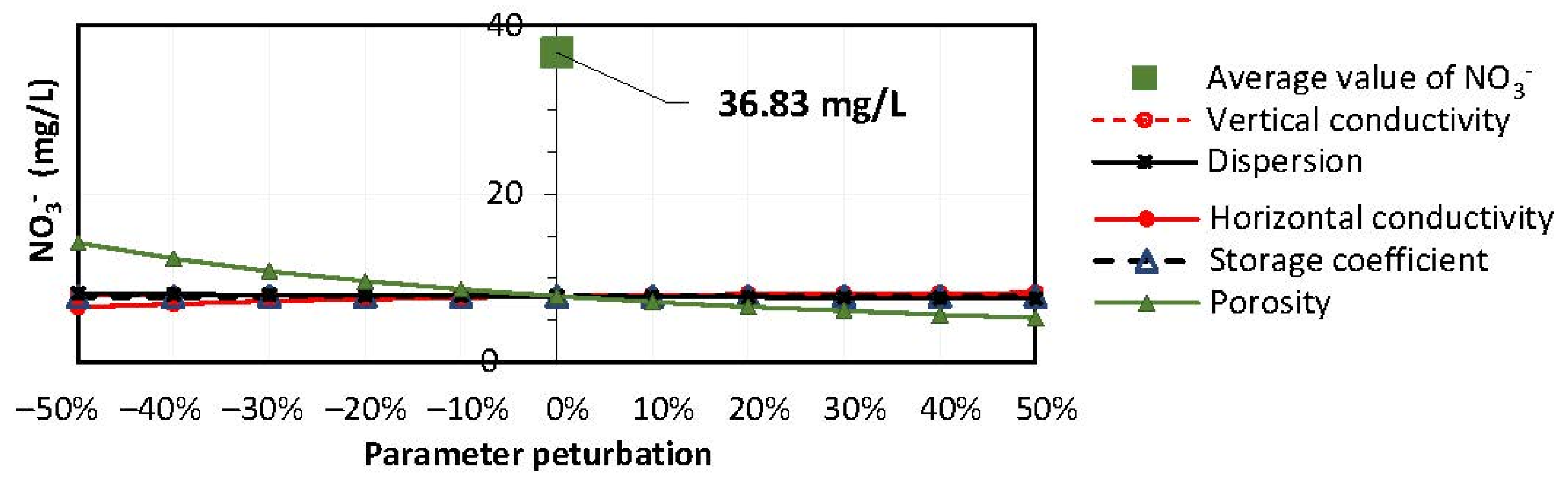
3.2.4. Sensitivity Analysis of Transport Parameters

Given the uncertainties associated with the nitrate observations and the regional scope of the model, full calibration was not feasible. To enhance the utility of the model, a sensitivity analysis was conducted on key parameters that influence NO₃⁻ concentrations, such as the hydraulic conductivity, porosity, storage, and the dispersion coefficient. A relative sensitivity criterion was applied as defined by Equation (2):

$${\displaystyle \frac{CR}{CP}}={\displaystyle \frac{(R_a-R_b)/R_b}{\left(P_a-P_b\right)/P_b}}$$

(2)

where:

CR is the relative change of NO₃⁻ concentration.

CP is the relative change in each parameter or variable with respect to a reference value (typically, the calibrated values in the flow model). The magnitude of the perturbation was set between −50% and +50% [72,73] relative to the reference model.

P_a y P_b are the values used in the sensitivity analysis of the parameter in question (perturbed value and reference value),

R_a y R_b are the perturbed and reference NO₃⁻ concentration values.

The parameters of the reference model (the one considering Model 1.B Doses + NI for nitrate input to groundwater) to be perturbed were: horizontal hydraulic conductivity Kh = 0.008 to 20 m/day; vertical hydraulic conductivity Kv = 0.0001 to 0.1 m/day; and specific storage S = 0.0001 to 0.1. A dispersion value of 1000 m was assigned.

The sensibility analysis performed indicated that porosity is the most influential parameter on NO₃⁻ concentrations in a similar magnitude (Figure 5). Based on the results of this analysis, the efforts have focused on finding the most representative values for porosity to best reflect the observed conditions.

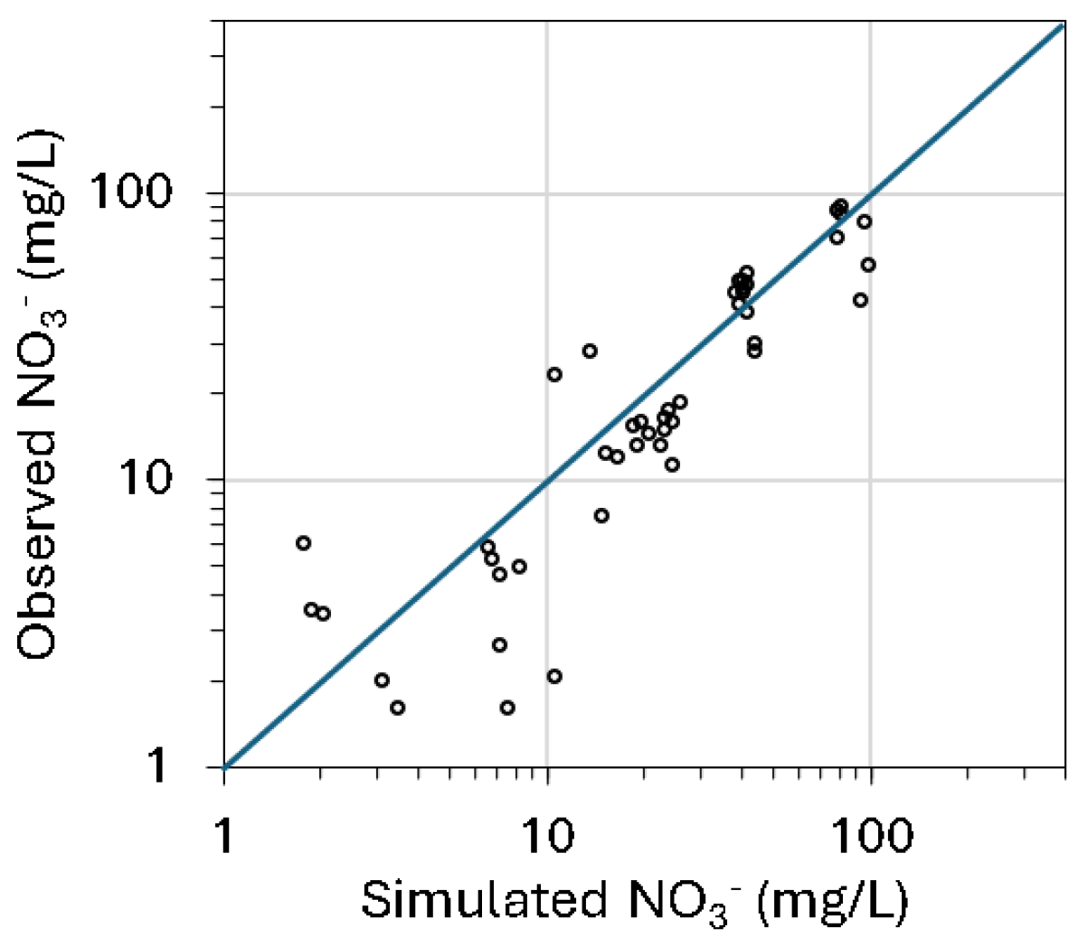
3.2.5. Porosity Calibration

The porosity of the reference model was calibrated for the zones established in the groundwater flow model (see Figure S1). Initial porosity values were derived from the literature for sediments similar to those in the aquifer system [74,75,76]. For layer 1, porosity values were derived from the storage coefficient values used in the flow model, ranging from 0.1 to 0.001, so they were not calibrated.

The initial porosity of layers 2 and 3 was set at 0.25. Those values were manually calibrated and validated (Table S1 and Figure S2) considering the range of porosity values for similar sediment textures reported in the literature [74,75,76], weighted by their thicknesses obtained from lithological columns in the DRBA database [77,78].

Manual calibration of porosity allowed obtaining average NO₃⁻ concentrations in groundwater closer to the observed values at the regional level. Due to the characteristics of the available data (see Section 3.2.1) and the scope of the model, extreme values and local variations of NO₃⁻ concentrations could not be adjusted. The Supplementary Material (Figures S3 and S4) includes temporal evolution graphs of observed and calculated nitrate concentrations for the 75 observation points used.

During porosity calibration, particular emphasis was placed on the public water supply wells, as data from these points are generally more reliable: their technical characteristics—such as screen depth and length—are well known, and the chemical analyses are considered more representative, since these wells are in continuous use and water is renewed. The overall root mean square error (RMSE) between the observed and simulated nitrate concentrations across all observation points was 36.2 mg/L, whereas the RMSE for the subset of supply wells was significantly lower, at 12.2 mg/L. This improved performance is illustrated in Figure 6, which shows observed versus simulated nitrate concentrations for these supply points.

Maximum and average NO₃⁻ values, and number of observation points with concentrations above 37.5 mg/L before and after porosity calibration were compared (

Table 3. Comparison of observed and simulated (with the selected model 1.B) NO₃⁻ concentrations (mg/L) for the period 2000–2018 at two depth ranges, ≤50 m (Upper Aquifer plus Aquitard layers, UAq-Aqt) and >50 m (Lower Aquifer, LAq), before and after porosity calibration.

Observed and Simulated NO3− (mg/L) in Observation Points		Observed	Model 1.B Doses + NI	Model 1.B Doses + NI After Porosity Calibration
Average	UAq-Aqt	54.0	15.5	41.0
	LAq	27.0	0.8	19.6
Maximum	UAq-Aqt	321.5	92.0	166.4
	LAq	220.0	8.0	101.0
Nº of points with NO3− > 37.5 mg/L	UAq-Aqt	78	21	81
	LAq	72	0	23

). Modelled values obtained after porosity calibration approached the observations significantly. Then, given the regional scope of the nitrate model, the calibrated model was used to perform nitrate simulations. The final porosity values (ranging from 0.001 to 0.25) and their spatial distribution are available in Table S1 and Figure S2.

3.3. Assessment of the Current Status of the Groundwater Ecosystem Service Evaluated

The current status of the Abiotic Provisioning Service Groundwater of Good Quality for Human Supply was evaluated by modelling NO₃⁻ concentrations in groundwater by the year 2018. The initial (year 1950) NO₃⁻ values were set to zero, representing natural conditions. As stated, NO₃⁻ inputs to groundwater from fertilizers were modelled using the results of Model 1.B Doses + NI (the N results were converted to equivalent NO₃⁻ concentrations). Nitrate input was introduced as an annual recharge through a mass flow (kg/ha/year). It was assumed that rivers and wetlands do not contribute to NO₃⁻ concentrations and instead act as output zones for NO₃⁻.

The spatial and temporal evolutions of NO₃⁻ concentrations measured in the DRBA observation network were compared to the NO₃⁻ concentrations calculated by the calibrated numerical model. The assessment has been performed using the proportion of aquifer surface area with NO₃⁻ concentrations between 10 and 37.5 mg/L as an indicator. The different number and spatial distribution of NO₃⁻ measured and modelled data make it impossible to extract rigorous information on temporal and spatial changes. Consequently, the transport model was developed using average NO₃⁻ concentration values and could not be optimally calibrated for individual observation points. Nevertheless, the model remains a valuable tool for large-scale basin assessments, considering its limitations. Thus, the model providing the best consistency between modelled and measured NO₃⁻ values in the MCGB was used to assess the present state and the future evolution of the selected ecosystem service.

3.4. Assessment of the Possible Future Evolution of the Groundwater Ecosystem Service Evaluated

The potential future evolution of the selected GWES service was evaluated for two groundwater management scenarios and two fertilizer use scenarios, covering the period from 2018 to 2100. The groundwater management scenarios were based on the Exploitation Index (EI). The two scenarios considered are:

(1)

Business as Usual (BAU): No changes in the EI with respect to the current value in the MCGB (EI = 2.0, according to [9]).

(2)

EI0.8: Reduction in EI from 2.0 to 0.8 by the year 2050 and beyond (this is the target of the DRBA).

The two scenarios related to N fertilizer use are:

(A)

N20%: A linear reduction of 20% in the application of N fertilizers from current numbers (in 2018) by 2030 and beyond.

(B)

ZeroN: A linear reduction in N fertilizer application from current levels (year 2018) to zero by year 2030 and beyond.

Scenario A is the objective set by the Duero River Basin Hydrological Plan for the period 2022–2027, adapted from the European Strategy of the European Green Deal project established at the end of 2019 [51] to reduce nitrate concentrations below 37.5 mg/L by the year 2030 [79]. Although scenario B is improbable, in this work it was considered a theoretical extreme to explore the long-term legacy effects of nitrate contamination.

The evaluation involved simulating NO₃⁻ concentrations in both aquifers and identifying concentration trends along the study period for the four models resulting from combining all the scenarios: 1.A, 1.B, 2.A, and 2.B (

Table 4. Models considered for evaluating the hypothetical future evolution of nitrate concentrations in groundwater.

N Fertilizer Use Scenarios	Groundwater Exploitation Scenarios
	1. IE = BAU	2. IE Reduction to 0.8 by Year 2050 and Beyond
A. 20% reduction by 2030 and beyond	1.A BAU-N20%	2.A EI0.8-N20%
B. Reduction to zero by 2030 and beyond	1.B BAU-ZeroN	2.B EI0.8-ZeroN

).

The relative impact of the different scenarios on the selected GWES was assessed by comparing the aquifer surface areas with different NO₃⁻ concentrations resulting from the four models in Table 4 relative to 2018. Three concentration ranges were considered to perform the comparison: NO₃⁻ < 10 mg/L (unpolluted); NO₃⁻ between 10 and 37.5 mg/L (polluted but under the legal limit); and NO₃⁻ > 37.5 mg/L (polluted beyond the legal limit). The analysis focused on the short-term (by 2050, when both the application of fertilizers and the EI reduction would stabilize) and long-term (by 2100). In addition, the modeled period was extended to evaluate the timeframe over which nitrate concentrations are expected to decrease significantly because of the proposed management measures. Due to the uncertainties associated with projections beyond 2100, all input parameters related to boundary conditions were held constant during this extended simulation period.

4. Results and Discussion

4.1. Nitrate Input to Groundwater

Nitrogen leaching estimations were calculated considering nitrogen (N) masses and concentrations. In order to compare with nitrate (NO₃⁻) observations in the aquifer, the calculated N values were converted to equivalent NO₃⁻ values. Figure 7 shows a summary of the temporal evolution of NO₃⁻ inputs to groundwater in the whole modelled aquifer surface, as simulated by the four leaching models considered.

A clear discrepancy is observed when comparing the nitrogen inputs estimated using recommended agronomic doses with those estimated from fertilizer sales statistics, with sales-based estimates yielding consistently higher values. This difference is primarily attributed to the limitations of the spatial allocation method used to downsize fertilizer sales data to the study area. For data before 2005, national-level fertilizer sales were downscaled to the modelled area using proxies such as agricultural production. After 2005, data from the regional statistics office of the Autonomous Community of Castilla and León were employed. In both cases, data downscaling to the Medina del Campo Groundwater Body involved interpolation based on the extent of cultivated land. This coarse approximation, combined with the lack of detailed farm-level data, tends to underestimate the actual nitrogen applied to crops. These limitations support the selection of the “recommended dose” approach as more consistent with the agronomic reality of the area.

NO₃⁻ concentrations simulated with the four leaching models were compared to observed data from 2000 to 2018, obtained from the groundwater quality observation network of the DRBA. Maximum and average NO₃⁻ concentrations, as well as the number of observation points with concentrations exceeding 37.5 mg/L, were compared for the Upper Aquifer–Aquitard layers together, and for the Lower Aquifer (

Table 5. Comparison of observed and simulated NO₃⁻ concentrations (mg/L) with the four leaching models during the 2000–2018 period at two depth ranges, ≤50 m (Upper Aquifer and Aquitard, UAq-Aqt) and >50 m (Lower Aquifer, LAq).

Observed and Simulated NO3− (mg/L)		Observed	Model 1.A Doses + Pratt	Model 1.B Doses + NI	Model 2.A Sales + Pratt	Model 2.B Sales + NI
Average	Uaq-Aqt	54.0	9.7	15.5	1.9	8.7
	Laq	27.0	0.4	0.8	0.07	0.3
Maximum	UAq-Aqt	321.5	29.0	92.0	8.7	41.8
	LAq	220.0	2.5	8.0	0.3	1.4
Nº of points with NO3− > 37.5 mg/L	UAq-Aqt	78	0	21	0	0
	LAq	72	0	0	0	0

). Model 1.B Doses-NI was selected as the one best representing the observed data.

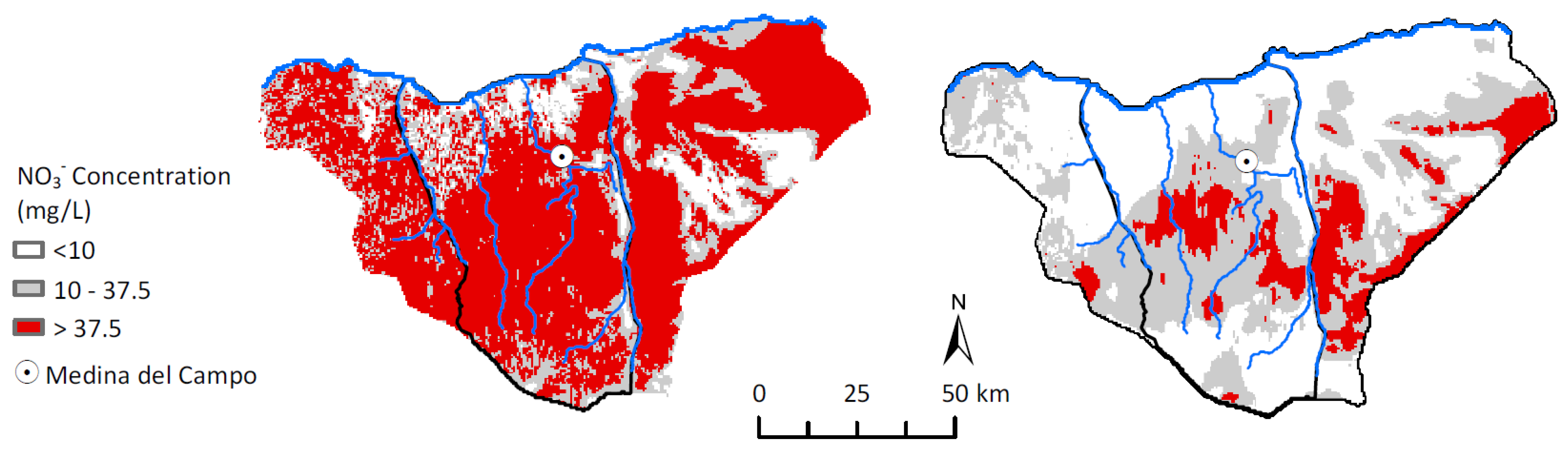
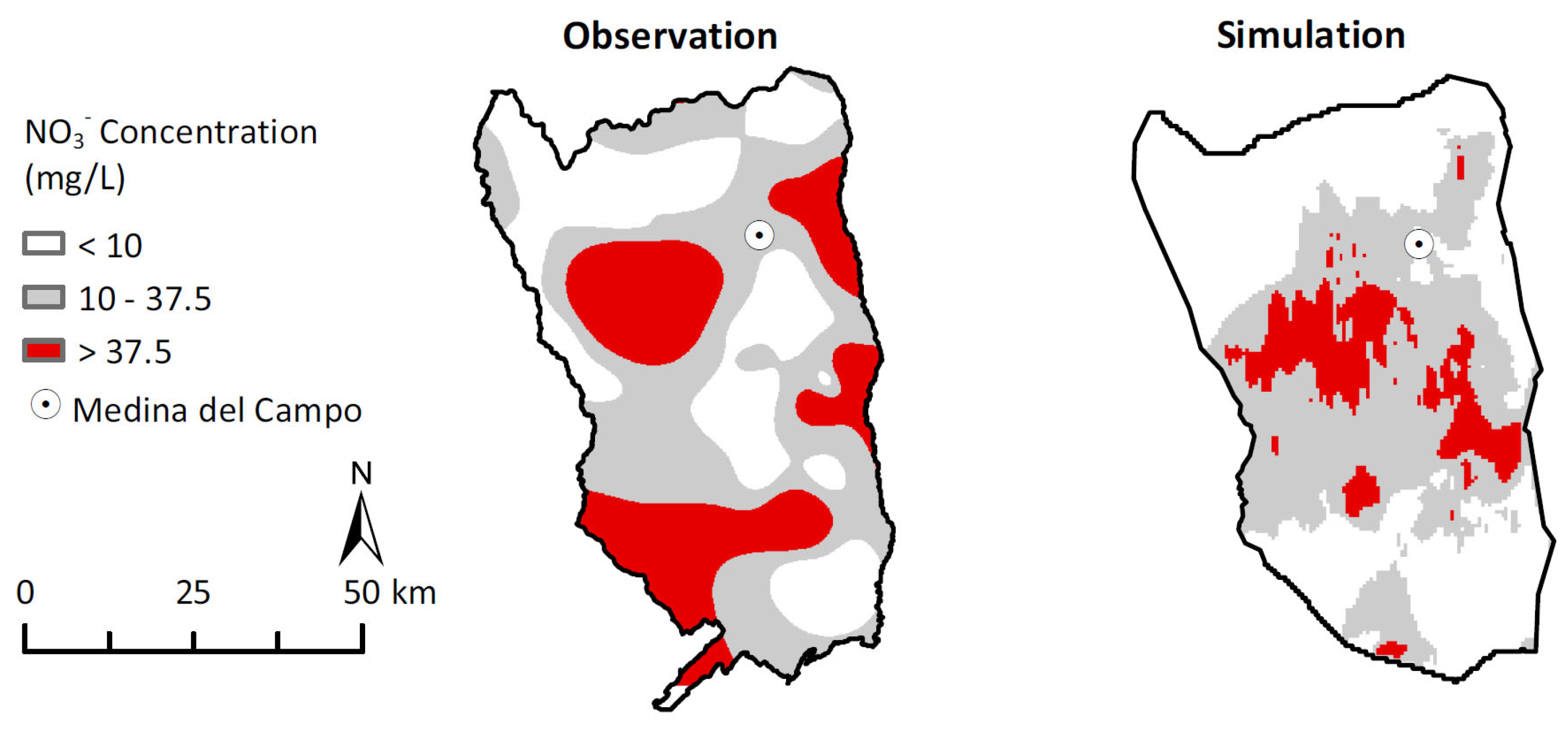
4.2. Assessment of the Current Status of the Abiotic Provisioning Service Groundwater of Good Quality for Human Supply

The assessment of the APS-GGQHS service was based on observing the aquifer surface with nitrate concentrations under 37.5 mg/L. The spatial distribution of NO₃⁻ in groundwater was analyzed by creating maps for three different time periods: 1975–1985 (117 observation points with 224 data records available), 2001–2002 (130 observation points with 213 data records available), and 2018 (325 observation points with 772 data records available). To generate a map for a specific period, enough observed data with accepted analytical quality was required. If the data for a given year were insufficient to support reliable interpolation, a broader period was selected instead. In such cases, concentration averages over the selected period were used to ensure adequate spatial data coverage and to enable the creation of an interpolation map. Many of the observations correspond to the Lower Aquifer, and some correspond to the Aquitard. There were fewer observation points in the Upper Aquifer (4), so it was not possible to create maps for the Upper Aquifer due to data scarcity.

As stated previously, the different number and spatial distribution of observed NO₃⁻ concentration data made it impossible to extract rigorous information on temporal and spatial changes. Moreover, the very different values in nearby boreholes suggest that nitrate values are influenced by local conditions that cannot be adequately represented by a regional model. Thus, a preliminary assessment of the measured data did not reveal clear temporal trends, but significant local changes in NO₃⁻ concentrations (Figure 8).

Despite the impossibility of deducing spatial and temporal nitrate trends at the regional scale from the observations, nitrate values simulated with the porosity-calibrated Model 1.B Doses-NI are realistic on a broad scale (see Table 3). They show that almost 70% of the modelled area in layer one (Upper Aquifer) and 13% in layer three (Lower Aquifer) has NO₃⁻ concentrations higher than 37.5 mg/L (Figure 9). This result suggests that, at present, the status of the Abiotic Provisioning Service Groundwater of Good Quality for Human Supply is of poor quality, and its flow to society is probably nonexistent or close to zero. This is consistent with the fact that in many areas of the MCGB, groundwater cannot be used for human supply.

Figure 10 shows the spatial distribution of observed and simulated NO₃⁻ concentrations in 2018, just in the Lower Aquifer layer of the MCGB. The model cannot reproduce the high NO₃⁻ concentrations observed in the southern part of the MCGB, but it does reasonably reproduce the distribution in the central part. This better model performance for the central area can be explained by the higher data density of the data and the prioritization of calibration water supply wells near Medina del Campo city, while the southern region—characterized by limited data availability and low agricultural pressure—shows greater discrepancies. This model was used to simulate the future evolution of the selected GWES.

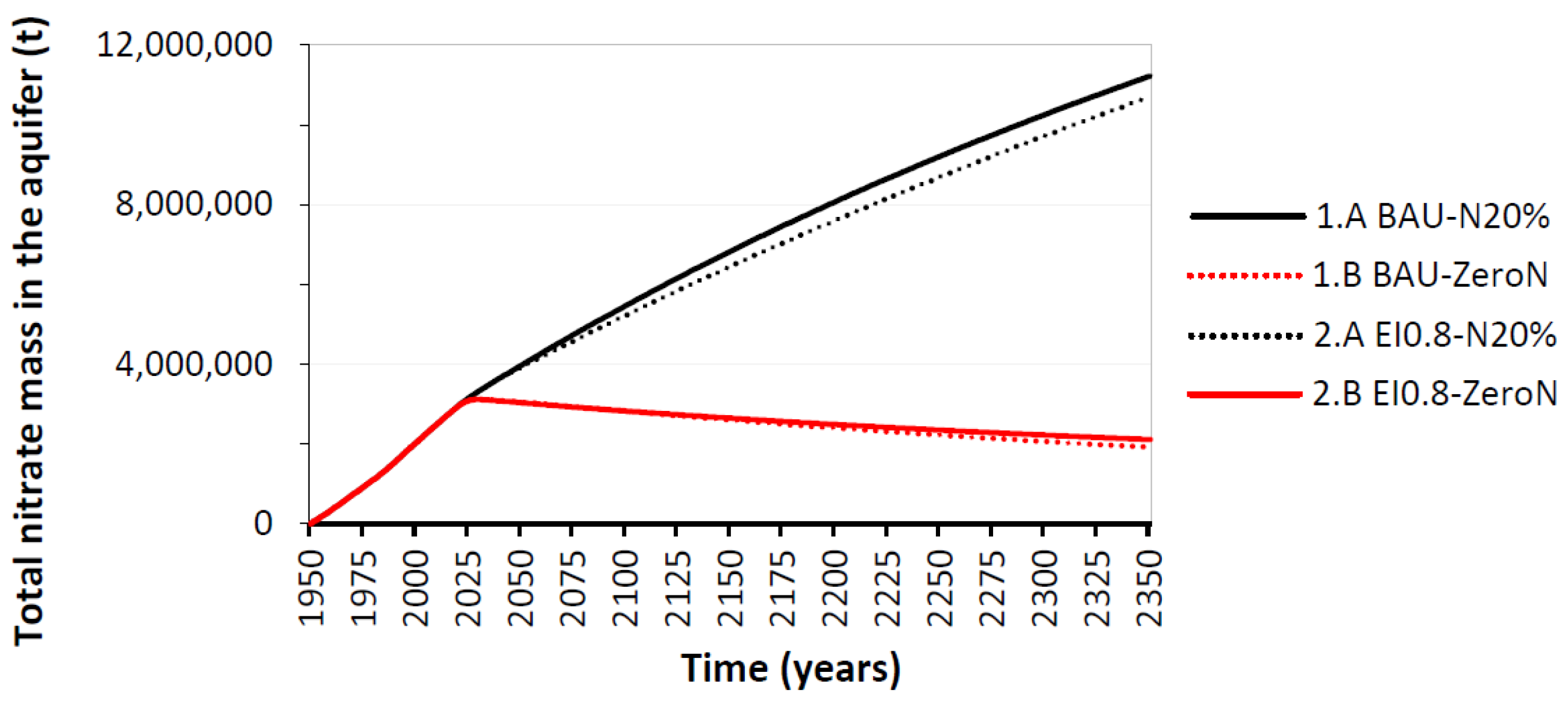
4.3. Assessment of the Possible Future Evolution of the Abiotic Provisioning Service Groundwater of Good Quality for Human Supply

The forecasted temporal evolution of the total mass of NO₃⁻ stored in the aquifer system, simulated with the four models in Table 4, is shown in Figure 11. The spatial distribution of the aquifer surfaces with different NO₃⁻ concentrations resulting from the four models considered is available in the Supplementary Material (Figures S5–S8).

Changes in aquifer surface area with NO₃⁻ > 37.5 mg/L in the years 2050 and 2100 with respect to those in 2018 are summarized in

Table 6. Changes of aquifer surface area with NO₃⁻ > 37.5 mg/L in years 2050 and 2100 relative to year 2018, in layer 1 (Upper Aquifer) and layer 3 (Lower Aquifer), and for the four combinations of future scenarios considered. Changes are expressed as percentages; positive values indicate an increase and negative values indicate a decrease.

N Fertilizer Use Scenarios			Groundwater Exploitation Scenarios
			1. IE = BAU	2. IE Reduction to 0.8 by Year 2050 and Beyond
A. 20% reduction by 2030 and beyond	Layer 1	In 2050	+4.4	+4.8
		In 2100	+7.9	+8.5
	Layer 3	In 2050	+9.4	+8.7
		In 2100	+20.1	+18.2
B. Reduction to zero by 2030 and beyond	Layer 1	In 2050	−49.4	−49.1
		In 2100	−65.9	−65.8
	Layer 3	In 2050	+2.7	+2.5
		In 2100	−4.9	−4.3

, showing percentage increases or decreases for each scenario. The results show that a 20% reduction in fertilizer application by 2030 and beyond leads to continued NO₃⁻ accumulation and a gradual increase in concentrations over time. In models 1.A BAU-N20% and 2.A EI0.8-N20%, the aquifer surface area with NO₃⁻ concentrations above 37.5 mg/L will continue increasing until the year 2100. Only the complete cessation of nitrogen fertilizer use significantly reduces nitrate inputs. According to the extended-time simulation, this scenario would result in a 50% decrease in the surface area affected by nitrate contamination by 2350.

When comparing groundwater management scenarios to nitrogen fertilizer reduction scenarios, the trends in NO₃⁻ concentrations at three observation points in the MCGB (Figure 12) show clearly that reducing fertilizer use has a greater impact on lowering nitrate concentrations than reducing groundwater extractions. These points correspond to public water supply wells, which are of particular relevance for groundwater management, and are spatially well distributed across the groundwater body. Moreover, combining fertilizer cessation and reduced groundwater pumping provides only a marginal additional benefit. Even under the most favorable scenario, the total nitrate mass is expected to be reduced by only about half by 2350, indicating that full recovery to natural conditions would require several centuries.

These results show that neither reducing groundwater abstraction nor reducing fertilizer application—or even stopping it—will significantly improve the conditions in the aquifer for a significant improvement of the Abiotic Provisioning Service Groundwater of Good Quality for Human Supply in the short (by 2030) and medium (by 2050) term. Such significant enhancement of the service would only be possible in the long term (by 2350), and would be achieved mostly by control of fertilizer doses.

4.4. Uncertainty of the Numerical Modelling

The results presented in this study illustrate the utility of numerical modelling to support the assessment of groundwater ecosystem services, with particular focus on the provision of good-quality groundwater for human supply. In particular, the model has proven valuable for estimating the surface area of the aquifer affected by excessive nitrate concentrations under various fertilizer application strategies and groundwater exploitation scenarios. This spatial indicator, aligned with environmental quality objectives, provides a more robust and policy-relevant metric than isolated point concentrations—especially when dealing with regional-scale systems and fragmented monitoring data.

The regional scale of the model (with a horizontal resolution of 500 × 500 m) does not allow for the representation of local heterogeneity or small-scale pollution sources, such as manure hotspots or faulty septic systems. While this resolution is appropriate for simulating broader hydrogeological trends and assessing spatial patterns of contamination, it cannot capture sub-grid variations that may significantly affect nitrate concentrations at individual points.

Several limitations must be acknowledged. First, the observed nitrate concentration data used for calibration and validation suffer from considerable spatial and temporal inconsistencies. The groundwater quality monitoring network lacks systematic coverage and continuity; most wells are fully screened and therefore mix water from multiple depths, which masks vertical gradients and limits interpretability. In many locations, long-term time series are unavailable, and only sporadic measurements exist, particularly in the earlier decades of the simulation period. These limitations hinder the accurate reproduction of point-scale trends in nitrate contamination.

These constraints guided our decision to focus the model evaluation on the consistency of nitrate concentration orders of magnitude and spatial patterns, rather than on matching observed values at specific wells. The model was not intended as a predictive tool for local concentration values, but rather as a means to validate the conceptual model and assess the evolution of the aquifer’s functional status under different management scenarios.

Despite these limitations, the model offers useful insights into the potential for long-term aquifer recovery, the relative importance of land-use versus pumping interventions, and the inertia of nitrate pollution in groundwater systems. The scenarios explored—while not all realistic—serve as boundary conditions that help to delineate the temporal dynamics of ecosystem service provision. In particular, the observed delay between management action and water quality improvement reinforces the importance of early intervention and sustained monitoring.

Finally, the modelling framework developed here supports the ecosystem services assessment by linking physical processes with human benefits in a spatially explicit and policy-relevant way. It enables the identification of vulnerable areas and critical time horizons for action, offering valuable input for planning and decision-making at the aquifer level.

5. Conclusions

This study illustrates how to incorporate the Ecosystem Services Assessment (ESA) approach to evaluate the expected relative impact of different management actions aiming to improve the flow of significant groundwater services to humans, such as the provision of good quality groundwater for human supply. The provisioning service assessed here, the Abiotic Provisioning Service Groundwater of Good Quality for Human Supply, was used as a case study in the Medina del Campo Groundwater Body (Spain), where groundwater quality and use have been severely affected by nitrate pollution due to intensive agricultural practices.

The study results confirm the usefulness of coupling groundwater flow and nitrate transport numerical modelling with the ESA framework to assess both the current status and the potential long-term evolution of the service under various feasible groundwater exploitation and fertilizer use management scenarios. Even though the representativity of the observed data is uncertain and modelling results cannot match them with fidelity, simulated nitrate concentrations reasonably reproduce the order of magnitude and the spatial distribution at a regional scale. This provides confidence in the results and validates the use of groundwater modelling to assess prospective analyses of groundwater ecosystem services.

The analysis of available nitrate concentration data revealed widespread contamination, with concentrations exceeding the regulatory limit of 37.5 mg/L for human consumption in several areas of the studied groundwater body, reaching up to 212 mg/L in some zones. After refining the dataset to include only observation points with acceptable ionic balance, the assessment showed that nitrate contamination has substantially reduced the capacity of the aquifer to provide good quality water, and also that this degradation will continue over time.

Model simulations indicate that a 20% reduction in nitrogen fertilizer use, as proposed in current EU strategies, will be insufficient to reverse nitrate contamination even in the long term (up to the year 2100). Only a complete cessation of fertilizer application would lead to significant improvements, with a projected 50% reduction in nitrate concentrations in the very long term (by 2350), provided no major climate changes occur. These results underscore the urgent need to implement stricter nitrogen management policies and to consider multi-decadal recovery horizons when designing effective groundwater protection strategies.

Overall, the findings highlight that without ambitious and sustained reductions in fertilizer inputs, the availability of the Abiotic Provisioning Service Groundwater of Good Quality for Human Supply will continue to decline well beyond the year 2050.

References

1. Harrison, S.; McAree, C.; Mulville, W.; Sullivan, T. The problem of agricultural ‘diffuse’ pollution: Getting to the point. Sci. Total Environ. 2019, 677, 700–717. [Google Scholar] [CrossRef] [PubMed]
2. Vinod, P.N.; Chandramouli, P.N.; Koch, M. Estimation of Nitrate Leaching in Groundwater in an Agriculturally Used Area in the State Karnataka, India, Using Existing Model and GIS. Aquat. Procedia 2015, 4, 1047–1053. [Google Scholar] [CrossRef]
3. Gleeson, T.; Wada, Y.; Bierkens, M.F.P.; van Beek, L.P.H. Water balance of global aquifers revealed by groundwater footprint. Nature 2012, 488, 197–200. [Google Scholar] [CrossRef] [PubMed]
4. Worrall, F.; Davies, H.; Burt, T.; Howden, N.J.K.; Whelan, M.J.; Bhogal, A.; Lilly, A. The flux of dissolved nitrogen from the UK—Evaluating the role of soils and land use. Sci. Total Environ. 2012, 434, 90–100. [Google Scholar] [CrossRef] [PubMed]
5. Galloway, J.N.; Dentener, F.J.; Capone, D.G.; Boyer, E.W.; Howarth, R.W.; Seitzinger, S.P.; Asner, G.P.; Cleveland, C.C.; Green, P.A.; Holland, E.A.; et al. Nitrogen Cycles: Past, Present, and Future. Biogeochemistry 2004, 70, 153–226. [Google Scholar] [CrossRef]
6. Griebler, C.; Avramov, M. Groundwater ecosystem services: A review. Freshw. Sci. 2015, 24, 355–367. [Google Scholar] [CrossRef]
7. Abbasi, M.R.; Sepaskhah, A.R. Nitrogen leaching and groundwater N contamination risk in saffron/wheat intercropping under different irrigation and soil fertilizers regimes. Sci. Rep. 2023, 13, 6587. [Google Scholar] [CrossRef]
8. Aziz, T.; Frey, S.K.; Lapen, D.R.; Preston, S.; Russell, H.A.J.; Khader, O.; Erler, A.R.; Sudicky, E.A. Economic valuation of subsurface water contributions to watershed ecosystem services using a fully integrated groundwater–surface-water model. Hydrol. Earth Syst. Sci. 2025, 29, 1549–1568. [Google Scholar] [CrossRef]
9. Borowiecka, M.; Alcaraz, M.; Manzano, M. Assessment of Ecosystem Services with numerical modelling to support groundwater dependent ecosystems and aquifer management: A demo study in the Medina del Campo Groundwater Body, Spain. Case Stud. Chem. Environ. Eng. 2024, 10, 100914. [Google Scholar] [CrossRef]
10. Saccò, M.; Mammola, S.; Altermatt, F.; Alther, R.; Bolpagni, R.; Brancelj, A.; Brankovits, D.; Fišer, C.; Gerovasileiou, V.; Griebler, C.; et al. Groundwater is a hidden global keystone ecosystem. Glob. Change Biol. 2024, 30, 17066. [Google Scholar] [CrossRef]
11. Nsoh, W. Achieving Groundwater Governance: Ostrom’s Design Principles and Payments for Ecosystem Services Approaches. Transnatl. Environ. Law. 2022, 11, 381–406. [Google Scholar] [CrossRef]
12. Griebler, C.; Malard, F.; Lefébure, T. Current developments in groundwater ecology—From biodiversity to ecosystem function and services. Curr. Opin. Biotechnol. 2014, 27, 159–167. [Google Scholar] [CrossRef] [PubMed]
13. Bastani, M. Source area management practices as remediation tool to address groundwater nitrate pollution in drinking supply wells. J. Contam. Hydrol. 2019, 226, 103521. [Google Scholar] [CrossRef] [PubMed]
14. Yang, L.; Zheng, C.; Andrews, C.B.; Wang, C. Applying a Regional Transport Modeling Framework to Manage Nitrate Contamination of Groundwater. Groundwater 2021, 59, 292–307. [Google Scholar] [CrossRef]
15. Whiteis, A.M.; Zou, C.B.; Joshi, O.; Ferguson, B.; Roberts, S. Quantitative assessment of ecosystem services in diverse land uses within the forest-grassland transition zone of southern Great Plains, USA. Ecosyst. Serv. 2025, 71, 101697. [Google Scholar] [CrossRef]
16. Lovrić, M.; Torralba, M.; Orsi, F.; Pettenella, D.; Mann, C.; Geneletti, D.; Plieninger, T.; Primmer, E.; Hernandez-Morcillo, M.; Thorsen, B.J.; et al. Mind the income gap: Income from wood production exceed income from providing diverse ecosystem services from Europe’s forests. Ecosyst. Serv. 2025, 71, 101689. [Google Scholar] [CrossRef]
17. Kok, S.; Le Clec’h, S.; Penning, W.E.; Buijse, A.D.; Hein, L. Trade-offs in ecosystem services under various river management strategies of the Rhine Branches. Ecosyst. Serv. 2025, 72, 101692. [Google Scholar] [CrossRef]
18. Sheng, J. Collaborative models and uncertain water quality in payments for watershed services: China’s Jiuzhou River eco-compensation. Ecosyst. Serv. 2024, 70, 101671. [Google Scholar] [CrossRef]
19. Younesi, M.; Saadatpour, M.; Afshar, A. Integration of the system of environmental economic accounting-ecosystem accounting (SEEA-EA) framework with a semi-distributed hydrological and water quality simulation model. Ecosyst. Serv. 2024, 70, 101672. [Google Scholar] [CrossRef]
20. Peña, L.; de Manuel, B.F.; Méndez-Fernández, L.; Viota, M.; Ametzaga-Arregi, I.; Onaindia, M. Co-Creation of Knowledge for Ecosystem Services Approach to Spatial Planning in the Basque Country. Sustainability 2020, 12, 5287. [Google Scholar] [CrossRef]
21. Peña, L.; Onaindia, M.; de Manuel, B.F.; Ametzaga-Arregi, I.; Casado-Arzuaga, I. Analysing the Synergies and Trade-Offs between Ecosystem Services to Reorient Land Use Planning in Metropolitan Bilbao (Northern Spain). Sustainability 2018, 10, 4376. [Google Scholar] [CrossRef]
22. Murray, B.R.; Hose, G.C.; Eamus, D.; Licari, D. Valuation of groundwater-dependent ecosystems: A functional methodology incorporating ecosystem services. Aust. J. Bot. 2006, 54, 221. [Google Scholar] [CrossRef]
23. Danielopol, D.L.; Gibert, J.; Griebler, C.; Gunatilaka, A.; Hahn, H.J.; Messana, G.; Notenboom, J.; Sket, B. Incorporating ecological perspectives in European groundwater management policy. Environ. Conserv. 2004, 31, 185–189. [Google Scholar] [CrossRef]
24. Quevauviller, P. Groundwater monitoring in the context of EU legislation: Reality and integration needs. J. Environ. Monit. 2005, 7, 89. [Google Scholar] [CrossRef]
25. Anzaldua, G.; Gerner, N.V.; Lago, M.; Abhold, K.; Hinzmann, M.; Beyer, S.; Winking, C.; Riegels, N.; Jensen, J.K.; Termes, M.; et al. Getting into the water with the Ecosystem Services Approach: The DESSIN ESS evaluation framework. Ecosyst. Serv. 2018, 30, 318–326. [Google Scholar] [CrossRef]
26. EU-GWD. Directive 2006/118/EC of the European Parliament and of the Council of 12 December 2006 on the Protection of Groundwater Against Pollution and Deterioration. Official Journal of the European Communities; European Parliament and of the Council: Brussels, Belgium, 2006; Available online: https://eur-lex.europa.eu/legal-content/EN/TXT/PDF/?uri=CELEX:32006L0118 (accessed on 1 May 2025).
27. BOE. Real Decreto 1159/2021, de 28 de Diciembre, por el Que se Modifica el Real Decreto 907/2007, de 6 de Julio, por el que se Aprueba el Reglamento de la Planificación Hidrológica. 2021. Available online: https://www.boe.es/eli/es/rd/2021/12/28/1159 (accessed on 5 March 2025).
28. Manzano, M.; Lambán, L.J. Una aproximación a la evaluación de los servicios de las aguas subterráneas al ser humano en España. Ambient. Rev. Del Minist. De Medio Ambiente 2012, 1, 32–41. Available online: https://doi.org/10261/277184 (accessed on 5 March 2025).
29. Guswa, A.J.; Brauman, K.A.; Brown, C.; Hamel, P.; Keeler, B.L.; Sayre, S.S. Ecosystem services: Challenges and opportunities for hydrologic modeling to support decision making. Water Resour. Res. 2014, 50, 4535–4544. [Google Scholar] [CrossRef]
30. Iliopoulos, V.G.; Damigos, D. Groundwater Ecosystem Services: Redefining and Operationalizing the Concept. Resources 2024, 13, 13. [Google Scholar] [CrossRef]
31. Mayor, B.; Gunn, E.L.; Marcos, C.; Vay, L. PROYECTO NAIAD: Evaluación del Estado Y Simulación Hidrogeológica Del Comportamiento Del Acuífero de Medina del Campo; Ministerio para la Transición Ecológica y el reto Demográfico. Confederación Hidrográfica del Duero: Valladolid, Spain, 2021; Available online: https://www.chduero.es/documents/20126/427605/NAIAD+Evaluaci%C3%B3n+del+estado+y+simulaci%C3%B3n+hidrogeol%C3%B3gica+del+comportamiento+del+acu%C3%ADfero+de+Medina+del+Campo.pdf/e5e07db6-e542-614a-317f-4548bad6b254?t=1648728521852 (accessed on 1 May 2025).
32. DRBA. Plan Hidrológico de la Parte Española de la Demarcación Hidrográfica del Duero 2009-15. 2012, Volume 776. Available online: https://www.chduero.es/documents/20126/104329/Memoria_20131023_AGS_v12_Negro.pdf (accessed on 1 May 2025).
33. Mayor, B.; de la Hera-Portillo, M.; Llorente, Á.; Heredia, J.; Calatrava, J.; Martínez, D.; Manzano, M.; Robles-Arenas, V.; Borowiecka, G.; Mediavilla, R.; et al. Greening Water Risks; Springer International Publishing: Cham, Switzerland, 2023. [Google Scholar] [CrossRef]
34. IGME. Mapa Geológico de España 1: 50000, hoja 427 Medina del Campo. 2007, Volume 75. Available online: http://info.igme.es/cartografiadigital/geologica/Magna50Hoja.aspx?Id=427&language=es (accessed on 14 September 2021).
35. MIRAME—IDEDuero. Distribución Espacial de la Precipitación en el Periodo 1940–2005. 2020. Available online: https://mirame.chduero.es/chduero/viewer (accessed on 1 May 2025).
36. Llorente, M.; Bejarano, M.D.; De la Hera, A.; Aguilera, H. Aguilera, Precipitation trends in the Medina del Campo groundwater body region (Spain): Towards implementing nature-based solutions for droughts and floods events. In Proceedings of the European Geosciences Union (EGU 2018), Vienna, Austria, 8–13 April 2018. [Google Scholar] [CrossRef]
37. Roca, N.L.; Lozano, P.J.; Cadiñamos, J.A.; Latasa, I.; Longares, L.A.; Meaza, G. Los Mantos Eólicos del Sector Sudoccidental de la Provincia de Valladolid. Una investigación geomorfológica y Edafológica. 2015, pp. 1699–1708. Available online: https://www.researchgate.net/publication/283485210_Los_mantos_eolicos_del_sector_sudoccidental_de_la_provincia_de_Valladolid_Una_investigacion_geomorfologica_y_edafologica (accessed on 14 September 2021).
38. IGME. Apoyo a la caracterización adicional de las masas de agua subterránea en riesgo de no cumplir los objetivos medioambientales en 2015. Demarcación Hidrográfica del Duero. Masa de Agua Subterránea: 47 Medina del Campo. Encomienda de Gestión Para la Realización de Trabajos Científico-Técnicos de Apoyo a la Sostenibilidad y Protección de las Aguas Subterráneas. (Actividad 2 2009); pp. 1–42. Available online: http://info.igme.es/SidPDF/139000/899/139899_0000019.pdf (accessed on 14 September 2021).
39. Porée, L. Evolución de las Zonas Riparias de Los Ríos Trabancos, Zapardiel, Adaja y Guareña (Cuenca del Duero) Entre 1956 y la Actualidad. 2019, Volume 37. Available online: https://repositorio.upct.es/server/api/core/bitstreams/1b8d4923-59da-47eb-9e70-49ad99de1237/content (accessed on 27 September 2021).
40. ITACyL. Mapa de Cultivos y Superficies Naturales de 2018. Instituto Tecnológico Agrario de Castilla y León. 2023. Available online: https://mcsncyl.itacyl.es/ (accessed on 22 June 2024).
41. del Campo, S.G. El uso de Fertilizantes, Bajo la Lupa. Diario de Castilla y León, 2023. Available online: https://www.diariodecastillayleon.es/mundo-agrario/230410/27956/fertilizantes-lupa.html (accessed on 21 May 2024).
42. MIRAME-DRBA. Ficha Técnica de la Masa de Agua Subterránea de Medina del Campo—400047. 2024. Available online: https://mirame.chduero.es/chduero/public/groundWaterBody/gwb/search/general/400047 (accessed on 21 June 2024).
43. Sánchez-Moya, Y.; Sopeña, A. El rift mesozoico ibérico. In Proc. 1a Jorn. Geol. Médica España, Salamanca, Vera, A., Ed.; Geología de España, Sociedad Geológica de España-Instituto Geológico de España: Salamanca, España, 2004; pp. 484–522. [Google Scholar]
44. Alonso-Gavilán, G.; Armenteros, I.; Carballeira, A.; Corrochano, A.; Huerta, P.; Rodríguez, J.M. Cuencas Cenozoicas. In Geol. España; Vera, J.D., Civis, J., Eds.; Sociedad Geológica de España e Instituto Geológico y Minero de España: Salamanca, España, 2004; p. 890. Available online: https://oa.upm.es/4007/2/TORRES_CL_2004_01.pdf (accessed on 5 March 2025).
45. Cunha, P.P.; de Vicente, G.; Martín-González, F. Cenozoic Sedimentation Along the Piedmonts of Thrust Related Basement Ranges and Strike-Slip Deformation Belts of the Iberian Variscan Massif; Springer: Cham, Switzerland, 2019; pp. 131–165. [Google Scholar] [CrossRef]
46. Marin, C.; Constaán, A.R.; López-Gutiérez, J.C.; Rubio-Sánchez, F.M.; De la Hera, A. Modelo Geológico 3D del Acuífero de Medina del Campo (SE Cuenca del Duero)—Dialnet. 2021. Available online: https://dialnet.unirioja.es/servlet/articulo?codigo=8474291 (accessed on 26 May 2024).
47. Rey-Moral, C.; Gómez-Ortiz, D.; Giménez, E.; López, M.T. Control morfoestructural de la distribución de arsénico en el sur de la Cuenca del Duero. In Proc. 1a Jorn. Geol. Médica España, Salamanca 2016; Giménez-Forcada, E., Ed.; Instituto Geológico y Minero de España: Madrid, Spain, 2016; pp. 83–88. Available online: https://www.igme.es/Publicaciones/publiFree/Libro%20en%20flash/mobile/index.html (accessed on 1 May 2025).
48. IGME. Plan Hidrológico de la Cuenca del Duero. Proyecto de Investigación Hidrogeológica de la Cuenca del Duero, Sistemas 8 y 12. Instituto Geológico y Minero de España. 75 p + gráficos y mapas. 1980. Available online: http://info.igme.es/SidPDF/018000/318/Tomo%201/18318_0001.pdf (accessed on 1 May 2025).
49. MIRAME-DRBA. Presión Difusa Sobre la Masa Medina del Campo—30100045. DRBA. 2024. Available online: https://mirame.chduero.es/chduero/public/pressures/groundContamination/search/technical/30100045 (accessed on 22 June 2024).
50. DRBA. La Masa de Agua Subterránea Medina del Campo. Meeting on the Status of Groundwater Bodies in Duero River Basin. 2014. Available online: https://www.chduero.es/documents/20126/77728/24140618_LA_MASA_DE_AGUA_MEDINA_DEL_CAMPO.pdf (accessed on 17 September 2021).
51. DRBA. Plan Hidrológico de la Parte Española de la Demarcación Hidrográfica del Duero Revisión de Tercer Ciclo (2022–2027). 2022, Volume 5, p. 998. Available online: https://www.chduero.es/web/guest/propuesta-de-proyecto-de-plan-hidrológico (accessed on 26 February 2024).
52. Haines-Young, R.; Potschin, M. Common International Classification of Ecosystem Services (CICES V5.1). One Ecosystem. 2018, Volume 3. Available online: https://www.zemeunvalsts.lv/documents/view/8b6dd7db9af49e67306feb59a8bdc52c/Common International Classification of Ecosystem Services Guidance-V51-01012018.pdf (accessed on 1 May 2025).
53. Harbaugh, A.W. MODFLOW-2005: The U.S. Geological Survey Modular Ground-Water Model-the Ground-Water Flow Process; US Department of the Interior, US Geological Survey: Reston, VA, USA, 2005. [Google Scholar] [CrossRef]
54. Harbaugh, A.W.; Banta, E.R.; Hill, M.C.; McDonald, M.G. MODFLOW-2000, The U.S. Geological Survey Modular Ground-Water Model: User Guide to Modularization Concepts and the Ground-Water Flow Process; University of Alabama Tuscaloosa: Tuscaloosa, AL, USA, 2000. [Google Scholar] [CrossRef]
55. Zheng, C. MT3DMS: A Modular Three-Dimensional Multispecies Transport Model for Simulation of Advection, Dispersion, and Chemical Reactions of Contaminants in Groundwater Systems; Documentation and User’s Guide; US Army Corps of Engineers: Washington, DC, USA, 1999; Volume 220. [Google Scholar]
56. BOCyL. Código de Buenas Prácticas Agrarias. 2020, pp. 22346–22399. Available online: https://agriculturaganaderia.jcyl.es/web/es/produccion-agricola/codigo-buenas-practicas-agrarias.html (accessed on 1 May 2025).
57. INE. Fondo Documental—Anuarios Historicos de España. Instituto Nacional de Estadística. 2024. Available online: https://www.ine.es/inebaseweb/libros.do?tntp=25687 (accessed on 22 June 2024).
58. MAPA. Anuario de Estadística. Ministerio de Agricultura, Pesca y Alimentación. 2024. Available online: https://www.mapa.gob.es/es/estadistica/temas/publicaciones/anuario-de-estadistica/ (accessed on 22 June 2024).
59. JCyL. Anuario de estadística agraria de Castilla y León. Junta de Castilla y León. 2024. Available online: http://www.jcyl.es/web/jcyl/AgriculturaGanaderia/es/Plantilla100/1284228463984/_/_/_ (accessed on 22 June 2024).
60. MAPA. Estadística de Consumo de Fertilizantes en la Agricultura. Ministerio de Agricultura, Pesca y Alimentación. 2024. Available online: https://www.mapa.gob.es/es/estadistica/temas/estadisticas-agrarias/agricultura/estadisticas-medios-produccion/fertilizantes.aspx (accessed on 26 June 2024).
61. JCyL. Agricultura y Ganadería. Junta de Castilla y León. 2024. Available online: https://agriculturaganaderia.jcyl.es/web/es/produccion-agricola/situacion-castilla-leon.html (accessed on 18 May 2024).
62. Seoane, S.S. Efectos Ecológicos del Abandono de Tierras de Cultivo en la Provincia de León (Municipio de Chozas de Abajo). 1998, p. 265. Available online: https://buleria.unileon.es/bitstream/handle/10612/16851/Efectos_Ecológicos_Derivados_Abandono_Tierras.PDF?sequence=1 (accessed on 1 May 2025).
63. Alonso, F.; Martínez-Hernández, C.; Serrato, F.B.; Angel, M.; Carrillo, F. Principales Causas Del Abandono de Cultivos en la Región de Murcia. Abandono de cultivos en la Región de Murcia. Consecuencias Ecogeomorfológicas, 2016; pp. 203–226. Available online: https://docta.ucm.es/entities/publication/a049ceac-26dc-4eec-9126-167e569a23af (accessed on 1 May 2025).
64. Benito, C.; Tobar, S. De Andalucía a Castilla y León: La Sequía Amenaza al Cultivo de los Cereales, Frutos Secos, Aceite de Oliva y Arroz. Prensa El Español, 2023. Available online: https://www.elespanol.com/invertia/empresas/distribucion/20230416/andalucia-castilla-leon-sequia-amenaza-cultivo-cereales/755924856_0.html (accessed on 1 May 2025).
65. Pratt, P.F. Nitrogen Use and Nitrate Leaching in Irrigated Agriculture; American Society of Agronomy: Madison, WI, USA, 1984. [Google Scholar] [CrossRef]
66. Delgado, J.; Gagliardi, P.M.; Rau, E.J.; Fry, R.; Figueroa, U.; Gross, C.; Cueto-Wong, J.; Shaffer, M.J.; Kowalski, K.; Neer, D.; et al. Nitrogen Index 4.4 User Manual. Data Base 2012, 3304, 1–148. Available online: https://vtechworks.lib.vt.edu/server/api/core/bitstreams/26bc1f82-85bd-479d-8f0c-59731e108548/content (accessed on 1 May 2025).
67. Vramontes, U.F.; Delgado, J.A.; Wong, J.A.C. Manual del Usuario—Índice de Nitrógeno Ver. 4.4; Instituto Nacional de Investigaciones Forestales Agrícolas y Pecuarias: Mexico City, Mexico, 2016. [Google Scholar]
68. Meisinger, J.; Jorge, D.; Alva, A. Nitrogen Leaching Management. Encycl. Soils Environ. 2006, 2, 1122–1124. Available online: https://www.ars.usda.gov/research/publications/publication/?seqNo115=157476 (accessed on 1 May 2025).
69. Ramos, C.; Agut, A.; Lidón, A.L. Nitrate leaching in important crops of the Valencian Community region (Spain). Environ. Pollut. 2002, 118, 215–223. [Google Scholar] [CrossRef] [PubMed]
70. Hussain, M.Z.; Robertson, G.P.; Basso, B.; Hamilton, S.K. Leaching losses of dissolved organic carbon and nitrogen from agricultural soils in the upper US Midwest. Sci. Total Environ. 2020, 734, 139379. [Google Scholar] [CrossRef] [PubMed]
71. Craswell, E.; Craswell, E. Fertilizers and nitrate pollution of surface and ground water: An increasingly pervasive global problem. SN Appl. Sci. 2021, 3, 518. [Google Scholar] [CrossRef]
72. Jiménez-Martínez, J.; Candela, L.; Molinero, J.; Tamoh, K. Groundwater recharge in irrigated semi-arid areas: Quantitative hydrological modelling and sensitivity analysis. Hydrogeol. J. 2010, 18, 1811–1824. [Google Scholar] [CrossRef]
73. Hornero, J.; Manzano, M.; Ortega, L.; Custodio, E. Integrating soil water and tracer balances, numerical modelling and GIS tools to estimate regional groundwater recharge: Application to the Alcadozo Aquifer System (SE Spain). Sci. Total Environ. 2016, 568, 415–432. [Google Scholar] [CrossRef]
74. Hiscock, K.M.; Bense, V.F. Hydrogeology Principles and Practice, 2nd ed.; John Wiley & Sons Ltd.: Oxford, UK, 2014; Available online: https://books.google.com/books/about/Hydrogeology.html?hl=es&id=j9njAgAAQBAJ (accessed on 1 May 2025).
75. Custodio, E.; Llamas, M.R. Hidrología Subterránea, 2nd ed.; Ediciones Omega: Barcelona, Spain, 1983. [Google Scholar]
76. IGME. Conceptos básicos de la hidrogeología. Angew. Chem. Int. Ed. 1967, 6, 951–952. [Google Scholar]
77. CHD. Red de Control del Nivel—CHDuero. 2019. Available online: https://www.chduero.es/web/guest/red-de-control-del-nivel (accessed on 26 May 2019).
78. CHD. Red de Control del Estado Químico—CHDuero. 2019. Available online: https://www.chduero.es/web/guest/red-control-estado-quimico (accessed on 20 June 2019).
79. Parlamento Europeo. Reglamento UE 2019/1009 del Parlamento Europeo por el Que se Establecen Disposiciones Relativas a la Puesta en Disoiosición en el Mercado de los Productos Fertilizantes y se Modifican los Reglamentos (CE) no 1069/2009 y (CE) no 1107/2009 y se deroga el Re. 2019. Available online: https://www.boe.es/doue/2019/170/L00001-00114.pdf (accessed on 1 May 2025).
Figure 1. Location, hydrographic network, regional piezometry of the modelled area in 2017, and geological map [34]. MCGB: Medina del Campo Groundwater Body; LAGB: Los Arenales Groundwater Body; TVGB: Tierra del Vino Groundwater Body.
Hydrology 12 00137 g001
Figure 2. (a) Official land-use map of year 2018 [40]; (b) simplified crops map after merging crops into five major groups with similar nitrogen needs.
Hydrology 12 00137 g002
Figure 3. Temporal evolution of surface area (ha) dedicated to the main crops in the study area during the period 1952–2018. Own elaboration based on data obtained from [57,58,59,60,61].
Hydrology 12 00137 g003
Figure 4. Temporal evolution of fertilizer sales (t) estimated for the whole modelled surface. Own elaboration with data from the Autonomous Community of Castilla and León [59] and the Spanish Ministry of Agriculture, Fisheries and Food [60].
Hydrology 12 00137 g004
Figure 5. Effect of parameter perturbation in the sensitivity analysis on NO3 concentration entering the saturated zone. The mean observed concentration in the Upper Aquifer is indicated (36.83 mg/L).
Hydrology 12 00137 g005
Figure 6. Observed versus simulated nitrate concentrations (mg/L) for the public water supply wells used in the calibration of porosity. These points were prioritized due to their higher reliability and representativeness.
Hydrology 12 00137 g006
Figure 7. Temporal evolution of NO3 inputs to groundwater (t/year in the modelled surface) between 1950 and 2018 according to the four leaching models considered.
Hydrology 12 00137 g007
Figure 8. Distribution maps of NO3 (mg/L) measured in the groundwater observation network of the MCGB and its surroundings for three different periods: 1978–1985, 2001–2002, and 2018. Data represent the Lower Aquifer. Images created using the Multi-spline interpolation method.
Hydrology 12 00137 g008
Figure 9. Spatial distribution of NO3 concentrations in the whole modelled area in 2018, expressed as surface area with different concentration ranges. (Left): layer 1 (Upper Aquifer). (Right): layer 3 (Lower Aquifer).
Hydrology 12 00137 g009
Figure 10. Spatial distribution of observed and simulated NO3 concentrations in 2018 in the Lower Aquifer of the MCGB. The small differences in the groundwater body contours are due to the fact that the model contour was simplified, especially in the SW, where the aquifer thickness is reduced and there are no observation points.
Hydrology 12 00137 g010
Figure 11. Temporal evolution of the total mass of nitrate (t) stored in the aquifer system simulated with the four models in Table 4.
Hydrology 12 00137 g011
Figure 12. Simulated temporal evolution of nitrate concentrations at three water-supply observation points in the MCGB for two groundwater exploitation scenarios: 1. IE = BAU and 2. IE reduction to 0.8 by 2050 combined with the two fertilizer use scenarios: (A) 20% reduction by 2030 and beyond, and (B) reduction to 0 by 2030.
Hydrology 12 00137 g012