Hydrodynamic Modeling for Flow and Velocity Estimation from an Arduino Ultrasonic Sensor

Abstract

Flow is a crucial variable in water resources, although its determination is challenging. Rating curves are standard but have conceptual limitations, leading to significantly high uncertainties. Hydrodynamic models offer a more precise alternative, but they necessitate continuous measurements of velocities, which are complex and expensive to obtain. Thus, this article aimed to validate a hydrodynamic model that estimates flows and velocities in transient conditions based on water levels measured using a low-cost ultrasonic sensor. The results indicated that these estimates can be reliable if (1) hydrodynamic models are used to represent the flow, (2) the channel bed slope is well represented in the geometric data, and (3) Manning’s coefficients are accurately estimated during calibration. The calculated flow and velocity showed a maximum variation of 40% for the same water level compared to estimates using the rating curve. The model exhibited higher sensitivity in terms of the flow when varying the channel bed slope, highlighting the importance of topographic surveys for the estimates. The validity of the implemented model was assessed with experimental data, indicating precision and reliability for practical applications in natural channels.

1. Introduction

Water flow in watercourses is essential, although its measurement can be difficult, dangerous, time-consuming, and expensive [1,2,3]. Therefore, indirect methods that use secondary flow information, such as the water level, which can be converted into flow using a rating curve, are standard.

A rating curve is a simple and inexpensive method, well-known and accepted by the scientific community, and it is most commonly used for continuous flow monitoring in watercourses [4,5]. However, it is essential to note that using a rating curve may present limitations in terms of accuracy, as in situations of turbulent flow or with rapid water level variations, the rating curve method may not provide reliable flow results. Therefore, its limitations should be considered during its application.

One of the main limitations of the rating curve is that it assumes that the flow regime is permanent. However, the flow in channels, especially for flood regimes, is transient [6,7,8]. Flow conditions change rapidly, affecting the relationship between the water level and discharge [9,10]. Another limitation is the inaccuracy of extrapolating the rating curve to values above the unmeasured values, as the rating curve is based on a limited set of data, which may not represent all the possible flow conditions [11,12,13]. The described behaviors are caused by the hysteresis effect caused by the storage condition in the channel, and they are a phenomenon related to subcritical flow and backwater effect [13].

When considering the existence of a loop in the water level and discharge relationships (dynamic wave), it is found that the rating curve method (kinematic wave) can present high errors [14]. To overcome the limitations of the rating curve method, hydrodynamic models should be used, in which the physical and hydraulic characteristics of the flow in the different sections of the channel are considered. The basis of the equations for these models is the non-kinematic flood wave propagation model, which considers the laws of mass conservation and momentum conservation [15]. However, these models present one main difficulty: validating the results obtained for the flow velocity. In rapid events, the flow velocity is difficult to measure in field conditions, which limits the accuracy of hydrodynamic models, and to validate these models, it is necessary to perform flow measurements throughout the flood cycle. In field conditions, this can be achieved using PIV (Particle Image Velocimetry) methods [16] to estimate the surface discharge velocity, with the mean velocity derived from the surface flow velocity exploring, for example, the entropy method [17]. In the laboratory, high-frequency acoustic velocimeters allow a more accurate flow dynamics analysis under controlled conditions.

Hydrodynamic models can be divided into two main types: those that use high-frequency discharge measurements and those that use only the stage. The first type is more accurate but may be limited in terms of cost and data availability. The second type is more straightforward and economical but may exhibit significant uncertainties in the discharge estimates. The uncertainty analysis of parameters (cross-section geometry and Manning’s coefficient) in transient discharge responses for the second model type has not been widely studied, as these models are typically calibrated with discharge data that do not represent the entire flood cycle.

This article aimed to validate a hydrodynamic model that estimates flows and velocities under transient conditions in an experimental channel based on water level information measured using an ultrasonic sensor [18]. The model was implemented and calibrated using the complete one-dimensional Saint-Venant equations and the Preissmann resolution scheme. The simulation results were validated by comparing them with measured experimental data, highlighting how the hysteresis effect alters flow and velocity estimates.

This article represents a significant contribution to hydrodynamic modeling, as few studies effectively measure flow variables in conjunction with the water level using a high-frequency sampling rate capable of capturing changes in the flow. Typically, measurements are taken at discrete intervals [3,19,20]. Other studies consider only continuous water level measurements, inferring flow from this approach [1,14]. In contrast to commonly employed approaches, this article utilized a Doppler velocimeter with a sampling rate of 25 Hz to continuously obtain the velocity, enabling the assessment of the natural and detailed flow conditions. Additionally, this article demonstrates the feasibility of using low-cost sensors for flow measurement, indicating their applications and limitations.

2. Materials and Methods

2.1. System Configuration and Monitoring of Levels and Velocities

The procedure for determining discharges was applied to a rectangular channel with a valuable length of 4.0 m, a cross-section of 0.20 m × 0.40 m, and a thin weir without lateral contractions (Figure 1a,d). Two different channel slope configurations were adopted, 0.0055 and 0.008 m m⁻¹, to simulate other events for the subcritical flow regime. The slopes were measured using a Topcon AT-B4A optical level at a horizontal distance of 0.90 m (Figure 1b). The event hydrographs and measurement summaries are presented in Figure 2 and

Table 1. Summary of the variables used for the different events. H_weir is the weir height, Q_mean is the mean discharge, V_mean is the mean velocity, Level H1 is the water level at the channel entrance, Level_weir is the water level at the channel exit near the weir, and Fr is the Froude number.

Events	Hweir (m)	Bottom Slope (m m−1)	Peak	Qmean (L s−1)	Vmean (m s−1)	Level H1 (m)	Levelweir (m)	Fr	Duration (s)
EV1	0.05	0.0055	1	5	0.297	0.93	1.07	0.10	200
			2	10	0.442	1.19	1.32	0.13
			3	15	0.554	1.40	1.50	0.15
			4	20	0.610	1.60	1.70	0.15
EV2	0.1	0.0055	1	5	0.242	1.40	1.70	0.07	200
			2	10	0.292	1.73	1.86	0.07
			3	15	0.380	1.97	2.03	0.09
			4	20	0.467	2.19	2.27	0.10
EV3	0.05	0.008	1	5	0.340	0.77	1.00	0.12	500
			2	10	0.512	1.04	1.22	0.16
			3	15	0.629	1.27	1.43	0.18
			4	20	0.634	1.44	1.60	0.17
EV4	0.1	0.008	1	5	0.215	1.31	1.54	0.06	500
			2	10	0.330	1.59	1.80	0.08
			3	15	0.410	1.84	2.00	0.10
			4	20	0.480	2.06	2.19	0.11

.

To measure the flow velocities, an acoustic Doppler velocimeter—ADV with an acoustic frequency of 10 MHz and a data acquisition frequency of 25 Hz was used [21] (Figure 1c,d). The ADV calculates the 3D velocity vector $\overrightarrow{v}$ from the movement of particles in the liquid and has an accuracy of 1% of the velocity measurement + 1 mm s⁻¹. In the experiments, the value of the mean deviation observed in the steady state was 0.0059 m s⁻¹, a minor deal, indicating that the ADV is working correctly.

Since only one ADV was available, point-averaged velocity measurements were obtained. The ADV was fixed to the channel at a height of 0.05 m from the bottom and a distance of 0.90 m from the channel entrance to attenuate the turbulence at the door and stabilize the flow, as the channel has a stilling basin.

The water levels were measured using five ultrasonic sensors (Figure 1a,d) with an Arduino Mega 2560 board, with an accuracy of 3.00 mm [22]. The sensor (H1, H2, H3, H4 e H5) configuration in the channel and the sensor selection via a bench test were the same as those in the article by Pereira et al. [18].

Since the ADV and ultrasonic sensors operate at different frequencies, their data were synchronized using a base time value of 0.20 s. This temporal accuracy is satisfactory for the required accuracy.

2.2. The Inverse Model

The inverse model estimates a system’s parameters from observed data. In this case, the inverse model was implemented to estimate the channel discharges from the observed water level data. The model was calibrated by fitting the observed data to find the system parameters, such as the channel roughness.

For modeling, the complete Saint-Venant equations (Equations (1) and (2)) for one-dimensional flow were considered and implemented in a MATLAB environment:

$$\frac{\partial A}{\partial t}+\frac{\partial Q}{\partial x}=q$$

(1)

$$\frac{\partial Q}{\partial t}+\frac{\partial }{\partial x}\left(\frac{\beta Q^2}{A}\right)+gA\frac{\partial y}{\partial x}+gA\left(S_f-S_0\right)=0$$

(2)

where A is the cross-sectional area (m²); t is the time (seconds); Q is the discharge (m³ s⁻¹); x is the distance in the flow direction (m); q is the lateral inflow discharge per unit length (m³ s⁻¹ m); g is the acceleration due to gravity (m s⁻²); y is the water depth (m); β is the momentum correction factor; S_f is the energy slope (m m⁻¹); and S₀ is the longitudinal bottom slope of the channel (m m⁻¹).

The head loss (S_f) was calculated using the Manning equation (Equation (3)).

$$S_f=\frac{Q^2{n}^2}{A^2{R}_H^{4/3}}$$

(3)

where Q is the discharge (m³ s⁻¹); n is the Manning coefficient; A is the wetted area (m²); and R_H is the hydraulic radius (m).

Since the flows considered occur in a subcritical regime, the hydrodynamic model requires, in addition to an initial condition, an upstream boundary condition and a downstream boundary condition [23,24]. Thus, for its resolutions, the numerical method of the Preissmann implicit scheme was used. This method requires only the values of the upstream levels, as only the level in a control section is initially known in the hydrodynamic modeling problem for determining the flow rate of a channel [14].

For the initial condition, the flows were stabilized with a discharge of 5.0 L s⁻¹. The levels at all the sections were determined using the step method for steady-state flow. The upstream boundary condition was obtained by subtracting the calculated water level from the observed water level at the sensor H1 section, and the levels at the sections of sensors H2, H3, H4, and H5 were considered for further assessment of the model results. It is noteworthy that sensor H5 was installed in a section less affected by the backwater effect caused by the spillway, as the downstream reservoir is situated at a lower elevation, approximately 1.50 m, and thus does not interfere with the flow within the channel. The downstream boundary condition was obtained using Equation (4), calibrated according to [14], which describes the flow through a thin rectangular weir with no lateral contractions. This flow enters the problem from the residuals, given by the subtraction between the water levels and the weir discharges at the internal sections where the channel was discretized.

$$Q_{weir}=0.461{\left(H-H_{weir}\right)}^{3/2}$$

(4)

where Q_weir is the discharge of the rectangular weir (m³ s⁻¹); H is the water level upstream of the weir at H5; and H_weir is the height of the weir crest above the water level (m).

Since the proposed modeling problem is indeterminate, the water levels in the weir section are unknown, but they are essential for the estimation of the hydraulic characteristics of the model. Therefore, it was necessary to carry out a calibration process to estimate them. Due to the small number of decision variables, the process was carried out manually, as there was no need for many events to adjust hydrodynamic models. This is because the physical medium is known, and the decision variables of the problem are few. Only the Manning roughness coefficient (n) was adjusted in this case. A sensitivity analysis was also performed to evaluate the sensitivity of the flows and levels to the Manning roughness coefficient (n) and slope (S_o) (Figure 3).

2.3. Model Calibration

Model calibration was performed using Event 1 (EV1), with the remaining three events (EV2, EV3, and EV4) used for validation. The calibration was manual, considering four types of objective functions (OFs): the Nash–Sutcliffe efficiency coefficient (NSE), the root mean square error (RMSE), the percent bias (PBIAS), and the relative error (ER), as defined by Equations (5) to (8). The metrics used to accept, reject, or qualify the model results are established as the U.S. EPA recommends [25]. The root mean square error–ratio of standard deviation of observations (RMSE–RSR) was also evaluated, as represented by the ratio between the RMSE and the standard deviation of the observed values (SD_obs).

$$NSE=\left[1-\frac{{\displaystyle \sum _{i=1}^t{\left(Hob{s}_{i,x}-Hca{l}_{i,x}\right)}^2}}{{\displaystyle \sum _{i=1}^t{\left(Hob{s}_{i,x}-Hobs{\mathit{Mean}}_x\right)}^2}}\right]$$

(5)

$$RMSE=\left[\sqrt{\frac{{\displaystyle \sum _{i=1}^t{\left(Hob{s}_{i,x}-Hca{l}_{i,x}\right)}^2}}{{\displaystyle \sum _{i=1}^{t}Hob{s}_{i,x}}}}\right]$$

(6)

$$PBIAS=\left[\sqrt{\frac{{\displaystyle \sum _{i=1}^t\left(Hob{s}_{i,x}-Hca{l}_{i,x}\right)}}{{\displaystyle \sum _{i=1}^{t}Hob{s}_{i,x}}}}\right]\cdot 100$$

(7)

$$ER=\left[\sqrt{\frac{{\displaystyle \sum _{i=1}^t\left|\left(Hob{s}_{i,x}-Hca{l}_{i,x}\right)\right|}}{{\displaystyle \sum _{i=1}^t\left|Hob{s}_{i,x}\right|}}}\right]\cdot 100$$

(8)

where Hobs_i,x is the observed water depth at time i in section x; Hcal_i,x is the calculated water depth at time i in section x; HobsMean_x is the mean water depth in section x; and t is the number of time intervals.

The evaluation metrics were defined based on the recommendations in the literature by Singh et al. [26] and Moriasi et al. [27], which provide a general performance classification for hydrologic simulations. However, we consider these metrics a first reference for evaluating the quality of hydrodynamic simulations, as no established standardization exists for this purpose [28].

Graphical techniques were also used to evaluate the performance of the hydrodynamic model. These techniques allow for a visual comparison of simulated and observed data and provide a first overall view of the model’s performance [28]. Thus, we used line graphs, velocity graphs, and distribution curves of the percentage relative errors (ER) (Figure 4 and Figure 5). For the latter, we established the ER ≤ 5% metric as having moderate accuracy, adopted for acceptable flow measurements [27], and took into account the uncertainty of the sensors and the ADV.

3. Results

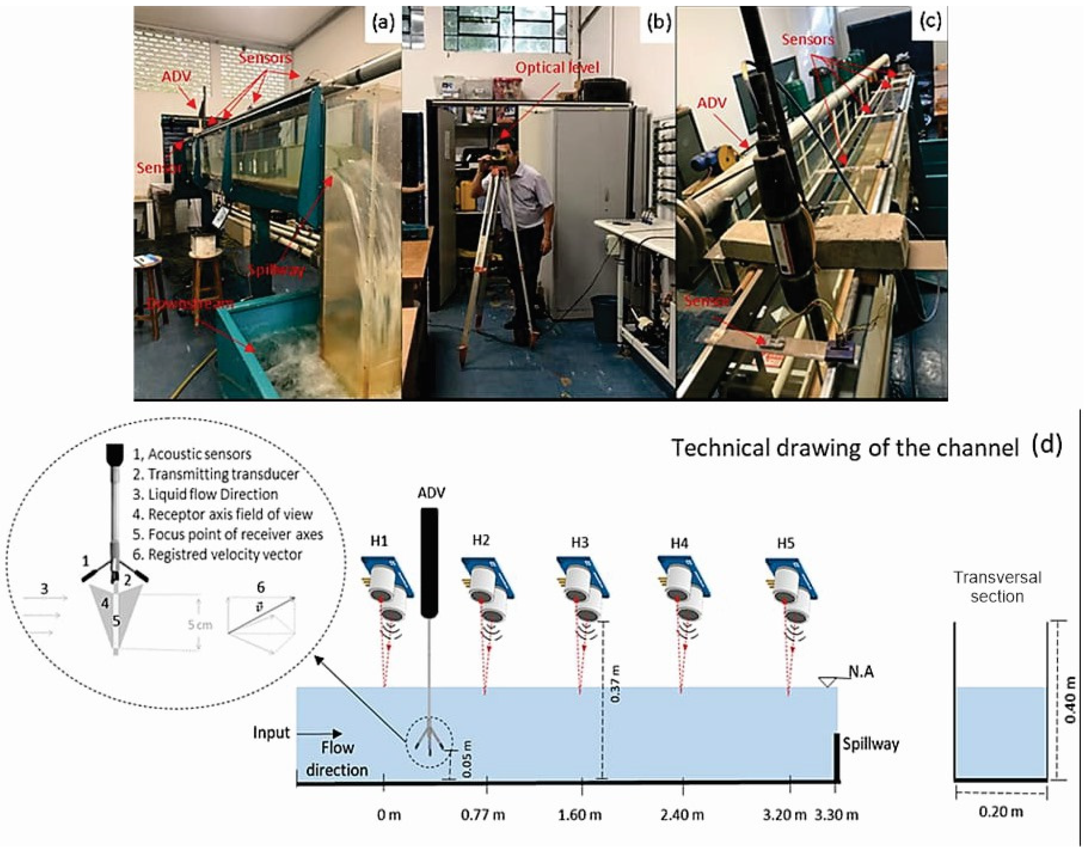
In this study, the slope was measured directly from the canal level measurement to have a process similar to that used in rivers, and only the Manning coefficient (n) was adjusted. The n adjustment process was performed manually for the EV1, resulting in a value of n = 0.011. This value is compatible with that found in the literature for very smooth surfaces [29], as is the case of the evaluated channel, which has glass sidewalls and an acrylic bottom.

The sensitivity analysis showed that discharge is the most sensitive parameter to Manning’s coefficient (n) and slope (So) changes. Height was the least sensitive parameter, with a seven times more minor percentage change than discharge (Figure 3).

Although the two parameters n and S_o have a minor proportional change compared to the two variables Q and H, the relationship between Q and S_o was much stronger than the others (Q/n, H/n, and H/So). This result indicates that discharge is significantly sensitive to topography, while height has minor sensitivity (Figure 3).

Events 1 and 4 differ in the height of the weir at the end of the channel, which affects the flow in the analysis section. Event 1 has less interference from the backwater effect, which implies a higher sensitivity of the roughness coefficient (n) to the flow. In Event 4, the velocities are lower, meaning lower energy losses, as reflected in the low sensitivity of both the flow and the height to the roughness coefficient (n). In determining flows through hydrodynamic simulations, topographic data are essential to ensure the reality of the results under all backwater conditions. The roughness coefficient (n) is necessary when the backwater effect in the section is lower, as the flow is more sensitive to this parameter under these conditions.

The quantitative metric results for the different events are presented in

Table 2. Summarizes the mean of values for the calibration and validation events.

EV1					EV2
Events	NSE	RMSE (m s−1 and m)	PBIAS (%)	ER (%)	Events	NSE	RMSE (m s−1 and m)	PBIAS (%)	ER (%)
Vel1	0.840	0.0669	0.44	9.73	Vel2	0.900	0.0473	−1.99	11.46
H2	0.958	0.00439	0.39	2.99	H2	0.981	0.00392	−0.47	1.70
H3	0.968	0.00392	−0.11	2.34	H3	0.992	0.00259	−0.01	1.16
H4	0.970	0.00392	−1.28	2.31	H4	0.979	0.00392	−1.47	1.76
H5	0.964	0.00392	−2.10	2.76	H5	0.981	0.00392	−1.61	1.83
EV3					EV4
Events	NSE	RMSE (m s−1 and m)	PBIAS (%)	ER (%)	Events	NSE	RMSE (m s−1 and m)	PBIAS (%)	ER (%)
Vel3	0.653	0.0826	−5.28	13.27	Vel4	0.912	0.0384	−1.00	7.69
H2	0.965	0.00392	2.27	3.59	H2	0.993	0.00238	−0.08	1.06
H3	0.960	0.00457	2.31	3.48	H3	0.995	0.00238	0.41	0.98
H4	0.934	0.00608	4.11	4.45	H4	0.983	0.00346	0.15	1.68
H5	0.948	0.00551	−3.42	4.00	H5	0.964	0.00521	−2.66	2.64

and

Table 3. Summary of observed and calculated means, standard deviations, root mean square error (RMSE), and root mean square error–the ratio of the standard deviation of observations (RMSE–RSR), for calibration and validation events.

Events	MEANObs (m s−1 and m)	SDObs	MEANCal (m s−1 and m)	SDCal	SDObs/2	RMSE (m s−1 and m)	RMSE–RSR (RMSE/SDObs)
EV1
Vel1	0.523	0.167	0.520	0.150	0.084	0.0669	0.400
H2	0.122	0.021	0.122	0.023	0.011	0.00439	0.206
H3	0.128	0.022	0.128	0.004	0.011	0.00392	0.180
H4	0.131	0.023	0.132	0.024	0.011	0.00392	0.171
H5	0.133	0.024	0.136	0.024	0.012	0.00392	0.165
EV2
Vel2	0.374	0.150	0.382	0.143	0.075	0.0473	0.316
H2	0.177	0.029	0.178	0.029	0.015	0.00392	0.135
H3	0.183	0.029	0.183	0.030	0.015	0.00259	0.089
H4	0.184	0.028	0.187	0.030	0.014	0.00392	0.139
H5	0.188	0.029	0.191	0.030	0.015	0.00392	0.133
EV3
Vel3	0.439	0.140	0.463	0.137	0.070	0.0826	0.589
H2	0.103	0.022	0.101	0.023	0.011	0.00392	0.177
H3	0.111	0.023	0.109	0.024	0.011	0.00457	0.199
H4	0.122	0.024	0.117	0.024	0.012	0.00608	0.256
H5	0.120	0.024	0.124	0.025	0.012	0.00551	0.228
EV4
Vel4	0.367	0.129	0.371	0.130	0.065	0.0384	0.297
H2	0.161	0.029	0.161	0.028	0.014	0.00238	0.083
H3	0.169	0.028	0.169	0.028	0.014	0.00238	0.087
H4	0.176	0.026	0.176	0.028	0.013	0.00346	0.132
H5	0.178	0.027	0.183	0.028	0.014	0.00521	0.191

and Figure 4 and Figure 5.

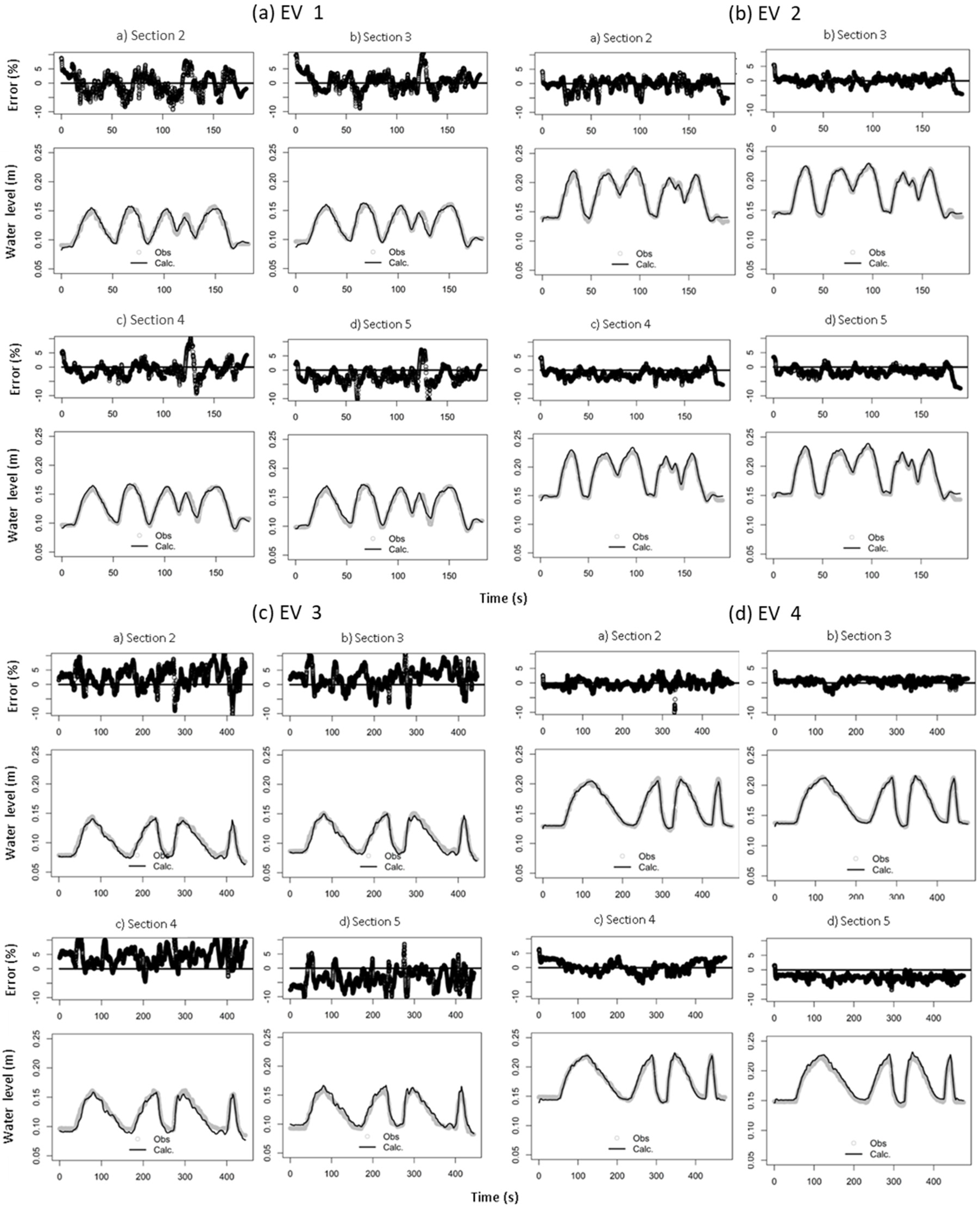
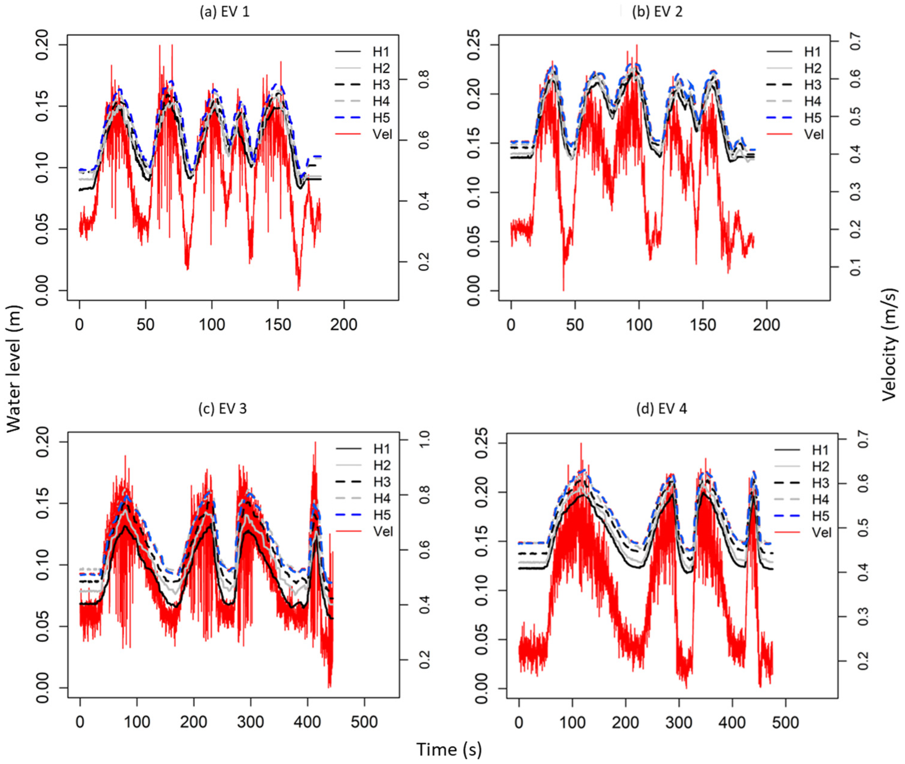
The results of the metrics indicate that the model simulated the water level trends very well for all the events, with the average NSE values ranging from 0.958 to 0.995 (Table 2), a result corroborated by the graphs (Figure 5). The errors were more significant for the velocities, with the average NSE values ranging from 0.653 to 0.912 (Table 2), with greater dispersion of the values between the curves in the graphs (Figure 4). This is mainly due to the diffusion of the measured velocity data, as the ADV can measure the degree of turbulence in the flow.

EV2 and EV4 had higher water levels and lower velocities (0.20 m–0.38 m s⁻¹), while EV1 and EV3 had lower water levels and higher velocities (0.15 m and 0.49 m s⁻¹) (Table 2). EV2 and EV4 had higher average NSE values (0.983 and 0.984) for the water levels than EV1 and EV3 (NSE 0.965 and 0.952), indicating a better model simulation. The same trend occurred for the velocities, with NSE values of 0.900 and 0.912 for EV2 and EV4, and 0.840 and 0.653 for EV1 and EV3. This is because the turbulence is generally lower in more profound and slower flows, which makes measurements easier. In summary, turbulence can cause readings with greater dispersion, which one-dimensional models do not consider. All the events evaluated were subcritical, as the ADV can only be used in water depths greater than 5 cm.

A simple and manual model adjustment produced good results consistent with the channel’s physical characteristics. Therefore, the model can be used in situations with limited velocity data, using only water level data and a topographic survey that can represent the slope of the channel bed.

When the metrics used to evaluate the model, RMSE, RMSE–RSR, PBIAS, and ER (Table 3), were analyzed, it was observed that they produced results similar to the NSE. EV1 and EV3 showed poorer simulation quality, while EV2 and EV4 showed better quality. The slope was unnecessary, as EV1 and EV3 had similar depths, and the spillway drowned the flow in the EV2 and EV4 events.

Table 3 shows that the model performed well in terms of the calibration and validation for the water levels and velocities, with average RMSEs less than half the standard deviation of the observations, except for the EV3 velocity, which was overestimated by ≈ 0.025 m s⁻¹. The overestimation of the EV3 velocity is evident when comparing the observed and calculated mean velocity values, which were higher than 5% of the observed mean.

The model performed well for the residual variation of the water levels and velocities in the calibration and validation, with an average RMSE–RSR less than 0.50, except for the EV3 velocity, which was considered good, with an RMSE–RSR of 0.59 (Table 3). These values indicate that the model’s performance for the residual variation of the levels and velocities was excellent most of the time, since 0.50 is considered a more rigorous classification [27].

The model also performed well, with a mean PBIAS of less than ±10% for the calibration and validation (Table 3). The PBIAS values ranged from −2.10% to 0.40% for the water levels and −3.40% to 4.10% for the velocities. Most of the time, the average of the calculated values was higher than the observed values.

According to Table 3, the model performed excellently for the levels, with a mean ER of less than 5% for the calibration and validation. The performance for the velocities was lower, with a mean ER of greater than 5% (calibration = 9.73% and validation 7.69–13.27%). The greater variation for the velocities is due to the variability of the ADV measurements, which can measure 3D flow and determine turbulence.

Graphically (Figure 4 and Figure 5), it is observed that the calculated values closely followed the observed values in the calibration (Figure 4a and Figure 5a) and validation (Figure 4b–d and Figure 5b–d), even for unfavorable flow conditions. This indicates that the model can simulate flow across the states examined. The model also reproduced the flow propagation, with peaks coinciding at the four observed points.

For the levels, the distributed ER was higher for EV1 and EV3 (Figure 4a,c), reaching 9.98%. The errors were smaller for EV2 and EV4 (Figure 4b,d), not exceeding 7.41%. The most significant errors occurred at the beginning of the simulation when the model was still warming up. The slightest errors occurred in the peak flow region, with higher observed water levels. The model did not show a trend of overestimation or underestimation, indicating that it has good predictability.

For the velocities (Figure 5), the errors increased as the velocity increased due to the increased turbulence. In Event 3, the velocity measurements at the first and second peaks exhibited discontinuous values compared to those observed in the other three events. The distributed ER was larger for all the events, but more than 85% of the errors were less than 20%, and more than 4% were less than 40%.

Therefore, the model presented excellent results for the trends of the water levels and velocities. From a more conservative perspective, it can be considered satisfactory. The good fits are evidenced by the statistical metrics, which agree with the graphical results.

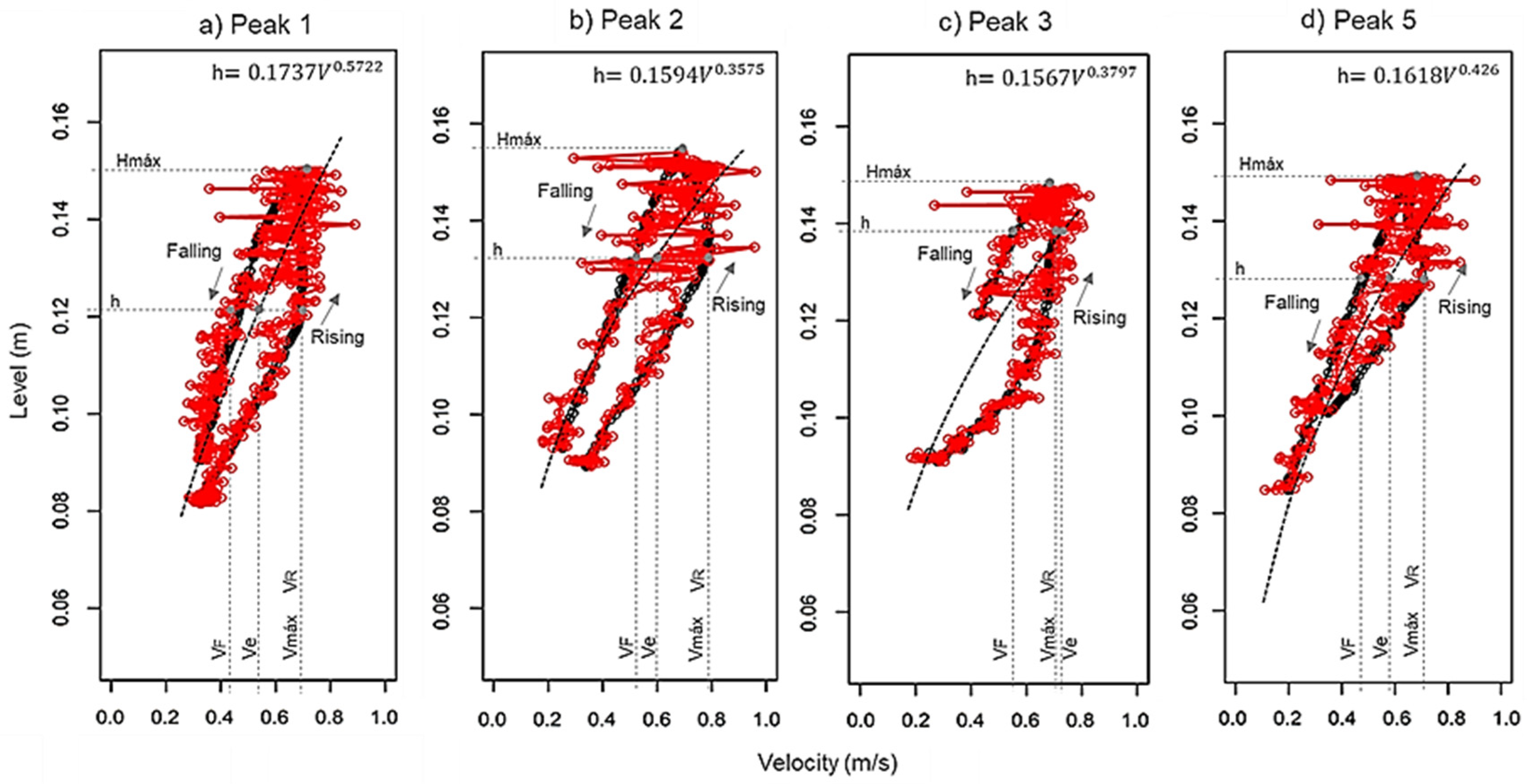
To evaluate the transient effect on the relationship between the velocity and level, speed and level data were compared by segment for the EV1 inlet section (Figure 6). The division of the event into segments was carried out by peak to isolate the effects of hysteresis and, thus, achieve a better visualization.

The loop-shaped rating curve displays two distinct curves, one for the flood rise and another for the recession. During the rising limb, the maximum discharge (Qmax) and maximum velocity (Vmax) of the flow coincide, but at a level (h) that differs from the maximum depth (Hmax). This divergence contrasts with the steady flows, where the relationship is linear and the Qmax or Vmax corresponds to the same point as Hmax on the Cartesian x-y-axis.

In transient flows, this deviation occurs due to the increase in the local and convective acceleration terms during the flood rise, resulting in an increase in the velocity and, consequently, the flow rate at that specific point. During the flood recession, the opposite occurs, resulting in a lower flow rate for the same water level h. Thus, in transient flows, the same depth, h, can correspond to two different flow rates, depending on whether the flood wave is rising or receding. In contrast, in uniform or steady permanent flows, the acceleration terms are disregarded or simplified in the statistical formulation, and therefore, they are represented by a single curve.

The existence of the hysteresis loop in the peaks 1, 2, 3, and 5 is confirmed in this way (Figure 6a–d). In these cases, the relationship between the water level and velocity is biunivocal, meaning that for the same water level (h), there are two distinct values of velocities (VF and VR). This phenomenon, known as hysteresis, indicates that the hydrodynamic model accurately represents this behavior. This assertion is supported by traditional rating curves represented by the solid black lines for steady or stable flow. These curves exhibit a one-to-one relationship between the water level (h) and velocity (Ve).

For peak 1 (Figure 6a), the maximum velocity on the rising limb (VR) was 0.70 m s⁻¹ (0.017 m³ s⁻¹) at a level of 0.121 m. At the same level, the recession limb (VF) velocity was 0.42 m s⁻¹ (0.010 m³ s⁻¹). The difference between the VR and VF was 0.28 m s⁻¹ (0.007 m³ s⁻¹), corresponding to 40%. The traditional rating curve underestimates the VR by 23% and overestimates the VF by 29%.

Peaks 2, 3, and 5 (Figure 6b–d) exhibited the same behavior as peak 1, with differences between the VR and VF velocities of, respectively, 34% (0.27 m s⁻¹ and 0.007 m³ s⁻¹), 20% (0.14 m s⁻¹ and 0.004 m³ s⁻¹), and 32% (0.23 m s⁻¹ (0.006 m³ s⁻¹). The hydrographs of the transient flow variables do not occur simultaneously as they do for permanent flow. This is because the maximum levels (H_max) do not correspond to the maximum velocities (V_max) and, consequently, to the maximum discharges (Q_max), which tend to occur before these levels are reached.

Also, when the measured velocities (Ve) were compared to the predicted velocities based on the rating curves (VR) and full-flow velocities (VF) for peaks 2, 3, and 5, it was found that, for peak 2, the Ve was underestimated by −0.19 m s⁻¹ (−0.005 m³ s⁻¹) (24%) relative to the VR and overestimated by 0.08 m s⁻¹ (0.002 m³ s⁻¹) (15%) to the VF. For peak 3, the Ve was overestimated by 0.02 m s⁻¹ (0.001 m³ s⁻¹) (3%) in both the rising and receding limbs of the flood wave relative to the VR and by 0.16 m s⁻¹ (0.004 m³ s⁻¹) (28%) to the VF. For peak 5, the Ve was underestimated by −0.13 m s⁻¹ (−0.003 m³ s⁻¹) (18%) relative to the VR and overestimated by 0.1 m s⁻¹ (0.003 m³ s⁻¹) (21%) to the VF. For peak 4, analyzing the hysteresis behavior was impossible due to the relatively small wave amplitude, between 0.10 and 0.14 m, which was not considered.

It was also found that, even for a specific level, the velocity values can vary from event to event. For example, for the peaks at the level of 0.14 m, the observed deviations were 0.69, 0.78, 0.70, and 0.63 m s⁻¹ in the rising limb and 0.58, 0.55, 0.58, and 0.58 m s⁻¹ in the receding stem. The mean of the deviations found was 0.70 m s⁻¹ (0.020 m³ s⁻¹) for the rising limb and 0.57 m s⁻¹ (0.016 m³ s⁻¹) for the receding limb.

The deviations found are consistent with the physical concept of hysteresis, which is influenced by the system’s memory effect [30,31]. In the case studied, the flow remaining time may be one of the factors influencing the observed deviations. These deviations can be larger between the middle of the rise and the depletion curves, where the hysteresis width is greater. Therefore, these deviations may be even more significant for flows in natural channels due to friction between the channel walls and the bottom.

4. Discussion

The article focuses on the hydrodynamic simulation of transient flow in a rectangular channel based on continuous data concerning the water levels and velocities for flow estimation. The hydrodynamic model was implemented and calibrated against the water level and velocity data obtained from a laboratory experiment.

This article presents a relevant contribution by assessing the measurement of continuous velocities using high-frequency acoustic Doppler velocimeters (ADVs) in transient flows to validate the results obtained from simulations with a hydrodynamic model that employs only the water levels as upstream boundary conditions. While hydrodynamic concepts are well-known and discussed, there is a lack of studies evaluating the velocity changes during rapid flow transitions, where typically only point data have been employed.

The results indicated that the hydrodynamic model exhibits a more monotonic behavior in terms of the water levels and velocities, as it does not account for local turbulence in its formulation. Local turbulence is responsible for small fluctuations in the water surface, manifested as noise. These noises can be mitigated by more sensitive sensors or filtering techniques.

The instantaneous variations in the velocity values were highly pronounced. The acoustic Doppler velocimeter (ADV) employed can measure velocity in all three spatial axes. Consequently, the determined value represents the velocity vector aligned with the flow, and due to its high spatial resolution (25 Hz), it can capture information on turbulent changes, which were found to be substantial during the assessed events. However, when evaluating the velocity profiles themselves, they appear to be close and fluctuate within the range of values calculated by the models for over 90% of the simulated time. This suggests two key observations: firstly, the hydrodynamic model, as currently developed, is incapable of simulating turbulent flow changes within intervals shorter than 1 s. Nevertheless, it effectively represents the average velocity values.

Some studies have conducted velocity measurements in turbulent flows but employed high time intervals. For instance, [3,19,20] worked with point measurements of the discharge, capturing only a single point per assessed event and not tracking the rising and falling phases of the hydrograph. These intervals may surpass the time scale of the velocity fluctuations, potentially losing crucial information about the flow turbulence. In our case, applying a data filter to the velocities might reduce these fluctuations, but it could also result in the loss of significant details, such as the chaotic nature of the actual flow, which deviates from the mean values obtained in the model. They acknowledge these modeling limitations and remember that preserving the chaotic aspects of natural flow is essential for comprehensive understanding.

However, the model successfully replicated the flow behavior at both levels and velocities, employing the channel’s inlet level as a boundary condition. As measuring the water level is more straightforward and cost-effective than measuring the velocity, its measurement, along with a hydrodynamic model, has been demonstrated to be efficient and supported by the velocimeter measurements.

The observed hysteresis effect was significant, indicating that using the rating curve as a method for determining flow in transient flow conditions is unsuitable. Although the simulations were conducted in a small-scale channel with pronounced temporal variations in flow, both the measured and calculated values demonstrate that the errors in flow estimates using the rating curve can be substantial. In our conditions, the errors reached up to 40%. This underscores the need for a more comprehensive study to assess the limitations of the rating curve as a source of flow data in rivers.

The ultrasonic sensors are promising water level measurement and flow estimation tools, as they demonstrate good accuracy, low cost, and quick and straightforward data acquisition. Furthermore, using open-source code enables control over the entire process and real-time visualization of all the variables returned by the sensor. Expanding this application to field conditions, such as rivers, with the development of stream gauges, represents a forthcoming challenge, as it would make data acquisition accessible to a broader audience.

In general, the implications of the study results indicate that the implemented model can accurately estimate discharge rates, making it suitable for water resources management. The findings can also contribute to a better understanding of the behavior of transient flows and aid in developing practical applications for simulating flows in natural channels. However, it is crucial to emphasize that the study was conducted in a rectangular channel with controlled flow conditions. Additional investigations in natural channels are required to validate the study results under real-world conditions.

5. Conclusions

We investigated the flow and velocity estimates generated from implementing a hydrodynamic model that utilizes only continuous water level information measured using ultrasonic sensors as the upstream boundary conditions for transient flow. The results demonstrated that the sensors are a reliable source for acquiring water level data, and the model could accurately estimate the flows and velocities for turbulent flows influenced by hysteresis effects. This accuracy is contingent upon conducting a thorough topographic survey to define the channel bed slope and accurately estimating the Manning coefficient during calibration. These findings align with the initial objective proposed in this article.

The calculated discharge and velocity showed a maximum variation of 40% for the same level compared to those estimated with the rating curve method. Thus, the results showed that hysteresis is an essential factor affecting the estimated discharge values in natural watercourses.

The results’ implications are significant, as the implemented model has proven capable of accurately estimating flow rates, enabling its use for water resources management and the simulation of flows in natural channels. However, it is emphasized that further studies under actual conditions, particularly in natural channels, are necessary to validate the results thoroughly.

The objective functions (FOs) and the general performance classifications used proved suitable for assessing the model predictions, although no studies were found recommending or not recommending their applications for evaluating hydrodynamic models. The Kling–Gupta efficiency (KGE), proposed by [32] and modified by [33], although commonly employed for calibration in hydrology, was not utilized in this study as the focus was on isolated events without base flow periods. In such cases, the NSE and RMSE are more suitable performance indicators. However, if the study had assessed a continuous hydrological model, we acknowledge that the KGE would be a better option.

We recommend considering the application of a filter for the velocities in future works to reduce the noise generated in the data acquisition process. For future studies, we suggest fixing the water level, altering the Manning coefficient by 0.1 and 0.5, respectively, and evaluating the Nash–Sutcliffe efficiency (NSE) values. This approach allows for assessing the sensitivity of the Manning coefficient to the water levels and flows for comparison purposes despite acknowledging that the flows are highly sensitive to the Manning coefficient variations, as explained here.

Moreover, assessing the continuous velocity measurements in transient flows and discussing the limitations of the hydrodynamic model contribute to advancing knowledge in the field, providing crucial insights for improving future research and practical applications. In summary, the results of this study offer relevant support for developing more precise and reliable methodologies for estimating the flows and velocities in natural channels, thereby enhancing the management of water resources and the safety of hydraulic infrastructure projects by reducing uncertainties in estimated flows.