The Potential of Isotopic Tracers for Precise and Environmentally Clean Stream Discharge Measurements

Abstract

Accurate discharge measurement is mandatory for any hydrological study. While the “velocity” measurement method is adapted to laminar flows, the “dilution” method is more appropriate for turbulent streams. As most low-gradient streams worldwide are neither laminar nor turbulent, a methodological gap appears. In this study, we demonstrate that the application of the “dilution” method to a low-gradient small stream gives very satisfactory results in addition to revealing surface/subsurface processes. A variety of chemical and isotopic tracers were injected into the stream (anions, fluorescent dyes, and chloride and hydrogen isotopes). We report the first use of ³⁷Cl for stream discharge measurement and show that ³⁷Cl and ²H can be reliably used as quantitative tracers. Discharge uncertainty calculations show that deuterium is the most accurate tracer method used. We also compare the differences in the tailing part of the restitution curves of tracers and investigate the role of transient surface and hyporheic zones in solute transport in light of a simple transport modelling approach. We conclude that isotopic tracers can be used as “environmentally friendly” tracers for discrete stream discharge measurements and that the application of multi-tracers tests in rivers opens the path to a better understanding of surface–subsurface interaction processes.

1. Introduction

Surface waters discharge measurement is a fundamental aspect of any hydrological and hydrogeological study. Indeed, accurate and precise stream discharge measurement is critical for water resource monitoring; water budget computation; hydraulic infrastructure design, such as weirs, culverts and artificial channels; flood monitoring and forecasting; and groundwater inflows calculations [1,2,3,4]. Different field approaches can be used to determine stream discharge [2,5]. One of the most used techniques is based on the use of current meters. The discharge is deducted by integrating the flow velocity distribution over a river cross-section area. Discharge measurement uncertainties using current meters largely depends on the velocity measure uncertainties and is usually between 2% and 20%, depending on measurement conditions [2,6,7]. This technique is best suited for open channels with near-laminar flow. Indeed, the representativeness of velocity measurements is very limited in turbulent streams [8] or in the presence of dead storage zones and backwaters [9]. The second technique is the so-called “gauging by tracer dilution” method. This technique consists of injecting a known mass of tracer upstream and measuring its complete restitution over time downstream [5]. Several key hypotheses must be verified: (i) complete dissolution and conservation of the tracer, (ii) homogeneity of tracer concentration across the river section at the measurement point downstream (ensured by transverse and vertical dispersion), and (iii) the discharge must be under a permanent regime during the entire experiment duration [8]. The use of the tracer dilution technique is especially appropriate in shallow, turbulent streams where hydrodynamic dispersion ensures a fast tracer homogenization, i.e., in contexts not suitable for traditional current meters.

The main limitation of the “dilution” technique is the presence of transient storage zones, both at the surface and in the subsurface. Indeed, it is now widely accepted that streams exchange intimately with surrounding groundwater bodies in a variety of climates [10,11,12,13,14], especially in temperate, wet climates [14]. Groundwater and surface waters act as a continuum, and exchange in the hyporheic zone, i.e., the portion of sediments surrounding the stream that is permeated with stream water, is significant [15]. Transport in the hyporheic zone is thus much slower than in the main stream channel, allowing biological and geochemical processes to occur [16]. In addition, the transport in the hyporheic zone, as well as in surface transient storage zones, results in a tailing effect in restitution curves of artificial tracer injection, which might limit the “dilution” method [1]. Exchanges with the hyporheic zone are mainly controlled by streambed porosity and permeability. They are known to be mainly advective but can be controlled by diffusion in the presence of fine streambed sediments, such as clays, in calm streams [15]. Hyporheic exchanges are typically modelled using the classical advection dispersion equation (ADE) to which a sink term representing the subsurface exchanges with the stream is added [15,17,18,19,20]. Then, hyporheic flow represents the portion of stream water that is transported through the hyporheic zone before returning to the stream. In hydrological modelling, model parameters are calibrated against field data of tracer tests, often thanks to fluorescent dyes and salts tracers. Most low-gradient small streams worldwide consist of a succession of small pools and riffles, with very contrasted flow velocities, important streambed macro-topography, and the presence of transient storage zones. The flow in these rivers is not exclusively laminar or exclusively turbulent, which indicates a gap in streamflow measurement methodology.

Globally, anthropogenic activities have various negative impacts on stream quality, mainly resulting in biodiversity loss and eutrophication issues [21,22]. In addition, it is well known that groundwater pumping can decrease water levels in rivers [23]. In this context, the application of the “dilution” method through injection of salts (e.g., NaCl) can be problematic for aquatic ecosystems [24] and in rivers exploited for drinking water because their use will temporarily damage the stream quality. It is thus relevant to search for more environmentally friendly tracers for stream discharge measurements. For a given river discharge, the quantity of tracer has to be minimized but will depend on the initial stream concentration and the accuracy of the measurement. Chemical elements that are naturally found in small quantities and that can be analysed with a very high accuracy can therefore be injected in sufficiently small quantities to minimize their impact on the environment. While less used, “heavy” natural stable isotopes that are naturally present in (very) small amounts can be measured with a high precision using mass spectrometry. Hence, deuterium (²H) is an ideal tracer of the water molecule since it is naturally bound to it and is fully conservative. It has already been used in many artificial tracer injections, especially in various groundwaters studies [25] but not yet for river discharge measurements. Rarely used, chloride isotopes are interesting tracers because of the high solubility of chlorine and the fact that it is conservative in aquatic systems [26]. Chlorine has two common stable isotopes, ³⁵Cl and ³⁷Cl, and high-accuracy mass spectrometry measurements are very promising for environmental studies. The application of these “cleaner” isotopic tracers opens new perspectives to the understanding of environmental processes.

The objectives of this study are multiple: (i) to compare both the velocity and dilution methods for discharge measurements of a small stream, (ii) to assess the potential of isotopic tracers for more environmentally friendly discharge measurements, and (iii) to document surface–subsurface processes in the light of a multi-tracer approach. To complete these objectives, a diverse array of tracers, including electrolytes (NaBr, ³⁷Cl-enriched salt) conservative anions (bromide [Br⁻] and chloride [Cl⁻]), stable isotopes (deuterium [²H] and chlorine [³⁷Cl]) and fluorescent dyes (uranine, tinopal) were injected into a small stream (Ruisseau Rousse, Québec, Canada) and analysed. We compare two approaches for stream discharge determination and hypothesize that the “dilution” method can be employed with satisfactory results for low-gradient small streams. Finally, we compare the tailing effect of tinopal, ²H, ³⁷Cl and Br⁻ in restitution curves to assess the exchange processes between the stream main channel and transient storage zones. The simultaneous injection of tracers having different chemical and physical (size) properties enabled us to gain a better understanding of these interactions/processes.

2. Materials and Methods

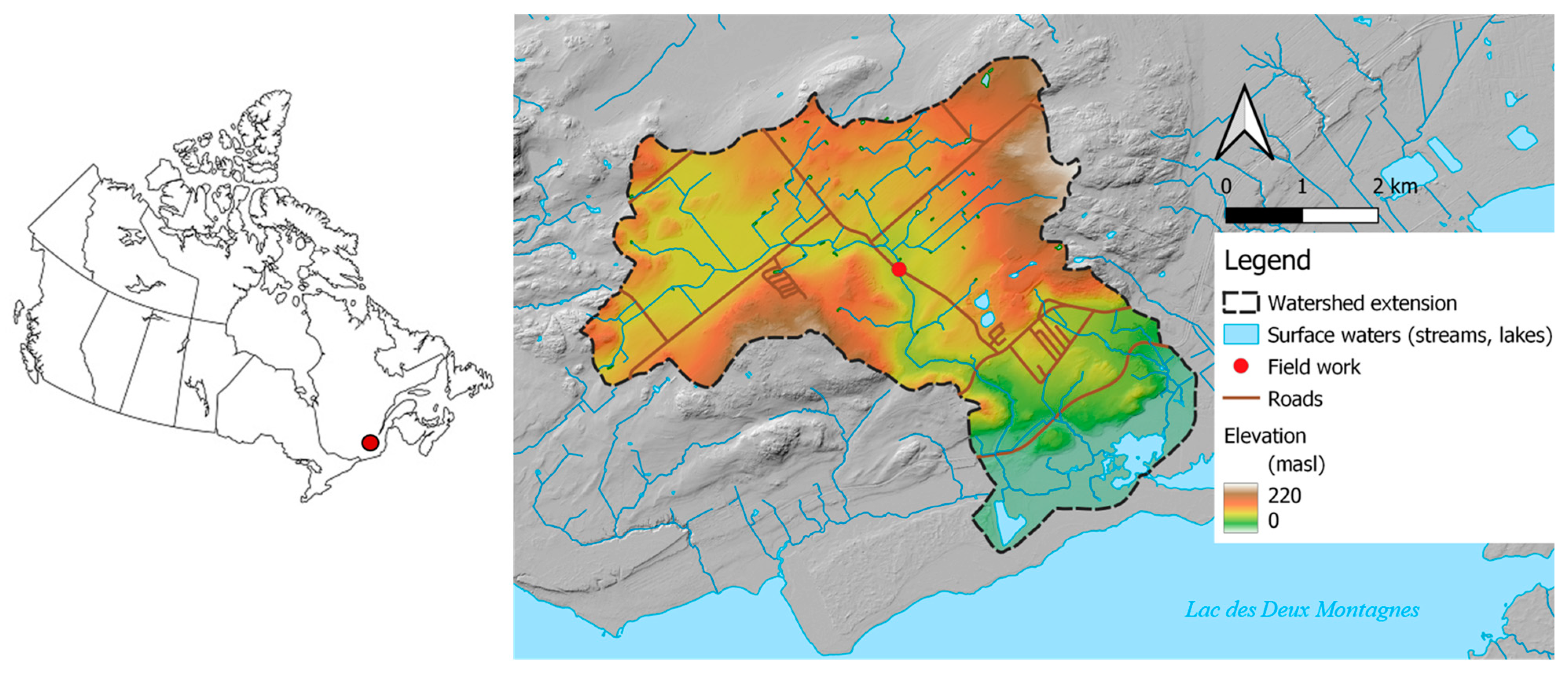
2.1. Description of the Field Site

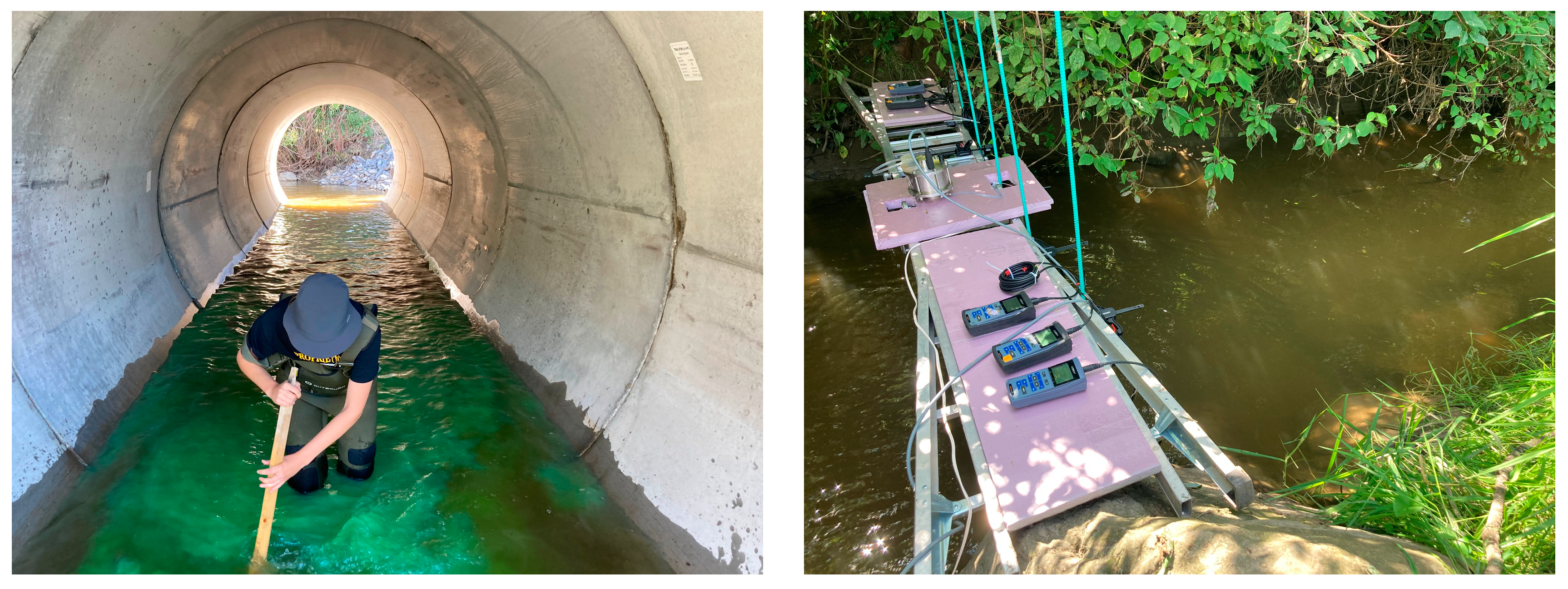
Field work occurred in Oka, Québec, Canada in August 2022 in a small stream under baseflow conditions (coordinates: 45°30′15.8″ N/74°02′45.9″ W—see Figure 1 below) on a sunny day without any precipitation. In addition, the last precipitation event occurred 8 days before the test, roughly 4 times the recession time of this small river. The basement geology of the watershed consists of intrusive plutonic rocks (charnockite, mangerite) from the Precambrian age and Mesozoic carbonatite. It is covered by quaternary glacio-marine deposits (silts to gravel sands) that shelter the alluvial aquifer sustaining the river [27]. The local climate is continental humid, characterized by long, cold, and snowy winters and hot and wet summers. The watershed is mainly cultivated, but its southern part is occupied by the Parc National d’Oka, a protected natural area. The stream, called Ruisseau Rousse, drains the watershed and flows to the Lac des Deux Montagnes before ultimately joining the St. Lawrence River.

The studied river transect extends 105 metres from the injection site (IS) to the restitution site (RS) (Figure 2). Similar to numerous streams in intermediate gradient plains, it is characterized by a succession of pools and small riffles with very contrasted flow velocities, river widths, and river depths. The average river width was estimated to be 2 m (2.6 m at the studied cross-section), with the maximal cross-sectional depth varying between 10 and 60 cm.

2.2. Field Work

The solution used for the tracing experiment contained approximately 20 L of river water to which a variety of tracers was added: 535.13 ± 0.01 g of Cl⁻ with a δ³⁷Cl value of +2.18‰ ± 0.03 vs. SMOC (supplier: BioBasic, Markham, ON, Canada), 788.60 ± 0.01 g of Br⁻ (supplier: Fischer Scientific, Ottawa, ON, Canada), 403.09 ± 0.20 g of ²H as deuterated water ²H₂O (supplier: Isowater, Collingwood, ON, Canada), 2.42 ± 0.01 g of uranine, and 16.50 ± 0.01 g of tinopal (supplier: ThermoFischer, Waltham, MA, USA). The sample was placed in a sealed bucket until the salts dissolved completely, which took a few minutes. The total dissolved solids (TDS) of the mixture was 126.4 g/L. It was then injected instantaneously at IS. We ensured tracer homogeneity across the river width by manually fanning the river at IS shortly after injection (Figure 2). The injected volume has no effect regarding the total stream discharge.

Stream water velocity was measured using a SonTek FlowTracker at RS in 55 points across the river section to assess its distribution with a high spatial resolution, minutes before the injection occurred. At RS, a total of five field multimeters (WTW) and 2 Solinst^® LTC loggers were used to monitor the distribution of salt tracers (using electrical conductivity) across the section at a time step of 5 s. All of the equipment was calibrated against a 1413 µS/cm standard in the morning of the field experiment. The mean uncertainty in electrical conductivity measurements was reported to be 1.1% of the measured value. Water fluorescence was monitored at RS in the centre of the stream (green dot in Figure 3), at a time step of 15 s using a field fluorometer (Tetraedre GGUN FL-30). Samples for anions (Cl⁻, Br⁻) and isotopic compositions (²H, ³⁷Cl) were taken in the centre of stream at two points (Fluo. and WTW3) at 10 and 30 cm of depth (distance = 120 cm from the left bank, see Figure 3) in 250 mL HDPE bottles. The first discrete samples were taken every 2 min, and the time interval of sampling was progressively reduced up to 30 s when approaching to the arrival of the peak of tracer. It was then increased up to 5 min during the tailing part.

2.3. Analytical Methods

Since discharge computation requires concentration data, the electrical conductivity signal was converted into an added salts concentration time series. To do so, a sample of the river water was obtained prior to the injection (1L in HDPE bottle). Salts were carefully added in the same proportion as the injection mix (i.e., 40.4% of NaBr and 59.6% of ³⁷Cl-enriched salt) and progressively dissolved, and the relationship between electrical conductivity and added dissolved salts was assessed for each field probe. The field fluorometer was calibrated at the laboratory on the day before the tracing experiment using distilled water to which uranine and tinopal were added in known quantities (7 points ranging from 0 to 160 ppb for uranine and 10 points ranging from 0 to 1300 ppb for tinopal). Anion (chloride, bromide) analyses were performed using liquid ion chromatography at the Université du Québecà Montréal, QC, Canada (Geotop-UQAM lab).

Deuterium analyses were performed at the Geotop Light Stable Isotope Geochemistry Laboratory at UQAM. Exactly 200 µL of sample water was pipetted in a 3 mL vial containing a hydrophobic platinum catalyst (Hokko beads). The vials were then closed with a septum cap, transferred to a 40 °C heated rack, and left to equilibrate for 4 h. The equilibrated samples were analysed using a dual inlet ratio mass spectrometer (Micromass Isoprime IRMS coupled to an AquaPrep system). Four in-house standards were used to normalize the results on the VSMOW-SLAP scale (standard 1: δ²H = −99.45 ± 0.56‰ vs. VSMOW/standard 2: δ²H = +118.5 ± 4.4‰ vs. VSMOW/standard 3: δ²H = +323.5 ± 5.1‰ vs. VSMOW/standard 4: δ²H = +740.2 ± 3.2‰ vs. VSMOW). Chloride isotopes analyses were performed at Institut de Physique du Globe (IPGP) in Paris, France, using the AgCl-CH₃Cl method [28,29,30]. The chloride isotope compositions of the samples were measured using a gas source dual inlet isotope ratio mass spectrometer (Delta V from ThermoFisher) with ionizing CH₃Cl gas. The results are reported as the δ³⁷Cl vs. SMOC (standard mean ocean chloride). The relative contents of ²H and ³⁷Cl in stream water are expressed as δ-values, representing their deviation (in per mil) to the international standards of VSMOW (Vienna Standard Mean Ocean Water) for ²H (Equation (1)) and SMOC (standard mean ocean chloride) for ³⁷Cl (Equation (2)):

$${\mathsf{\delta }}^2\mathrm{H}=\left(\frac{{\left(\frac{{}^2\mathrm{H}}{{}^1\mathrm{H}}\right)}_{\mathrm{sample}}}{{\left(\frac{{}^2\mathrm{H}}{{}^1\mathrm{H}}\right)}_{\mathrm{VSMOW}}}-1\right){10}^3$$

(1)

$${\mathsf{\delta }}^{37}\mathrm{Cl}=\left(\frac{{\left(\frac{{}^{37}\mathrm{CI}}{{}^{35}\mathrm{CI}}\right)}_{\mathrm{sample}}}{{\left(\frac{{}^{37}\mathrm{CI}}{{}^{35}\mathrm{CI}}\right)}_{\mathrm{SMOC}}}-1\right){10}^3$$

(2)

where (²H/¹H)_VSMOW = 1.5575 × 10⁻⁶ and (³⁷Cl/³⁵Cl)_SMOC = 0.324 are the reference abundancy ratios for deuterium and chlorine-37, respectively [26]. Here, typical uncertainties (1σ) in the measurements of δ²H are of the order of ±1–2‰. Concerning δ ³⁷Cl, the external reproducibility of the Atlantique 2 seawater chloride reference was ±0.025‰ (1σ, n = 12).

The raw field data for all the tracers can be found as Supplementary Material (Excel spreadsheet S1).

2.4. Data Interpretation

Traditionally, when using a current meter, the discharge is deducted by integrating the flow velocity distribution over the whole river cross-section area:

$$\mathrm{Q}=\underset{\mathrm{A}}{\overset{}{\iint }}\mathrm{v}\left(\mathrm{x},\mathrm{y}\right)\mathrm{dxdy}$$

(3)

where Q is the stream discharge [L³T⁻¹], and v the water velocity field [LT⁻¹] that is a function of width (x—[L]) and depth (y—[L]). The variables x and y are used to define the river cross-section area, A.

Using the “dilution” method requires verification of the following hypotheses: (i) complete dissolution and conservation of the tracer, (ii) homogeneity of tracer concentration across the river section (ensured by transverse and vertical dispersion), and (iii) stream discharge under a permanent regime during the entire experiment duration [8]. When such conditions are met, the discharge is computed according to the following formula [1,25]:

$$\mathrm{Q}=\frac{{\mathrm{M}}_{\mathrm{tracer}}}{{\int }_0^{\mathrm{T}}\mathrm{C}\left(\mathrm{t}\right)\mathrm{dt}}$$

(4)

where M_tracer is the mass of tracer that is injected [M], and C(t) is the added tracer concentration at time t [ML⁻³]. The time t = 0 corresponds to the time of injection, while T is the total duration of the experiment. Discharge measurements using the “dilution” method can only be overestimated if one or more of the three assumptions are not met. Usually, the denominator is calculated using a simple numerical integration scheme, such as that noted in the following:

$${\int }_0^{\mathrm{T}}\mathrm{C}\left(\mathrm{t}\right)\mathrm{dt}=\frac{1}{2}\sum _{\mathrm{i}=1}^{\mathrm{N}-1}\left({\mathrm{C}}_{\mathrm{i}+1}+{\mathrm{C}}_{\mathrm{i}}\right)\left({\mathrm{t}}_{\mathrm{i}+1}-{\mathrm{t}}_{\mathrm{i}}\right)$$

(5)

where i refers to the i^th concentration measurement of the tracer (at time t_i), and N indicates the total number of measurements. Practically, the first sample (C₁) is taken at time 0, and the N^th sample (C_N) is taken at time T. Typically, when using field probes, the measurement timestep (ΔT) is constant, and Equation (5) is represented as follows:

$${\int }_0^{\mathrm{T}}\mathrm{C}\left(\mathrm{t}\right)\mathrm{dt}=\frac{1}{2}\Delta \mathrm{T}\sum _{\mathrm{i}=1}^{\mathrm{N}-1}\left({\mathrm{C}}_{\mathrm{i}+1}+{\mathrm{C}}_{\mathrm{i}}\right)$$

(6)

In addition, the uncertainty propagation calculation was performed based on Equations (4) and (5):

$$\Delta \mathrm{Q}=\left|\mathrm{Q}\right|\sqrt{{\left(\frac{\Delta {\mathrm{M}}_{\mathrm{tracer}}}{{\mathrm{M}}_{\mathrm{tracer}}}\right)}^2+\frac{\sum _{\mathrm{i}=1}^{\mathrm{n}-1}{\left({\mathrm{t}}_{\mathrm{i}+1}- {\mathrm{t}}_{\mathrm{i}}\right)}^2(\Delta {\mathrm{C}}_{\mathrm{i}+1}^2+\Delta {\mathrm{C}}_{\mathrm{i}}^2)}{{\left[\sum _{\mathrm{i}=1}^{\mathrm{n}-1}\left({\mathrm{t}}_{\mathrm{i}+1}- {\mathrm{t}}_{\mathrm{i}}\right)\left({\mathrm{C}}_{\mathrm{i}+1}+{\mathrm{C}}_{\mathrm{i}}\right)\right]}^2}}$$

(7)

where Δ refers to the measure uncertainty (1σ) in any given measurement. This assumes that there is no uncertainty in the timing of the measurement. Of note, in the case of a constant sampling timestep ΔT (e.g., electrical conductivity monitoring), Equation (7) simplifies to the following:

$$\Delta \mathrm{Q}=\left|\mathrm{Q}\right|\sqrt{{\left(\frac{\Delta {\mathrm{M}}_{\mathrm{tracer}}}{{\mathrm{M}}_{\mathrm{tracer}}}\right)}^2+\frac{\sum _{\mathrm{i}=1}^{\mathrm{n}-1}(\Delta {\mathrm{C}}_{\mathrm{i}+1}^2+\Delta {\mathrm{C}}_{\mathrm{i}}^2)}{{\left[\sum _{\mathrm{i}=1}^{\mathrm{n}-1}\left({\mathrm{C}}_{\mathrm{i}+1}+{\mathrm{C}}_{\mathrm{i}}\right)\right]}^2}}$$

(8)

Tracer experiments allow computation of stream discharge, but they also allow estimation of flow parameters, such as dispersion, velocity, and the influence of slower velocity zones. Here, flow parameters were determined by modelling the tracers’ restitution curves using a simple binary 1-D dispersion mixing model. A similar lumped parameter model approach was used to simulate the transport of an artificial tracer release in the Rhine river and is described in Leibundgut et al. [25]. Considering a conservative tracer, the classical 1-D lumped dispersion model can be expressed as follows [31]:

$$\mathrm{C}\left(\mathrm{t}\right)={\int }_{-\infty }^{\mathrm{t}}{\mathrm{C}}_{\mathrm{inj}}\left(\mathsf{\tau }\right)\mathrm{g}\left(\mathrm{t}-\mathsf{\tau }\right)\mathrm{d}\mathsf{\tau }$$

(9)

Here,

$$\mathrm{g}\left(\mathsf{\tau }\right)=\frac{\mathrm{v}}{\mathrm{x}\sqrt{4\mathsf{\pi }\frac{\mathrm{D}}{{\mathrm{x}}^2}\mathsf{\tau }}}{\mathrm{e}}^{\frac{{\left(1- \frac{\mathsf{\tau }\mathrm{v}}{\mathrm{x}}\right)}^2}{4\mathsf{\tau }\frac{\mathrm{D}}{{\mathrm{x}}^2}}}$$

(10)

Here, C is the tracer concentration over time [ML⁻³], D is the longitudinal dispersion parameter [L²T⁻¹], x the distance between the injection and measurement points [L], v the mean stream velocity [LT⁻¹], and C_inj is the injection function [ML⁻³]. Here, it is a Dirac-type function with a value of C₀ at t = 0.

In this binary mixing model approach, the measured tracer concentration was simulated by adding a second flow component representing the slower fraction:

$$\mathrm{C}\left(\mathrm{t}\right)={\mathrm{f}}_1{\int }_{-\infty }^{\mathrm{t}}{\mathrm{C}}_{\mathrm{inj}}\left(\mathsf{\tau }\right){\mathrm{g}}_1\left(\mathrm{t}-\mathsf{\tau }\right)\mathrm{d}\mathsf{\tau }+(1-{\mathrm{f}}_1){\int }_{-\infty }^{\mathrm{t}}{\mathrm{C}}_{\mathrm{inj}}\left(\mathsf{\tau }\right){\mathrm{g}}_2\left(\mathrm{t}-\mathsf{\tau }\right)\mathrm{dt}$$

(11)

The model was distributed over time and implemented in Excel (time step of 10 s). It was fitted with tracer restitution curves by minimising the normalized root mean square deviation defined as ${\mathsf{\chi }}^2=\sum \frac{{\left({\mathrm{C}}_{\mathrm{m}\mathrm{e}\mathrm{a}\mathrm{s}}-{\mathrm{C}}_{\mathrm{s}\mathrm{i}\mathrm{m}}\right)}^2}{{\mathrm{C}}_{\mathrm{m}\mathrm{e}\mathrm{a}\mathrm{s}}}$ (where C_meas is the measured value, C_sim is the simulated value). The parameters of the model were fitted using the restitution curves of ²H, ³⁷Cl, and Br⁻. The Excel spreadsheet containing the model as well as its documentation can be downloaded as Supplementary Materials (Excel spreadsheet S2 and Text file S1 respectively).

3. Results and Discussion

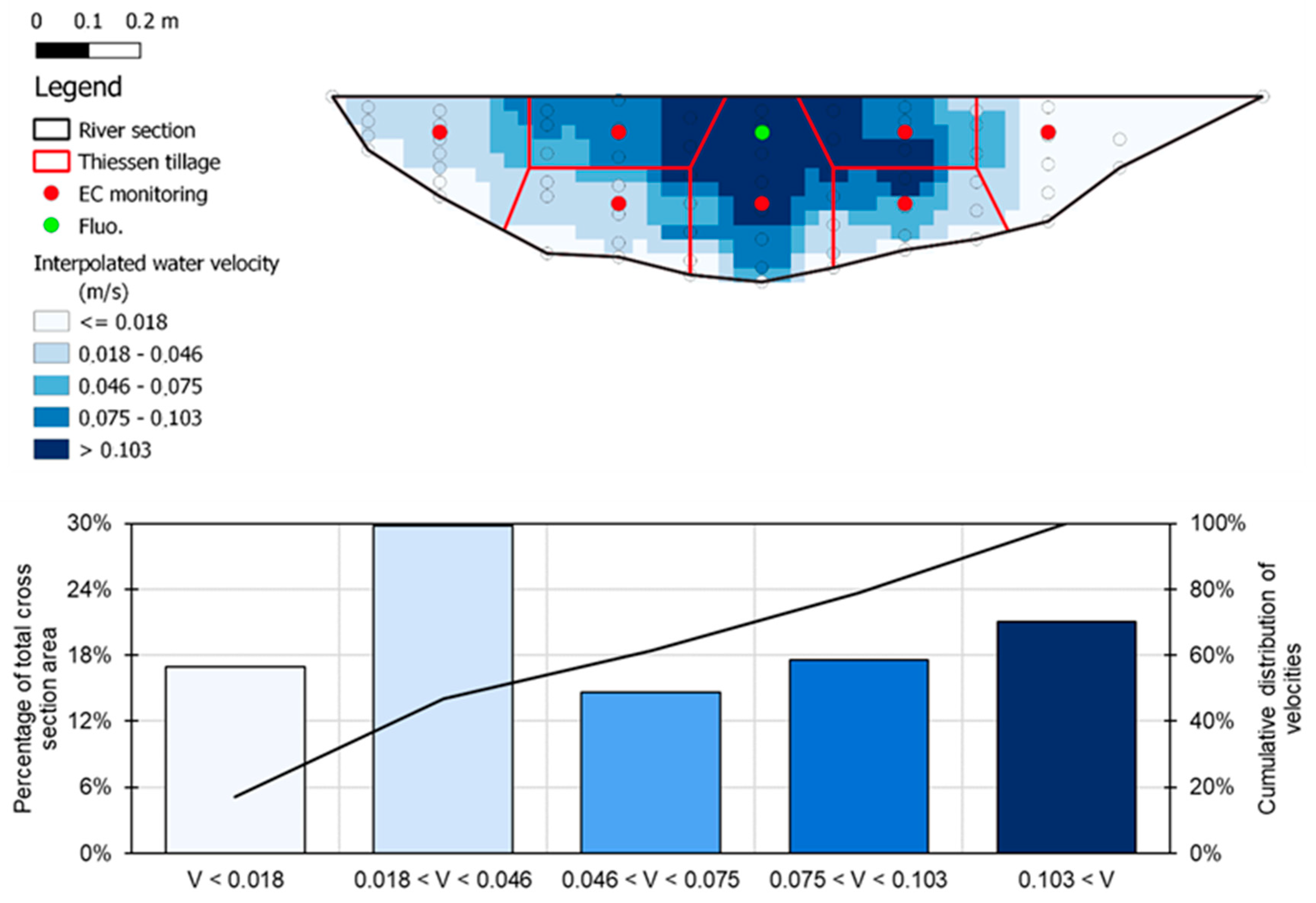
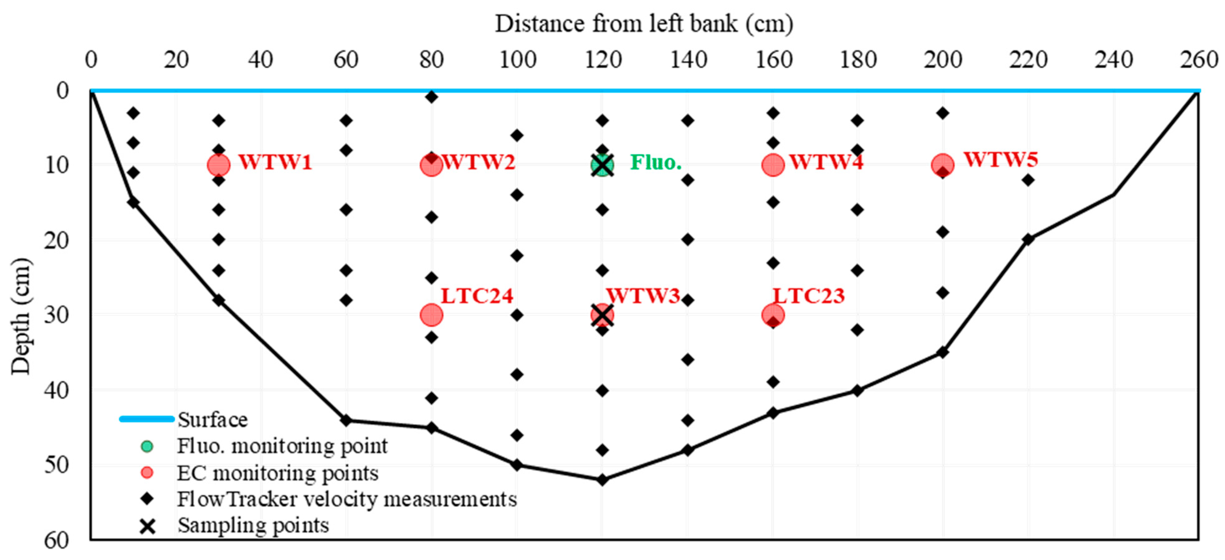
3.1. River Section Water Velocity Distribution

The survey performed using the FlowTracker allowed visualization of the water velocity distribution at the cross-section scale. The FlowTracker method yielded a discharge of 50.2 ± 3.6 L/s (

Table 1. Discharge values measured and associated uncertainties. Note that anion (Cl⁻, Br⁻) uncertainties were not available.

Measuring Point	Tracer Used	Discharge (L/s)	Uncertainties (L/s—%)	f (% of Total Flow)
FlowTracker	Velocity method	50.2	3.6–7.2	Not applicable
WTW1	Electrical conductivity	56.5	1.8–3.2	8.2
WTW2	Electrical conductivity	56.9	1.3–2.3	17.4
WTW3	Electrical conductivity	55.3	1.3–2.3	34.2
WTW4	Electrical conductivity	52.6	1.8–3.4	16.5
WTW5	Electrical conductivity	53.8	1.4–2.6	3.3
LTC 23	Electrical conductivity	49.8	1.1–2.2	11.4
LTC 24	Electrical conductivity	51.5	1.2–2.2	9.1
Composite restitution	Electrical conductivity	53.3	6.5–12.2	Not applicable
WTW3	2H	51.1	0.4–0.7	Not applicable
Fluo.	Tinopal	53.0	0.5–1.0	Not applicable
Fluo.	Uranine	60.6	0.8–1.4	Not applicable
Fluo.	37Cl	39.4	2.3–5.7	Not applicable
Fluo.	Cl−	41.3	Unknown	Not applicable
Fluo.	Br−	54.7	Unknown	Not applicable

). Zones of apparent stagnant water are identified near the banks (Figure 4), while most of the flow is in the centre of the stream at depths between 20 and 40 cm. Such discrepancies in the river velocities are expected to play a significant role in solute transport and on our tracing experiment. Their role on the interpretation of the tracer injection restitutions is discussed below.

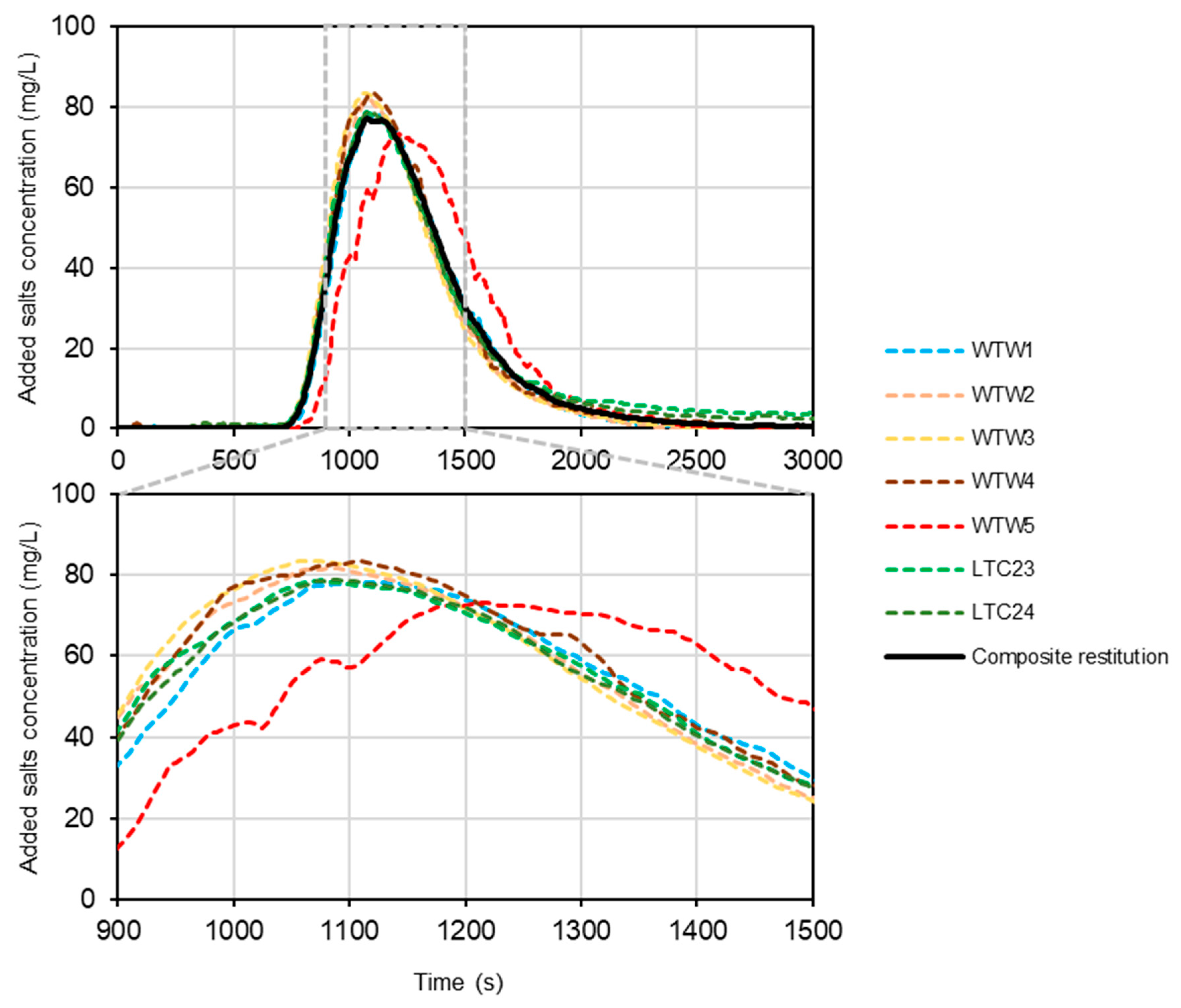
3.2. Using Salt Tracers to Build a Representative Restitution Curve for the Whole Section

A total of 7 restitution curves for electrical conductivity were obtained in the field. Restitution curves—expressed in mg/L of added salt tracers—are shown in Figure 5. The peak time is defined for each restitution curve as the time elapsed between the injection time and when the maximum concentration was measured. Tracer homogeneity across the river width was ensured at the injection point by laterally mixing the river water seconds after the injection. Except for WTW5, all restitution curves are very similar (Figure 5) in terms of peak time. This indicates that the transverse dispersion occurring along the reach is sufficient to ensure a good tracer homogeneity. The probe WTW5 was installed near the left bank in a zone of very low velocity with backwaters (Figure 4). Its peak height is lower than others and delayed with an increased peak width, which indicates tracer exchange between the main channel and transient storage zones [32,33].

Equations (4) and (5) were used to compute discharge values for each curve. In addition, the uncertainty propagation calculation was performed using the formula given in Equation (7). Discharge values are between 49.8 ± 1.1 and 56.9 ± 1.3 L/s. Most of them agree with the value obtained with the FlowTracker. However, the values obtained at measuring points WTW1, WTW2, and WTW3 are slightly above the value measured with the FlowTracker (Table 1). We suspect that there could be either a slight underestimation of the flow velocity measurements using the FlowTracker or an overestimation of the quantity of tracer. However, the latter is unlikely as it would shift all the obtained values and the quantities of tracer used were also thoroughly measured.

In all strictness, the second hypothesis of the use of Equation (4) (i.e., homogeneity of tracer concentration across the river section) is not entirely verified. We show below that Equation (4) can still be applied, with minimal effect on discharge calculations. To do so, we calculated a tracer output function averaged for the whole cross-section. This new restitution function (called “composite” in the following) includes the whole mass of tracer and is calculated as follows. Each restitution curve is supposed to be representative of the local tracer output. The river section was cut into seven sub-areas following Thiessen tillage (Figure 4), each of which were represented by one conductivity probe. The interpolated water velocity distribution presented in Figure 4 was then used to compute the discharge related to each sub-area. The latter is computed by multiplying the interpolated mean flow velocity by the surface of the sub-area. Typically, sub-areas near the banks have a lower discharge than the sub-areas located in the middle of the flow. The composite restitution function (see Figure 5) was then calculated as follows:

$${\mathrm{C}}_{\mathrm{composite}}\left(\mathrm{t}\right)=\sum _{\mathrm{i}=1}^7{\mathrm{C}}_{\mathrm{i}}\left(\mathrm{t}\right){\mathrm{f}}_{\mathrm{i}}$$

(12)

where i refers to the sub-area related to each probe (7 being the total number), C is the salt concentration [ML⁻³] and f_i is the fraction of total discharge passing by the sub-area i (adimensional). This cross-sectional flow-averaged function is very close to restitution functions obtained from the main flow channel since the weight of the dead zones is very limited. Indeed, the discharge and uncertainty propagation calculations yielded Q_composite = 53.3 ± 6.5 L/s, which is very close to discharges calculated over the cross-section. This strongly suggests that the “dilution” method is adapted to such small low-gradient streams with contrasted velocities. Furthermore, the calculation proposed in this work (Equation (12)) is adapted to any stream, especially if restitution functions are much different from the banks to the middle and requires (i) a precise survey of streamflow velocities across the whole section and (ii) the monitoring of tracers at various spots across the river section. The advantage of this function is that it verifies all the hypotheses of Equation (3) since it simulates the section-integrated homogenised tracer concentration dynamics. However, its main limitation is obviously the uncertainty propagation. While individual restitutions yield discharges values with uncertainties between 2.2% and 3.2%, the composite restitution gives uncertainties of 12.2%.

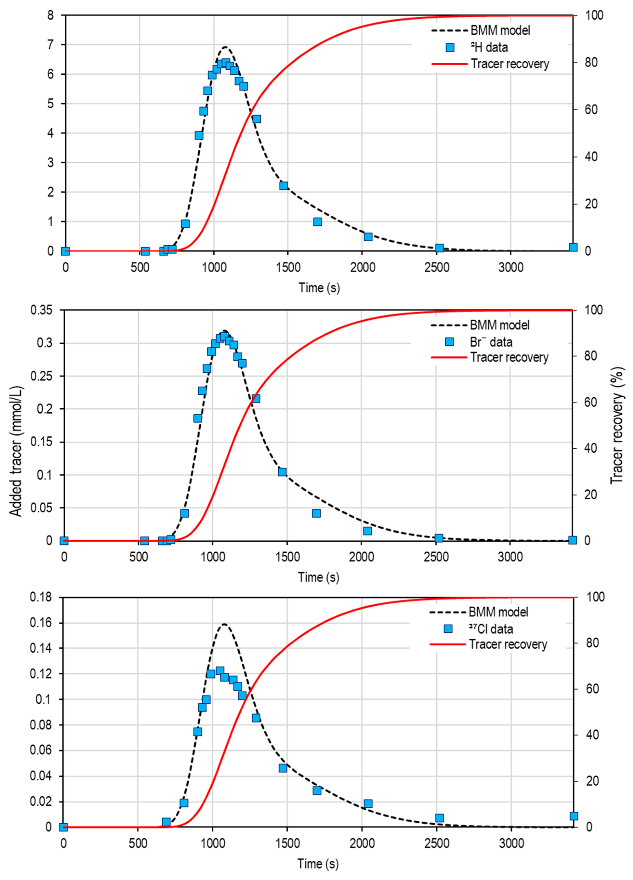
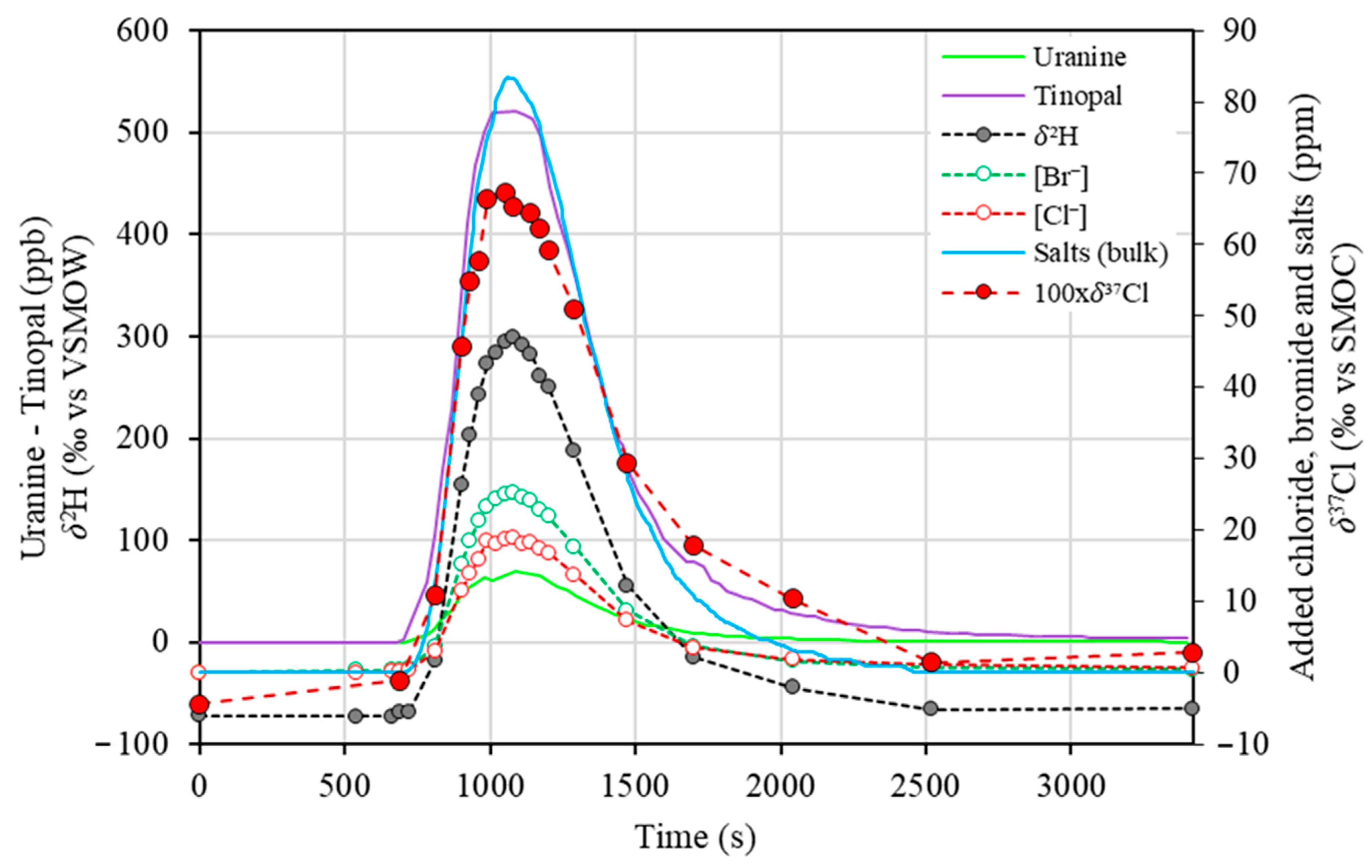
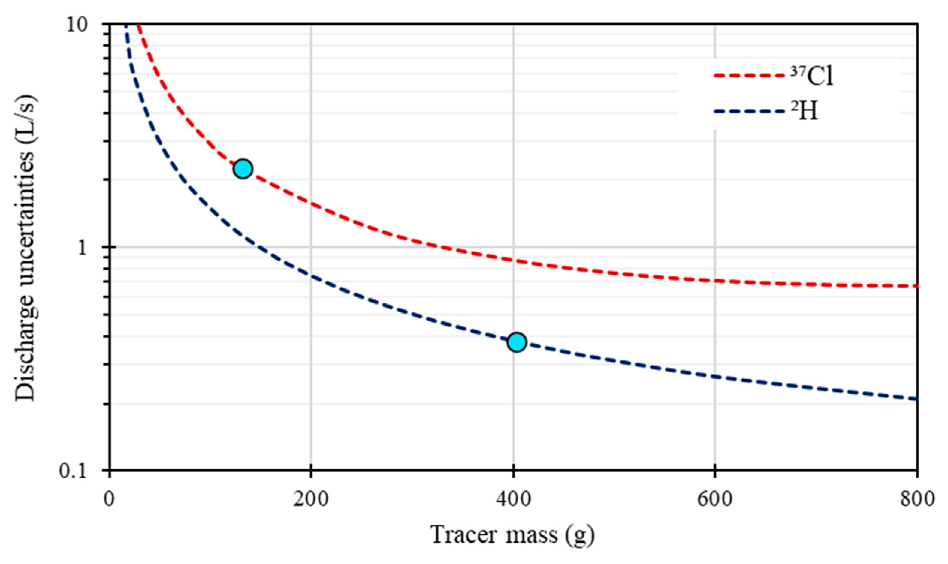
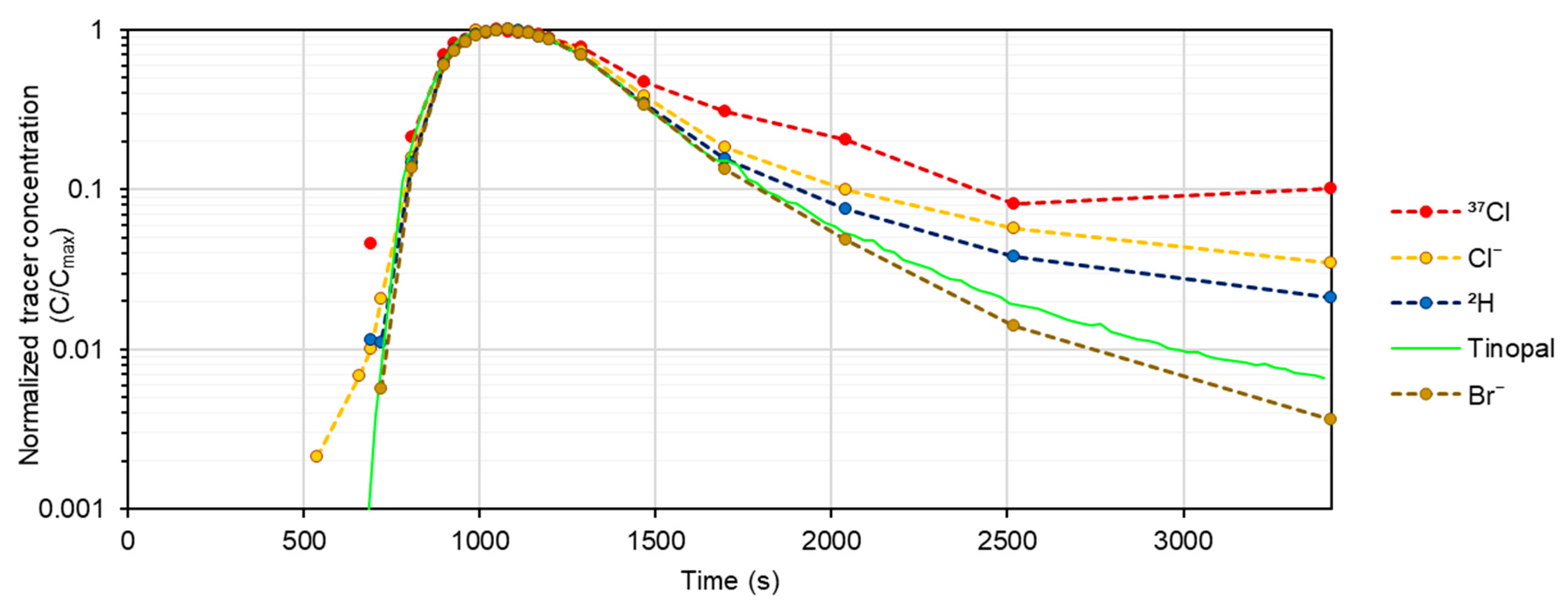
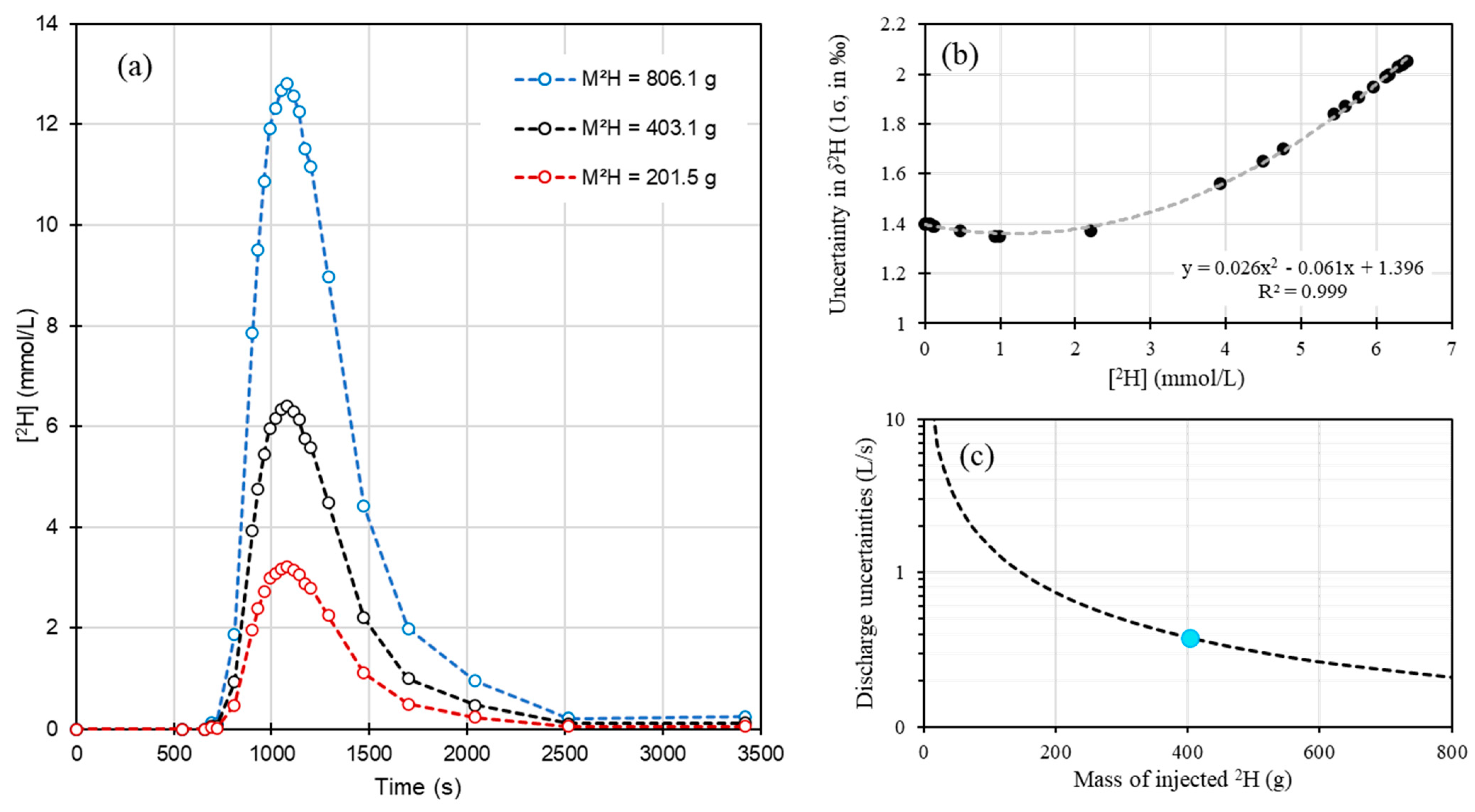
3.3. Isotopic Tracers as New Tracers for Discrete and Clean Discharge Measurements—Comparison with Other Tracers

Salt tracers are very useful for stream discharge measurements because they can easily be found, are inexpensive and are easy to monitor in the field thanks to electrical conductivity probes. However, their use can be very problematic in watersheds sheltering endangered ecosystems and species or used for surface drinking water production. In such contexts, it is worth to search for more adapted artificial tracers that can be injected in sufficiently low quantities that do not harm the environment and do not draw public attention like fluorescent dyes.

Stable isotopes tracers are now widely used in hydrology and hydrogeology as natural tracers [25,26,34,35]. Their use as artificial tracers is also reported in the literature, especially in the unsaturated zone and for tracing groundwater flows over short distances (see [25] and references therein). However, their potential for discrete, clean, and precise stream discharge measurements has not been addressed to date. In this work, heavy stable isotopes ²H (deuterated water, ²H₂O) and ³⁷Cl (isotopically enriched salt) were used as conservative tracers for quantitative interpretation of river discharge and comparison with other tracers.

The injected mass of each isotopic tracer was determined using the known mass of injected deuterated water and salt and their isotopic contents. Indeed, the deuterated water has a ²H abundancy of 99.90 ± 0.05%, and the ³⁷Cl-enriched salt has a δ³⁷Cl value of +2.18 ± 0.03‰ vs. SMOC, yielding totals of 403.09 ± 0.20 g of ²H and 131.17 g ± 0.09 g of ³⁷Cl. Stream discharge was computed using Equations (4) and (5), and uncertainty propagation was performed using Equation (7) (details for isotopes are also presented in Annex). Results are presented in Table 1 and the restitution curves of tracers can be found in Figure 6.

The highest discharge is obtained for uranine (60.6 ± 0.7 L/s). Only 2.42 g of uranine was injected, and a degradation of roughly 0.3 g could explain the shift obtained in discharge values. It is unlikely to have been considerably affected by photodegradation as the experiment time is less than 2 h, but it could be explained by an underestimation of the injected mass linked to the quality of the tracer and the fact that the calibration of the fluorometer was performed prior the field test using distilled water. Tinopal yielded a discharge value of 53.0 ± 0.5 L/s, which is in the same range as the FlowTracker measurement and electrical conductivity monitoring values. The discharge value obtained with deuterium is 51.1 ± 0.4 L/s, while ³⁷Cl data yielded a discharge of 39.4 ± 2.3 L/s. One must be aware that δ³⁷Cl measures uncertainties that are usually of the order of ±0.1‰, which is greater than the ±0.03‰ used in our calculations. These higher uncertainties would yield a total uncertainty of ±9.0 L/s (±22.9% of the discharge value). However, even though the discharge value obtained with ³⁷Cl is consistent with the discharge obtained using Cl⁻, it is very different from other tracers. The chloride and ³⁷Cl signals seem more concentrated relatively to other tracers’ signals.

Strictly speaking, for the same mass of a tracer, the use of ²H as an artificial tracer allows for a more precise discharge measure than the use of ³⁷Cl (Figure 7). The calculations used for Figure 7 are presented in the Appendix. However, even though deuterium analyses are widely affordable, the purchase of deuterated water is subject to governmental limitations, so one must be aware of potential difficulties in finding such a tracer in addition to the need for in-house produced enriched standards. On the other hand, while chloride is simple to find and cheap, ³⁷Cl-enriched salts are much harder to find. In addition, one must be aware that the background noise of ²H in rivers is commonly of the order of 140 to 156 ppm (for a δ²H ranging from −100‰ to 0‰ vs. VSMOW) and that the ³⁷Cl background noise of rivers with high chloride concentrations might be high because of the relatively high natural abundance of ³⁷Cl (³⁷R_SMOC = 0.324). In the quantities that were injected, deuterated water can be considered as the best tracer to measure stream discharge because it does not modify or alter the qualitative and ecological state of the stream while being a robust and extremely precise tracer.

3.4. Transient Storage Zone Exchanges Inferred from Multi-Tracer Data

When a tracer is injected into the stream, advective-dispersive transport will result in solute tracer homogenization over the river width due to transverse dispersion and a classical Gaussian form of the restitution function due to longitudinal dispersion. However, the tracer will also exchange with transient storage zones, such as dead zones near the banks and/or the hyporheic zone at the bottom of the stream, and will be slowly released to the main flow channel [17,18,20]. Transport in the hyporheic zone is known for being mainly advective [15]. Since tracer residence times in the transient storage zones are typically several orders of magnitude higher than those of the tracer in the stream alone, information on hyporheic exchanges can be found on the tailing part of the breakthrough curves.

Here, we took advantage of having multiple tracer restitutions to study the interactions between the stream and the hyporheic zone in more detail. Normalized breakthrough curves (C/C_max) of tinopal, ²H, ³⁷Cl, Br⁻, and Cl⁻ show different behaviours during the tailing part of the experiment (Figure 8). If we define persistence as the affinity of the tracer to stay in the stream for long times, bromide is the least persistent tracer, while chloride (and especially ³⁷Cl) is the most persistent. ²H lies in between, and being part of the water molecule, is the ideal tracer of the latter. It seems that the surface solute transport is affected by one (or more) hydrological unit(s) that acts as a filter, filtering the entrance of the tracer and thus controlling the residence time of tracer within it. Such a hydrological unit could be a surface transient storage zone and/or hyporheic zone.

Since the tracers used in this study have different chemical and physical properties, we can expect them to behave differently regarding hyporheic and surface dead zone exchanges. Exchanges between the stream and the subsurface (e.g., the hyporheic zone) are controlled by the streambed permeability and porosity [15] but might also be controlled by the effective accessible pore size of tracers. Bromide restitution shows a lower tailing effect, meaning that it is less affected by such exchanges than ²H and ³⁷Cl. The breakthrough curves of the latter two indicates that the release of chloride is slower than that of deuterium. This makes sense, as chloride transport in a porous media might be slowed due to its size compared to ²H. Tinopal was expected to fall below the Br⁻ curve since it is the largest molecule used (chemical formula: C₄₀H₄₀N₁₂O₈S₂). Because of its high susceptibility to be absorbed to suspended particles, such as clays and organic matter, and its low effective solubility [36,37], tinopal is often not considered a totally conservative tracer. This results in a prolonged tailing effect, that might explain why it is more “persistent” than bromide.

Bromide, ³⁷Cl, and ²H restitution curves were fitted to the binary mixing model described in Equations (9)–(11) (Figure 9). The f₁ parameter that represents the fraction of the fast component as well as its velocity, v₁, were set as the same for all tracers because this part of the flow is controlled by advective transport and should not vary from one tracer to the other. However, parameters for the slow component (dispersion and velocity) were set to vary to model the differences in tailing seen in Figure 8 and account for the different behaviours of tracers. The set of parameters that provided the best fit is given in the

Table 2. Best-fit set of parameters for the modelling of solute transport affected by diffusive transfer in the hyporheic zone.

		g1 Parameters		g2 Parameters
Tracer	f1	D1 (m2/s)	v1 (m/s)	D2 (m2/s)	v2 (m/s)	χ2 (mol/L)
2H		0.10	0.097	0.20	0.068	9.5 × 10−4
37Cl	0.58	0.13	0.097	0.39	0.053	7.5 × 10−5
Br−		0.10	0.097	0.26	0.070	6.2 × 10−5

. The transient zone storage fraction, f₂ (f₂ = 1 − f₁), is 0.42. This means that it exerts a very strong influence in the transport characteristics of the dissolved solutes. It is thought to be the fraction of the flow that is affected by both surface transient storage and transport within the hyporheic zone. Bromide and deuterium breakthrough curves are well modelled, especially at longer times. However, ³⁷Cl is affected by another phenomenon. Indeed, we saw earlier that the discharge measured using both chloride and its heavy isotope was somewhat less than that noted with other tracers. In addition, the model predicts a higher concentration than what was measured in the field. It is still unclear why chloride behaves in such a way.

4. Conclusions

Solute transport in a small low-gradient stream was studied under baseflow conditions. The stream is characterized by contrasting channel characteristics with a succession of small riffles and pools. The cross-sectional dynamics of salt tracers (monitored using the electrical conductivity signal) revealed a very good homogenization of the tracers, except in a large dead zone near one of the banks. The computation of a composite tracer restitution, integrating the cross-sectional dynamics, showed that the “dilution” method is still applicable in such small, low-gradient, heterogeneous streams. Stable isotopes ²H and ³⁷Cl are reliable tracers for discharge measurements in small streams. In addition, deuterium revealed to be an excellent tracer for such an experiment since it can be released in the environment in very small quantities without any environmental effect and still yielded more precise results than traditional tracers.

This multi-tracer (Br⁻, Cl⁻, ²H, ³⁷Cl, uranine, tinopal and the electrical conductivity signal) approach also allows depiction of the river solute transport in detail, especially the identification of the behaviours of solutes over the longer residence times. The tailing part differences of the restitution curve of the tracers Br⁻, Cl⁻, ²H, ³⁷Cl, and tinopal are attributed to differences in the tracers’ behaviours regarding transient storage zones. However, chloride shows an unexpected, prolonged tailing effect. It is unclear whether chloride was affected by another chemical process as the signal seems “diluted” relative to the other tracers. Further investigations should be performed using such a multi-tracer approach for longer experiments, including the multi-injection and monitoring of inert and reactive gases in the stream (e.g., He, N₂, C₃H₈), to explore their potential for stream discharge measurements and transient-zone storage interactions.

References

1. Herschy, R.W. Streamflow Measuremen; Francis, T., Ed.; CRC Press: Boca Raton, FL, USA, 2008; 534p. [Google Scholar]
2. WMO. Guide to Hydrological Practice Volume I—From Measurement to Hydrological Information; WMO: Geneva, Switzerland, 2008. [Google Scholar]
3. Jensen, C.R.; Genereux, D.P.; Gilmore, T.E.; Solomon, D.K.; Mittelstet, A.R.; Humphrey, C.E.; MacNamara, M.R.; Zeyrek, C.; Zlotnik, V.A. Estimating groundwater mean transit time from SF6 in stream water: Field example and planning metrics for a reach mass-balance approach. Hydrogeol. J. 2022, 30, 479–494. [Google Scholar] [CrossRef]
4. Cook, P.G.; Lamontagne, S.; Berhane, D.; Clark, J.F. Quantifying groundwater discharge to Cockburn River, southeastern Australia, using dissolved gas tracers 222Rn and SF6. Water Resour. Res. 2006, 42, 12. [Google Scholar] [CrossRef]
5. Le Coz, J.; Camenen, B.; Dramais, G.; Ribot-Bruno, J.; Ferry, M.; Rosique, J.L. Guide Technique Pour le Contrôle des Débits Réglementaires; ONEMA, Cemagref: Vincennes, France, 2011; 132p. [Google Scholar]
6. WMO. Manual on Stream Gauging Volume I—Fieldwork; WMO: Geneva, Switzerland, 2010. [Google Scholar]
7. Pelletier, P.M. Uncertainties in the single determination of river discharge: A literature review. Can. J. Civ. Eng. 1988, 15, 834–850. [Google Scholar] [CrossRef]
8. Tazioli, A. Experimental methods for river discharge measurements: Comparison among tracers and current meter. Hydrol. Sci. J. 2011, 56, 1314–1324. [Google Scholar] [CrossRef]
9. Hudson, R.; Fraser, J. The Mass Balance (or Dry Injection) Method. Watershed Manag. Bull. 2005, 9, 6–12. [Google Scholar]
10. Winter, T.C.; Harvey, J.W.; Franke, O.L.; Alley, W.M. Ground Water and Surface Water, a Single Resource; Circular 1139; USGS: Reston, VA, USA, 1998; 87p.
11. Sophocleous, M. Interactions between groundwater and surface water: The state of the science. Hydrogeol. J. 2002, 10, 52–67. [Google Scholar] [CrossRef]
12. Gooseff, M.N. Defining Hyporheic Zones—Advancing Our Conceptual and Operational Definitions of Where Stream Water and Groundwater Meet. Geogr. Compass 2010, 4, 945–955. [Google Scholar] [CrossRef]
13. Engelhardt, I.; Piepenbrink, M.; Trauth, N.; Stadler, S.; Kludt, C.; Schulz, M.; Schüth, C.; Ternes, T. Comparison of tracer methods to quantify hydrodynamic exchange within the hyporheic zone. J. Hydrol. 2011, 400, 255–266. [Google Scholar] [CrossRef]
14. Beck, H.E.; van Dijk, A.I.J.M.; Miralles, D.G.; de Jeu, R.A.M.; Bruijnzeel, L.A.; McVicar, T.R.; Schellekens, J. Global patterns in base flow index and recession based on streamflow observations from 3394 catchments. Water Resour. Res. 2013, 49, 7843–7863. [Google Scholar] [CrossRef]
15. Boano, F.; Harvey, J.W.; Marion, A.; Packman, A.I.; Revelli, R.; Ridolfi, L.; Wörman, A. Hyporheic flow and transport processes: Mechanisms, models, and biogeochemical implications. Rev. Geophys. 2014, 52, 603–679. [Google Scholar] [CrossRef]
16. Battin, T.J.; Kaplan, L.A.; Findlay, S.; Hopkinson, C.S.; Marti, E.; Packman, A.I.; Newbold, J.D.; Sabater, F. Biophysical controls on organic carbon fluxes in fluvial networks. Nat. Geosci. 2008, 1, 95–101. [Google Scholar] [CrossRef]
17. Runkel, R.L. One-Dimensional Transport with Inflow and Storage (OTIS): A Solute Transport Model for Streams and Rivers; USGS: Denver, CO, USA, 1998.
18. van Genuchten, M.T.; Leij, F.J.; Skaggs, T.H.; Toride, N.; Bradford, S.A.; Pontedeiro, E.M. Exact Analytical Solutions for Contaminant Transport in Rivers. 2. Transient storage and decay chain solutions. J. Hydrol. Hydromech. 2013, 61, 250–259. [Google Scholar] [CrossRef]
19. van Genuchten, M.T.; Leij, F.J.; Skaggs, T.H.; Toride, N.; Bradford, S.A.; Pontedeiro, E.M. Exact analytical solutions for contaminant transport in rivers. 1. The equilibrium advection-dispersion equation. J. Hydrol. Hydromech. 2013, 61, 146–160. [Google Scholar] [CrossRef]
20. De Smedt, F. Analytical solution and analysis of solute transport in rivers affected by diffusive transfer in the hyporheic zone. J. Hydrol. 2007, 339, 29–38. [Google Scholar] [CrossRef]
21. Søndergaard, M.; Jeppesen, E. Anthropogenic impacts on lake and stream ecosystems, and approaches to restoration. J. Appl. Ecol. 2007, 44, 1089–1094. [Google Scholar] [CrossRef]
22. Verhoeven, J.T.; Arheimer, B.; Yin, C.; Hefting, M. Regional and global concerns over wetlands and water quality. Trends Ecol. Evol. 2006, 21, 96–103. [Google Scholar] [CrossRef]
23. Barlow, P.M.; Leake, S.A. Streamflow Depletion by Wells—Understanding and Managing the Effects of Groundwater Pumping on Streamflow; USGS: Reston, VA, USA, 2012; 95p.
24. Wood, P.J.; Dykes, A.P. The use of salt dilution gauging techniques: Ecological considerations and insights. Water Res. 2002, 36, 3054–3062. [Google Scholar] [CrossRef]
25. Leibundgut, C.; Maloszewski, P.; Külls, C. Tracers in Hydrology; Wiley-Blackwell: Hoboken, NJ, USA, 2009. [Google Scholar]
26. Clark, I.D.; Fritz, P. Environmental Isotopes in Hydrogeology; CRC Press: Boca Raton, FL, USA, 1997. [Google Scholar]
27. SIGEOM. Available online: https://sigeom.mines.gouv.qc.ca/ (accessed on 23 October 2023).
28. Kaufman, R.S.; Long, A.; Bentley, H.; Davis, S. Natural chlorine isotope variations. Nature 1984, 209, 338–340. [Google Scholar] [CrossRef]
29. Eggenkamp, H.G.M. The Geochemistry of Stable Chlorine and Bromine Isotopes; Utrecht University: Utrecht, The Netherlands, 1994. [Google Scholar]
30. Godon, A.; Jendrzejewski, N.; Eggenkamp, H.G.; Banks, D.A.; Ader, M.; Coleman, M.L.; Pineau, F. A cross-calibration of chlorine isotopic measurements and suitability of seawater as the international reference material. Chem. Geol. 2004, 207, 1–12. [Google Scholar] [CrossRef]
31. Jurgens, B.C.; Böhlke, J.K.; Eberts, S.M. TracerLPM (Version 1): An Excel Workbook for Interpreting Groundwater Age Distributions from Environmental Tracer Data; USGS: Reston, VA, USA, 2012; 72p.
32. Runkel, R.L.; Chapra, S.C. An efficient numerical solution of the transient storage equations for solute transport in small streams. Water Resour. Res. 1993, 29, 211–215. [Google Scholar] [CrossRef]
33. Briggs, M.A.; Gooseff, M.N.; Arp, C.D.; Baker, M.A. A method for estimating surface transient storage parameters for streams with concurrent hyporheic storage. Water Resour. Res. 2009, 45. [Google Scholar] [CrossRef]
34. Cook, P.G.; Herczeg, A.L. Environmental Tracers in Subsurface Hydrology; Springer Science: Berlin/Heidelberg, Germany, 2000. [Google Scholar]
35. Clark, I.D. Groundwater Geochemistry and Isotopes; CRC Press: Boca Raton, FL, USA, 2015. [Google Scholar]
36. Licha, T.; Niedbala, A.; Bozau, E.; Geyer, T. An assessment of selected properties of the fluorescent tracer, Tinopal CBS-X related to conservative behavior, and suggested improvements. J. Hydrol. 2013, 484, 38–44. [Google Scholar] [CrossRef]
37. Schiperski, F.; Oertwich, M.; Scheytt, T.; Licha, T. Solubility of TINOPAL CBS-X fluorescent dye at different EDTA concentrations and pH values: Implications regarding its applicability in field tracer tests. J. Hydrol. 2019, 578, 124025. [Google Scholar] [CrossRef]
Figure 1. Map of Canada (on the left) and of the Ruisseau Rousse watershed (on the right). The red dots in both maps symbolise where the field work occurred.
Hydrology 11 00001 g001
Figure 2. (On the left): picture of the stream at the injection site (under a small culvert). We ensured tracer homogeneity by manually fanning the water under the culvert. (On the right): picture of the restitution site with the equipment used to monitor solute concentration.
Hydrology 11 00001 g002
Figure 3. River working section (looking upstream) with equipment location.
Hydrology 11 00001 g003
Figure 4. Distribution of interpolated river water velocity (n = 342). A value of zero was forced at the streambed and above the water surface for the spatial interpolation. Velocities are expressed in m.s−1.
Hydrology 11 00001 g004
Figure 5. Upper graph: the seven salts concentration restitution functions and the composite restitution function. Lower graph: zoom-in around the peak time showing slight differences in peak heights. Background initial concentrations were removed, which explains the zero concentration at the beginning of the experiment.
Hydrology 11 00001 g005
Figure 6. 2H, 37Cl, Cl, Br and fluorescent tracers (uranine, tinopal) restitutions obtained at the centre of the stream.
Hydrology 11 00001 g006
Figure 7. Discharge measure uncertainty as a function of mass of injected tracer (2H, 37Cl) for the studied river (the blue dots represent this experiment). It is important to note that the x-axis refers to the actual isotopic tracer’s mass alone and not 37Cl-enriched salt or deuterated water. Details on these calculations can be found in Appendix A.
Hydrology 11 00001 g007
Figure 8. Normalized tracer restitution showing different tracer behaviours at times >1500 s.
Hydrology 11 00001 g008
Figure 9. Tracers’ concentrations modelled using a binary mixing 1D dispersion model.
Hydrology 11 00001 g009