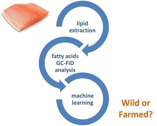
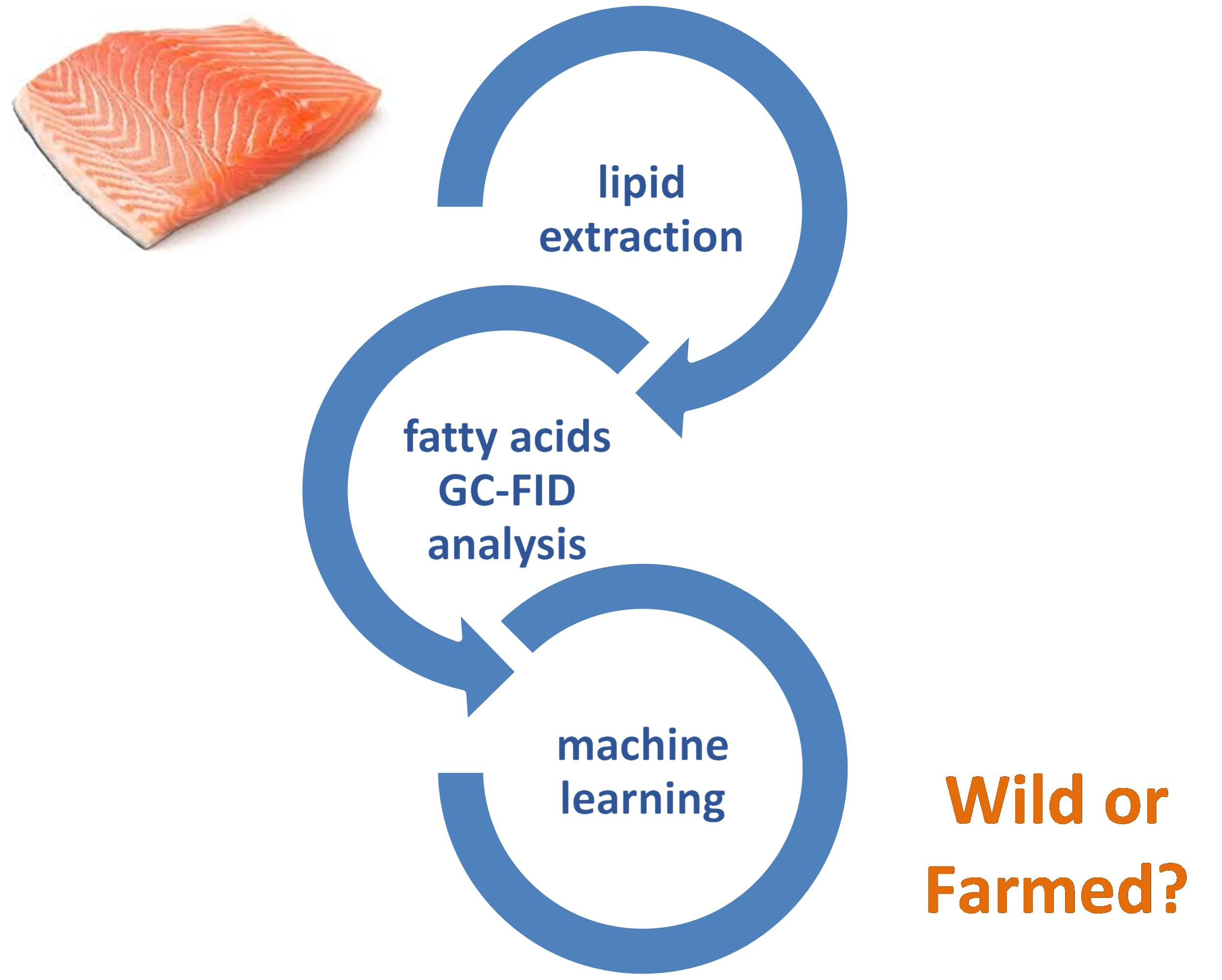
Machine Learning Approaches Applied to GC-FID Fatty Acid Profiles to Discriminate Wild from Farmed Salmon

 ,
,  ,
,  and
and 
Abstract
:
1. Introduction
2. Materials and Methods
2.1. Samples
2.2. Lipid Extraction
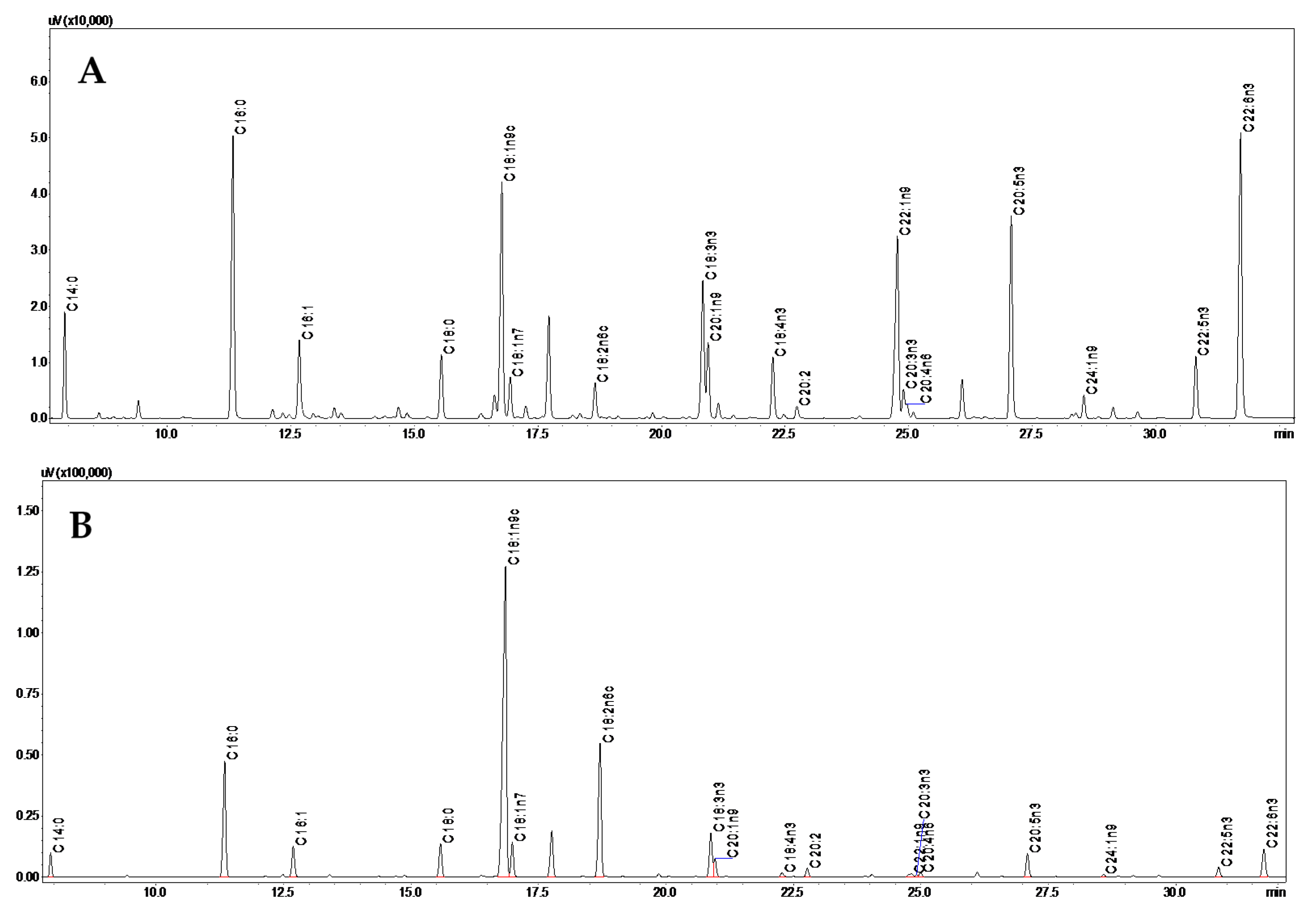
2.3. Fatty Acids Analysis by GC-FID
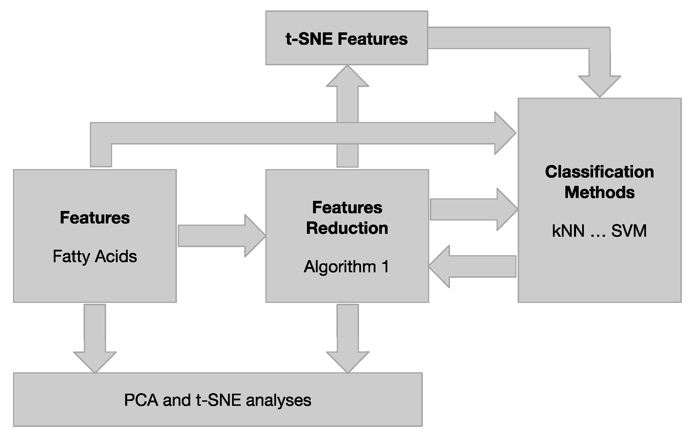
2.4. Chemometric Analysis
2.4.1. Dataset
2.4.2. Statistical Analysis by One-Way ANOVA
2.4.3. Data Modelling Tools
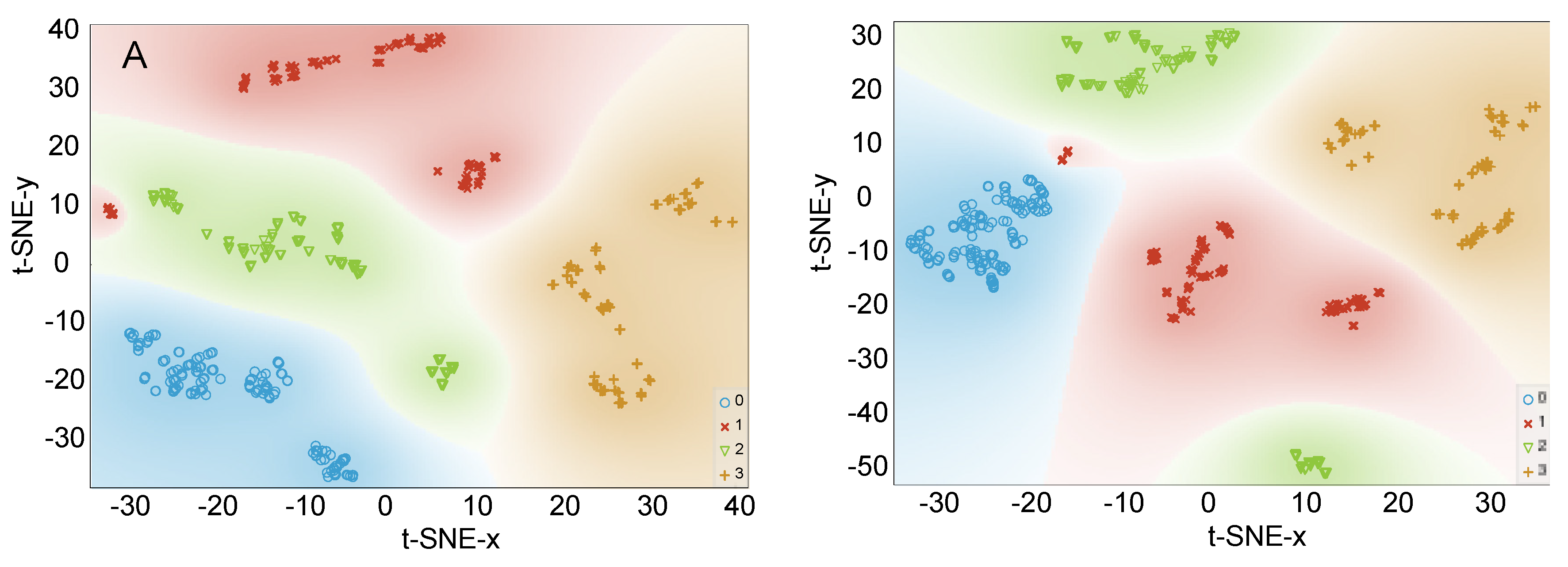
Data Visualization by PCA and t-SNE
Machine Learning Classifiers
- kNN is a method that can be used for data classification. A sample is classified by the rating vote of its neighbors present in the dataset; the result is attributed to the most common class among the k closest neighbors. If k = 1, the object is simply assigned to the class of the only nearest neighbour [26].
- Decision tree is one of the predictive modeling approaches used in machine learning. It uses a tree schema as a predictive model to move from the analysis of a sample to conclude the class that corresponds to the sample. The decision trees are built inductively from a dataset that is analyzed by measures, such as the information entropy. During the process, the dataset is divided, successively, in order to reduce the uncertainty in the classification. That division is represented by each feature (tree node) [27].
- Support-vector machines (SVM) are models of supervised learning. Given a set of training examples, each is marked as belonging to one or the other of two categories. The resulting model, after training, is a representation of the examples as points in space, mapped so that the widest possible spatial margin separates the examples of the two categories. The new examples are expected to belong to a category based on the margin side where they are located. That side is formed from the center of the separating margin. This process leads to the fact that SVM can generalize as best as possible, avoiding overfitting. In addition to performing linear mapping, SVM can efficiently perform non-linear mapping using what is called a kernel trick, implicitly mapping their inputs into high-dimensional spaces, allowing separations to happen in the high dimensional space [28].
- Random forests are a learning method that can be used for classification. They are built based on decision trees, but in this case, there is a participation of several trees that are trained with segments of the dataset and with segments of the feature set randomly selected [29]. This stochastic factor improves the generalization of the model and reduces the overfitting.
- Artificial neural networks (ANN) is a model based on a collection of connected units or nodes called “artificial neurons”, which mimic neurons in a biological brain. Each connection can transmit signals from one artificial neuron to another; the magnitude of the signal is modulated by a parameter adjusted during the learning phase. Each neuron behaves like a separating hyperplane in the classification space. The association of neurons, by layers, allows obtaining conjugations of complex hyperplanes that lead to non-linear classification models. The adjustment of the parameters is made by algorithms that use the gradient descent of the error. The error is defined by the difference between the value emitted by the neural network and the desired value [30].
- Naïve Bayes, in machine learning, are probabilistic classifiers, based on the application of Bayes’ theorem with evidence on the assumptions of independence between features [31]. Naïve Bayes classifiers are easy to implement using Gaussian curves and the inverse Bayes formula.
- AdaBoost (short for adaptive boosting) is based on the idea that a set of weak classifiers can result in a strong classifier. Weak classifiers are combined linearly, but modulated by coefficients that are obtained during the training. The choice of weak classifiers is made focusing on the examples that are classified with more difficulty. In this iterative process, the weak classifiers have coefficients that correspond to the classifier error on the dataset. The weak classifiers that make the least mistakes have their coefficients increased. The strong classifier aggregates all those weak classifiers according to their importance coefficients [32].
Reduction in Features
| Algorithm 1 Searching the optimal number of features |
Given a set of features F of n elements with gain ratio values F0, F1, F2, …, Fn−1 sorted such that F0 > F1 > F2 … > Fn−1, and the accuracym being the correctness classifying the dataset using the first m features. The following algorithm is based on the binary search to find the index m in F that corresponds to the minimum index to classify the dataset properly.
|
3. Results and Discussion
3.1. Fatty Acids Composition
3.2. Chemometric Analysis of the Generated Data
3.2.1. Features Selection
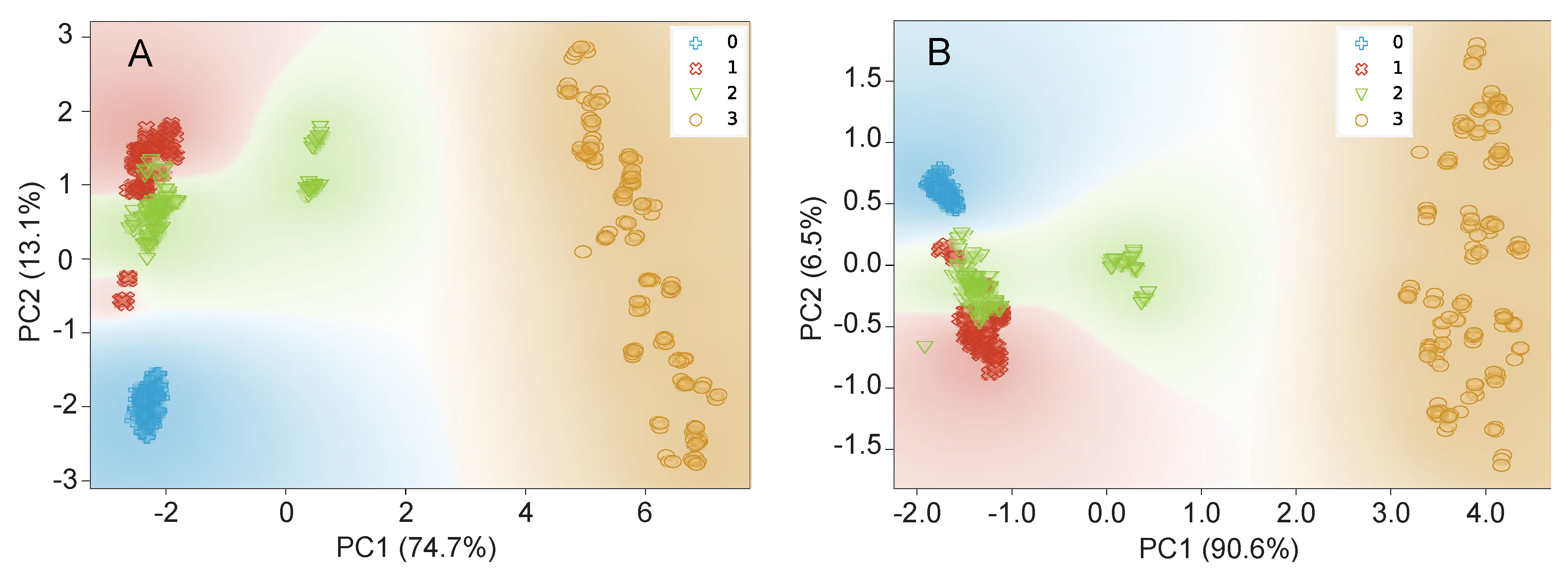
3.2.2. Data Visualization by PCA and t-SNE
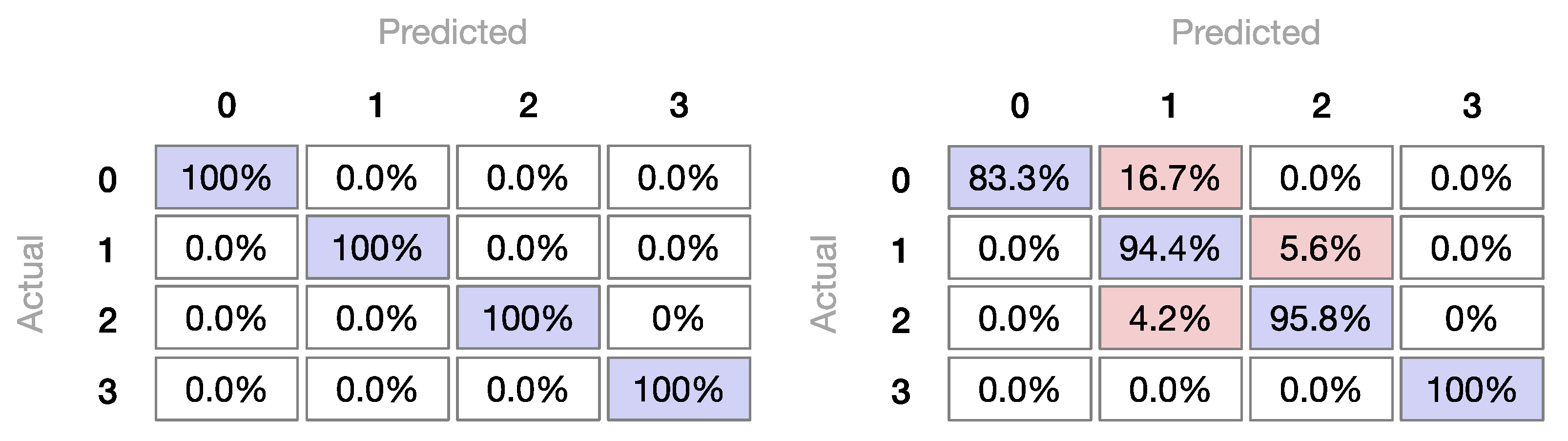
3.2.3. Machine Learning Classifiers
4. Conclusions
Author Contributions
Funding
Acknowledgments
Conflicts of Interest
References
- Larsen, R.; Eilertsen, K.E.; Elvevoll, E.O. Health benefits of marine foods and ingredients. Biotechnol. Adv. 2011, 29, 508–518. [Google Scholar] [CrossRef]
- Swanson, D.; Block, R.; Mousa, S.A. Omega-3 Fatty Acids EPA and DHA: Health Benefits Throughout Life. Adv. Nutr. 2012, 3, 1–7. [Google Scholar] [CrossRef]
- Shahidi, F.; Ambigaipalan, P. Omega-3 polyunsaturated fatty acids and their health benefits. Annu. Rev. Food Sci. Technol. 2018, 9, 345–381. [Google Scholar] [CrossRef]
- FAO Food and Agriculture Organization (FAO). GLOBEFISH Highlights Issue 1/2020, with Jan.–Sep. 2019 Statistics—A Quarterly Update on World Seafood Markets. 2020. Available online: http://www.fao.org/3/ca7968en/CA7968EN.pdf (accessed on 26 August 2020).
- FAO Food and Agriculture Organization (FAO). Salmon Commodity Statistics Update. 2016. Available online: http://www.fao.org/3/a-bq971e.pdf (accessed on 26 August 2020).
- Blanchet, C.; Lucas, M.; Julien, P.; Morin, R.; Gingras, S.; Dewailly, E. Fatty acid composition of wild and farmed Atlantic salmon (Salmo salar) and rainbow trout (Oncorhynchus mykiss). Lipids 2005, 40, 529–531. [Google Scholar] [CrossRef]
- Lundebye, A.K.; Lock, E.J.; Rasinger, J.D.; Nøstbakken, O.J.; Hannisdal, R.; Karlsbakk, E.; Wennevik, V.; Madhun, A.S.; Madsen, L.; Graff, I.E.; et al. Lower levels of persistent organic pollutants, metals and the marine omega 3-fatty acid DHA in farmed compared to wild Atlantic salmon (Salmo salar). Environ. Res. 2017, 155, 49–59. [Google Scholar] [CrossRef]
- Fiorino, G.M.; Ilario, L.; De Angelis, E.; Arlorio, M.; Logrieco, A.F.; Monaci, L. Assessing fish authenticity by direct analysis in real time-high resolution mass spectrometry and multivariate analysis: Discrimination between wildtype and farmed salmon. Food Res. Int. 2019, 116, 1258–1265. [Google Scholar] [CrossRef]
- Kappel, K.; Schröder, U. Substitution of high-priced fish with low-priced species: Adulteration of common sole in German restaurants. Food Control 2016, 59, 478–486. [Google Scholar] [CrossRef]
- Cline, E. Marketplace substitution of Atlantic salmon for Pacific salmon in Washington State detected by DNA barcoding. Food Res. Int. 2012, 45, 388–393. [Google Scholar] [CrossRef]
- Thomas, F.; Jamin, E.; Wietzerbin, K.; Guérin, R.; Lees, M.; Morvan, E.; Billault, I.; Derrien, S.; Rojas, J.M.M.; Serra, F.; et al. Determination of origin of Atlantic salmon (Salmo salar): The use of multiprobe and multielement isotopic analyses in combination with fatty acid composition to assess wild or farmed origin. J. Agric. Food Chem. 2008, 56, 989–997. [Google Scholar] [CrossRef]
- Fernandes, T.J.R.; Amaral, J.S.; Mafra, I. DNA barcode markers applied to seafood authentication: An updated review. Crit. Rev. Food Sci. Nutr. 2020, in press. [Google Scholar] [CrossRef]
- Aursand, M.; Standal, I.B.; Prael, A.; McEvoy, L.; Irvine, J.; Axelson, D.E. C-13 NMR pattern recognition techniques for the classification of Atlantic salmon (Salmo salar L.) according to their wild, farmed, and geographical origin. J. Agric. Food Chem. 2009, 57, 3444–3451. [Google Scholar] [CrossRef]
- Masoum, S.; Malabat, C.; Jalali-Heravi, M.; Guillou, C.; Rezzi, S.; Rutledge, D.N. Application of support vector machines to 1 H NMR data of fish oils: Methodology for the confirmation of wild and farmed salmon and their origins. Anal. Bioanal. Chem. 2007, 387, 1499–1510. [Google Scholar] [CrossRef]
- Molkentin, J.; Meisel, H.; Lehmann, I.; Rehbein, H. Identification of organically farmed Atlantic salmon by analysis of stable isotopes and fatty acids. Eur. Food Res. Technol. 2007, 224, 535–543. [Google Scholar] [CrossRef]
- Dempson, J.B.; Power, M. Use of stable isotopes to distinguish farmed from wild Atlantic salmon, Salmo salar. Ecol. Freshw. Fish 2004, 13, 176–184. [Google Scholar] [CrossRef]
- Megdal, P.A.; Craft, N.A.; Handelman, G.J. A simplified method to distinguish farmed (Salmo salar) from wild salmon: Fatty acid ratios versus astaxanthin chiral isomers. Lipids 2009, 44, 569–576. [Google Scholar] [CrossRef] [Green Version]
- Axelson, D.E.; Standal, I.B.; Martinez, I.; Aursand, M. Classification of wild and farmed salmon using bayesian belief networks and gas chromatography-derived fatty acid distributions. J. Agric. Food Chem. 2009, 57, 7634–7639. [Google Scholar] [CrossRef]
- Martinez, I.; Standal, I.B.; Axelson, D.E.; Finstad, B.; Aursand, M. Identification of the farm origin of salmon by fatty acid and HR C-13 NMR profiling. Food Chem. 2009, 116, 766–773. [Google Scholar] [CrossRef]
- Molkentin, J.; Lehmann, I.; Ostermeyer, U.; Rehbein, H. Traceability of organic fish e Authenticating the production origin of salmonids by chemical and isotopic analyses. Food Control 2015, 53, 55–66. [Google Scholar] [CrossRef]
- Aursand, M.; Mabon, F.; Martin, G.J. Characterization of farmed and wild salmon (Salmo salar) by a combined use of compositional and isotopic analyses. JAOCS 2000, 77, 659–666. [Google Scholar] [CrossRef]
- Bligh, E.G.; Dyer, W.J. A rapid method of total lipid extraction and purification. Can. J. Biochem. Physiol. 1959, 37, 911–917. [Google Scholar] [CrossRef] [Green Version]
- Amaral, J.S.; Casal, S.; Pereira, J.A.; Seavra, R.M.; Oliveira, M.B.P.P. Determination of sterol and fatty acid compositions, oxidative stability, and nutritional value of six walnut (Juglans regia L.) cultivars grown in Portugal. J. Agric. Food Chem. 2003, 51, 7698–7702. [Google Scholar] [CrossRef] [Green Version]
- Jolliffe, I.T. Principal Component Analysis, 2nd ed.; Springer Inc.: New York, NY, USA, 2002. [Google Scholar]
- Van der Maaten, L.J.P.; Hinton, G.E. Visualizing Data Using t-SNE. J. Mach. Learn. Res. 2008, 9, 2579–2605. [Google Scholar]
- Altman, N.S. An introduction to kernel and nearest-neighbor nonparametric regression. Am. Stat. 1992, 46, 175–185. [Google Scholar]
- Quinlan, J.R. Simplifying decision trees. Int. J. Man. Mach. Stud. 1987, 27, 221–234. [Google Scholar] [CrossRef] [Green Version]
- Cortes, C.; Vapnik, V.N. Support-vector networks. Mach. Learn. 1995, 20, 273–297. [Google Scholar] [CrossRef]
- Ho, T.K. Random Decision Forests. In Proceedings of the 3rd International Conference on Document Analysis and Recognition, Montreal, QC, Canada, 14–16 August 1995; pp. 278–282. [Google Scholar]
- Rumelhart, D.E.; Hinton, G.E.; Williams, R.J. Learning representations by back-propagating errors. Nature 1986, 323, 533–536. [Google Scholar] [CrossRef]
- Russell, S.; Norvig, P. Artificial Intelligence: A Modern Approach, 2nd ed.; Prentice Hall: Upper Saddle River, NJ, USA, 2003. [Google Scholar]
- Freund, Y.; Schapire, R.E. Short Introduction to Boosting. J. Jpn. Soc. Artif. Intell. 1999, 14, 771–780. [Google Scholar]


| Classifier | Parameters |
|---|---|
| kNN | Number of neighbors: 3; Metric: Euclidean; Weight: Distance. |
| Decision tree | Limit the tree depth: 100; Do not split subsets smaller than: 2; Min. number of instances in leaves 3. |
| SVM | C: 15; Kernel: Radial Basis Function (RBF); g: auto. |
| Random forests | Number of trees: 15; Do not split subsets smaller than: 5. |
| ANN | Neurons in hidden layers: 300; activation: Rectified Linear Unit (Relu); solver: Adam; regularization: 0.02. |
| Naive Bayes | Non-applicable |
| AdaBoost | Number of estimators: 80; learning rate: 0,7; classification algorithm: SAMME.R; Regression loss function: Square. |
| Fatty Acid | Wild | Farmed | ||
|---|---|---|---|---|
| Canada (n = 26) | Canada (n = 25) | Chile (n = 24) | Norway (n = 25) | |
| 14:0 | 3.86 ± 0.40 c | 1.99 ± 0.47 a | 1.98 ± 0.10 a | 2.14 ± 0.06 b |
| 16:0 | 15.75 ± 1.70 d | 11.64 ± 0.83 b | 12.22 ± 0.78 c | 9.13 ± 0.24 a |
| 16:1 | 3.73 ± 0.58 c | 3.48 ± 0.80 b | 2.78 ± 0.25 a | 2.67 ± 0.07 a |
| 18:0 | 3.61 ± 0.65 b | 3.54 ± 0.22 b | 3.78 ± 0.31 c | 2.60 ± 0.10 a |
| 18:1n9c | 12.89 ± 2.89 a | 42.15 ± 4.42 b | 41.98 ± 1.58 b | 43.89 ± 0.29 c |
| 18:1n7 | 2.19 ± 0.28 a | 3.82 ± 0.33 b | 4.05 ± 0.41 c | 3.81 ± 0.28 b |
| 18:2n6c | 1.76 ± 0.15 a | 14.35 ± 1.52 b | 16.36 ± 0.72 c | 16.31 ± 0.21 c |
| 18:3n3 | 6.72 ± 1.52 c | 5.02 ± 0.57 b | 4.47 ± 0.40 a | 7.79 ± 0.27 d |
| 20:1n9 | 3.57 ± 0.94 c | 2.09 ± 0.65 a | 2.36 ± 0.22 b | 2.17 ± 0.24 a |
| 18:4n3 | 2.51 ± 0.51 c | 0.58 ± 0.14 a | 0.61 ± 0.09 a,b | 0.69 ± 0.08 b |
| 20:2n6 | 0.48 ± 0.10 a | 0.87 ± 0.09 b | 1.04 ± 0.06 c | 0.90 ± 0.06 b |
| 22:1n11 + 22:1n9 | 9.30 ± 2.90 b | 1.10 ± 1.11 a | 0.64 ± 0.27 a | 0.67 ± 0.05 a |
| 20:3n3 + 20:4n6 | 1.83 ± 0.33 d | 0.79 ± 0.11 c | 0.60 ± 0.05 a | 0.66 ± 0.02 b |
| 20:5n3 | 9.12 ± 0.97 c | 2.74 ± 0.42 b | 2.54 ± 0.23 a | 2.69 ± 0.15 ab |
| 24:1n9 | 1.06 ± 0.17 c | 0.24 ± 0.05 b | 0.21 ± 0.02 a | 0.26 ± 0.02 b |
| 22:5n3 | 2.75 ± 0.30 d | 1.37 ± 0.34 c | 1.28 ± 0.13 b | 1.17 ± 0.05 a |
| 22:6n3 | 18.83 ± 2.82 d | 4.23 ± 0.62 c | 3.12 ± 1.11 b | 2.45 ± 0.13 a |
| Σ SFA | 23.25 ± 1.93 d | 17.18 ± 1.42 b | 17.98 ± 1.13 c | 13.6 ± 1.98 a |
| Σ MUFA | 32.73 ± 3.22 a | 52.89 ± 1.76 c | 52.02 ± 1.63 b | 52.41 ± 7.55 c |
| Σ PUFA | 43.95 ± 2.77 c | 29.93 ± 0.62 a | 30.00 ± 1.62 a | 31.99 ± 4.62 b |
| n3/n6 | 16.75 ± 1.61 b | 0.90 ± 0.24 a | 0.66 ± 0.04 a | 0.82 ± 0.02 a |
| Fatty Acid | Gain Ratio |
|---|---|
| 16:0 | 0.719 |
| 18:2n6c | 0.709 |
| 20:3n3 + 20:4n6 | 0.675 |
| 14:0 | 0.615 |
| 18:1n9c | 0.562 |
| 22:6n3 | 0.548 |
| 20:2n6 | 0.523 |
| 22:1n11 + 22:1n9 | 0.506 |
| 24:1n9 | 0.505 |
| 22:5n3 | 0.464 |
| 18:1n7 | 0.461 |
| 18:4n3 | 0.446 |
| 20:5n3 | 0.423 |
| 16:1 | 0.402 |
| 18:3n3 | 0.378 |
| 20:1n9 | 0.366 |
| 18:0 | 0.353 |
| Model | Test Time (s) | CA | F1 |
|---|---|---|---|
| ANN | 0.011 | 1.000 | 1.000 |
| Naïve Bayes | 0.008 | 1.000 | 1.000 |
| kNN | 0.012 | 1.000 | 1.000 |
| SVM | 0.013 | 1.000 | 1.000 |
| Random Forest | 0.011 | 1.000 | 1.000 |
| AdaBoost | 0.0064 | 0.991 | 0.991 |
| Decision Tree | 0.001 | 0.908 | 0.908 |
| Model | Test Time (s) | CA | F1 |
|---|---|---|---|
| ANN | 0.010 | 1.000 | 1.000 |
| SVM | 0.006 | 1.000 | 1.000 |
| kNN | 0.009 | 1.000 | 1.000 |
| Random Forest | 0.011 | 0.992 | 0.992 |
| Naïve Bayes | 0.003 | 0.992 | 0.992 |
| AdaBoost | 0.004 | 0.983 | 0.983 |
| Decision Tree | 0.001 | 0.983 | 0.983 |
| Model | Test Time [s] | CA | F1 |
|---|---|---|---|
| kNN | 0.094 | 1.000 | 1.000 |
| SVM | 0.016 | 0.992 | 0.992 |
| Random Forest | 0.021 | 0.992 | 0.992 |
| ANN | 0.112 | 0.983 | 0.983 |
| AdaBoost | 0.020 | 0.967 | 0.967 |
| Naïve Bayes | 0.018 | 0.967 | 0.967 |
| Decision Tree | 0.001 | 0.925 | 0.925 |
Publisher’s Note: MDPI stays neutral with regard to jurisdictional claims in published maps and institutional affiliations. |
© 2020 by the authors. Licensee MDPI, Basel, Switzerland. This article is an open access article distributed under the terms and conditions of the Creative Commons Attribution (CC BY) license (http://creativecommons.org/licenses/by/4.0/).
Share and Cite
Grazina, L.; Rodrigues, P.J.; Igrejas, G.; Nunes, M.A.; Mafra, I.; Arlorio, M.; Oliveira, M.B.P.P.; Amaral, J.S. Machine Learning Approaches Applied to GC-FID Fatty Acid Profiles to Discriminate Wild from Farmed Salmon. Foods 2020, 9, 1622. https://doi.org/10.3390/foods9111622
Grazina L, Rodrigues PJ, Igrejas G, Nunes MA, Mafra I, Arlorio M, Oliveira MBPP, Amaral JS. Machine Learning Approaches Applied to GC-FID Fatty Acid Profiles to Discriminate Wild from Farmed Salmon. Foods. 2020; 9(11):1622. https://doi.org/10.3390/foods9111622
Chicago/Turabian StyleGrazina, Liliana, P. J. Rodrigues, Getúlio Igrejas, Maria A. Nunes, Isabel Mafra, Marco Arlorio, M. Beatriz P. P. Oliveira, and Joana S. Amaral. 2020. "Machine Learning Approaches Applied to GC-FID Fatty Acid Profiles to Discriminate Wild from Farmed Salmon" Foods 9, no. 11: 1622. https://doi.org/10.3390/foods9111622
APA StyleGrazina, L., Rodrigues, P. J., Igrejas, G., Nunes, M. A., Mafra, I., Arlorio, M., Oliveira, M. B. P. P., & Amaral, J. S. (2020). Machine Learning Approaches Applied to GC-FID Fatty Acid Profiles to Discriminate Wild from Farmed Salmon. Foods, 9(11), 1622. https://doi.org/10.3390/foods9111622