Abstract
Detection of small moving objects in long range infrared (IR) videos is challenging due to background clutter, air turbulence, and small target size. In this paper, we present two unsupervised, modular, and flexible frameworks to detect small moving targets. The key idea was inspired by change detection (CD) algorithms where frame differences can help detect motions. Our frameworks consist of change detection, small target detection, and some post-processing algorithms such as image denoising and dilation. Extensive experiments using actual long range mid-wave infrared (MWIR) videos with target distances beyond 3500 m from the camera demonstrated that one approach, using Local Intensity Gradient (LIG) only once in the workflow, performed better than the other, which used LIG in two places, in a 3500 m video, but slightly worse in 4000 m and 5000 m videos. Moreover, we also investigated the use of synthetic bands for target detection and observed promising results for 4000 m and 5000 m videos. Finally, a comparative study with two conventional methods demonstrated that our proposed scheme has comparable performance.
1. Introduction
In long range surveillance, targets may have around 10 or even fewer pixels and these are known as small targets. Small target detection is difficult in long range infrared videos due to small target size and environmental factors. Small target detection for infrared images has been a commonly explored problem in recent years [1,2,3,4,5,6]. Chen et al. [1] proposed to detect small IR targets by using local contrast measure (LCM), which is time-consuming and sometimes enhances both targets and clutters. To improve the performance of LCM, Wei et al. [2] introduced a multiscale patch-based contrast measure (MPCM). Gao et al. [3] developed an infrared patch-image (IPI) model to convert small target detection to an optimization problem. Zhang et al. [4] improved the performance of the IPI via non-convex rank approximation minimization (NRAM). Zhang et al. [5] proposed to detect small IR targets based on local intensity and gradient (LIG) properties, which has good performance and relatively low computational complexity. Recently, Chen et al. [6] proposed a new and real-time approach for detecting small targets with sky background.
It should be noted that the aforementioned papers detect targets frame by frame. Parallel to the above small target detection activities, there are some conventional target tracking methods [7,8] for videos. In general, target detection performance in videos can yield better results because target motion can be exploited. For instance, the paper [7] combines single frame detection with a track fusion algorithm to yield improved target detection in infrared videos. Furthermore, various target detection and classification schemes for optical and infrared videos have been proposed in the literature [9,10,11,12,13,14,15,16,17,18,19,20,21,22,23,24,25,26,27,28,29,30,31,32,33]. Some of them [9,10,11,13,33] used You Only Look Once (YOLO) for target detection. Although the YOLO performance is reasonable for short ranges up to 2000 m in some videos, the performance dropped quite a lot in long ranges where the target sizes are so small. This is because some deep learning algorithms, such as YOLO, use texture information to help the detection. The use of YOLO is not very effective for long range videos in which the targets are too small to have any discernible textures. Some of these new algorithms incorporated compressive measurements directly for detection and classification. Real-time issues have also been discussed [33]. In a recent paper [34], optical flow techniques were applied to small target detection in long range infrared videos. Detection results using actual videos in the range up to 5000 m yielded promising performance.
In this research, we focus on small moving target detection in long range infrared videos where the ranges are 3500 m and beyond. In the literature, we have not seen target detection studies for such long ranges before except papers written by us [7,9,10,11,34]. We propose two approaches based on change detection (CD) techniques for target detection in videos containing moving targets. We call these two approaches the standard and alternate approaches. There are several steps in the standard approach. First, we propose to apply change detection techniques to generate a residual image between two frames separated by 15 frames. The number “15” is a design parameter that worked well in our experiments. For other datasets, a different number may be needed. Although direct subtraction between two frames can be used here, we compared three well-known change detection methods known as covariance equalization (CE) [35], chronochrome (CC) [36], and anomalous change detection (ACD) [37] and found that those change detection methods performed better than direct subtraction. Second, a denoising step using a diffusion filter is used to reduce some false positives Third, an image dilation step is performed afterwards to enlarge the detected object. Fourth, a Local Intensity Gradient (LIG) [5] is applied to the residual image to detect the targets in the residual image. It was discovered that this step plays a dominant role in small target detection. Finally, another dilation is performed to further enhance the target detection performance. In the alternate approach, the LIG and change detection modules are swapped. Extensive experiments using three long range infrared videos demonstrated that the performance of the standard approach is better than the alternate approach.
In addition to the above studies, we also investigated the use of Extended Morphological Attribute Profile (EMAP) [38,39,40,41,42] and local contrast enhancement (LCE) [43] to synthesize multiple bands out of the single infrared image. The motivation for this is that, in our recent change detection applications [44,45], we noticed remarkable improvement in change detection and target detection performance when EMAP was used. For LCE, it was observed by Xia et al. [43] that target detection was also improved. The additional synthetic bands from EMAP and LCE yielded comparable or better results than that of using the original images for 4000 m and 5000 m videos.
Our contributions are summarized as follows:
- We present two new target detection frameworks from a change detection perspective for small moving targets.
- The two new schemes are unsupervised approaches as compared to the deep learning approaches in the literature. This means the proposed approaches require no training data and hence are more practical.
- We demonstrated the efficacy of the proposed approaches using actual long range and low quality MWIR videos from 3500 m to 5000 m.
- We investigated the use of synthetic bands for target detection. The performance is promising as we have comparable or better detection results for 4000 m and 5000 m videos.
- We compared with two conventional approaches (frame by frame and optical flow) and yielded comparable or better performance.
2. Small Target Detection from the Change Detection Perspective
2.1. Motivation
Figure 1 contains three frame differences with different separations from a 3500 m distance video, which is one of the daytime videos in the DSIAC dataset [46]. It can be seen that, when two frames are separated by 15 or more frames, it is possible to see some motion differences. This motivates us to pursue object detection using frame difference. However, as one can see in later sections, a direct subtraction without the help of other processing modules can have a lot of false positives.
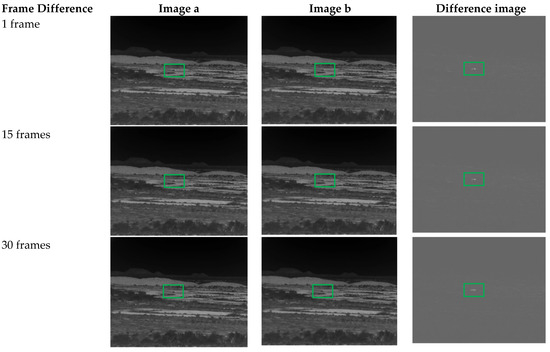
Figure 1.
Direct subtraction results. The frame separation needs to be large enough in order to detect moving objects.
2.2. Proposed Unsupervised Target Detection Approaches Using Change Detection
From Figure 1, the difference maps usually contain a lot of noise for a number of different reasons and the accurately detected change is still very dim. So, we tried using more sophisticated change detection algorithms. The three algorithms we tried are Covariance Equalization (CE) [35], Chronochrome (CC) [36], and Anomalous Change Detection (ACD) [37]. It should be noted that using change detection between two frames will also result in two detections. If these frames are far enough apart, there would be two vehicles present on the change detection map. In our experiments, a 15-frame gap between image pairs seems to create a reasonable balance where the vehicles overlap on the change detection map so there will only be one detection and the vehicles also create a reasonably sized detection due to the amount of separation that can occur in 15 frames. A smaller gap in frames has more overlap guaranteeing only one detection but creating a smaller detection as well. A larger gap in frames has a larger detection but increases the odds that there will be two changes detected rather than one.
The most effective workflow for tracking a moving target using change detection is to only use one frame every 15 frames and perform the following steps for each pair. The workflow of the standard approach is also illustrated in Figure 2 and the key steps are summarized below:
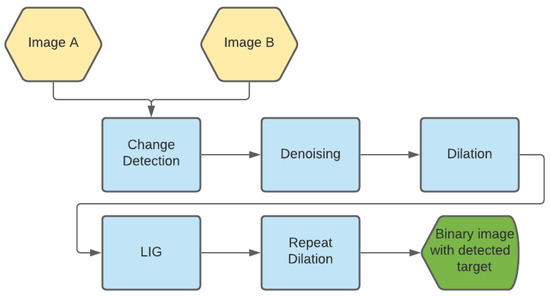
Figure 2.
Proposed standard approach to target detection.
- Perform change detection using a CD algorithm between two frames.
- Apply denoising to reduce the amount of noise in the change map.
- Perform dilation to increase size and intensity of detected changes
- Use LIG to detect anomalies in each change detection map.
- Perform dilation again to make detected change more visible
In Figure 3, we also show an alternative approach to target detection. The difference between the two approaches is the location of the LIG module. In the alternative approach, the LIG is applied to the two individual frames first. We will compare these two approaches in the experiments.
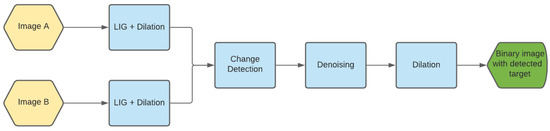
Figure 3.
Alternate approach to small target detection.
In the following paragraphs, we will briefly summarize the details of each module.
2.2.1. Change Detection
We have applied three change detection algorithms in our experiments.
Covariance Equalization (CE)
Suppose I(T1) is the reference (R) image and I(T2) is the test image (T). The algorithm is as follows [35]:
- 1.
- Compute mean and covariance of R and T as , , ,
- 2.
- Do eigen-decomposition (or SVD).
- 3.
- Do transformation.
- 4.
- The residual image between PR and PT is defined as
Chronochrome (CC)
Suppose I(T1) is the reference (R) image and a later image I(T2) the test image (T). The algorithm is as follows [36]:
- 1.
- Compute mean and covariance of R and T as , , ,
- 2.
- Compute cross-covariance between R and T as
- 3.
- Do transformation.
- 4.
- Compute the residual
Anomalous Change Detection (ACD)
ACD is a method of Anomalous Change detection created by Los Alamos National Laboratory [37]. ACD is based on an anomalous change detection framework that is applied to the Gaussian model. Suppose x and y are mean subtracted pixel vectors in two images (R and T) for the same pixel location. We denote the covariance of R and T as and
, and the cross-covariance between R and T as . The change value at pixel location (where x and y are) is then computed using
The change map is computed by applying Equation (6) for all pixels in R and T. In Equation (7), subscript R corresponds to the reference image, subscript T corresponds to the test image and Q is computed as
Different from Chronochrome (CC) and Covariance Equalization (CE) techniques, in ACD, the lines that separate normal from abnormal ones are hyperbolic.
2.2.2. Denoising
The denoising step is important in reducing speckle noise that could be detected as a change between two frames. During this step, Matlab’s imdiffusefilt function is used [47]. This function applies anisotropic diffusion filtering to denoise the change map.
2.2.3. Dilation
When using dilation, we used Matlab’s imdilate function using a disk with a size of 2 pixels as the parameter. This made the results from change detection much more clear. Figure 4 shows an example of its improvement.
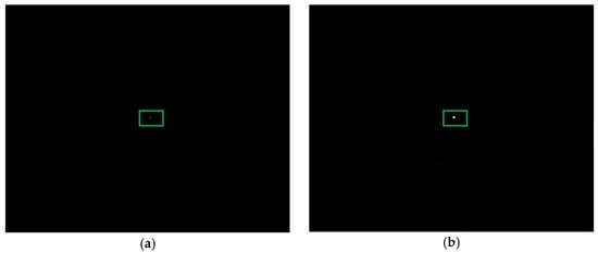
Figure 4.
Dilation results using a disk of size 2. (a) Raw frame; (b) Dilated frame.
2.2.4. LIG for Target Detection
Since the detection results of YOLO at the longer ranges (3500 m and above) were not as high as we would have liked, we also investigated a traditional unsupervised small target detection method to see how it would perform on the long range videos. The algorithm of choice for this study was a local intensity gradient (LIG) based target detector [5], specifically designed for infrared images. The LIG is relatively faster than other algorithms and is very robust to background clutter. Figure 5 highlights the architecture of the LIG [5]. The algorithm scans through the input image using a sliding window, whose size depends on the input image resolution. For each window, the local intensity and gradient values are computed separately. Then, those values are multiplied to form an intensity-gradient (IG) map. An adaptive threshold is then used to segment the IG map and then the binarized image will reveal the target.
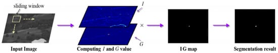
Figure 5.
Workflow of the LIG algorithm for small target detection.
A major advantage of these traditional/unsupervised algorithms is that they require no training, so there is no need to worry about customizing training data, which is the case with YOLO. A disadvantage of the LIG algorithm is that it is quite slow, taking roughly 70 s per frame.
There are two adjustments we made to the LIG algorithm to make it more suitable for the DSIAC infrared dataset. First of all, we adjusted the way in which the adaptable threshold T is calculated. One method to calculate T is to use the mean value of all non-zero pixels [5]. For our dataset, this calculation produced a very small value due to the overwhelming amount of very low non-zero pixels. The left image in Figure 6 highlights the significant role that the threshold plays for this algorithm. Second, we have implemented ways of speeding up the algorithm, such as incorporating multithreading within the script and also converting it to a faster interpreted language than MATLAB. We were able to speed up the computational time by close to three times.
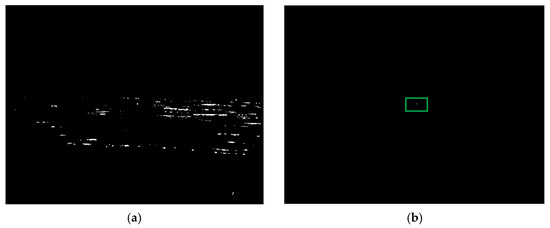
Figure 6.
Segmentation results using two different adaptive thresholds. (a) Original Adaptive Threshold [5]; (b) Our Adaptive Threshold.
For the example in Figure 6, the mean value was 0.008. Using this threshold value for binarization, we observe that roughly half the non-zero pixels would be considered as detections, as seen on the left hand image of Figure 6. This originally resulted in hundreds of false positives in the frames. So instead of using the mean of non-zero pixels in the LIG processed frame, we use the mean of the top 0.01% of pixels. A higher threshold is essential for eliminating false positives, as can be seen in the image on the right of Figure 6.
After running change detection using the CC method, the visual change maps appeared to be correct in most cases but there were a couple of pairs with a lot of noise. The LIG detection was able to clean up the noise in the pairs that performed poorly. Figure 7 below is an example of what these noisy frames looked like.
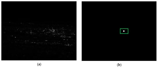
Figure 7.
Importance of LIG in small target detection. (a) Noisy change detection map; (b) LIG applied to noisy map.
2.2.5. Dilation Again after LIG
After LIG, dilation is again performed using a 10 × 10 pixel square as the parameter. Figure 8 shows an example of how this improves the visual result.
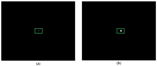
Figure 8.
Dilation results using a disk of size 10. (a) Raw; (b) Dilated.
2.2.6. Generation of Synthetic Bands
In the past, researchers have used EMAP to enhance change detection performance [38,39,40,41,42]. It was observed that EMAP can generate synthetic bands and improve the overall performance. As such, we considered using EMAP to improve the small target detection performance in infrared videos. EMAP allows us to convert a single band into a multispectral image made up of synthetic bands.
In another study, researchers also found that some synthetic bands using the LCE can help the target detection performance [43]. We implemented the LCE algorithm.
This section describes our attempts to expand this investigation.
EMAP
Mathematically, given an input grayscale image and a sequence of threshold levels , the attribute profile (AP) of is obtained by applying a sequence of thinning and thickening attribute transformations to every pixel in .
The EMAP of is then acquired by stacking two or more APs while using any feature reduction technique on multispectral/hyperspectral data, such as purely geometric attributes (e.g., area, length of the perimeter, image moments, shape factors), or textural attributes (e.g., range, standard deviation, entropy) [38,39,40,41].
In this paper, the “area (a)” and “length of the diagonal of the bounding box (d)” attributes of EMAP [42] were used. For the area attribute of EMAP, two thresholds used by the morphological attribute filters were set to 10 and 15. For the Length attribute of EMAP, the thresholds were set to 50, 100, and 500. The above thresholds were chosen based on experience, because we observed them to yield consistent results in our experiments. With this parameter setting, EMAP creates 11 synthetic bands for a given single band image. One of the bands comes from the original image.
LCE
LCE stands for Local Contrast Element [43]. This method of creating synthetic bands by creating a window around each pixel and finding the most similar pixels to the center. This method was used to create a varying number of bands. Figure 9 is a diagram explaining the logic in creating these synthetic bands.
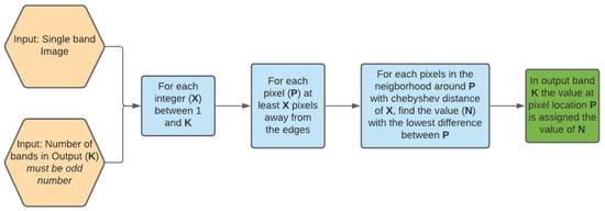
Figure 9.
LCE Workflow.
3. Experiments
3.1. Videos
Our research objective is to perform target detection in long range and low quality MWIR videos. There are no such datasets in the public domain except the DSIAC videos [47]. There are optical and MWIR videos in the DSIAC datasets. The optical and MWIR videos have very different characteristics. Optical imagers have a wavelength between 0.4 and 0.8 microns and MWIR imagers have a wavelength range between 3 and 5 microns. Optical cameras require external illuminations whereas MWIR counterparts do not need external illumination sources because MWIR cameras are sensitive to heat radiation from objects. Consequently, target shadows, illumination, and hot air turbulence can affect the target detection performance in optical videos. MWIR imagery is dominated by the thermal component at night and hence it is a much better surveillance tool than visible imagers at night. Moreover, atmospheric obscurants cause much less scattering in the MWIR bands than in the optical band. As a result, MWIR cameras are tolerant of heat turbulence, smoke, dust and fog. In this paper, we focused on the mid-wave infrared (MWIR) videos collected at distances ranging from 1000 m to 5000 m with 500 m increments. Each video has 1800 frames. The video frame rate is 7 frames/second and the frame size is 640 × 512. Each pixel is represented by 8 bits. These videos are challenging for several reasons. First, the target sizes are small due to long distances between the target and camera. This is quite different from some benchmark datasets such as the MOT Challenge [48] where the range from target to camera is short and the targets are big. Second, the target orientations also change drastically because the vehicles travel in a circle. Third, the illuminations in different videos are also different because of changes in cloud cover and time of day. Fourth, the cameras also move in some videos.
3.2. Performance Metrics
A correct detection or true positive (TP) occurs if the binarized detection is within a certain threshold of the centroid of the ground truth bounding box. Otherwise, the detected object is regarded as a false positive (FP). If a frame does not have a TP, then a missed detection (MD) occurs. Based on the correct detection and false positive counts, we can further generate precision, recall, and F1 metrics. The precision (P), recall (R), and F1 are defined as
3.3. Experiments to Demonstrate the Proposed Frameworks
In this section, we will include some experimental results to illustrate the importance of some critical modules. Figure 10 shows a few frames in the 3500 m video (daytime) even though the frames look very dark.
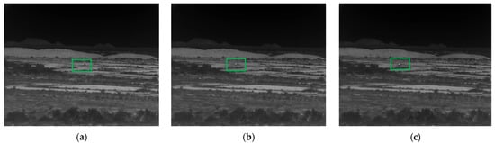
Figure 10.
Frames from the 3500 m video. (a) Frame 1; (b) Frame 900; (c) Frame 1800.
3.3.1. Baseline Performance Using Direct Subtraction
Although the results shown in Figure 1 appear to show that we are able to detect the moving target using direct subtraction, there are actually many false positives in different places. In order to quantify the performance of direct subtraction, we performed several experiments by using 300 frame pairs in the 3500 m videos.
Here, we briefly mention how we generated the 300 frame pairs. For every five frames, we would select a pre-image and the corresponding post-image would be the 15th frame after the pre-image.
The first experiment was to perform direct subtraction without any other processing steps in the workflows. Table 1 summarizes the results. One can see that the false positives are vast and greatly outnumber the true positives. In the second experiment, we performed change detection by using direct subtraction in the standard workflow as shown in Figure 2. It should be noted that the workflow remains the same except for the change detection module in which a direct subtraction was performed. The detection results are shown in Table 2. It can be seen that direct subtraction worked quite well. In the third experiment, we excluded the LIG module in the standard workflow. The results are shown in Table 3. We can see that the performance dropped quite significantly. This means that the LIG module plays an important role in the workflow.

Table 1.
Direct subtraction results using 300 frame pairs without subsequent processing steps.
Table 2.
Detection results from using direct subtraction to generate change maps with full standard workflow. 300 frame pairs are used.
Table 3.
Direct subtraction with full standard workflow excluding LIG. 300 frame pairs are used.
3.3.2. Importance of LIG in the Full Standard and Alternative Workflows
From Section 3.3.1, we observed that LIG played a very important role in object detection when simple direct subtraction was used for change detection. It will be important to demonstrate the importance of LIG in the full workflows containing more sophisticated change detection algorithms. When there is no LIG, the two workflows are actually the same. In the change detection module, we have compared three change detection algorithms. We performed an experiment using 300 frame pairs in the 3500 m video.
Table 4 shows the detection results without using LIG. It can be seen that there are more than one detection per frame and a lot of false positives. This is similar to Table 3 where a direct subtraction was performed. Comparing Table 3 and Table 4, we can observe the following. First, ACD has the fewest false positives in this case. Second, all three change detection methods performed better (fewer FP) than direct subtraction.
Table 4.
Detection results of the standard/alternate approaches excluding LIG. 300 frame pairs were used. Bold numbers indicate the best performing method in each column.
Table 5 summarizes the results with LIG in the standard workflow and the alternative workflow, respectively. We can see that the standard approach performed much better than the alternate approach. In the alternate approach, there are simply more false positives. We think that one possible reason for better results in the standard flow is because of the location of the LIG in the workflow. It should be noted that the LIG contains an adaptive thresholding step. In the standard workflow, this thresholding is done in the later stage whereas the LIG is applied in the early stage in the alternative workflow. We believe that, since the thresholding is a hard decision step, a wrong decision in the thresholding may cause some additional wrong decisions in the subsequent steps. Hence, it is better to delay the thresholding in the later stage of the workflow.
Table 5.
Detection results from the Standard and Alternate approaches with LIG. There is a 15 frame separation. 300 frame pairs were used. Bold numbers indicate the best performing method in each column.
3.3.3. Detection Results for 4000 m and 5000 m Videos
Here, we will summarize additional experiments using videos from 4000 m and 5000 m ranges using the full standard and alternate workflow. Figure 11 shows a few frames from the raw 4000 m video. The target sizes are quite small and it is hard to visually see any potential targets in the scene. Table 6 summarizes the detection results using the standard and alternate workflows. It can be seen that the standard approach has much fewer false positives in two out of three cases. Moreover, in the 4000 m video, the CC and CE performed slightly better than ACD.
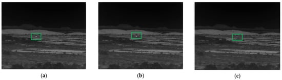
Figure 11.
Frames from the 4000 m video. (a) Frame 1; (b) Frame 900; (c) Frame 1800.
Table 6.
Detection results from the Standard and Alternate approaches with a 15 frame separation where the target is at 4000 m. 300 frame pairs were used. Bold numbers indicate the best performing method in each column.
Figure 12 shows a few frames from the 5000 m video. The target size is even small than other ranges. Table 7 summarizes the detection results using the standard and alternate workflows. One can observe that there are more false positives and missed detection. This is understandable as the target size is so small. Moreover, we can see that the standard workflow performed better than the alternate workflow in two out of three cases. However, the alternative workflow has better results in the CC case.
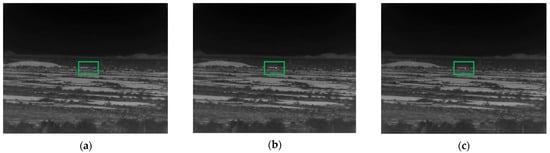
Figure 12.
Frames from the 5000 m video. (a) Frame 1; (b) Frame 900; (c) Frame 1800.
Table 7.
Detection results from the Standard and Alternate approach with a 15 frame separation where the target is at 5000 m. Bold numbers indicate the best performing method in each column.
3.3.4. Additional Investigations Using EMAP and LCE
Here, we summarize and compare the detection results using synthetic and original bands. The videos range from 3500 m to 5000 m.
Results for the 3500 m Video
As shown in Table 8, the results when using the single band original image are significantly stronger than the synthetic bands especially when compared against EMAP.
Table 8.
Detection results of the standard approach with 15 frame separation comparing the single band approach to the multi band synthetic approach. The target is at a distance of 3500 m. LCE5 has 5 bands. EMAP has 11 bands. Bold numbers indicate the best performing method in each column.
Table 8 shows the results from those two experiments. In LCE5, there are 5 bands. In every case, the single band approach is stronger at 3500 m.
Results for the 4000 m Video
The results below are created using the standard approach. As shown in Table 9, the detection results at 4000 m were very good for all cases. We also observe that the EMAP results with ACD and CE are comparable to those using the original video.
Table 9.
Detection results of the standard approach with 15 frame separation using the original single band frames. The target is at a distance of 4000 m. LCE5 has 5 bands. EMAP has 11 bands. Bold numbers indicate the best performing method in each column.
Results for the 5000 m Video
As shown in Table 10, the single band approach had 10 false detections for all three CD methods. The EMAP performed slightly worse, especially with the CC change detection method. The LCE5 approach with ACD and CE shows improvement over the single band case. In order to find improvements with EMAP, we tried modifying the vector value and the attribute value but no changes to those values show any significant improvement.
Table 10.
Detection results of the standard approach with 15 frame separation. The target is at a distance of 5000 m. LCE5 has 5 bands. EMAP has 11 bands. Bold numbers indicate the best performing method in each column.
3.3.5. Subjective Results
Figure 13, Figure 14 and Figure 15 show some detection results for the three long ranges. Since the detection involves two frames, we denote the current frame as the reference frame. The other frame is 15 frames before the reference frame. The ground truth target location, correct detection location, and false position location are overlaid to the reference frame. A green box highlights a true detection. A blue box highlights the ground truth bounding box and a red box highlights a false positive.
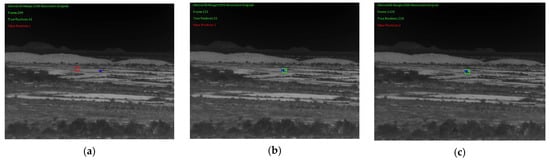
Figure 13.
Exemplar detection results for 3500 m video using the standard approach. Ground truth, correct detection, and false positives are overlaid onto the reference frames. (a) Reference frame 249; (b) Reference frame 333; (c) Reference frame 1329.
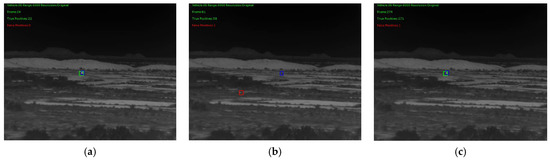
Figure 14.
Exemplar detection results for 4000 m video using the standard approach. (a) Reference frame 24; (b) Reference frame 61; (c) Reference frame 274.
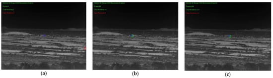
Figure 15.
Exemplar detection results for 5000 m video using the standard approach. (a) Reference frame 6; (b) Reference frame 39; (c) Reference frame 289.
3.3.6. Computational Times
As can be seen in Table 11, the most time-consuming module in the standard approach is the LIG module, which takes about 70 s per frame. For the alternate approach, there are two LIG modules and hence it takes 140 s per frame pair. Since the bottleneck is LIG, there are several potential methods to speed up the processing of LIG that can be done in the future. First, since LIG is a local approach that performs object detection window by window, one feasible approach is to apply a graphical processor unit (GPU) to speed up the process. In a typical GPU, there are several thousand processors. If done properly, each processor can handle a small window. Consequently, significant speed up can be achieved. Second, one can also analyze the LIG algorithm closely and see if one can optimize the implementation. Third, if one needs to implement LIG in hardware, then field programmable gate array (FPGA) can be utilized. Based on our understanding, FPGA can also execute parallel processing tasks.
Table 11.
Computational times per frame pair of the two workflows.
3.3.7. Performance Comparison with Other Approaches
Here, we compare the performance of the proposed algorithm (standard workflow containing the CC change detection method) with two other conventional algorithms. One conventional algorithm is based on frame by frame detection [7] and the other one is based on optical flow [34]. Details can be found in [7,34]. Table 12 summarizes the detection metrics for 3500 m, 4000 m, and 5000 m videos. One can see that the proposed method has comparable or better detection results than the two other methods.
Table 12.
Comparison of the proposed algorithm with two conventional algorithms. Bold numbers indicate the best performing method in each column.
4. Conclusions
In this paper, we presented two approaches for small moving target detection in long range infrared videos. Both approaches are unsupervised, modular, and flexible frameworks. The frameworks were motivated by change detection algorithms in remote sensing. It was observed that change detection algorithms performed better than direct subtraction. Another observation is that the standard approach performed better than the alternate approach in most cases. The most influential module is the LIG detection module, which can detect small targets quite effectively. We also experimented with synthetic band generation algorithms. We have seen some positive impacts in longer ranges such as 4000 m and 5000 m videos.
One limitation of the current approaches is that the computational time is too long. Fast implementation using GPU and FPGA will be explored in the near future. It is also noted that there are some recent advances in target detection in remote sensing images [49,50,51] that may have great potential in infrared images/videos.
Author Contributions
Conceptualization, C.K.; methodology, C.K.; software, J.L.; validation, C.K. and J.L.; resources, C.K.; data curation, C.K.; writing—original draft preparation, C.K.; writing—review and editing, C.K.; supervision, C.K.; project administration, C.K.; funding acquisition, C.K. All authors have read and agreed to the published version of the manuscript.
Funding
This work was partially supported by US government PPP program. The views, opinions and/or findings expressed are those of the author(s) and should not be interpreted as representing the official views or the U.S. Government.
Institutional Review Board Statement
Not applicable.
Informed Consent Statement
Not applicable.
Data Availability Statement
Not applicable.
Conflicts of Interest
The authors declare no conflict of interest.
References
- Chen, C.L.P.; Li, H.; Wei, Y.; Xia, T.; Tang, Y.Y. A Local Contrast Method for Small Infrared Target Detection. IEEE Trans. Geosci. Remote Sens. 2014, 52, 574–581. [Google Scholar] [CrossRef]
- Wei, Y.; You, X.; Li, H. Multiscale patch-based contrast measure for small infrared target detection. Pattern Recognit. 2016, 58, 216–226. [Google Scholar] [CrossRef]
- Gao, C.; Meng, D.; Yang, Y.; Wang, Y.; Zhou, X.; Hauptmann, A.G. Infrared Patch-Image Model for Small Target Detection in a Single Image. IEEE Trans. Image Process. 2013, 22, 4996–5009. [Google Scholar] [CrossRef]
- Zhang, L.; Peng, L.; Zhang, T.; Cao, S.; Peng, Z. Infrared Small Target Detection via Non-Convex Rank Approximation Minimization Joint l2,1 Norm. Remote Sens. 2018, 10, 1821. [Google Scholar] [CrossRef] [Green Version]
- Zhang, H.; Zhang, L.; Yuan, D.; Chen, H. Infrared small target detection based on local intensity and gradient properties. Infrared Phys. Technol. 2018, 89, 88–96. [Google Scholar] [CrossRef]
- Chen, Y.; Zhang, G.; Ma, Y.; Kang, J.U.; Kwan, C. Small Infrared Target Detection Based on Fast Adaptive Masking and Scaling with Iterative Segmentation. IEEE Geosci. Remote Sens. Lett. 2021, 1–5. [Google Scholar] [CrossRef]
- Kwan, C.; Budavari, B. A high-performance approach to detecting small targets in long-range low-quality infrared videos. Signal Image Video Process. 2021, 1–9. [Google Scholar] [CrossRef]
- Demir, H.S.; Cetin, A.E. Co-difference based object tracking algorithm for infrared videos. In Proceedings of the 2016 IEEE International Conference on Image Processing (ICIP), Phoenix, AZ, USA, 25–28 September 2016; pp. 434–438. [Google Scholar]
- Kwan, C.; Gribben, D. Importance of training strategies on target detection performance using deep learning algorithms in long range infrared videos. Signal Image Process. Int. J. 2021, 12, 3. [Google Scholar]
- Kwan, C.; Gribben, D.; Budavari, B. Target Detection and Classification Performance Enhancement using Super-Resolution Infrared Videos. Signal Image Process. Int. J. 2021, 12, 33–45. [Google Scholar] [CrossRef]
- Kwan, C.; Gribben, D. Target Detection and Classification Improvements using Contrast Enhanced 16-bit Infrared Videos. Signal Image Process. Int. J. 2021, 12, 23–38. [Google Scholar] [CrossRef]
- Kong, X.; Yang, C.; Cao, S.; Li, C.; Peng, Z. Infrared Small Target Detection via Nonconvex Tensor Fibered Rank Approximation. IEEE Trans. Geosci. Remote Sens. 2021, 1–21. [Google Scholar] [CrossRef]
- Kwan, C.; Chou, B.; Yang, J.; Tran, T. Deep Learning Based Target Tracking and Classification Directly in Compressive Measurement for Low Quality Videos. Signal Image Process. Int. J. 2019, 10, 9–29. [Google Scholar] [CrossRef]
- Ma, D.; Dong, L.; Xu, W. A Method for Infrared Sea-Sky Condition Judgment and Search System: Robust Target Detection via PLS and CEDoG. IEEE Access 2021, 9, 1439–1453. [Google Scholar] [CrossRef]
- Dai, Y.; Wu, Y.; Zhou, F.; Barnard, K. Attentional Local Contrast Networks for Infrared Small Target Detection. IEEE Trans. Geosci. Remote Sens. 2021, 1–12. [Google Scholar] [CrossRef]
- Yang, P.; Dong, L.; Xu, W. Infrared Small Maritime Target Detection Based on Integrated Target Saliency Measure. IEEE J. Sel. Top. Appl. Earth Obs. Remote Sens. 2021, 14, 2369–2386. [Google Scholar] [CrossRef]
- Pang, D.; Shan, T.; Ma, P.; Li, W.; Liu, S.; Tao, R. A Novel Spatiotemporal Saliency Method for Low-Altitude Slow Small Infrared Target Detection. IEEE Geosci. Remote Sens. Lett. 2021, 1–5. [Google Scholar] [CrossRef]
- Hou, Q.; Wang, Z.; Tan, F.; Zhao, Y.; Zheng, H.; Zhang, W. RISTDnet: Robust Infrared Small Target Detection Network. IEEE Geosci. Remote Sens. Lett. 2021, 1–5. [Google Scholar] [CrossRef]
- Du, S.; Zhang, P.; Zhang, B.; Xu, H. Weak and Occluded Vehicle Detection in Complex Infrared Environment Based on Improved YOLOv4. IEEE Access 2021, 9, 25671–25680. [Google Scholar] [CrossRef]
- Song, Z.; Yang, J.; Zhang, D.; Wang, S.; Li, Z. Semi-Supervised Dim and Small Infrared Ship Detection Network Based on Haar Wavelet. IEEE Access 2021, 9, 29686–29695. [Google Scholar] [CrossRef]
- Wan, M.; Ye, X.; Zhang, X.; Xu, Y.; Gu, G.; Chen, Q. Infrared Small Target Tracking via Gaussian Curvature-Based Compressive Convolution Feature Extraction. IEEE Geosci. Remote Sens. Lett. 2021, 1–5. [Google Scholar] [CrossRef]
- Zhao, M.; Li, W.; Li, L.; Ma, P.; Cai, Z.; Tao, R. Three-Order Tensor Creation and Tucker Decomposition for Infrared Small-Target Detection. IEEE Trans. Geosci. Remote Sens. 2021, 1–16. [Google Scholar] [CrossRef]
- Sun, H.; Liu, Q.; Wang, J.; Ren, J.; Wu, Y.; Zhao, H.; Li, H. Fusion of Infrared and Visible Images for Remote Detection of Low-Altitude Slow-Speed Small Targets. IEEE J. Sel. Top. Appl. Earth Obs. Remote Sens. 2021, 14, 2971–2983. [Google Scholar] [CrossRef]
- Raza, A.; Liu, J.; Liu, Y.; Liu, J.; Li, Z.; Chen, X.; Huo, H.; Fang, T. IR-MSDNet: Infrared and Visible Image Fusion Based On Infrared Features and Multiscale Dense Network. IEEE J. Sel. Top. Appl. Earth Obs. Remote Sens. 2021, 14, 3426–3437. [Google Scholar] [CrossRef]
- Xue, W.; Qi, J.; Shao, G.; Xiao, Z.; Zhang, Y.; Zhong, P. Low-Rank Approximation and Multiple Sparse Constraint Modeling for Infrared Low-Flying Fixed-Wing UAV Detection. IEEE J. Sel. Top. Appl. Earth Obs. Remote Sens. 2021, 14, 4150–4166. [Google Scholar] [CrossRef]
- Lohit, S.; Kulkarni, K.; Turaga, P. Direct inference on compressive measurements using convolutional neural networks. In Proceedings of the 2016 IEEE International Conference on Image Processing, Phoenix, AZ, USA, 25–28 September 2016; pp. 1913–1917. [Google Scholar] [CrossRef]
- Adler, A.; Elad, M.; Zibulevsky, M. Compressed Learning: A Deep Neural Network Approach. arXiv 2016, arXiv:1610.09615v1. [Google Scholar]
- Xu, Y.; Kelly, K.F. Compressed domain image classification using a multi-rate neural network. arXiv 2019, arXiv:1901.09983. [Google Scholar]
- Wang, Z.W.; Vineet, V.; Pittaluga, F.; Sinha, S.N.; Cossairt, O.; Kang, S.B. Privacy-Preserving Action Recognition Using Coded Aperture Videos. In Proceedings of the 2019 IEEE/CVF Conference on Computer Vision and Pattern Recognition Workshops (CVPRW), Long Beach, CA, USA, 16–17 June 2019; pp. 1–10. [Google Scholar]
- Vargas, H.; Fonseca, Y.; Arguello, H. Object Detection on Compressive Measurements using Correlation Filters and Sparse Representation. In Proceedings of the 2018 26th European Signal Processing Conference (EUSIPCO), Rome, Italy, 3–7 September 2018; pp. 1960–1964. [Google Scholar]
- Degerli, A.; Aslan, S.; Yamac, M.; Sankur, B.; Gabbouj, M. Compressively Sensed Image Recognition. In Proceedings of the 2018 7th European Workshop on Visual Information Processing (EUVIP), Tampere, Finland, 26–28 November 2018; pp. 1–6. [Google Scholar]
- Latorre-Carmona, P.; Traver, V.J.; Sánchez, J.S.; Tajahuerce, E. Online reconstruction-free single-pixel image classification. Image Vis. Comput. 2019, 86, 28–37. [Google Scholar] [CrossRef]
- Kwan, C.; Gribben, D.; Chou, B.; Budavari, B.; Larkin, J.; Rangamani, A.; Tran, T.; Zhang, J.; Etienne-Cummings, R. Real-Time and Deep Learning Based Vehicle Detection and Classification Using Pixel-Wise Code Exposure Measurements. Electronics 2020, 9, 1014. [Google Scholar] [CrossRef]
- Kwan, C.; Budavari, B. Enhancing Small Moving Target Detection Performance in Low-Quality and Long-Range Infrared Videos Using Optical Flow Techniques. Remote Sens. 2020, 12, 4024. [Google Scholar] [CrossRef]
- Schaum, A.P.; Stocker, A. Hyperspectral change detection and supervised matched filtering based on covariance equalization. Def. Secur. 2004, 5425, 77–90. [Google Scholar] [CrossRef]
- Schaum, A.; Stocker, A. Long-interval chronochrome target detection. Int. Symp. Spectral Sens. Res. 1997, 1760–1770. [Google Scholar]
- Theiler, J.; Perkins, S. Proposed framework for anomalous change detection. In ICML Workshop on Machine Learning Algorithms for Surveillance and Event Detection; Association for Computing Machinery: New York, NY, USA, 2006. [Google Scholar]
- Bernabe, S.; Marpu, P.R.; Plaza, A.; Mura, M.D.; Benediktsson, J.A. Spectral–Spatial Classification of Multispectral Images Using Kernel Feature Space Representation. IEEE Geosci. Remote Sens. Lett. 2013, 11, 288–292. [Google Scholar] [CrossRef]
- Bernabé, S.; Marpu, P.R.; Plaza, A.; Benediktsson, J.A. Spectral unmixing of multispectral satellite images with dimensionality expansion using morphological profiles. In Proceedings of the Satellite Data Compression, Communications, and Processing VIII, San Diego, CA, USA, 19 October 2012; Volume 8514, p. 85140Z. [Google Scholar]
- Mura, M.D.; Benediktsson, J.A.; Waske, B.; Bruzzone, L. Morphological Attribute Profiles for the Analysis of Very High Resolution Images. IEEE Trans. Geosci. Remote Sens. 2010, 48, 3747–3762. [Google Scholar] [CrossRef]
- Mura, M.D.; Benediktsson, J.A.; Waske, B.; Bruzzone, L. Extended profiles with morphological attribute filters for the analysis of hyperspectral data. Int. J. Remote Sens. 2010, 31, 5975–5991. [Google Scholar] [CrossRef]
- Dao, M.; Kwan, C.; Bernabe, S.; Plaza, A.J.; Koperski, K. A Joint Sparsity Approach to Soil Detection Using Expanded Bands of WV-2 Images. IEEE Geosci. Remote Sens. Lett. 2019, 16, 1869–1873. [Google Scholar] [CrossRef]
- Xia, C.; Li, X.; Zhao, L. Infrared Small Target Detection via Modified Random Walks. Remote Sens. 2018, 10, 2004. [Google Scholar] [CrossRef] [Green Version]
- Ayhan, B.; Kwan, C. A New Approach to Change Detection Using Heterogeneous Images. In Proceedings of the 2019 IEEE 10th Annual Ubiquitous Computing, Electronics & Mobile Communication Conference (UEMCON), New York, NY, USA, 10–12 October 2019. [Google Scholar]
- Kwan, C.; Zhou, J. High performance change detection in hyperspectral images using multiple references. In Proceedings of the Algorithms and Technologies for Multispectral, Hyperspectral, and Ultraspectral Imagery XXIV, Orlando, FL, USA, 15–19 April 2018; Volume 10644, p. 106440Z. [Google Scholar]
- DSIAC Dataset. Available online: https://blogs.upm.es/gti-work/2013/05/06/sensiac-dataset-for-automatic-target-recognition-in-infrared-imagery/ (accessed on 16 August 2021).
- Mathworks. 2020. Available online: https://www.mathworks.com/help/images/ref/imdiffusefilt.html (accessed on 6 July 2021).
- MOT Challenge. Available online: https://motchallenge.net/ (accessed on 6 July 2021).
- Li, K.; Wan, G.; Cheng, G.; Meng, L.; Han, J. Object detection in optical remote sensing images: A survey and a new benchmark. ISPRS J. Photogramm. Remote Sens. 2020, 159, 296–307. [Google Scholar] [CrossRef]
- Li, K.; Cheng, G.; Bu, S.; You, X. Rotation-Insensitive and Context-Augmented Object Detection in Remote Sensing Images. IEEE Trans. Geosci. Remote Sens. 2018, 56, 2337–2348. [Google Scholar] [CrossRef]
- Cheng, G.; Zhou, P.; Han, J. Learning Rotation-Invariant Convolutional Neural Networks for Object Detection in VHR Optical Remote Sensing Images. IEEE Trans. Geosci. Remote Sens. 2016, 54, 7405–7415. [Google Scholar] [CrossRef]
Publisher’s Note: MDPI stays neutral with regard to jurisdictional claims in published maps and institutional affiliations. |
© 2021 by the authors. Licensee MDPI, Basel, Switzerland. This article is an open access article distributed under the terms and conditions of the Creative Commons Attribution (CC BY) license (https://creativecommons.org/licenses/by/4.0/).