Abstract
We present a theoretical study of the nonlinear dynamics of a long external cavity delayed optical feedback-induced interband cascade laser (ICL). Using the modified Lang–Kobayashi equations, we numerically investigate the effects of some key parameters on the first Hopf bifurcation point of ICL with optical feedback, such as the delay time (τf), pump current (I), linewidth enhancement factor (LEF), stage number (m) and feedback strength (fext). It is found that compared with τf, I, LEF and m have a significant effect on the stability of the ICL. Additionally, our results show that an ICL with few stage numbers subjected to external cavity optical feedback is more susceptible to exhibiting chaos. The chaos bandwidth dependences on m, I and fext are investigated, and 8 GHz bandwidth mid-infrared chaos is observed.
1. Introduction
As a mid-infrared semiconductor laser, the interband cascade laser (ICL) has made significant progress in the last two decades [1,2,3,4,5,6]. The RAND Corporation reports that mid-infrared lasers in the 3–5 μm band of the atmospheric transmission window have good atmospheric transmission characteristics, lower transmission losses than other bands, and are less susceptible to weather factors [7]. In addition, the mid-infrared band covers the absorption peaks of many atoms and molecules [8]. Therefore, ICL can be used in applications such as gas detection [9,10], clinical respiratory diagnosis [11] and free-space optical communication [12].
In contrast to the quantum cascade laser (QCL), the ICL is a bipolar device, with the electronic transition of the ICL occurring between the conduction and the valence sub-bands [13]. Therefore, the carrier lifetime of the ICL is in the nanosecond order like in more conventional semiconductor lasers. Furthermore, in recent experimental reports the linewidth enhancement factor of the ICL was found to be about 2.2, which is much higher than that of QCL [14,15]. Both of these characteristics suggest that when subjected to external perturbation, the ICL will exhibit rich nonlinear dynamics. Wang et al.’s recent experiments confirm that with external optical feedback the ICL exhibits periodic oscillations and weak chaos [16]. 450 MHz low frequency oscillation (detector bandwidth limited) chaos was observed. However, the route to chaos and the identification of the means for obtaining strong chaos are open for detailed study. A recent report shows that based on a QCL with external optical feedback, a generated mid-infrared low frequency chaotic oscillation was used to achieve 0.5 Mbit/s message private free-space optical communication [17]. To realize a much higher-speed message secure transmission, strong broadband chaos is essential.
In this paper, modified Lang–Kobayashi equations are used to investigate the dynamics of the ICL subject to external optical feedback. ICLs with short external cavities have been used to affect wavelength tuning [18]. In contrast, and with a view to performing experiments with discrete devices [19,20,21,22,23,24,25], we focus on the case of optical feedback from longer external cavities, wherein the external feedback delay time is larger than the oscillation relaxation time of the ICL [26]. The pump current, feedback strength, stage number and linewidth enhancement factor effects on the stability of the ICL with optical feedback are analyzed, and the influence of the stage number, pump current and feedback strength on the bandwidth of chaos are investigated.
2. Theoretical Model
Figure 1a presents an ICL structure having three stages. Initially, the electron transition in the ICL occurs between the first conduction sub-band and the first valence sub-band, as indicated as Ee (blue potential well) and Eh (red potential well) in the left upper corner in Figure 1a [27]. After the first electron transition, the electron reaches the second stage conduction sub-band through interband tunneling and then repeats the electron transition in the second stage and then in the third stage. Figure 1b is the schematic diagram of an ICL subjected to external mirror feedback, where τf is the feedback time delay.

Figure 1.
(a) 3-stage number structure of interband cascade laser(ICL); (b) Schematic diagram of ICL with optical feedback structure.
Using appropriately modified Lang–Kobayashi equations, the rate equations for the ICL with optical feedback are as follows [28,29]:
where N(t), S(t) and φ(t) respectively represent the per stage carrier number, total photon number of all gain stages and phase of the electric field. M is the number of gain stages, τsp is the spontaneous radiation lifetime, and τaug is the Auger recombination lifetime. Since the Auger recombination lifetime τaug in the ICL is smaller than the spontaneous radiation lifetime τsp, τaug must be considered in the current-carrying dynamics. In principle, the Auger coefficient has a carrier density dependence, as in ref. [30]. In this work, we follow [29] in assuming a constant value for the Auger lifetime. η is the current injection efficiency, Γp is the optical confinement factor per gain stage, νg is the group velocity of light, g is the material gain per stage which is given by g = a0[N(t) − Ntr]/A. τp is the photon lifetime, and k is the feedback coefficient which is given by , where τin is the internal cavity roundtrip time, fext is the feedback strength which is defined as the power ratio between the feedback light and the laser output, and Cl is an external coupling coefficient. The external coupling coefficient can be expressed as , with R being the reflection coefficient of the laser front facet facing the external mirror.
The steady-state solutions for the ICL operating above the threshold current are as follows [29]:
The descriptions of other symbols and their values used in the simulation are given in Table 1, as taken from [14,27,29,30,31,32]. The integration time step in the simulation is 0.1 ps.

Table 1.
ICL parameters used in the simulations.
3. Numerical Results
We calculate the carrier number and photon number for an increasing bias current, as shown in Figure 2a,b, respectively. It is found that the number of stages m has little effect on the carrier number (in Figure 2a) but that it influences the photon number (in Figure 2b). For relatively large numbers of stages such as m = 10 (red dashed curve), the output power is much higher than in the case of m = 5 (black solid curve), as shown in Figure 2b.
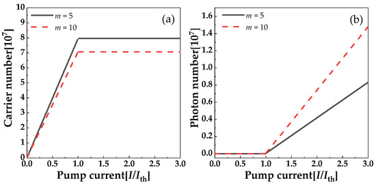
Figure 2.
(a) Carrier number and (b) photon number vs. pump current. Black solid and red dashed curves represent stage numbers m = 5 and m = 10, respectively.
3.1. Route to Chaos
Figure 3 shows the output of the ICL with external optical feedback as the feedback strength increases, for the case of m = 5. The ICL output is stable when the feedback strength fext ranges from 0 to 0.019%. Without feedback, that is fext = 0, the relaxation oscillation frequency fR can be observed from the RF spectrum in Figure 3(d-i) to be 1.02 GHz. This is in accordance with the value 1.035 GHz obtained by calculating the relaxation oscillation frequency via the relation fR = (G0S0/τp)−1/2/(2π), where G0 = Γpvga0/A and S0 are found from Equation (5). As the feedback strength increases, the ICL enters into period-1 dynamics (ii), quasi-periodic dynamics (iii), weak chaos oscillations (iv), and then displays strong chaos (v). The frequency of period-1 oscillations is 1.03 GHz, as shown in Figure 3(d-ii), which is a little larger than the relaxation oscillation frequency shown in Figure 3(a-ii). As the feedback strength increases, a quasi-periodic oscillation is found, which is confirmed by the RF spectrum and phase diagram; that is, more frequencies are induced in Figure 3(d-iii) and more loops are found in the phase in Figure 3(c-iii), respectively. An irregular laser intensity oscillation is observed where the ICL enters into weak chaos, as shown in Figure 3(a-iv). Although the highest peak in the RF spectrum is still at 1.03 GHz, more frequency components appear, as presented in Figure 3(d-iv). For a further increase in the feedback strength, more complex nonlinear dynamics are introduced, hence achieving strong mid-infrared optical chaos, as shown in Figure 3(a-v–e-v). In the optical spectra of the chaos shown in Figure 3(e-v), many external cavity modes with a frequency interval around 410 MHz are found. This can be confirmed from the auto-correlation functions shown in Figure 3(b-v), where the sidelobe peak is at 2.4 ns, corresponding to a cavity length of 36 cm.
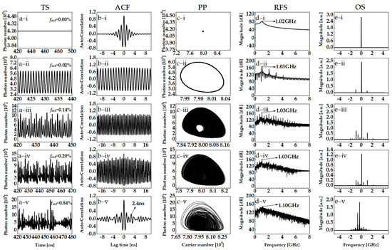
Figure 3.
Output of ICL with external optical feedback as feedback strength increases with m = 5, I = 1.1Ith, and τf = 2.4 ns; from the top down, i: fext = 0.0%, ii: fext = 0.02%, iii: fext = 0.14%, iv: fext = 0.20%, v: fext = 0.84%; columns (a–e) are time series (TS), autocorrelation curve functions (ACF), phase portrait (PP), radio-frequency spectrum (RFS) and optical spectra (OS), respectively.
By using bifurcation diagrams, the dynamics of the ICL for increasing feedback strength can be obtained, as shown in Figure 4(a-i) with m = 5 and Figure 4(b-i) with m = 10. Maximum Lyapunov exponents [33,34] can be used to determine whether the ICL output with external optical feedback is chaotic (red dots) or not (blue dots), as shown in Figure 4(a-ii,b-ii). As shown in Figure 4(a-i), the route to chaos for a 10-stage ICL with external optical feedback is from stable (S) to period-1 (P1), then quasi-periodic (QP) and then chaos (C). This route is different from that of a 10-stage ICL where multiple-periodic (MP) oscillations are observed. The number of stages m has an effect on the photon number and phase, as presented in Equations (2) and (3), which results in different routes to chaos.
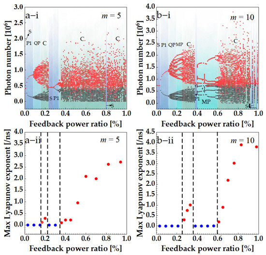
Figure 4.
Bifurcations (i) and Maximum Lyapunov exponents (ii) of ICL output with external optical feedback under I = 1.1Ith, τf = 2.4 ns. (a) m = 5, (b) m = 10.
3.2. Hopf Bifurcation Analysis
In this section, we explore the stability of ICLs with external optical feedback. We first compare two stage numbers, which are m = 5 and m = 10, to reveal the effects of the time delay, bias current and linewidth enhancement factor on the Hopf bifurcation points. Then, we ascertain how the Hopf bifurcation changes for stage numbers m in the range of 3 to 20.
The pump current is set a little above the threshold current, that is 1.1Ith. Figure 5 shows that the external cavity delay has little effect on the Hopf bifurcation point. As the external cavity delay increases from 1.5 ns to 5.0 ns, the Hopf bifurcation point values, that is the feedback power ratio where the ICL enters into P1, are around 0.02% to 0.33%. As shown in Figure 5, there is a periodic dependence of the Hopf bifurcation point on the external cavity delay time; for a 2.1 ns delay time, the value of the Hopf bifurcation point reaches a maximum and the second peak is at 3.0 ns. As the delay time increases, the differences between the Hopf bifurcation points reduce.
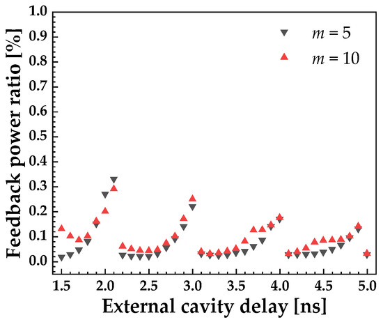
Figure 5.
Hopf bifurcation point vs. time delay τf for I = 1.1Ith.
To illustrate the pump current effects, the dependence of the Hopf bifurcation point on bias current is investigated. In Figure 6a,b, two external cavity delays are compared, viz τf = 2.0 ns and τf = 2.4 ns. As the pump current increases, the Hopf bifurcation point gradually increases for both m = 5 (squares) and m = 10 (circles) cases, as well as for τf = 2.0 ns and τf = 2.4 ns. Compared with τf = 2.4 ns, at τf = 2.0 ns there is a need for a larger feedback power ratio to enable the ICL to enter an unstable state, which is around 1.3 times that of τf = 2.4 ns for a pump current of 3Ith. Since these two delays show similar trends for the Hopf bifurcation point versus bias current, we focus our attention on τf = 2.4 ns in the following results.
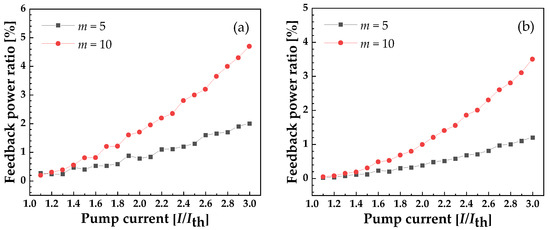
Figure 6.
Hopf bifurcation point vs. bias current. (a) τf = 2.0 ns, (b) τf = 2.4 ns.
It is well-appreciated that the linewidth enhancement factor, αH, plays a crucial role in semiconductor laser nonlinear dynamics. For common quantum well laser diodes, αH is in the range of 2.0 to 5.0 [35,36]. A recent report shows that the below-threshold linewidth enhancement factor of ICL is in the range of 1.1–1.4 [14]. Here, we calculate the Hopf bifurcation point versus linewidth enhancement factor, which ranges from 1 to 5, as shown in Figure 7. As the linewidth enhancement factor increases from 1 to 2, the Hopf bifurcation point value reduces rapidly and then tends to be stable as αH increases further. Thus, as expected, a small αH imparts the ICL with considerable dynamic stability.
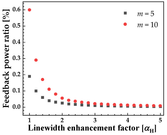
Figure 7.
Hopf bifurcation point vs. linewidth enhancement factor under I = 1.1Ith, τf = 2.4 ns.
For ICLs, the number of stages, m, is usually less than 20. Figure 8 shows the Hopf bifurcation point value versus stage number with I = 1.5Ith, τf = 2.4 ns. It is seen that an increased stage number gives rise to an exponential increasing Hopf bifurcation point value, which indicates that ICLs with a large number of stages are more stable.
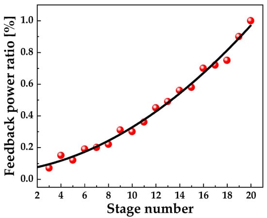
Figure 8.
Hopf bifurcation point value vs. stage number m with I = 1.5Ith, τf = 2.4 ns.
3.3. Bandwidth of Chaos
A broadband RF spectrum is one of the significant characteristics of chaos. The bandwidth of chaos determines the range resolution of chaotic lidar [37], the bit rate of random sequence generation [38] and the transmission rate of optical chaos communications [39]. We use a conventional definition of bandwidth of chaotic signals as the frequency span between the DC and the frequency where 80% of the energy is contained [40], and investigate the bandwidth of mid-infrared chaos. Similar to regular quantum well laser diodes, the bandwidth of chaos from ICL with external optical feedback increases as the feedback power ratio increases, as shown in Figure 9.
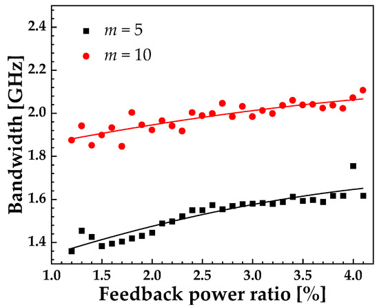
Figure 9.
Bandwidth of chaos vs. feedback power ratio under I = 1.1Ith, τf = 2.4 ns, m = 5 (black squares) and m = 10 (red circles).
Increasing the pump current and hence the relaxation oscillation frequency is expected to enhance the bandwidth of chaos, and this is confirmed in Figure 10. Here, we notice that mid-infrared chaos from ICL with different stage numbers has the same increasing tendency. Once the pump current increases to 2Ith, a 6 GHz chaos bandwidth is obtained when the stage number is 10, and a 8 GHz chaos bandwidth can be achieved with 3Ith, as shown in Figure 10.
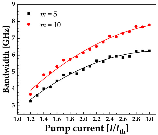
Figure 10.
Bandwidth of chaos vs. bias current when fext = 28% and τf = 2.4 ns with m = 5 (black squares), m = 10 (red circles).
Figure 11 respectively presents the time series, auto-correlation, phase diagram, RF spectrum and optical spectral of mid-infrared chaos for m = 5 (in Figure 11a) and m = 10 (in Figure 11b). This indicates that for relatively high number of stages the bandwidth of chaos from ICLs is further enhanced, as shown in Figure 11(a-iv,b-iv). The enhanced bandwidth of the chaos is due to the relaxation oscillation frequency of the ICL increasing with the number of stages.
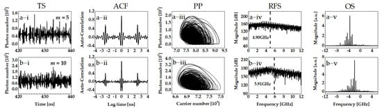
Figure 11.
Output chaos of ICL with external optical feedback as stage number increases with I = 1.9Ith, τf = 2.4 ns and fext = 28%. (a) m = 5, (b) m = 10. Columns (i–v) are TS, ACF, PP, RFS, OS, respectively.
The stage number effect is presented in Figure 12, where m ranges from 3 to 20 and the pump currents are 1.1Ith (black squares) and 2Ith (red circles). Although the increase in bandwidth for the relatively high pump current, 2Ith, is faster than that of the relatively low pump current, 1.1Ith, the tendency of the stage number effects is the same, that is the bandwidth of chaos increases as the stage number increases. This tendency is verified in Figure 9, Figure 10 and Figure 11.
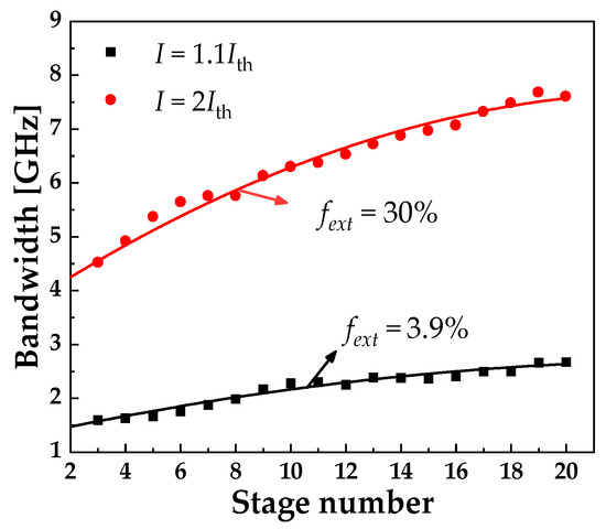
Figure 12.
Bandwidth of chaos vs. stage number I = 1.1Ith (black squares) and I = 2Ith (red circles) with τf = 2.4 ns.
By using Maximum Lyapunov exponents, we distinguish chaos from QP, and calculate the 80% energy power bandwidth versus feedback power ratio and pump current, as shown in Figure 13. By using dashed curves, we distinguish QP and C, while the white region represents the stable(S) output. It is found, in Figure 13a, that S is observed for a small number of stages m = 5 when the bias current is below 1.2Ith and the feedback power ratio is in the range of 4% to 30%. Stable output is also found in the top left corner of Figure 13a. For a large stage number, that is m = 10, S is observed when the pump current is small, below 1.2Ith, and the feedback power ratio is around 28%, as indicated in the bottom right corner of Figure 13b. S is also observed for m = 10 when the bias current is higher than 2.16Ith and the feedback power ratio is less than 4%, as seen in Figure 13b. These results indicate that an ICL with a relatively high bias current will exhibit S, QP and then enter into C as the feedback power ratio increases. As the stage number increases from 5 to 10 and the ICL is subject to a relatively high bias current, both S and QP regions are extended, as shown towards the left of Figure 13a,b. This confirms that for relatively few stage numbers an ICL with external optical feedback is amenable to exhibiting chaos. The results for both cases confirm that in order to obtain broadband mid-infrared chaos, one needs a relatively high pump current as well as a large feedback power ratio. Furthermore, a 8 GHz bandwidth of mid-infrared chaos can be obtained for m = 10, as shown in the top right corner of Figure 13b.
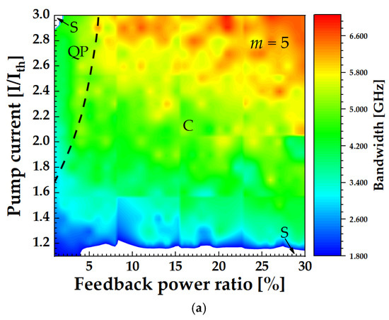
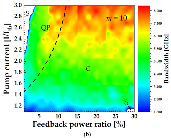
Figure 13.
Bandwidth vs. feedback power ratio and pump current, with τf = 2.4 ns. (a) m = 5, (b) m = 10.
4. Discussion
A mid-infrared chaotic laser will be a promising source for implementing secure free-space optical communication. In this paper, we show how to obtain broadband mid-infrared chaos using an ICL with long-cavity optical feedback. The analysis of the laser stability is effected by identifying the Hopf bifurcation point. From such considerations we find that ICLs with a relatively small number of stages are more unstable and thus susceptible to exhibiting chaos. The chaos bandwidth of the ICL is related to the relaxation oscillation frequency, which increases linearly with the cube root of the stage number and laser pump current. Therefore, to obtain broadband chaos from an ICL there is a need for a high pump current, large number of stages as well as strong optical feedback strength. Our calculations show that 8 GHz bandwidth mid-infrared chaos can be generated using a 10-stage ICL biased at three times the threshold current. With the availability of such broadband mid-infrared chaos, it is expected that of-order Gbit/s secure free-space optical communication is feasible.
Author Contributions
Conceptualization, H.H. and K.A.S.; software, X.C.; formal analysis and validation, H.H. and K.A.S.; investigation, K.A.S.; resources, H.H.; data curation, X.C.; writing—original draft preparation, H.H.; writing—review and editing, K.A.S.; visualization, X.C.; supervision, H.H. and Z.J.; project administration, H.H.; funding acquisition, H.H. and Z.J. All authors have read and agreed to the published version of the manuscript.
Funding
This research was funded by National Natural Science Foundation of China grant number 61805168 and 61741512, Research Project Supported by Shanxi Scholarship Council of China grant number 2021032, Shanxi “1331 Project” Key Innovative Team; Program for Top Young and Middle-aged Innovative Talents of Shanxi, and Key Research and Development Project grant number 201903D121124.
Institutional Review Board Statement
Not applicable.
Informed Consent Statement
Not applicable.
Data Availability Statement
The data presented in this study are available on request from the corresponding author.
Conflicts of Interest
The authors declare no conflict of interest. The funders had no role in the design of the study; in the collection, analyses, or interpretation of data; in the writing of the manuscript, or in the decision to publish the results.
Abbreviations
The following abbreviations are used in this manuscript:
| ICL | interband cascade laser |
| LEF | linewidth enhancement factor |
| QCL | quantum cascade laser |
| TS | time series |
| ACF | autocorrelation curves functions |
| PP | phase portrait |
| RFS | radio-frequency spectrum |
| OS | optical spectral |
| S | stable |
| P1 | period-1 |
| QP | quasi-periodic |
| MP | multiple-periodic |
| C | chaos |
References
- Lin, C.-H.; Yang, R.Q.; Zhang, D.; Murry, S.; Pei, S.; Allerman, A.; Kurtz, S. Type-II interband quantum cascade laser at 3.8 μm. Electron. Lett. Abbrevi. 1997, 33, 598–599. [Google Scholar] [CrossRef]
- Yang, R.Q.; Bradshaw, J.L.; Bruno, J.D. Room temperature type-II interband cascade. Appl. Phys. Lett. 2002, 81, 397–399. [Google Scholar] [CrossRef]
- Yang, R.Q.; Hill, C.J.; Yang, B.H.; Wong, C.M.; Muller, R.E.; Echternach, P.M. Continuous-wave operation of distributed feedback interband cascade lasers. Appl. Phys. Lett. 2004, 84, 3699–3701. [Google Scholar] [CrossRef]
- Kim, M.; Canedy, C.L.; Bewley, W.W.; Kim, C.S.; Lindle, J.R.; Abell, J.; Vurgaftman, I.; Meyer, J.R. Interband cascade laser emitting at λ = 3.75 μm in continuous wave above room temperature. Appl. Phys. Lett. 2008, 92, 191110. [Google Scholar] [CrossRef]
- Bagheri, M.; Frez, C.; Sterczewski, L.; Gruidin, I.; Fradet, M.; Vurgaftman, I.; Canedy, C.L.; Bewley, W.W.; Merritt, C.D.; Kim, C.S.; et al. Passively mode-locked interband cascade optical frequency combs. Sci. Rep. 2018, 8, 3322. [Google Scholar] [CrossRef] [PubMed] [Green Version]
- Yang, H.; Yang, R.Q.; Gong, J.; He, J.-J. Mid-Infrared Widely Tunable Single-Mode Interband Cascade Lasers Based on V-Coupled Cavities. Opt. Lett. 2020, 45, 2700–2702. [Google Scholar] [CrossRef] [PubMed]
- Chen, C.C. Attenuation of Electromagnetic Radiation by Haze, Fog, Clouds, and Rain; Rand Corp.: Santa Monica, CA, USA, 1975; pp. 1–39. [Google Scholar]
- Vurgaftman, I.; Weih, R.; Kamp, M.; Meyer, J.R.; Canedy, C.L.; Kim, C.S.; Kim, M.; Bewley, W.W.; Merritt, C.D.; Abell, J.; et al. Interband cascade lasers. J. Phys. D Appl. Phys. 2005, 48, 123001. [Google Scholar] [CrossRef]
- Horstjann, M.; Bakhirkin, Y.; Kosterev, A.; Curl, R.; Tittel, F.; Wong, C.; Hill, C.; Yang, R. Formaldehyde sensor using interband cascade laser based quartz-enhanced photoacoustic spectroscopy. Appl. Phys. B 2004, 79, 799–803. [Google Scholar] [CrossRef]
- Wysocki, G.; Bakhirkin, Y.; So, S.; Tittel, F.K.; Hill, C.J.; Yang, R.Q.; Fraser, M.P. Dual interband cascade laser based trace-gas sensor for environmental monitoring. Appl. Opt. 2007, 46, 8202–8209. [Google Scholar] [CrossRef] [Green Version]
- Risby, T.H.; Tittel, F.K. Current status of midinfrared quantum and interband cascade lasers for clinical breath analysis. Opt. Eng. 2010, 49, 111123. [Google Scholar]
- Soibel, A.; Wright, M.W.; Farr, W.H.; Keo, S.A.; Hill, C.J.; Yang, R.Q.; Liu, H.C. Midinfrared Interband Cascade Laser for Free Space Optical Communication. IEEE Photonics Technol. Lett. 2010, 22, 121–123. [Google Scholar] [CrossRef]
- Yang, R.Q.; Li, L.; Jiang, Y.C. Interband cascade laser: From original concept to actual device. Prog. Phys. 2014, 34, 169–190. [Google Scholar]
- Deng, Y.; Zhao, B.B.; Wang, C. Linewidth broadening factor of an interband cascade laser. Appl. Phys. Lett. 2019, 115, 181101. [Google Scholar] [CrossRef]
- Green, R.P.; Xu, J.-H.; Mahler, L.; Tredicucci, A.; Beltram, F.; Giuliani, G.; Beere, H.E.; Ritchie, D. Linewidth enhancement factor of terahertz quantum cascade lasers. Appl. Phys. Lett. 2008, 92, 071106. [Google Scholar] [CrossRef] [Green Version]
- Deng, Y.; Fan, Z.F.; Wang, C. Optical feedback induced nonlinear dynamics in an interband cascade laser. Proc. SPIE 2021, 11680, 116800J. [Google Scholar]
- Spitz, O.; Herdt, A.; Wu, J.; Maisons, G.; Carras, M.; Wong, C.-W.; Elsäßer, W.; Grillot, F. Private communication with quantum cascade laser photonic chaos. Nat. Commun. 2021, 12, 3327. [Google Scholar] [CrossRef]
- Caffey, D.; Day, T.; Kim, C.S.; Kim, M.; Vurgaftman, I.; Bewley, W.W.; Lindle, J.R.; Canedy, C.L.; Abell, J.; Meyer, J.R. Performance characteristics of a continuous wave compact widely tunable external cavity interband cascade lasers. Opt. Express 2010, 18, 15691. [Google Scholar] [CrossRef]
- Wang, A.; Li, P.; Zhang, J.; Zhang, J.; Li, L.; Wang, Y. 4.5 Gbps high-speed real-time physical random bit generator. Opt. Express 2013, 21, 20452–20462. [Google Scholar] [CrossRef]
- Wang, A.; Yang, Y.; Wang, B.; Zhang, B.; Li, L.; Wang, Y. Generation of wideband chaos with suppressed time-delay signature by delayed self-interference. Opt. Express 2013, 21, 8701–8710. [Google Scholar] [CrossRef] [PubMed]
- Wang, L.; Wang, D.; Gao, H.; Guo, Y.; Wang, Y.; Hong, Y.; Shore, K.A.; Wang, A. Real-time 2.5-Gb/s correlated random bit generation using synchronized chaos induced by a common laser with dispersive feedback. IEEE J. Quantum Electron. 2020, 56, 1–8. [Google Scholar] [CrossRef]
- Zhang, T.; Jia, Z.; Wang, A.; Hong, Y.; Wang, L.; Guo, Y.; Wang, Y. Experimental observation of dynamic-state switching in VCSELs with optical feedback. IEEE Photonics Technol. Lett. 2021, 33, 335–338. [Google Scholar] [CrossRef]
- Jumpertz, L.; Schires, K.; Carras, M.; Sciamanna, M.; Grillot, F. Chaotic light at mid-infrared wavelength. Light Sci. Appl. 2016, 5, e16088. [Google Scholar] [CrossRef] [Green Version]
- Spitz, O.; Wu, J.; Carras, M.; Wong, C.-W.; Grillot, F. Low-frequency fluctuations of a mid-infrared quantum cascade laser operating at cryogenic temperatures. Laser Phys. Lett. 2018, 15, 116201. [Google Scholar] [CrossRef] [Green Version]
- Jumpertz, L.; Carras, M.; Grillot, F. Regimes of external optical feedback in 5.6 µm distributed feedback mid-infrared quantum cascade lasers. Appl. Phys. Lett. 2014, 105, 131112. [Google Scholar] [CrossRef] [Green Version]
- Panajotov, K.; Sciamanna, M.; Arteaga, M.A.; Thienpont, H. Optical feedback in vertical-cavity surface-emitting lasers. IEEE J. Sel. Top. Quantum Electron. 2013, 19, 1700312. [Google Scholar] [CrossRef]
- Yang, R.Q. Mid-infrared interband cascade lasers based on type-II heterostructures. Microelectron. J. 1999, 30, 1043–1056. [Google Scholar] [CrossRef]
- Lang, R.; Kobayashi, K. External optical feedback effects on semiconductor injection laser properties. IEEE J. Quantum Electron. 1980, 16, 347–355. [Google Scholar] [CrossRef]
- Deng, Y.; Wang, C. Rate Equation modeling of interband cascade lasers on modulation and noise dynamics. IEEE J. Quantum Electron. 2020, 56, 2300109. [Google Scholar] [CrossRef]
- Bewley, W.W.; Lindle, J.R.; Kim, C.S.; Kim, M.; Canedy, C.L.; Vurgaftman, I.; Meyer, J.R. Lifetimes and Auger coefficients in type-II W interband cascade lasers. Appl. Phys. Lett. 2008, 93, 041118. [Google Scholar] [CrossRef]
- Vurgaftman, I.; Canedy, C.L.; Kim, C.S.; Kim, M.; Bewley, W.W.; Lindle, J.R.; Abell, J.; Meyer, J.R. Mid-infrared interband cascade lasers operating at ambient temperatures. New J. Phys. 2009, 11, 125015. [Google Scholar] [CrossRef] [Green Version]
- Vurgaftman, I.; Canedy, C.L.; Kim, C.S.; Kim, M.; Bewley, W.W.; Lindle, J.R.; Abell, J.; Meyer, J.R. Mid-IR type-II interband cascade lasers. IEEE J. Sel. Top. Quantum Electron. 2011, 17, 1435–1444. [Google Scholar] [CrossRef]
- Wolf, A.; Swift, J.B.; Swinney, H.L.; Vastano, J.A. Determining Lyapunov exponents from a time-series. Phys. D Nonlinear Phenomena. 1985, 16, 285–317. [Google Scholar] [CrossRef] [Green Version]
- Wolf, A. Wolf Lyapunov Exponent Estimation from A Time Series. MATLAB Central File Exchange. Available online: https://www.mathworks.com/matlabcentral/fileexchange/48084-wolf-lyapunov-exponent-estimation-from-a-time-series (accessed on 5 January 2021).
- Wang, D.; Wang, L.; Li, P.; Zhao, T.; Jia, Z.; Gao, Z.; Guo, Y.; Wang, Y.; Wang, A. Bias Current of Semiconductor Laser-An Unsafe Key for Secure Chaos Communication. Photonics 2019, 6, 59. [Google Scholar] [CrossRef] [Green Version]
- Huang, Y.; Zhou, P.; Li, N.Q. Broad tunable photonic microwave generation in an optically pumped spin-VCSEL with optical feedback stabilization. Opt. Lett. 2021, 46, 3147–3150. [Google Scholar] [CrossRef]
- Wang, B.; Wang, Y.; Kong, L.; Wang, A. Multi-target real-time ranging with chaotic laser radar. Chin. Opt. Lett. 2008, 6, 868–870. [Google Scholar] [CrossRef]
- Li, P.; Guo, Y.; Guo, Y.; Fan, Y.; Guo, X.; Liu, X.; Shore, K.A.; Dubrova, E.; Xu, B.; Wang, Y.; et al. Self-balanced real-time photonic scheme for ultrafast random number generation. APL Photonics 2018, 3, 061301. [Google Scholar] [CrossRef]
- Wang, L.; Mao, X.; Wang, A.; Wang, Y.; Gao, Z.; Li, S.-S.; Yan, L. Scheme of coherent optical chaos communication. Opt. Lett. 2020, 45, 4762. [Google Scholar] [CrossRef]
- Lin, F.Y.; Liu, J.M. Nonlinear dynamical characteristics of an optically injected semiconductor laser subject to optoelectronic feedback. Opt. Commun. 2003, 221, 173–180. [Google Scholar] [CrossRef]
Publisher’s Note: MDPI stays neutral with regard to jurisdictional claims in published maps and institutional affiliations. |
© 2021 by the authors. Licensee MDPI, Basel, Switzerland. This article is an open access article distributed under the terms and conditions of the Creative Commons Attribution (CC BY) license (https://creativecommons.org/licenses/by/4.0/).