Abstract
The statistics of the optical phase of the light emitted by a semiconductor laser diode when subject to periodic modulation of the applied bias current are theoretically analyzed. Numerical simulations of the stochastic rate equations describing the previous system are performed to describe the temporal dependence of the phase statistics. These simulations are performed by considering two cases corresponding to random and deterministic initial conditions. In contrast to the Gaussian character of the phase that has been assumed in previous works, we show that the phase is not distributed as a Gaussian during the initial stages of evolution. We characterize the time it takes the phase to become Gaussian by calculating the dynamical evolution of the kurtosis coefficient of the phase. We show that, under the typical gain-switching with square-wave modulation used for quantum random number generation, quantity is in the ns time scale; that corresponds to the time it takes the system to lose the memory of the distribution of the initial conditions. We compare the standard deviation of the phase obtained with random and deterministic initial conditions to show that their differences become more important as the modulation speed is increased.
1. Introduction
Experimental and theoretical understanding of the fluctuations of laser light began shortly after the invention of the laser [1,2,3,4,5]. Special attention has been devoted to fluctuations of the light emitted by semiconductor lasers [6,7,8,9,10] due to their vast variety of applications. The best available theoretical description of these fluctuations is based on the Fokker–Planck equation, or alternativelly on Langevin’s stochastic rate equations [3,6,7,8,11]. The phase of the laser electrical field is a random quantity, mainly due to the effect of the spontaneous emission noise. The random character of this phase is precisely the basis of some of the available methods for quantum random number generation (QRNG).
Random numbers are a vital resource for numerous applications including cryptography, statistical analysis, stochastic simulations, decission making in engineering processes, quantitative finance, gambling, massive data processing, etc. [12,13]. Random number generators (RNG) use software algorithms (pseudorandom number generators) or hardware physical devices. Typical physical processes used to generate random numbers are radioactive decay, Johnson or Zener’s noise, chaos noise [13,14] and quantum phenomena [12,13]. QRNGs are a particular case of physical RNGs that can generate truly random numbers from the fundamentally probabilistic nature of quantum events [13]. The advantage of using QRNGs relies on its unpredictibility, which can be proven to be based on quantum physics laws. Typical QRNGs are based on quantum optics [13]. These generators can be divided in (i) generators that use single-photon sources, and (ii) generators that use multi-photon sources, typically semiconductor lasers or LEDs. QRNGs based on single-photon detection methods include: Branching path generators [15], generators measuring the time of arrival of photons [16], photon counting generators [17], and attenuated pulse generators [18]. These methods have been experimentally compared in [19]. Multi-photon QRNGs include: Generators based on quantum vacuum fluctuations [20], on amplified spontaneous emission (ASE) signals [21,22], and on phase noise in continuous wave [23,24,25] and in pulsed laser diodes [26,27,28,29,30,31].
Spontaneous emission is a useful mechanism to generate quantum fluctuations, as it can be ascribed to the vacuum fluctuations of the optical field [26]. Randomness due to spontaneous emission is the basis of QRNGs based on pulsed single-mode laser diodes [26,27,28,30,31]. These generators have several advantages. They are made of commercially available components: For instance, standard photodetectors can be used due to the high signal levels. They are simple, low-cost, robust, and fast: Generation rates up to 43 Gbps quantum random bit generation have been experimentally demonstrated [27]. In these QRNGs the laser diode is periodically modulated from below to above threshold in such a way that gain-switching operation is obtained, typically at Gbps rates. While the laser is below threshold the optical phase becomes random due to the spontaneous emission noise. Gain-switching operation produces a periodic train of laser pulses with random phases. Phase fluctuations are then converted into amplitude fluctuations by using interferometric setups [27,31]. Detection and filtering of the amplitude fluctuations provides the generation of random values with an almost uniform distribution.
The applications of QRNGs, for instance in cryptography [31,32], require that the physical processes underlying their operation must be properly understood and described. For QRNGs based on pulsed semiconductor lasers, it is essential an accurate description of the phase diffusion process, that is, laser phase fluctuations must be qualitatively and quantitatively characterized. Modelling of these fluctuations has been performed by numerical integration of the laser stochastic rate equations [27,30,31,33,34,35,36]. Good quantitative agreement between experiments and theory is achieved when the complete set of parameters of the rate equations is known for the specific laser diode. Good agreement between experimental and theoretical phase fluctuations has been recently reported for a discrete mode laser (DML) [36] for which a complete extraction of the intrinsic parameters was performed [35,37]. This permits a quantitative description of the dependence of phase diffusion on the laser and modulation parameters. On the qualitative side, statistics of optical phase has been described as Gaussian in numerical simulations [27,33,34] since spontaneous emission noise has also Gaussian distribution. However, in these generators the bias current is periodically modulated in such a way that the evolution is mainly in a transient regime, specially when operating at fast bit rates. It is then expected that the choice of initial conditions in the simulations must have impact on the statistics of the optical phase and on the time it takes the phase to be distributed as a Gaussian. This is in fact the main objective of this work: The investigation of the conditions for which the phase becomes distributed as a Gaussian.
In this paper we report a theoretical study of the phase diffusion in gain-switched semiconductor lasers. This is done by performing numerical simulations of the stochastic rate equations for the complex electrical field and carrier number. In our modelling we use the set of parameters recently extracted for a DML device. With these parameters we first analyze the impact of the carrier noise on the phase statistics. In the rest of the paper we focus on the calculation of the temporal dependence of the statistical moments and distribution of the phase. We first consider random initial conditions that contrast to previous analysis in which deterministic fixed initial conditions were chosen [34]. We compare the phase statistics obtained for both types of initial conditions. For both cases we show that the phase is not distributed as a Gaussian because of the non-Gaussianity of the initial conditions. This contrasts to the Gaussian character of the phase that has been assumed in previous works [27,33,34]. We characterize the time it takes the phase becomes approximately Gaussian by calculating the temporal evolution of the kurtosis coefficient of the phase. Our calculations indicate that under the typical gain-switching with square-wave modulation used for QRNG, the time it takes to the phase to become Gaussian is in the ns scale. These are the typical times for which the memory of the distribution of the initial conditions is lost. The comparison between the variance of the phase obtained with random and fixed initial conditions show that their differences become more important as the modulation speed is increased.
2. Theoretical Model
Gain-switched single-mode semiconductor laser dynamics can be modelled by using a set of stochastic rate-equations that read (in Ito’s sense) [6,37,38]
where is the number of photons inside the laser, is the optical phase, and is the number of carriers in the active region. The parameters appearing in these equations are the following: is the differential gain, is the number of carriers at transparency, is the non-linear gain coefficient, is the photon lifetime, is the linewidth enhancement factor, e is the electron charge, and and C are the non-radiative, spontaneous, and Auger recombination coefficients, respectively. In these equations we consider a temporal dependence of the injected current, , and a rate of the spontaneous emission given by where is the fraction of spontaneous emission coupled into the lasing mode. The Langevin terms and in Equations (1) and (2), represent fluctuations due to spontaneous emission, with the following correlation properties, , where is the Dirac delta function and the Kronecker delta function with the subindexes i and j referring to the variables P and .
QRNG systems based on gain-switching of single-mode laser diodes are such that a large signal modulation of the bias current is applied to the device. We consider an injected current following a square-wave modulation of period T with during , and during the rest of the period. This modulation is such that , where is the threshold current of the laser, for obtaining a random evolution of the optical phase induced by the spontaneous emission noise. Numerical integration of the previous stochastic rate equations by usual Euler–Maruyama [3,39] or Heun’s predictor-corrector algorithms [37] present instabilities when the photon number is very small, a situation always present in this type of QRNGs: some spontaneous noise events cause negative values of P that lead to numerical instabilities due to the square root factor multipliying the noise term in Equations (1) and (2). Very recently a set of rate equations for the complex electrical field, , instead of equations for P and has been proposed to solve this problem [35]. These equations are the following:
where is the complex electrical field and is the complex Gaussian white noise with zero average and correlation given by that represents the spontaneous emission noise, and where we have considered that . These equations exactly correspond to our initial model because the application of the rules for the change of variables in the Ito’s calculus [11] to and in Equations (4) and (5) gives Equations (1)–(3). Instabilities do not appear because P is not inside the square root factor that multiplies the noise term.
Up to now we have considered an equation for N that has not any noise term. Carrier noise can also be important for describing statistics in semiconductor laser dynamics [6]. These fluctuations can be taken into account if we substitute Equation (5) by
where is a real Gaussian white noise of zero average and correlation given by and statistically independent of [6,10,37,40].
In this work we will numerically solve Equations (4) and (6) by using the Euler–Maruyama algorithm [3,39] with an integration time step of 0.001 ps. We will use the numerical values of the parameters that have been extracted for a discrete mode laser (DML) [35,37]. This device is a single longitudinal mode semiconductor laser emitting close to 1550 nm wavelength and mA at a temperature of 25 C. The values of the parameters are s, , , ps, , , s, s, and s [35,37]. Simulation and experimental results have shown not only qualitative but also a remarkable quantitative agreement for a very wide range of gain-switching conditions [35,37,41].
3. Analysis of the Dynamics
We first analyze the dynamical evolution of relevant variables when the laser is modulated with mA, = 7 mA, and ns. The laser is switched-off with a current close to , for obtaining a significant effect of the spontaneous emission noise on the randomness of the phase. Figure 1a–c show the photon number, carrier number, and optical phase, respectively, as a function of time. We integrate the equations for consecutive bias current pulses in such a way that the initial conditions for one period correspond to the final values of the variables at the end of the previous period. Figure 1a shows P for three consecutive pulses. The laser is switched-on with at ns. After this time P begins to build-up from very small random values determined by the spontaneous emission noise events. After the emission of the pulse with the corresponding relaxation oscillations, P begins to decrease at ns (when is applied), reaching the small random values at which spontaneous emission noise dominates the device dynamics. N begins at ns from a value well below the threshold carrier number, , as it can be seen in Figure 1b. The characteristics relaxation oscillations of N associated to the pulse emission are followed by a monotonous decrease from ns to 2 ns due to the value below threshold of .
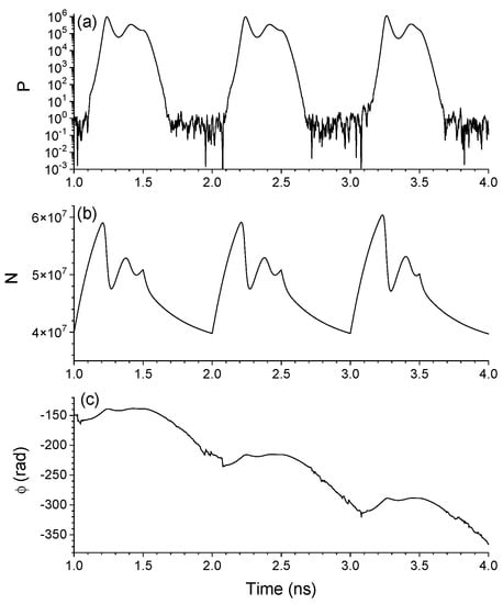
Figure 1.
(a) Photon number, (b) carrier number, and (c) optical phase as a function of time for three consecutive pulses when 1 ns.
The optical phase is calculated at each integration step from and in such a way that it is a continuous function of t. The dynamical evolution of is shown in Figure 1c. When P is large (small) the noise term in Equation (2) is much smaller (larger) than the other term in that equation and mainly evolves in a deterministic (random) way. The deterministic decrease of is due to the value below threshold of the current when switching-off the laser: because , and therefore decreases (see Equation (2)).
Visualization of different random trajectories and calculation of statistical moments of the phase, specially its standard deviation, , have been usually done by overlaying them in a temporal window with a duration of a few periods [33,34,35]. For instance just one period is considered in references [34,35] to calculate the value of with . To obtain well defined averages, and , it is necessary to make a choice of the initial conditions at the beginning of each period because is an unbounded quantity, as shown in Figure 1. One choice is to take , , and [34], that is fixed initial conditions. A second choice is to take random initial conditions [35]. Photon and carrier numbers at are those obtained at the end of the previous period, like in Figure 1. The change with respect to Figure 1 is related to the phase and it is based on the cyclic nature of angles: We consider that at the beginning of the period, , is that corresponding to at the end of the previous period, , but converted into the range, that is we consider that is given by .
Figure 2 shows the temporal evolution of P, N and , plotted in a window of duration T, corresponding to the three consecutive pulses of Figure 1 and using the previous choice of random initial conditions. Figure 2a,c show that laser pulses that have a larger switch-on time, defined as the time at which P crosses a fixed level, have also a larger value of the maximum of N and P [9]. Figure 2b shows that takes values in a range of several multiples of 2 during one period. Figure 2b also shows, in a more clear way than in Figure 1, that the phase fluctuations are more important at the beginning and at the end of the pulse. Comparison between Figure 2a,b shows that pulses with a similar evolution of P can have a very different phase evolution (see black and red realizations). In the next section we will focus on the description of the temporal evolution of the phase statistics.
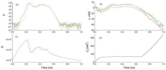
Figure 2.
(a) Photon number, (b) phase, and (c) carrier number dynamical evolution for three different realizations are shown with black, red, and green lines in a temporal window of duration T. (d) Variance of the phase as a function of t. In this figure 1 ns and the three realizations are extracted from the time traces of Figure 1.
4. Analysis of the Phase Statistics
The dynamical evolution of the variance of the phase, , is shown in Figure 2d for the case of random initial conditions and a temporal window of duration 1 ns. has been calculated by averaging over 2 × 10 temporal windows. because of our choice of random initial conditions. Large increases of occur while P is small and dominated by the spontaneous emission noise, that is at the beginning and at the end of the period. While the evolutions of P and are deterministic and (0.15 ns < t < 0.5 ns) oscillates with the frequency of the relaxation oscillations around a value that increases linearly with time, similarly to what was observed by Henry [8]. These oscillations and the linear increase are barely seen in Figure 2d because of the vertical scale determined by the large values of the variance when the laser is switched-off. From 0.5 ns < t < 0.65 ns, while still has a deterministic evolution, there is a slight decrease of . After that time, both and P become determined by the spontaneous emission noise. In this way the linear increase of with t, characteristic of phase diffusion, is observed until the end of the period, as it is seen in Figure 2d.
We now analyze the effect of carrier noise on the statistics of the phase. Figure 3 shows the probability density function (pdf) of at three different times when the carrier noise is considered (that is, integrating Equation (6)) and when it is neglected (considering instead Equation (5)). This figure has been obtained using the same conditions of Figure 2.
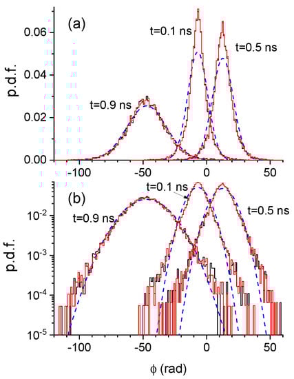
Figure 3.
Probability density function of the phase at three different times in (a) linear, and (b) logarithmic vertical scale. Pdfs obtained with and without noise in the carrier number equation are plotted with red and black solid lines. Gaussian approximations are plotted with blue dashed lines.
Figure 3 shows that the effect of carrier noise on the statistics of is very small. In fact, it has been shown that the consideration of noise in the carrier equation is not important during transient regimes [9,33], being only essential in the stationary regime for calculating quantities like the relative intensity noise [6]. Figure 3 also shows the Gaussian distributions of average and standard deviation given by the simulation with carrier noise. It is clear that the Gaussian distribution does not describe well the phase satististics, specially for short times ( and ns). The Gaussian approximation becomes better at longer times ( ns).
A way of quantifying if the Gaussian distribution is suitable for describing the phase statistics is by calculating moments of of order higher than 2. Asymmetry and kurtosis coefficient of the simulated data are shown in Figure 4 as a function of time. Both coefficients must vanish if the distribution is Gaussian. Figure 4a shows with black lines the asymmetry, , and kurtosis, , coefficients obtained under the same conditions of Figure 2, that is with random initial conditions. While the phase distribution is symmetric (), is significantly larger than zero. decreases fast until it develops a small peak close to the time at which the first relaxation oscillation appears. After that peak it reaches a plateau that finishes when P reaches the spontaneous emission noise level (around 0.7 ns). From that time diffuses and monotonously decreases reaching values that are closer to zero at the end of the period ( 0.65 at ns). Figure 4b shows and when 2 ns. In this case has more time to diffuse when the laser is switched-off and then the Gaussian approximation is better at the end of the period ( 0.14 at ns).
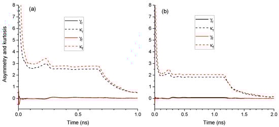
Figure 4.
Asymmetry and kurtosis coefficients of the phase as a function of time for (a) T = 1 ns, and (b) T = 2 ns. Asymmetry and kurtosis coefficients are plotted with solid and dashed lines, respectively. Results for random and fixed initial conditions are plotted with black and red lines, respectively.
The reason why is not Gaussian can be understood by plotting the pdf of at . Figure 5 shows that distribution for the case of ns. The distribution corresponds to a uniform random variable in . This is because of the way random initial conditions are chosen: Doing the operation from a broad nearly Gaussian distribution for makes a uniform random variable, U. The kurtosis of U is . Diffusion of at the beginning of the period (see Figure 2) makes to decrease quickly, but not enough for becoming strictly Gaussian, even at the end of the period.
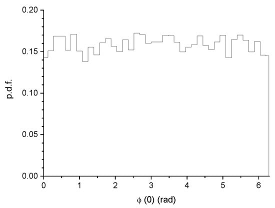
Figure 5.
Probability density function of the initial value of the phase for T = 1 ns.
Of course these results depend on the way initial conditions are chosen. Another way of choosing these values is by considering fixed initial values for and . Figure 4 shows, with red lines, asymmetry and kurtosis coefficients, and , when fixed initial conditions are used. We choose these values in the following way. We first integrate Equations (4) and (6) from arbitrary initial conditions corresponding to below threshold operation in order to find the averaged and for . Then we choose and . This election is similar to that considered in [34]. Figure 4 shows that the evolution of and is very similar to that of and , respectively. because the initial delta-like distribution of produce larger values of the kurtosis. These differences decrease with t, specially when spontaneous emission dominates the phase evolution: In Figure 4a,b when ns ( ns).
The choice of initial conditions also impacts on the values of the standard deviation as a function of t. In Figure 6a the dynamical evolution of for both, random and fixed initial conditions, is shown when ns. Again both standard deviations have similar trends but the value for random initial conditions is larger than that obtained for the fixed ones. This is due to the non-zero value of obtained with the uniform distribution of in contrast to the zero value obtained for fixed initial conditions. Relative differences between both quantities enhance if the speed of QRNG increases as it can be seen in Figure 6b where results obtained for ns have been plotted. For instance, at 0.2 ns is around 20 % smaller for the case of fixed initial conditions.
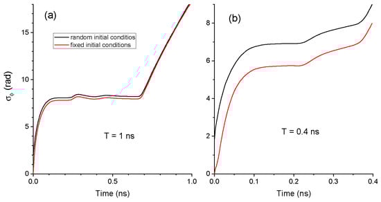
Figure 6.
Standard deviation of the phase as a function of time for (a) T = 1 ns, and (b) T = 0.4 ns. Results for random and fixed initial conditions are plotted with black and red lines, respectively.
The dependence of the phase statistics on the way initial conditions are chosen suggests that averages must be done in a different way in order to lose the memory of those initial conditions. We have been considering averages performed in a temporal window with the same duration than the period of the current, T. From now on we will consider longer temporal windows for calculating statistical averages. Figure 7 illustrates the situation found when averages are calculated over a window of duration 2T. Random initial conditions are considered such that . Averages have been done over 2 × 10 2T-windows, where T = 1 ns, in order to compare with situations illustrated in previous figures. Figure 7a shows the averaged phase vs. t. The drift towards decreasing values of the phase is similar to that shown in Figure 1c. Standard deviation and variance of the phase are shown in Figure 7b,c, respectively. , and during the second half of the -window are basically replicas of what was found in the first half. The continuity of along the 2T-window makes that and monotonously increase. However the situation is different when considering the kurtosis coefficient as Figure 7d shows. In this case, during the second half of the window keeps on decreasing towards the zero value. This means that the distribution of the phase keeps on approaching to the Gaussian shape. In fact = 0.22 when t = 2 ns.
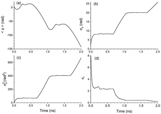
Figure 7.
(a) Average, (b) standard deviation, (c) variance, and (d) kurtosis coefficient of the phase as a function of time for a two-period window with T = 1 ns.
That approach can be illustrated by plotting the phase pdf at two different times. Figure 8 shows those distributions at times and ns. The phase at is a U random variable, similarly to Figure 5. The phase at ns is approximately Gaussian as it can be seen when comparing with the Gaussian of average and standard deviation obtained from simulations. The kurtosis coefficient in Figure 8b is 0.4. Figure 8b can also be compared with the pdf obtained at t = 0.1 ns in Figure 3b because both distributions correspond to 0.1 ns after switching-on the bias current. The pdf in Figure 3b is not Gaussian while the pdf in Figure 8c is approximately Gaussian. This indicates that in order to have a phase distributed as a Gaussian it is necessary to calculate and average the phase in windows with durations of several modulation periods. In this way the memory of the initial conditions and their distribution is lost.
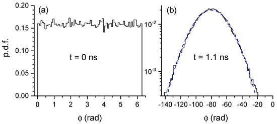
Figure 8.
Probability density function of the phase at (a) t = 0 ns, and (b) 1.1 ns for a two-period window with T = 1 ns. The Gaussian approximation is plotted with a blue dashed line.
5. Discussion and Summary
In our study we have considered two types of initial conditions, corresponding to deterministic and random values of the variables. Fixed initial conditions have been considered because they have been used in previous studies of QRNG. They are not the best choice for simulation of these systems because the spontaneous emission noise, that is always present in the system, causes fluctuations in the variables of the system at all times. These include the times at which each period begins, and so initial conditions must be also random, as it is also expected in an experimental realization of the system. We have chosen these random initial values by calculating the phase angle in the range that corresponds to the final value in the previous averaging window. Note that the conversion to the range is necessary if a calculation of well defined statistical moments of the phase is required. If no conversion is done, not even could be calculated because decreases in each averaging window in a magnitude of more than several , as illustrated for instance in Figure 1c.
Deterministic initial conditions and phase averages over windows of T-duration have been recently used for describing the phase statistics [34]. While these conditions can give an approximation to the phase distribution and their statistical moments, our results show that it is necessary to consider averages over windows of several T-duration and random initial conditions for obtaining Gaussian statistics for the phase at the end of the averaging period.
We now briefly discuss the effect of two laser parameters, the non-linear gain and the Auger coefficients, on the standard deviation of the phase. The number of relaxation oscillation peaks increases when the non-linear gain coefficient decreases. The standard deviation of the phase at the end of the modulation period oscillates when changing [35]. The number of these oscillations is directly related to the number of relaxation oscillation peaks that are excited. In this way, the main effect of having a small nonlinear gain coefficient is to observe more oscillations of the standard deviation of the phase as a function of . The effect of the Auger coefficient is also important for describing the standard deviation of the phase. In fact we have shown that the Auger term must be considered in the carrier recombination term for achieving good agreement between experiments and theory [36].
Summarizing, we have theoretically analyzed the phase diffusion in gain-switched semiconductor lasers by performing numerical simulations of the corresponding stochastic rate equations. We have focused on the calculation of the temporal dependence of the statistical moments and distribution of the phase. We have considered several types of initial conditions for the phase. By using the temporal dependence of the kurtosis coefficient we have shown that the phase pdf becomes Gaussian only after the memory of the statistical distribution of the initial conditions is lost. We show that under the typical gain-switching with square-wave modulation used in QRNGs, the time it takes for the phase to become Gaussian is in the ns scale. We finally compared the variance of the phase obtained with random and fixed initial conditions to show that their differences are more important as the modulation speed is increased. This is precisely the situation in which faster generation bit rates are achieved when using QRNGs based on gain-switched laser diodes.
Funding
This research was funded by Ministerio de Economía y Competitividad (MINECO/FEDER, UE), Spain under grant RTI2018-094118-B-C22.
Institutional Review Board Statement
Not applicable.
Informed Consent Statement
Not applicable.
Data Availability Statement
Not applicable.
Conflicts of Interest
The author declares no conflict of interest.
Abbreviations
The following abbreviations are used in this manuscript:
| QRNG | Quantum random number generation |
| DML | Discrete mode laser |
| Probability density function | |
| ASE | Amplified spontaneous emission |
| RNG | Random number generation |
| LED | Light emitting diode |
References
- Lax, M. Quantum noise. IV. Quantum theory of noise sources. Phys. Rev. 1966, 145, 110. [Google Scholar] [CrossRef]
- Lax, M.; Louisell, W. Quantum noise. XII. Density-operator treatment of field and population fluctuations. Phys. Rev. 1969, 185, 568. [Google Scholar] [CrossRef]
- Risken, H. Fokker–Planck equation. In The Fokker–Planck Equation; Springer: Berlin/Heidelberg, Germany, 1996. [Google Scholar]
- Henry, C.H.; Kazarinov, R.F. Quantum noise in photonics. Rev. Mod. Phys. 1996, 68, 801. [Google Scholar] [CrossRef]
- Arecchi, F.; Degiorgio, V.; Querzola, B. Time-dependent statistical properties of the laser radiation. Phys. Rev. Lett. 1967, 19, 1168. [Google Scholar] [CrossRef]
- Coldren, L.A.; Corzine, S.W.; Mashanovitch, M.L. Diode Lasers and Photonic Integrated Circuits; John Wiley & Sons: Hoboken, NJ, USA, 2012; Volume 218. [Google Scholar]
- Agrawal, G.P.; Dutta, N.K. Semiconductor Lasers; Springer: Berlin/Heidelberg, Germany, 2013. [Google Scholar]
- Henry, C. Phase noise in semiconductor lasers. J. Light. Technol. 1986, 4, 298–311. [Google Scholar] [CrossRef]
- Balle, S.; Colet, P.; San Miguel, M. Statistics for the transient response of single-mode semiconductor laser gain switching. Phys. Rev. A 1991, 43, 498. [Google Scholar] [CrossRef]
- Balle, S.; De Pasquale, F.; Abraham, N.; San Miguel, M. Statistics of the transient frequency modulation in the switch-on of a single-mode semiconductor laser. Phys. Rev. A 1992, 45, 1955. [Google Scholar] [CrossRef] [PubMed]
- Gardiner, C.W. Handbook of Stochastic Methods; Springer: Berlin/Heidelberg, Germany, 1985; Volume 3. [Google Scholar]
- Stipčević, M.; Koç, Ç.K. True random number generators. In Open Problems in Mathematics and Computational Science; Springer: Berlin/Heidelberg, Germany, 2014; pp. 275–315. [Google Scholar]
- Herrero-Collantes, M.; Garcia-Escartin, J.C. Quantum random number generators. Rev. Mod. Phys. 2017, 89, 015004. [Google Scholar] [CrossRef] [Green Version]
- Sciamanna, M.; Shore, K.A. Physics and applications of laser diode chaos. Nat. Photonics 2015, 9, 151–162. [Google Scholar] [CrossRef] [Green Version]
- Jennewein, T.; Achleitner, U.; Weihs, G.; Weinfurter, H.; Zeilinger, A. A fast and compact quantum random number generator. Rev. Sci. Instrum. 2000, 71, 1675–1680. [Google Scholar] [CrossRef] [Green Version]
- Stipčević, M.; Rogina, B.M. Quantum random number generator based on photonic emission in semiconductors. Rev. Sci. Instrum. 2007, 78, 045104. [Google Scholar] [CrossRef] [Green Version]
- Fürst, H.; Weier, H.; Nauerth, S.; Marangon, D.G.; Kurtsiefer, C.; Weinfurter, H. High speed optical quantum random number generation. Opt. Express 2010, 18, 13029–13037. [Google Scholar] [CrossRef] [PubMed]
- Wei, W.; Guo, H. Bias-free true random-number generator. Opt. Lett. 2009, 34, 1876–1878. [Google Scholar] [CrossRef]
- Durt, T.; Belmonte, C.; Lamoureux, L.P.; Panajotov, K.; Van den Berghe, F.; Thienpont, H. Fast quantum-optical random-number generators. Phys. Rev. A 2013, 87, 022339. [Google Scholar] [CrossRef] [Green Version]
- Shen, Y.; Tian, L.; Zou, H. Practical quantum random number generator based on measuring the shot noise of vacuum states. Phys. Rev. A 2010, 81, 063814. [Google Scholar] [CrossRef]
- Argyris, A.; Pikasis, E.; Deligiannidis, S.; Syvridis, D. Sub-Tb/s physical random bit generators based on direct detection of amplified spontaneous emission signals. J. Light. Technol. 2012, 30, 1329–1334. [Google Scholar] [CrossRef]
- Guo, Y.; Cai, Q.; Li, P.; Jia, Z.; Xu, B.; Zhang, Q.; Zhang, Y.; Zhang, R.; Gao, Z.; Shore, K.A.; et al. 40 Gb/s quantum random number generation based on optically sampled amplified spontaneous emission. APL Photonics 2021, 6, 066105. [Google Scholar] [CrossRef]
- Guo, H.; Tang, W.; Liu, Y.; Wei, W. Truly random number generation based on measurement of phase noise of a laser. Phys. Rev. E 2010, 81, 051137. [Google Scholar] [CrossRef] [Green Version]
- Qi, B.; Chi, Y.M.; Lo, H.K.; Qian, L. High-speed quantum random number generation by measuring phase noise of a single-mode laser. Opt. Lett. 2010, 35, 312–314. [Google Scholar] [CrossRef]
- Xu, F.; Qi, B.; Ma, X.; Xu, H.; Zheng, H.; Lo, H.K. Ultrafast quantum random number generation based on quantum phase fluctuations. Opt. Express 2012, 20, 12366–12377. [Google Scholar] [CrossRef] [Green Version]
- Jofre, M.; Curty, M.; Steinlechner, F.; Anzolin, G.; Torres, J.; Mitchell, M.; Pruneri, V. True random numbers from amplified quantum vacuum. Opt. Express 2011, 19, 20665–20672. [Google Scholar] [CrossRef] [PubMed] [Green Version]
- Abellán, C.; Amaya, W.; Jofre, M.; Curty, M.; Acín, A.; Capmany, J.; Pruneri, V.; Mitchell, M. Ultra-fast quantum randomness generation by accelerated phase diffusion in a pulsed laser diode. Opt. Express 2014, 22, 1645–1654. [Google Scholar] [CrossRef] [PubMed]
- Yuan, Z.; Lucamarini, M.; Dynes, J.; Fröhlich, B.; Plews, A.; Shields, A. Robust random number generation using steady-state emission of gain-switched laser diodes. Appl. Phys. Lett. 2014, 104, 261112. [Google Scholar] [CrossRef] [Green Version]
- Marangon, D.G.; Plews, A.; Lucamarini, M.; Dynes, J.F.; Sharpe, A.W.; Yuan, Z.; Shields, A.J. Long-term test of a fast and compact quantum random number generator. J. Light. Technol. 2018, 36, 3778–3784. [Google Scholar] [CrossRef]
- Abellan, C.; Amaya, W.; Domenech, D.; Muñoz, P.; Capmany, J.; Longhi, S.; Mitchell, M.W.; Pruneri, V. Quantum entropy source on an InP photonic integrated circuit for random number generation. Optica 2016, 3, 989–994. [Google Scholar] [CrossRef] [Green Version]
- Shakhovoy, R.; Sharoglazova, V.; Udaltsov, A.; Duplinskiy, A.; Kurochkin, V.; Kurochkin, Y. Influence of Chirp, Jitter, and Relaxation Oscillations on Probabilistic Properties of Laser Pulse Interference. IEEE J. Quantum Electron. 2021, 57, 1–7. [Google Scholar] [CrossRef]
- Nakata, K.; Tomita, A.; Fujiwara, M.; Yoshino, K.i.; Tajima, A.; Okamoto, A.; Ogawa, K. Intensity fluctuation of a gain-switched semiconductor laser for quantum key distribution systems. Opt. Express 2017, 25, 622–634. [Google Scholar] [CrossRef]
- Septriani, B.; de Vries, O.; Steinlechner, F.; Gräfe, M. Parametric study of the phase diffusion process in a gain-switched semiconductor laser for randomness assessment in quantum random number generator. AIP Adv. 2020, 10, 055022. [Google Scholar] [CrossRef]
- Shakhovoy, R.; Tumachek, A.; Andronova, N.; Mironov, Y.; Kurochkin, Y. Phase randomness in a gain-switched semiconductor laser: Stochastic differential equation analysis. arXiv 2020, arXiv:2011.10401. [Google Scholar]
- Quirce, A.; Valle, A. Spontaneous emission rate in gain-switched laser diodes for quantum random number generation. Preprint.
- Quirce, A.; Valle, A. Phase diffusion in gain-switched semiconductor lasers for quantum random number generation. Preprint.
- Rosado, A.; Pérez-Serrano, A.; Tijero, J.M.G.; Valle, A.; Pesquera, L.; Esquivias, I. Numerical and experimental analysis of optical frequency comb generation in gain-switched semiconductor lasers. IEEE J. Quantum Electron. 2019, 55, 1–12. [Google Scholar] [CrossRef]
- Schunk, N.; Petermann, K. Noise analysis of injection-locked semiconductor injection lasers. IEEE J. Quantum Electron. 1986, 22, 642–650. [Google Scholar] [CrossRef]
- Kloeden, P.E.; Platen, E. Stochastic differential equations. In Numerical Solution of Stochastic Differential Equations; Springer: Berlin/Heidelberg, Germany, 1992. [Google Scholar]
- McDaniel, A.; Mahalov, A. Stochastic differential equation model for spontaneous emission and carrier noise in semiconductor lasers. IEEE J. Quantum Electron. 2018, 54, 1–6. [Google Scholar] [CrossRef] [Green Version]
- Quirce, A.; Rosado, A.; Díez, J.; Valle, A.; Pérez-Serrano, A.; Tijero, J.M.G.; Pesquera, L.; Esquivias, I. Nonlinear dynamics induced by optical injection in optical frequency combs generated by gain-switching of laser diodes. IEEE Photonics J. 2020, 12, 1–14. [Google Scholar] [CrossRef]
Publisher’s Note: MDPI stays neutral with regard to jurisdictional claims in published maps and institutional affiliations. |
© 2021 by the author. Licensee MDPI, Basel, Switzerland. This article is an open access article distributed under the terms and conditions of the Creative Commons Attribution (CC BY) license (https://creativecommons.org/licenses/by/4.0/).