Object Shape Measurement Based on Brox Optical Flow Estimation and Its Correction Method

Abstract

In this work, a new method of measuring surface shape based on Brox optical flow estimation is presented. The measuring system consists of a projector, a measured object and a charge coupled device (CCD) camera. The grating fringes are projected onto the reference plane at a small angle. Two fringe images—before and after placing the measured object on the reference plane—are captured, respectively. Then, the optical flow field between two images is evaluated by using Brox optical flow algorithm. The theoretical relationship between the optical flow field and the height of the measured surface is established. According to the relationship, the height distribution of the measured object can be retrieved quickly without phase-to-height transformation. However, the calculated height distribution has been found to be deviated from its true value. To solve the problem, a correction scheme suitable for the optical flow method is proposed. By using the correction scheme, the accuracy of the calculated result is greatly improved. Simulations and experiments are completed to verify the feasibility of the proposed method and the accuracy of the correction method. The results show that the proposed method is more accurate than that of the Fourier transform method. Compared with traditional surface shape measurement, the optical flow method has some obvious advantages: (1) Only two frame images are required to recover the height distribution. (2) Relatively simple in measurement process and calculation so less time consuming. (3) Because the optical flow method contains time factor itself, it is more suitable for dynamic measurement. (4) No restrictions on projection pattern.

1. Introduction

Three-dimensional (3-D) surface shape profilometry is an important method to obtain object shape features, and it has many applications in cultural relic protection, computer vision, surface detection, quality inspection and so on [1,2,3,4]. In surface shape profilometry, a grating fringe image with a gray level of cosine distribution is projected onto the measured object surface by using a projector. The fringes on the measured surface will be deformed due to the modulation of the object surface. Then, the fringe images before and after the deformation are recorded using the camera, from which the shape information of the measured surface can be recovered. Commonly, the information extraction techniques of the measured surface include Fourier transform profilometry (FTP), phase measurement profilometry and the Projection moiré method [5,6,7,8]. Each of these techniques takes the phase of the measured surface as the measured physical parameter. Therefore, to obtain the height distribution of the measured surface, the phase-to-height operation is required.

Different from traditional phase measurement techniques, the optical flow surface shape measurement technique does not measure the phase distribution but the height distribution directly, only requiring two frames before and after deformation. The measurement accuracy of it is equivalent to that of the FTP method [9]. Because the height distribution is calculated point-by-point, the optical flow method is robust to noises [10].

Similar to traditional phase measurement methods, the optical flow method also has the problem of tilt distortion. The calculated height distribution deviates from its true value. In order to overcome the tilt distortion, two approaches have been reported: The first one is the projection fringe correction method [11], which uses the four-step phase shift method to calibrate the phase periods of the projected sinusoidal fringes, forming a uniform spatial periodic fringe. The second one is the generalized fringe projection method [12], which consists of a reference object of a known height to calibrate the parameters in the phase-to-height equation, in which the parameters have a relationship with the uniform distribution of phase on the vertical projection plane. In practice, both approaches have their limitations. The projection fringe correction method, more suitable for measuring large objects, requires that the optical center of the projector and that of the CCD camera are at the same distance from the reference surface. The distribution of the projected fringes needs to be estimated in advance. Especially, different modification is required for a different experiment in the method. These requirements limit the application of this method. Different from the projection fringe correction method, the generalized fringe projection method has high accuracy, but needs to capture a series of images in the experiment, and requires other operations such as phase extracting and phase unwrapping, fringe order offsetting and parameter detecting. Therefore, this method is time-consuming and complex in the experiment process.

In our work, a surface shape measurement system based on Brox optical flow estimation is presented. The setup of the measuring system is simple, consists of a projector, a measured object and a CCD camera, which is depicted in the world coordinate system established on the reference plane. The projector projects a pattern on the reference plane at a small projection angle so that the deformed pattern is small enough to ensure that the optical flow method can be applied. The small deformation of the deformed pattern is evaluated by using Brox optical flow algorithm [13]. Compared with the reported optical flow estimation algorithms in motion analysis [13,14,15], the Brox optical flow algorithm is more robust to noises and has a wider range in displacement measurement. By using the Brox optical flow algorithm to calculate the deformation of the projection fringes, we have completed the following two works. One is that the relationship between the optical flow and the measured height is established on the geometry of the measurement system. Based on this relationship, the distribution of the measured surface is retrieved. Another is the tilt error of the measurement results is found and its correction method is presented. We find that the calculated height distribution deviates from its true value, which is caused not only by the oblique projection but also by the misalignment between the camera and the projector in their distance to the reference surface. Then, a correction method is proposed to solve the problem, which can greatly improve the accuracy of the calculated result. Simulations and actual measurements are carried out to prove the feasibility of the proposed optical flow method and the effectiveness of the proposed tilt correction method. The comparison between the proposed method and the FTP method in experiment measurement is completed to show that the proposed method is effective and accurate in measurement. Many advantages of the newly proposed method are obvious but need to be emphasized:

• Compared with existing phase measurement methods, it is simple in setup and operation. Only two frames of the image are captured and used for retrieving the height distribution.
• Compared with existing methods, it is less time consuming due to retrieving the height distribution directly. The measurement of the surface shape could be completed in less than 8 s.
• Because the optical flow method contains the time factor itself, it is more suitable for dynamic measurement.
• Compared with the existing tilt correction method, the newly proposed method is easier to implement and requires no additional operations.
• There are no strict limits to the projection pattern. Any image with varying gray values can be used for projection.

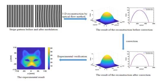
2. Principles

2.1. Introduction of the Brox Optical Flow Algorithm

Brox algorithm, a global method, is a powerful tool for motion analysis. The constraints used in Brox algorithm include the gray value constancy and the gradient constancy, where the latter is particularly helpful for the analysis of translatory motion. The piecewise smooth flow field and multiscale approach are utilized to solve the problem of the discontinuities at the boundaries of objects in the scene and to find the global minimum of the cost functional in a variational formulation in the case of larger displacement.

The brightness of an image point $A_i\left(x_i,y_i\right)$ captured at time t is described by the intensity $I_i\left(x_i,y_i,t\right)$, where subscripts denote the variable on the image plane of the camera. After deformation, point $A_i\left(x_i,y_i\right)$ will move to a new position $B_i\left(x_i+\mathsf{\Delta }{x}_i,y_i+\mathsf{\Delta }{y}_i\right)$ at time $t+\mathsf{\Delta }t$ with intensity ${I^{\prime }}_i\left(x_i+\mathsf{\Delta }{x}_i,y_i+\mathsf{\Delta }{y}_i\right)$. According to the brightness constancy, that is $I_i(x_i,y_i,t)={I^{\prime }}_i\left(x_i+\mathsf{\Delta }{x}_i,y_i+\mathsf{\Delta }{y}_i,t+\mathsf{\Delta }t\right)$, which can be modified with a first-order Taylor approximation, the optical flow constraint equation can be obtained, as shown in Equation (1):

$$\frac{\partial I_i}{\partial x_i}\frac{\mathsf{\Delta }{x}_i}{\mathsf{\Delta }t}+\frac{\partial I_i}{\partial y_i}\frac{\mathsf{\Delta }{y}_i}{\mathsf{\Delta }t}+\frac{\partial I_i}{\partial t}=0$$

(1)

where $u=\frac{\mathsf{\Delta }{x}_i}{\mathsf{\Delta }t}$ and $v=\frac{\mathsf{\Delta }{y}_i}{\mathsf{\Delta }t}$ are the components of the optical flow field between two frames that are the velocity components of the observation point $A_i\left(x_i,y_i\right)$ in x and y directions. Then, the global deviations of the assumption of brightness constancy and gradient constancy and the assumption of the piecewise smooth flow field are measured by an energy expression—shown in Equation (2)—after taking quadratic penalisers into account:

$$\begin{array}{l}E\left(u,v\right)={\displaystyle {\int }_{\mathsf{\Omega }}\mathsf{\Psi }\left({\left|I\left(p+w\right)-I\left(p\right)\right|}^2\right)+\gamma \mathsf{\Psi }\left({\left|\nabla I\left(p+w\right)-\nabla I\left(p\right)\right|}^2\right)dp}\hfill \\ +\alpha {\displaystyle {\int }_{\mathsf{\Omega }}\mathsf{\Psi }\left({\left|\nabla u\right|}^2+{\left|\nabla v\right|}^2\right)dp}\hfill \end{array}$$

(2)

where $\left(x,y\right)\in \mathsf{\Omega }$, $\mathsf{\Omega }$ defines the image domain, $p={\left(x,y\right)}^T$, $w={\left(u,v\right)}^T$, $\gamma$ is the weight between two assumptions and $\alpha$ denotes the regularization parameter greater than 0. $\mathsf{\Psi }\left(x^2\right)=\sqrt{x^2+{\epsilon }^2}$ is an increasing concave function, $\epsilon$ is the small positive constant, which can be chosen as 0.001 [13]. Since Brox optical flow algorithm requires the optical flow itself to be as smooth as possible, it is necessary to find the values of u and v to minimize the energy in Equation (2). Then, the minimizer of Equation (2) must fulfill the Euler–Lagrange equation as follows:

$$\begin{array}{l}{\mathsf{\Psi }}^{\prime }\left(I_z^2\right)I_x{I}_z+\gamma {\mathsf{\Psi }}^{\prime }\left(I_{xz}^2+I_{yz}^2\right)\left(I_{xx}{I}_{xz}+I_{xy}{I}_{yz}\right)-\alpha div\left[{\mathsf{\Psi }}^{\prime }\left(u_x^2+u_y^2+v_x^2+v_y^2\right)\left(u_x{\overrightarrow{e}}_x+u_y{\overrightarrow{e}}_y\right)\right]=0\\ {\mathsf{\Psi }}^{\prime }\left(I_z^2\right)I_y{I}_z+\gamma {\mathsf{\Psi }}^{\prime }\left(I_{xz}^2+I_{yz}^2\right)\left(I_{xy}{I}_{xz}+I_{yy}{I}_{yz}\right)-\alpha div\left[{\mathsf{\Psi }}^{\prime }\left(u_x^2+u_y^2+v_x^2+v_y^2\right)\left(v_x{\overrightarrow{e}}_x+v_y{\overrightarrow{e}}_y\right)\right]=0\end{array}$$

(3)

where ${\mathsf{\Psi }}^{\prime }\left(x^2\right)=\frac{1}{2\sqrt{x^2+{\epsilon }^2}}$, $u_x=\frac{\partial u}{\partial x}$, $u_y=\frac{\partial u}{\partial y}$, $v_x=\frac{\partial v}{\partial x}$, $v_y=\frac{\partial v}{\partial y}$, and ${\stackrel{\rightharpoonup }{e}}_x$ and ${\stackrel{\rightharpoonup }{e}}_y$ are the unit vectors in the x and y axe directions. $I_x=\frac{\partial I\left(p+w\right)}{\partial x}$, $I_y=\frac{\partial I\left(p+w\right)}{\partial y}$, $I_z=I\left(p+w\right)-I\left(p\right)$, $I_{xx}=\frac{{\partial }^{2}I\left(p+w\right)}{\partial x^2}$, $I_{xy}=\frac{{\partial }^{2}I\left(p+w\right)}{\partial x\partial y}$, $I_{yy}=\frac{{\partial }^{2}I\left(p+w\right)}{\partial y^2}$, $I_{xz}=\frac{\partial I\left(p+w\right)}{\partial x}-\frac{\partial I\left(p\right)}{\partial x}$, and $I_{yz}=\frac{\partial I\left(p+w\right)}{\partial y}-\frac{\partial I\left(p\right)}{\partial y}$. Let $w^k={\left(u^k,v^k\right)}^{{\rm T}},k=0,1,\dots$, k represent the number of iterations, then $w^{k+1}$ can be obtained by Equation (4):

$$\begin{array}{l}{\mathsf{\Psi }}^{\prime }\left[{\left(I_z^{k+1}\right)}^2\right]I_x^k{I}_z^{k+1}+\gamma {\mathsf{\Psi }}^{\prime }\left[{\left(I_{xz}^{k+1}\right)}^2+{\left(I_{yz}^{k+1}\right)}^2\right]\left(I_{xx}^k{I}_{xz}^{k+1}+I_{xy}^k{I}_{yz}^{k+1}\right)\\ -\alpha div\left\{{\mathsf{\Psi }}^{\prime }\left[{\left(u_x^{k+1}\right)}^2+{\left(u_y^{k+1}\right)}^2+{\left(v_x^{k+1}\right)}^2+{\left(v_y^{k+1}\right)}^2\right]\left(u_x^{k+1}{\stackrel{\rightharpoonup }{e}}_x+u_y^{k+1}{\stackrel{\rightharpoonup }{e}}_y\right)\right\}=0\end{array}$$

(4)

The first order Taylor expansion is used to remove the nonlinearity in $I^{k+1}$, then,

$$\begin{array}{l}{I}_z^{k+1}\approx I_z^k+I_x^{k}d{u}^k+I_y^{k}d{v}^k\\ I_{xz}^{k+1}\approx I_{xz}^k+I_{xx}^{k}d{u}^k+I_{xy}^{k}d{v}^k\\ I_{yz}^{k+1}\approx I_{yz}^k+I_{xy}^{k}d{u}^k+I_{yy}^{k}d{v}^k\end{array}$$

(5)

where $u^{k+1}$ and $v^{k+1}$ are the velocity components obtained in the iteration k + 1, with k a positive integer, and then represented by $\widehat{u}$ and $\widehat{v}$, respectively. Furthermore, they are expressed as Equation (6), the sum of the result $u^k$ and $v^k$ obtained in the iteration k and the increments $d{u}^k$ and $d{v}^k$ in the iteration k + 1.

$$u^{k+1}=u^k+d{u}^k$$

$$v^{k+1}=v^k+d{v}^k$$

(6)

Substitute Equation (5) into Equation (4); we have

$$\begin{array}{l}\frac{I_x^k\left(I_z^k+I_x^{k}d{u}^k+I_y^{k}d{v}^k\right)}{2\sqrt{{\left(I_z^k+I_x^{k}d{u}^k+I_y^{k}d{v}^k\right)}^2+{\epsilon }^2}}+\frac{\gamma }{2}\frac{I_{xx}^k\left(I_{xz}^k+I_{xx}^{k}d{u}^k+I_{xy}^{k}d{v}^k\right)+I_{xy}^k\left(I_{yz}^k+I_{xy}^{k}d{u}^k+I_{yy}^{k}d{v}^k\right)}{\sqrt{{\left(I_{xz}^k+I_{xx}^{k}d{u}^k+I_{xy}^{k}d{v}^k\right)}^2+{\left(I_{yz}^k+I_{xy}^{k}d{u}^k+I_{yy}^{k}d{v}^k\right)}^2+{\epsilon }^2}}\\ -\frac{\alpha }{2}div\left(\frac{{\widehat{u}}_x{\overrightarrow{e}}_x+{\widehat{u}}_y{\overrightarrow{e}}_y}{\sqrt{{\widehat{u}}_x^2+{\widehat{u}}_y^2+{\widehat{v}}_x^2+{\widehat{v}}_y^2}}\right)=0\end{array}$$

$$\begin{array}{l}\frac{I_y^k\left(I_z^k+I_x^{k}d{u}^k+I_y^{k}d{v}^k\right)}{2\sqrt{{\left(I_z^k+I_x^{k}d{u}^k+I_y^{k}d{v}^k\right)}^2+{\epsilon }^2}}+\frac{\gamma }{2}\frac{I_{xy}^k\left(I_{xz}^k+I_{xx}^{k}d{u}^k+I_{xy}^{k}d{v}^k\right)+I_{yy}^k\left(I_{yz}^k+I_{xy}^{k}d{u}^k+I_{yy}^{k}d{v}^k\right)}{\sqrt{{\left(I_{xz}^k+I_{xx}^{k}d{u}^k+I_{xy}^{k}d{v}^k\right)}^2+{\left(I_{yz}^k+I_{xy}^{k}d{u}^k+I_{yy}^{k}d{v}^k\right)}^2+{\epsilon }^2}}\\ -\frac{\alpha }{2}div\left(\frac{{\widehat{v}}_x{\overrightarrow{e}}_x+{\widehat{v}}_y{\overrightarrow{e}}_y}{\sqrt{{\widehat{u}}_x^2+{\widehat{u}}_y^2+{\widehat{v}}_x^2+{\widehat{v}}_y^2}}\right)=0\end{array}$$

(7)

The first two items in Equation (7) are data items and the third is the smoothness term. Disassemble the data items in Equation (7), let

$$\begin{array}{l}{a}_{11}=\frac{I_x^k{I}_x^k}{2\sqrt{{\left(I_z^k+I_x^{k}d{u}^k+I_y^{k}dv\right)}^2+{\epsilon }^2}}+\frac{\gamma }{2}\frac{I_{xx}^k{I}_{xx}^k+I_{xy}^k{I}_{xy}^k}{\sqrt{{\left(I_{xz}^k+I_{xx}^{k}d{u}^k+I_{xy}^{k}d{v}^k\right)}^2+{\left(I_{yz}^k+I_{xy}^{k}d{u}^k+I_{yy}^{k}d{v}^k\right)}^2}+{\epsilon }^2}\\ a_{12}=\frac{I_x^k{I}_y^k}{2\sqrt{{\left(I_z^k+I_x^{k}d{u}^k+I_y^{k}dv\right)}^2+{\epsilon }^2}}+\frac{\gamma }{2}\frac{I_{xx}^k{I}_{xy}^k+I_{xy}^k{I}_{yy}^k}{\sqrt{{\left(I_{xz}^k+I_{xx}^{k}d{u}^k+I_{xy}^{k}d{v}^k\right)}^2+{\left(I_{yz}^k+I_{xy}^{k}d{u}^k+I_{yy}^{k}d{v}^k\right)}^2}+{\epsilon }^2}\\ b_1=\frac{I_x^k{I}_z^k}{2\sqrt{{\left(I_z^k+I_x^{k}d{u}^k+I_y^{k}dv\right)}^2+{\epsilon }^2}}+\frac{\gamma }{2}\frac{I_{xx}^k{I}_{xz}^k+I_{xy}^k{I}_{yz}^k}{\sqrt{{\left(I_{xz}^k+I_{xx}^{k}d{u}^k+I_{xy}^{k}d{v}^k\right)}^2+{\left(I_{yz}^k+I_{xy}^{k}d{u}^k+I_{yy}^{k}d{v}^k\right)}^2}+{\epsilon }^2}\\ a_{21}=\frac{I_x^k{I}_y^k}{2\sqrt{{\left(I_z^k+I_x^{k}d{u}^k+I_y^{k}dv\right)}^2+{\epsilon }^2}}+\frac{\gamma }{2}\frac{I_{xx}^k{I}_{xy}^k+I_{xy}^k{I}_{yy}^k}{\sqrt{{\left(I_{xz}^k+I_{xx}^{k}d{u}^k+I_{xy}^{k}d{v}^k\right)}^2+{\left(I_{yz}^k+I_{xy}^{k}d{u}^k+I_{yy}^{k}d{v}^k\right)}^2}+{\epsilon }^2}\\ a_{22}=\frac{I_y^k{I}_y^k}{2\sqrt{{\left(I_z^k+I_x^{k}d{u}^k+I_y^{k}dv\right)}^2+{\epsilon }^2}}+\frac{\gamma }{2}\frac{I_{xy}^k{I}_{xy}^k+I_{yy}^k{I}_{yy}^k}{\sqrt{{\left(I_{xz}^k+I_{xx}^{k}d{u}^k+I_{xy}^{k}d{v}^k\right)}^2+{\left(I_{yz}^k+I_{xy}^{k}d{u}^k+I_{yy}^{k}d{v}^k\right)}^2}+{\epsilon }^2}\\ b_2=\frac{I_y^k{I}_z^k}{2\sqrt{{\left(I_z^k+I_x^{k}d{u}^k+I_y^{k}dv\right)}^2+{\epsilon }^2}}+\frac{\gamma }{2}\frac{I_{xy}^k{I}_{xz}^k+I_{yy}^k{I}_{yz}^k}{\sqrt{{\left(I_{xz}^k+I_{xx}^{k}d{u}^k+I_{xy}^{k}d{v}^k\right)}^2+{\left(I_{yz}^k+I_{xy}^{k}d{u}^k+I_{yy}^{k}d{v}^k\right)}^2}+{\epsilon }^2}\end{array}$$

(8)

Then, the data items in Equation (7) can be simplified as:

$$\begin{array}{l}{a}_{11}d{u}^k+a_{12}d{v}^k=-b_1\\ a_{21}d{u}^k+a_{22}d{v}^k=-b_2\end{array}$$

(9)

Let $\varphi \left(x,y\right)=\frac{\alpha /2}{\sqrt{{\widehat{u}}_x^2+{\widehat{u}}_y^2+{\widehat{v}}_x^2+{\widehat{v}}_y^2}}$, then $b_1$, $b_2$, $a_{11}$ and $a_{22}$ can be expressed as:

$$\begin{array}{l}{b}_1=b_1+\left\{\begin{array}{l}\left[u^k\left(x,y\right)-u^k\left(x-1,y\right)\right]\varphi \left(x-1,y\right)-\left[u^k\left(x+1,y\right)-u^k\left(x,y\right)\right]\varphi \left(x,y\right)\\ +\left[u^k\left(x,y\right)-u^k\left(x,y-1\right)\right]\varphi \left(x,y-1\right)-\left[u^k\left(x,y+1\right)-u^k\left(x,y\right)\right]\varphi \left(x,y\right)\end{array}\right\}\\ b_2=b_2+\left\{\begin{array}{l}\left[v^k\left(x,y\right)-v^k\left(x-1,y\right)\right]\varphi \left(x-1,y\right)-\left[v^k\left(x+1,y\right)-v^k\left(x,y\right)\right]\varphi \left(x,y\right)\\ +\left[v^k\left(x,y\right)-v^k\left(x,y-1\right)\right]\varphi \left(x,y-1\right)-\left[v^k\left(x,y+1\right)-v^k\left(x,y\right)\right]\varphi \left(x,y\right)\end{array}\right\}\\ a_{11}=a_{11}+\varphi \left(x-1,y\right)+\varphi \left(x,y\right)+\varphi \left(x,y-1\right)+\varphi \left(x,y\right)\\ a_{22}=a_{22}+\varphi \left(x-1,y\right)+\varphi \left(x,y\right)+\varphi \left(x,y-1\right)+\varphi \left(x,y\right)\end{array}$$

(10)

Finally, the increments $d{u}^{k+1}$ and $d{v}^{k+1}$ can be obtained by using the SOR iteration method [16]:

$$\begin{array}{l}d{u}^{k+1}=\left(1-\omega \right)d{u}^k+\frac{\omega }{a_{11}}\left[b_1-a_{12}d{v}^k+\left(\begin{array}{l}d{u}^k\left(x-1,y\right)\varphi \left(x-1,y\right)+d{u}^k\left(x+1,y\right)\varphi \left(x,y\right)\\ +d{u}^k\left(x,y-1\right)\varphi \left(x,y-1\right)+d{u}^k\left(x,y+1\right)\varphi \left(x,y+1\right)\end{array}\right)\right]\\ d{v}^{k+1}=\left(1-\omega \right)d{v}^k+\frac{\omega }{a_{22}}\left[b_2-a_{21}d{u}^k+\left(\begin{array}{l}d{v}^k\left(x-1,y\right)\varphi \left(x-1,y\right)+d{v}^k\left(x+1,y\right)\varphi \left(x,y\right)\\ +d{v}^k\left(x,y-1\right)\varphi \left(x,y-1\right)+d{v}^k\left(x,y+1\right)\varphi \left(x,y+1\right)\end{array}\right)\right]\end{array}$$

(11)

where $\omega$ is the relaxation parameter in the SOR iteration method. $a_{11}$, $a_{22}$, $b_1$ and $b_2$ can be obtained after the initial values are given to $u$, $v$, $du$ and $dv$. The iterative calculation using Equation (11) can be terminated until the difference of the calculation between two adjacent iterations approaches 0. Then, the optical flow fields u and v can be obtained using Equation (6). Experiment results show that Brox optical flow algorithm has the advantages of running fast, is suitable for larger displacement and is better robust to noises.

2.2. The Principle of the Surface Shape Measurement

Figure 1 shows the diagram of surface shape measurement using the optical flow method. A projector at point $P\left(x_p,y_p,z_p\right)$ projects a pattern onto the reference plane N, where a measured surface S can be placed. A camera located at point $C\left(x_c,y_c,z_c\right)$ captures the projected pattern on the measured surface. The projection optical axis PO rays from the projector to the reference plane at an angle $\theta$ with respect to the normal of the reference plane and crosses the plane at O, which is set as the origin of the coordinate system established on the reference plane. Take the line $P_{\perp }O$ as the x-axis direction, where $P_{\perp }$ represents the foot of the perpendicular $P{P}_{\perp }$ on the reference plane, and the normal of the reference plane at point O as the z-axis direction. The optical axis $C{C}_{\perp }$ of the CCD camera is perpendicular to the reference plane, and the foot point is $C_{\perp }$. The distance $\overline{C{C}_{\perp }}$ is the observation distance, represented by $z_c$. These coordinate position parameters of the projector and the camera can be calibrated using the calibration method.

Observing a point $A(x,y)$ on the reference plane, the projection light $\overrightarrow{PA}$ will meet the point D on the surface after placing the measured object. The height of the point D is h. In other words, the observation point $A(x,y)$ moves to a new position $B(x^{\prime },y^{\prime })$ after the time $\mathsf{\Delta }t$ due to the existence of the object. The displacements between two points are $\mathsf{\Delta }x=x^{\prime }-x$ and $\mathsf{\Delta }y=y^{\prime }-y$. Then, the point $A_i\left(x_i,y_i\right)$ moves to $B_i\left(x_i+\mathsf{\Delta }{x}_i,y_i+\mathsf{\Delta }{y}_i\right)$ on image plane, corresponding to the point $A(x,y)$ and $B(x^{\prime },y^{\prime })$, where $\mathsf{\Delta }{x}_i$ and $\mathsf{\Delta }{y}_i$ are the displacement in the x and y direction. The relations of the displacement between them are $\mathsf{\Delta }{x}_i=M_c\mathsf{\Delta }x$ and $\mathsf{\Delta }{y}_i=M_c\mathsf{\Delta }y$, where $M_c$ is the image magnification. The optical flow formed by deformation is the velocity components at the point $A_i\left(x_i,y_i\right)$, can be expressed as:

$$u=\frac{\mathsf{\Delta }{x}_i}{\mathsf{\Delta }t}=M_c\frac{\mathsf{\Delta }x}{\mathsf{\Delta }t}, v=\frac{\mathsf{\Delta }{y}_i}{\mathsf{\Delta }t}=M_c\frac{\mathsf{\Delta }y}{\mathsf{\Delta }t}$$

(12)

where the time interval between two captured frames, $\mathsf{\Delta }t$, usually set as 1 for convenience in calculation because of no limitation on it.

In order to find the relationship between the deformation of the fringes and the height of the object surface, geometric analysis is performed as follows. First, use the coordinates of the projector and the camera to show some important lengths of the line segments in the measurement system:

$$\begin{array}{c}\hfill d_{AP}=\sqrt{{\left(x-x_p\right)}^2+{\left(y-y_p\right)}^2+z_p^2}\hfill \\ \hfill d_{BP}=\sqrt{{\left(x^{\prime }-x_p\right)}^2+{\left(y^{\prime }-y_p\right)}^2+z_p^2}\hfill \\ \hfill d_{AB}=\sqrt{{\left(x-x^{\prime }\right)}^2+{\left(y-y^{\prime }\right)}^2}\hfill \\ \hfill d_{AC}=\sqrt{{\left(x-x_c\right)}^2+{\left(y-y_c\right)}^2+z_c^2}\hfill \\ \hfill d_{CP}=\sqrt{{\left(x_p-x_c\right)}^2+{\left(y_p-y_c\right)}^2+{\left(z_p-z_c\right)}^2}\hfill \end{array}$$

(13)

where $x^{\prime }=x+\mathsf{\Delta }x=x+u\mathsf{\Delta }t/M_c$ and $y^{\prime }=y+\mathsf{\Delta }y=y+v\mathsf{\Delta }t/M_c$. Then, passing through point C, draw an auxiliary plane M parallel to the reference plane N. Extend the line AP to intersect the plane M at point $P^{\prime }$. Geometrically, we know that $P^{\prime }C//AB$ due to point, $P^{\prime }$, $C$, $A$ and $B$, are coplanar. On the plane $P^{\prime }CAB$, the cosines of $\angle PAB$ and $\angle CPA$ are shown in Equation (14) using the law of cosines:

$$\cos \angle PAB=\frac{d_{AP}^2+d_{AB}^2-d_{BP}^2}{2d_{AP}{d}_{AB}},\cos \angle CPA=\frac{d_{CP}^2+d_{AP}^2-d_{AC}^2}{2d_{CP}{d}_{AP}}$$

(14)

and

$$\angle CP{P}^{\prime }=\pi -\angle CPA, \angle C{P}^{\prime }P=\angle PAB$$

(15)

Then, the length of the line segment $C{P}^{\prime }$ can be expressed by the cosines of $\angle PAB$ and $\angle CPA$ using the sine theorem:

$$d_{C{P}^{\prime }}=d_{CP}\frac{\sin \angle CP{P}^{\prime }}{\sin \angle C{P}^{\prime }P}=d_{CP}\frac{\sqrt{1-{\cos }^2\angle CP{P}^{\prime }}}{\sqrt{1-{\cos }^2\angle C{P}^{\prime }P}}$$

(16)

The height at point D can be expressed as:

$$h=\frac{d_{AB}\cdot z_c}{d_{C{P}^{\prime }}+d_{AB}}$$

(17)

Substitute Equations (13)–(15) into Equation (17); the expression of the height h of point D can be obtained:

$$h=\frac{z_c\sqrt{d_{AB}^2[2(d_{AP}^2+d_{BP}^2)-d_{AB}^2]-{[d_{AP}^2-d_{BP}^2]}^2}}{\sqrt{d_{AB}^2[2(d_{AP}^2+d_{BP}^2)-d_{AB}^2]-{[d_{AP}^2-d_{BP}^2]}^2}+\sqrt{d_{AC}^2[2(d_{AP}^2+d_{CP}^2)-d_{AC}^2]-{[d_{AP}^2-d_{CP}^2]}^2}}$$

(18)

Usually, the foot of the CCD camera on reference plane, $C_{\perp }$, is used as the origin of the coordinate system, and let the projection center coincide with the observation center in experiment.

2.3. Correction Principle

In the actual measurement, usually, the optical center of the projector is not at the same height as that of the camera, which results in the inconsistent measured result with that of the actual object. In this section, we propose a correction method to solve the problem in the optical flow method.

For the sake of simplicity, Figure 1 is simplified into a 2-D coordinate system. As shown in Figure 2, the optical center of the projector is at the same height as that of the camera completely. Consider two points, $D$ and $D^{\prime }$, which are at the same height $h$ on the surface of the measured object. When the two points are observed by the camera, the magnitudes of the displacement at the two points caused by the same height are different. Let $\mathsf{\Delta }{x}_1$ and $\mathsf{\Delta }{x}_2$ represent the displacement caused by h at point $D$ and $D^{\prime }$, respectively. Then, we have

$$\frac{h}{z_c-h}=\frac{\mathsf{\Delta }{x}_1}{d}=\frac{\mathsf{\Delta }{x}_2}{d}$$

(19)

where $d=\left|x_p-x_c\right|$ is the distance between the projector and the camera. It is easy to obtain that

$$\mathsf{\Delta }{x}_1=\mathsf{\Delta }{x}_2$$

(20)

It can be seen from Equation (20) that the horizontal component of the optical flow $u$ at point $D$ is also equal to that at point $D^{\prime }$. However, in practice, it is difficult to make the optical center of the projector at exactly the same height as that of the camera. Once the optical center $P^{\prime }$ and $C$ are not on the same horizontal line, $\mathsf{\Delta }{x}_1$ will no longer be equal to $\mathsf{\Delta }{x}_2$, resulting in a height deviation in the calculated value.

As shown in Figure 3, we can think of the projector moving from P′ to P. Then, there is a displacement $\mathsf{\Delta }{p}_z$ in the vertical direction and $\mathsf{\Delta }{p}_x$ in the horizontal direction relative to the position $P^{\prime }$. The projection line that hits D will meet point $A(x,y)$ on the reference plane at an incident angle $\alpha$ with respect to the normal of the reference plane. A displacement would be introduced due to the measured surface when the point D is observed from the CCD sensor, which is represented by $\mathsf{\Delta }x$. From the analyses above, we know that there are no deviation errors when the projector is located at the point $P^{\prime }$ horizontal to the CCD optical center. Therefore, the corrected displacement $\mathsf{\Delta }{x}^{\prime }$ can be obtained after finding the small offset $\delta$ caused by the movement of the projector.

As can be seen from Figure 3 that

$$\mathsf{\Delta }{p}_x=\mathsf{\Delta }{p}_z\cdot \tan \alpha =\mathsf{\Delta }{p}_z\cdot \frac{x+d}{z_c}$$

(21)

and

$$\delta =\frac{h\cdot \mathsf{\Delta }{p}_z}{z_c-h}\cdot \frac{x+d}{z_c}$$

(22)

Then, the corrected displacement can be expressed as:

$$\mathsf{\Delta }{x}^{\prime }=\mathsf{\Delta }x+\delta =\mathsf{\Delta }x+\frac{h\cdot \mathsf{\Delta }{p}_z}{z_c-h}\cdot \frac{x+d}{z_c}$$

(23)

where $\mathsf{\Delta }x=u\cdot \mathsf{\Delta }t/M_c$, which is calculated from the optical flow method. The height of the point D is H after modification, is expressed as:

$$H=\frac{\mathsf{\Delta }{x}^{\prime }\cdot z_c}{d+\mathsf{\Delta }{x}^{\prime }}=\frac{z_c[z_c(z_c-h)\mathsf{\Delta }x+(x+d)h\mathsf{\Delta }{p}_z]}{z_c(z_c-h)(\mathsf{\Delta }x+d)+(x+d)h\mathsf{\Delta }{p}_z}$$

(24)

Using Equation (24), the correction of the measurement result and the surface shape information of the object can be retrieved with high precision by using the proposed method, avoiding the problem of the tilt error.

3. Theoretical Simulation

3.1. Numerical Simulation and Analysis of Surface Shape Measurement by Optical Flow Method

The height distribution of the measured surface can be calculated by using Equation (18) and its tilt error can be corrected by using Equation (24). It can be found that there are no restrictions on projection patterns. First, we use the usual parallel projection fringe pattern for shape measurement in simulations and experiments. Then, speckle patterns are proved to be feasible in experiments.

A spherical crown of the size 40 × 40 mm simulated by MATLAB is set to be measured, as shown in Figure 4. The radius of the sphere $R$ is 20 mm and the maximum of its height $h_{\max }$ is 10 mm. The height of the spherical crown is expressed as

$$h(x,y)=-(R-h_{\max })+\sqrt{R^2-x^2-y^2}$$

(25)

The system shown in Figure 1 is employed to measure the shape of the spherical crown. The imaging distance of the camera $z_c$ and the projection distance $z_p$ are 2000 mm, respectively. The distance between projection and the camera d is 60 mm and the image magnification $M_c$ is −12.8 pixel/mm. The optical center of the projector can be considered to be approximately at the same height as that of the camera due to the small projection angle. Before placing the object, the light intensity of the projection fringes parallel to the y-axis direction on the reference plane can be expressed as

$$I(x,y,t)=a+b\cos [2\pi (f_{x}x+f_{y}y)]$$

(26)

where a is the background light intensity, b is the fringe contrast, $f_x$ and $f_y$ are the fringe frequencies at $(x,y)$. The image captured by the CCD camera at time t is expressed as

$$I_i(x_i,y_i,t)=a+b\cos [2\pi (f_{ix}{x}_i+f_{iy}{y}_i)]$$

(27)

where $f_{ix}=f_x/M_c$ and $f_{iy}=f_y/M_c$ are the fringe frequencies of the recorded image, The subscript i represents the physical parameters on the image plane. After placing the object, the light intensity of the modulated fringe image captured at time $t+\mathsf{\Delta }t$ is

$${I^{\prime }}_i(x_i+\mathsf{\Delta }{x}_i,y_i+\mathsf{\Delta }{y}_i,t+\mathsf{\Delta }t)=a+b\cos 2\pi [f_{ix}(x_i+\mathsf{\Delta }{x}_i)+f_{iy}(y_i+\mathsf{\Delta }{y}_i)]$$

(28)

According to Equations (27) and (28), the captured fringe patterns before and after deformation are of size 512 × 512 pixels—shown in Figure 5a,b—respectively, where a = 128, b = 60, $f_{ix}=0.4 {\mathrm{mm}}^{-1}$, $f_{iy}=0$. The fringe deformation is small due to the small distance d between the projector and CCD, and the maximum of deformation in the deformed pattern is 4 pixels.

By using the two images shown in Figure 5, the Brox optical flow algorithm is employed to estimate the optical flow field. In the calculation of the optical flow, the weight factor $\gamma$ is 10, and the regularization parameter $\alpha$ is 100, which can make the algorithm robust to noise, suggested by Brox [13]. Then, the height distribution of the ball crown can be obtained using Equation (18). The result is shown in Figure 6a. Using two fringe patterns to obtain the height distribution in the optical flow method, it is similar to that of the FTP method. Therefore, the height distribution is recalculated by using the FTP method for comparison. The cross section data at y = 0 mm in x direction obtained by the optical flow method and the FTP method are compared with those of the true value, as shown in Figure 6b. It can be seen that both results of the two methods are close to the real value, indicating that the optical flow method has high precision in the surface shape measurement as good as that of the FTP method under the same condition.

The random noise has a great influence on the measurement results. Then, the fringe patterns before and after deformation are polluted by the Gaussian noises with the SNR of 10 and 20 dB, respectively, to simulate the influence of the environmental noises and the thermal noises of the camera. By using the noised fringe patterns, the height distributions of the ball crown are obtained. Then, the distributions of the absolute error are obtained modulo subtracting the cross section data of the calculated results from the true value at y = 0 mm in x direction, as shown in Figure 7. It can be seen that the absolute errors are less than 0.2 mm compared with the noiseless pattern when the noised pattern with SNR is of 10 and 20 dB, respectively. The root mean square (RMS) errors increases with the noise and its maximum value is less than 0.15 mm. It shows that the Brox optical flow algorithm has good robustness to noises.

In the simulations above, the parameters in the measurement system such as $z_p$, $z_c$ and d are constants, which are set as $z_p=2000$ mm,$z_c=2000$ mm and $d=60$ mm, respectively. However, in the actual experiment, these parameters need to be calibrated by optical methods, which may cause errors. In order to explain the impact of calibration error on the calculation results, a incremental 5 mm is firstly added to the observation distance $z_c$ and the projection distance $z_p$, respectively, as the calibration error when $d=60$ mm. Then, increase d by 5 mm when $z_p$ and $z_c$ are both 2000 mm. The absolute errors of 5 mm increments are compared with its original distance, as shown in Figure 8, respectively. It can be seen that the increases of 5 mm in the observation distance and projection distance have little effect on the measurement results. Although the change in d has an obvious effect on the error distribution compared with the first two parameters, the absolute error is still within a small range. So, we can ignore the error caused by the system calibration in the experiment. Furthermore, the parameter d is closely related to the amount of deformation of the projected pattern, which can affect the accuracy of the optical flow algorithm. Therefore, we should make d small enough in experiments.

3.2. Error Correction Simulation

In Section 3.1, the situations are completed when the projector is at the same height as that of the camera. In this section, we consider the case that the observation distance is not equal to the projection distance. When the projection angle $\theta =\pi /100$, the observation distance $z_c$ and the projection distance $L_p$ are set as 2000 and 1800 mm, respectively, the move component of the projector $\mathsf{\Delta }{p}_y$ in vertical direction is about −200 mm. Then, a tilt error occurs due to the deviation of the projector. As shown in Figure 9a, the cross section data of the calculated height distribution is deviated from the true value at y = 0 mm in x direction. The tilt error can be corrected using Equation (24), as shown in Figure 9b. After correction, the absolute error between the calculated value and the true value can be greatly reduced to 0.3 mm, as shown in Figure 9c, indicating that the proposed correction method is feasible.

3.3. Sensitivity Analysis

The sensitivity of a system can be intuitively understood as the change of the output caused by a certain amount of input change. Based on the triangulation method, the optical setup of the proposed method is just like that of the PMP method. Then, the sensitivity of the method can be defined as

$$S=d(\mathsf{\Delta }{x}_i)/dh$$

(29)

We can use Figure 2 to analyze the sensitivity of this method. According to Equation (17), the deformation of the fringe on image plane caused by h is

$$\mathsf{\Delta }{x}_i=M_c\frac{h\cdot d}{z_c-h}$$

(30)

Then, Equation (29) can be approximately expressed as $S=M_c\cdot d/z_c$ when the measured height is far less than $z_c$. We can obtain that the sensitivity of the method is about 0.4 pixel/mm at the maximum height of the ball crown. The proposed method requires the incidence angle small enough to ensure that the deformation of the fringes can be measured by the optical flow method. Small angle projection can avoid shadows of the measured object, but it reduces the sensitivity of measurement. According to the reported resolution of 0.01 pixel in the horizontal direction in the optical flow method [10], the resolution in the direction of height is about 0.02 mm. This resolution is sufficient for most measurements.

4. Experiment

4.1. An Experiment on a Smooth Measuring Object

The measurement system as shown in Figure 1 is utilized to measure the height distribution of the specimen, as shown in Figure 10. The maximum height of the mask is 63.20 mm. The projected pattern used in the proposed optical flow method is not limited to the fringe pattern. Usually, a parallel fringe pattern is utilized to measure the surface shape in current techniques including the FTP method. Therefore, the fringe pattern is firstly used for projection in this section to facilitate comparison with the FTP method. According to the discussion above, the deformation of the deformed fringes should be small to meet the brightness constant of optical flow. Therefore, the projection angle should be small in the setup. Then, the measurement follows the following steps:

• Calibrating the measurement system. In order to make the effect of the correction method obvious, we set the projection distance and observation distance with large distance. Different from the optical setup parameter estimation method [17], the optical center positions of the projector and camera are calibrated by using Zhang’s calibration method [18,19]. After calibration, the distance from the projector to the reference plane is 1975.40 mm and that of the CCD sensor is 1922.80 mm. The horizontal distance between the CCD sensor and the projector is 84.50 mm. The magnification of the image is 512/220 pixel/mm. The calibration process will take about 10 min, but the following steps can be performed multiple times as long as the calibration is completed once.
• Capturing two images. The two images before and after placing the object are recorded by an ordinary CCD sensor with the sensitive area of 768 × 576 pixels at 8-bit resolution. The captured images are shown in Figure 11. We estimate the noise level of the image by using the method proposed by Chen et al. [20]. The mean noise level of Figure 11b is 1.41 dB.
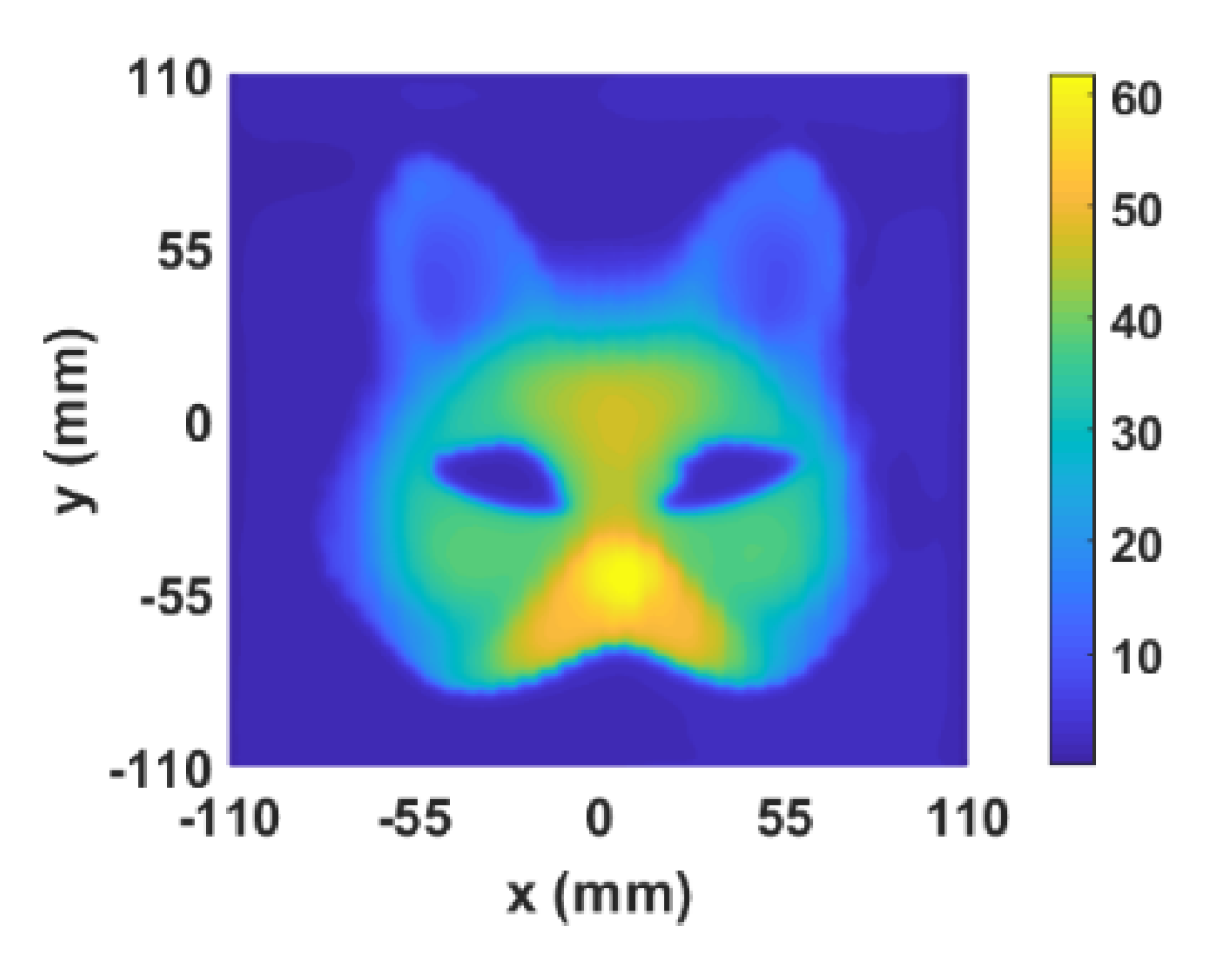
• Calculating the optical flow and height distribution. After calculating the optical flow between the two images by using the Brox method, the height distribution of the specimen can be obtained according to Equation (18)—shown in Figure 12. This step will take 6 to 10 s depending on the image size and the parameters of Brox algorithm.

It should be noted that the location of the projector is 52.60 mm farther than that of the CCD sensor to the reference plane. This would introduce a tilt error in the measurement result. The tilt error can be corrected according to Equation (24). The corrected result is shown in Figure 13a.

In order to show the effect of the correction, the cross section data of the corrected result at y=-20 mm in x direction (passing through the hollow area of the object) are compared with those of the uncorrected result, as shown in Figure 13b. To compare with the result before correction, the correction effect is obvious and satisfactory. First, the maximum of the height is 62.19 mm after correction. At the maximum height, the absolute error of the corrected measurement results is 1.01 mm and the relative error is less than 2%. Second, the height distribution becomes left-right symmetric after correction. The tilt error occurs in calculated height distribution before correction has been greatly reduced.

As described in Section 3.1, the proposed method has no restrictions on projection patterns, which is illustrated by an experiment with projected speckle patterns. Using the measurement system shown in Figure 1 and the same parameters as the experiment in Section 4.1, the height distributions of the specimen are obtained using Equation (18) following the experimental steps described above. Figure 14 shows the height distribution of the specimen using the projected speckle pattern.

The Brox method is slightly similar to the FTP method in the calculation of using the fringe patterns before and after deformation. Therefore, the height distribution of the specimen is recalculated by the FTP method. After transforming the two fringe patterns into their frequency domain using the fast Fourier transform algorithm, calculating the carrier frequency, selecting one of the spectra on the frequency axis by a window manually and translating it, inverse Fourier transform and phase unwrapping are necessary to obtain the phase distribution of the measured surface. Then, the transformation of phase-to-height is required in order to obtain the height distribution. After completing the operations above, the height distribution of the specimen can be obtained—shown in Figure 15a—from which the cross section data at y = −20 mm in x direction are selected to compare with that of the corrected Brox method. The comparison of them is shown in Figure 15b. It can be found that the result of the corrected Brox method is more accurate than that of the FTP method.

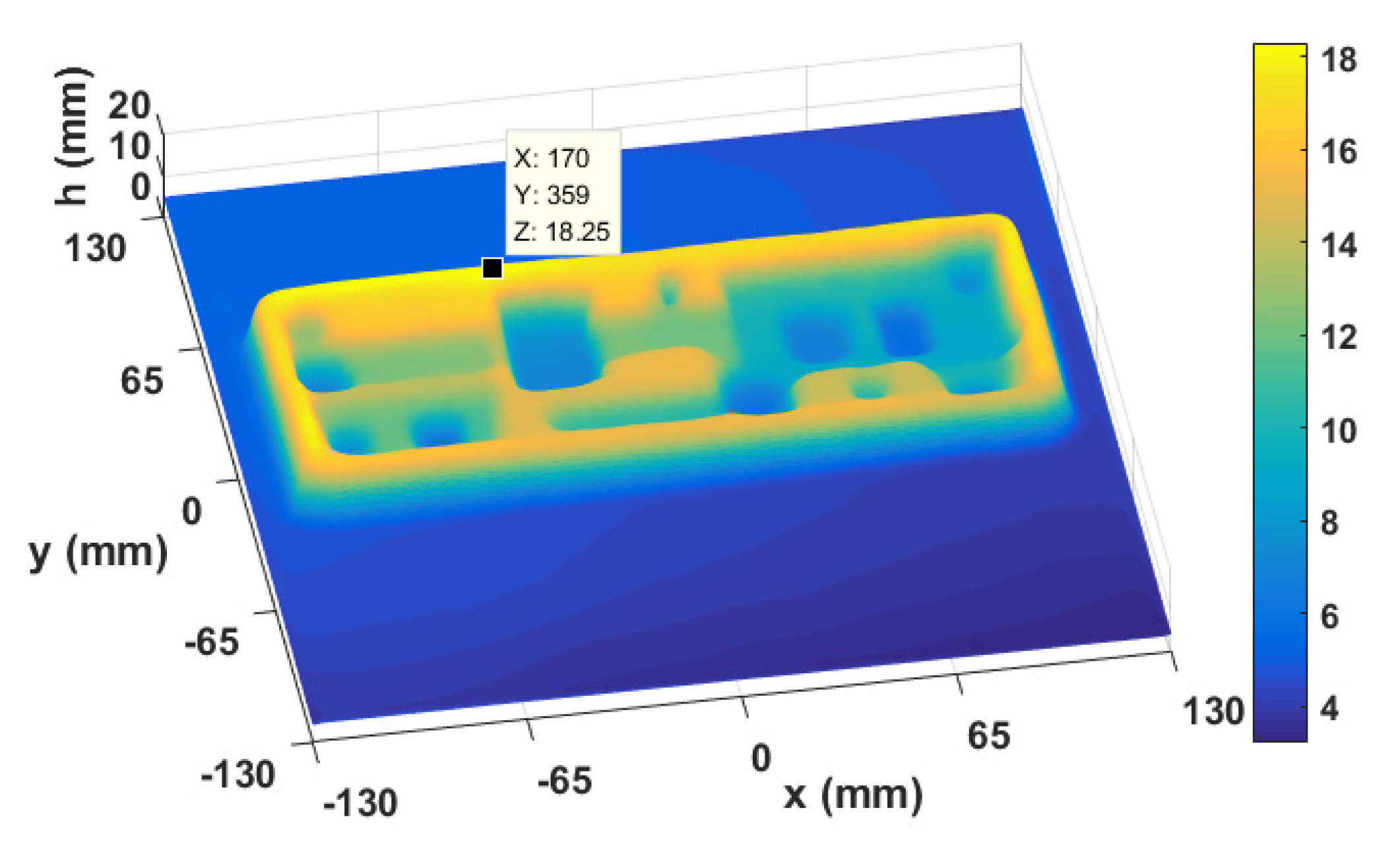
4.2. An Experiment on a Structured Object

In Section 3.1, we measure an object with a smooth surface. To illustrate the feasibility of the proposed approach, a packaging box of an instrument is measured. The packaging box is of structured surfaces, as shown in Figure 16. Its maximum height is 18.20 mm. The mean noise level of the captured image is 2.86 dB, also estimated by Chen’s method. The corrected measurement result is shown in Figure 17, where the maximum of the measured height is 18.25 mm. The absolute error and relative error at the point are 0.05 mm and 0.3%, respectively. The experimental result show that the proposed method is suitable for 3-D reconstruction of objects with structural surface.

Although the experimental result is satisfactory, the accuracy of it may not be as high as that of PMP method. However, the advantages of the proposed method are obvious and potential. Firstly, the measurement time is much shorter than that of the PMP method because only two images are required. Secondly, the height distribution is obtained directly without phase calculation like the PMP method. Finally, a more diversified pattern can be used for projection in the proposed method, such as speckle pattern, which is difficult for data processing in the PMP method. Moreover, the proposed method based on the optical flow is more suitable for dynamic measurement.

5. Conclusions

In this paper, a new technique for measuring the surface shape of an object based on the Brox optical flow method is presented. The measurement system is simple with one projector and a CCD sensor. Because of the small projection angle, the shadow problem is avoided. The proposed method has no restrictions on projection patterns. Due to the tilt error that exists in the measurement results, an error correction method for the optical flow method is proposed, by which the height distribution can be accurately measured. Simulations and experiments are completed to demonstrate the characteristics of the proposed method. The result shows that the Brox optical flow algorithm has good robustness to noises. It also shows that the measurement results are not sensitive to the deviation of projection distance and observation distance. The deviation of 5mm of the projection distance or observation distance has little influence on the measurement results. However, it is sensitive to the distance between the projector and the CCD sensor. Comparing with the Fourier transform method, the proposed method is simple in the calculation of the height distribution without phase-to-height transformation. The height calculation process does not require manual intervention. Only two images are needed to obtain the height distribution. Therefore, the proposed method is more suitable for dynamic measurement. However, there are still some problems that need to be discussed further, such as the influence of the background and the color inconsistency between the measured object and the reference plane. These problems would be studied in the future.

References

1. Godin, G.; Beraldin, J.A.; Taylor, J.; Cournoyer, L.; Rioux, M.; El-Hakim, S.; Baribeau, R.; Blais, F.; Boulanger, P.; Domey, J.; et al. Active optical 3D imaging for heritage applications. IEEE. Comput. Graph 2002, 22, 24–36. [Google Scholar] [CrossRef]
2. Yue, L.; Liu, X. Application of 3D optical measurement system on quality inspection of turbine blade. In Proceedings of the 2009 16th International Conference on Industrial Engineering and Engineering Management, Beijing, China, 21–23 October 2009; pp. 1089–1092. [Google Scholar]
3. Hung, Y.; Lin, L.; Shang, H.; Park, B.G. Practical three-dimensional computer vision techniques for full-field surface measurement. Opt. Eng. 2000, 39, 143. [Google Scholar] [CrossRef]
4. Fitts, J.M. High-Speed 3-D Surface Measurement Surface Inspection and Reverse-CAD System. U.S. Patent 5,175,601, 29 December 1992. [Google Scholar]
5. Gorthi, S.S.; Rastogi, P. Fringe projection techniques: Whither we are? Opt. Lasers Eng. 2010, 48, 133–140. [Google Scholar] [CrossRef] [Green Version]
6. Takeda, M.; Ina, H.; Kobayashi, S. Fourier-transform method of fringe-pattern analysis for computer-based topography and interferometry. J. Opt. Soc. Am. 1982, 72, 156–160. [Google Scholar] [CrossRef]
7. Yang, F.; He, X. Two-step phase-shifting fringe projection profilometry: Intensity derivative approach. Appl. Opt. 2007, 46, 7172. [Google Scholar] [CrossRef] [PubMed]
8. Yao, J.; Tang, Y.; Chen, J. Three-dimensional shape measurement with an arbitrarily arranged projection moiré system. Opt. Lett. 2016, 41, 717–720. [Google Scholar] [CrossRef] [PubMed]
9. Sun, P.; Dai, Q.; Tang, Y.; Lei, Z. Coordinate calculation for direct shape measurement based on optical flow. Appl. Opt. 2020, 59, 92–96. [Google Scholar] [CrossRef] [PubMed]
10. Hartmann, C.; Wang, J.; Opristescu, D.; Volk, W. Implementation and evaluation of optical flow methods for two-dimensional deformation measurement in comparison to digital image correlation. Opt. Lasers Eng. 2018, 107, 127–141. [Google Scholar] [CrossRef]
11. Li, B.; Fu, Y.; Zhang, J.; Wu, H.; Zeng, Z. Period correction method of phase coding fringe. Opt. Rev. 2015, 22, 717–723. [Google Scholar] [CrossRef]
12. Wang, Z.; Du, H.; Bi, H. Out-of-plane shape determination in generalized fringe projection profilometry. Opt. Express 2006, 14, 12122–12133. [Google Scholar] [CrossRef] [PubMed]
13. Brox, T.; Bruhn, A.; Papenberg, N.; Weickert, J. High accuracy optical flow estimation based on a theory for warping. In European Conference on Computer Vision; Springer: Berlin/Heidelberg, Germany, 2004; pp. 25–36. [Google Scholar]
14. Horn, B.K.P.; Schunck, B.G. Determining optical flow. Artif. Intell. 1981, 17, 185–203. [Google Scholar] [CrossRef] [Green Version]
15. Lucas, B.; Kanade, T. An iterative image registration technique with an application to stereo vision. In Proceedings of the 7th International Joint Conference on Artificial Intelligence (IJCAI’), San Francisco, CA, USA, 24–28 August 1981. [Google Scholar]
16. Xing-Jiang, L.; Lai-I, L. Geometric interpretation of several classical iterative methods for linear system of equations and diverse relaxation parameter of the SOR method. Appl. Math. J. Chin. Univ. 2013, 28, 269–278. [Google Scholar]
17. Kofman, J. Comparison of linear and nonlinear calibration methods for phase-measuring profilometry. Opt. Eng. 2007, 46, 043601. [Google Scholar] [CrossRef]
18. Zhang, Z. A flexible new technique for camera calibration. IEEE. Trans. Pattern Anal. 2000, 22, 1330–1334. [Google Scholar] [CrossRef] [Green Version]
19. An, Y.; Bell, T.; Li, B.; Xu, J.; Zhang, S. Method for large-range structured light system calibration. Appl. Opt. 2016, 55, 9563–9572. [Google Scholar] [CrossRef] [PubMed]
20. Chen, G.; Zhu, F.; Heng, P.A. An Efficient Statistical Method for Image Noise Level Estimation. In Proceedings of the 2015 IEEE International Conference on Computer Vision (ICCV), Santiago, Chile, 7–13 December 2015. [Google Scholar]
Figure 1. The diagram of surface shape measurement using optical flow method.
Photonics 07 00109 g001
Figure 2. The simplified optical setup when the projector is at the same height as that of the camera.
Photonics 07 00109 g002
Figure 3. The diagram of the error correction when the center of the camera is not the same as that of the projector.
Photonics 07 00109 g003
Figure 4. The spherical crown to be measured.
Photonics 07 00109 g004
Figure 5. The captured fringe patterns: (a) before deformation and (b) after deformation.
Photonics 07 00109 g005
Figure 6. (a) The calculated height distribution of the spherical crown. (b) The comparison of the cross section data between the calculated value and true value at y = 0 mm in x direction.
Photonics 07 00109 g006
Figure 7. The error analysis of the proposed method. (a) The absolute error and (b) RMS error of the calculated on the cross section data at y = 0 mm in x direction when the fringe patterns are polluted by the Gaussian noises with SNR of 10 and 20 dB, respectively.
Photonics 07 00109 g007
Figure 8. The influence of various parameters in the simulation. The comparison of the absolute error between the cross section data at y = 0 mm in x direction in the calculated height distribution before and after (a) z c increase by 5 mm, (b) z p increase by 5 mm and (c) d increase by 5 mm.
Photonics 07 00109 g008
Figure 9. The comparison of the cross section data between the calculated and true value at y = 0 mm in x direction (a) before correction and (b) after correction. (c) The comparison of the absolute error between the calculated cross section data and the true value at y = 0 mm in x direction before and after correction.
Photonics 07 00109 g009
Figure 10. The test specimen.
Photonics 07 00109 g010
Figure 11. The captured fringe pattern in an experiment (a) before modulation and (b) after modulation.
Photonics 07 00109 g011
Figure 12. The height distribution of the object obtained by the Brox method.
Photonics 07 00109 g012
Figure 13. (a) The corrected height distribution of the result; (b) the comparison of the cross section data between the calculated and corrected value at y = −20 mm in x direction.
Photonics 07 00109 g013
Figure 14. The speckle pattern is used as the projecting pattern (a) before deformation, (b) after deformation and (c) the result.
Photonics 07 00109 g014
Figure 15. 3-D surface height distribution of the object calculated by the FTP method. (a) The 3-D height distribution calculated by the FTP method; (b) comparison of the results of FTP method and optical flow method on cross section at y = −20 mm.
Photonics 07 00109 g015
Figure 16. Images of the experiment on a structured object (a) before deformation, (b) after deformation.
Photonics 07 00109 g016
Figure 17. The 3-D height distribution of the object obtained by the optical flow method after correction.
Photonics 07 00109 g017
Publisher’s Note: MDPI stays neutral with regard to jurisdictional claims in published maps and institutional affiliations.